Adaptive Bayesian SLOPE – High-dimensional Model Selection with Missing Values

Abstract

We consider the problem of variable selection in high-dimensional settings with missing observations among the covariates. To address this relatively understudied problem, we propose a new synergistic procedure – adaptive Bayesian SLOPE – which effectively combines the SLOPE method (sorted $l_{1}$ regularization) together with the Spike-and-Slab LASSO method. We position our approach within a Bayesian framework which allows for simultaneous variable selection and parameter estimation, despite the missing values. As with the Spike-and-Slab LASSO, the coefficients are regarded as arising from a hierarchical model consisting of two groups: (1) the spike for the inactive and (2) the slab for the active. However, instead of assigning independent spike priors for each covariate, here we deploy a joint “SLOPE” spike prior which takes into account the ordering of coefficient magnitudes in order to control for false discoveries. Through extensive simulations, we demonstrate satisfactory performance in terms of power, FDR and estimation bias under a wide range of scenarios. Finally, we analyze a real dataset consisting of patients from Paris hospitals who underwent severe trauma, where we show excellent performance in predicting platelet levels. Our methodology has been implemented in C++ and wrapped into an R package ABSLOPE for public use.

Keywords: incomplete data, FDR control, penalized regression, spike and slab prior, stochastic approximation EM, health data

1 Introduction

The selection of variables from high-dimensional data is an ubiquitous problem in many contemporary data applications. In molecular genetics, for example, a vast number of predictors is available but only a few are deemed relevant for explaining biological phenomena. The LASSO (Tibshirani, , 1996), now a default penalized likelihood method, has proved itself to be successful at simultaneously estimating parameters and covariate sets. While LASSO possesses nice theoretical guarantees, it may lead to false discoveries (Su et al., , 2017) and it allows to identify the true model only under rather strict “irrepresentability” conditions (Wainwright, , 2009; Tardivel and Bogdan, , 2018). The adaptive LASSO variant (Zou, , 2006), which instead uses a weighted $\ell_{1}$ penalty (adjusting regularization based on some initial estimates of regression coefficients), reduces bias in estimation and can be consistent for variable selection even when the irrepresentability condition is not satisfied (see e.g. Fan et al., (2014); Tardivel and Bogdan, (2018); Rejchel and Bogdan, (2019)). However, performance properties of adaptive LASSO still rely heavily on the weight function and tuning parameters, whose optimal choices depend on unknown aspects of the estimation problem such as signal magnitude or sparsity.

More recently, Ročková and George, (2018) developed the Spike-and-Slab LASSO (SSL) procedure which bridges the default penalized likelihood approach (the LASSO) and the default Bayesian variable selection approach (spike-and-slab). In SSL, the penalty function arises from a fully Bayes spike-and-slab formulation and, as such, exerts self-adaptation properties with less hyper-parameter tuning required. In addition, SSL alleviates over-shrinkage of important signals by providing enough prior support for large effects. Theoretical results and simulations reported in Ročková and George, (2018) and Ročková, (2018) show that SSL attains near rate-minimax convergence (for the posterior mode as well as the entire posterior) and performs very well even when the columns in the design matrix are strongly correlated.

In this article we build on the Spike-and-Slab LASSO framework by incorporating aspects of the Sorted L-One Penalized Estimator (SLOPE) method of Bogdan et al., (2015). The main motivation behind SLOPE was the control of the False Discovery Rate (FDR). Controlling FDR is one of the central goals of many methodological developments in multiple regression (see e.g. Barber et al., (2015); Candès et al., (2018)). Compared to methods aiming at perfect signal recovery, controlling for FDR is more liberal as it allows for some small number of mistakes. As a result, this leads to substantial gains in power and in prediction improvements when the signal is weak. As shown in Bogdan et al., (2015), SLOPE controls for FDR when the design matrix is orthogonal. Moreover, Su and Candès, (2016) and Bellec et al., (2018) showed that, contrary to the LASSO, SLOPE allows one to achieve the exact minimax convergence rate for regression coefficients in sparse high dimensional regression. However, similarly as with the LASSO, it is challenging to attain good prediction and, at the same time, good variable selection with SLOPE in finite samples. Large amounts of shrinkage, needed to keep FDR small, result in large estimation bias of important regression coefficients and thereby poor estimation. One practical remedy, suggested by Bogdan et al., (2015); Brzyski et al., (2019), is proceeding in two steps: i) using SLOPE to detect relevant predictors; ii) applying standard least-squares with selected predictors for estimation. This two-step approach allows one to diminish the bias of SLOPE. However, there still remains the problem of the loss of FDR control, which typically occurs when the columns of the design matrix are correlated. This loss of FDR control results from over-shrinkage of large regression coefficients, whose unexplained effect is often compensated by even slightly correlated “false” explanatory variables (see Su et al., (2017) for the theoretical analysis of the similar phenomenon for the LASSO).

1.1 Our Contribution

The adaptive Bayesian version of SLOPE (ABSLOPE) we propose here addresses these issues by incorporating aspects of the Spike-and-Slab LASSO. By embedding SLOPE within a Bayesian spike-and-slab framework, our prior is constructed so that the “spike” component effectively reduces to regular SLOPE for very small regression coefficients. Together with a bias-reducing slab for large signals, this allows for FDR control under a wide range of possible scenarios, as will be seen from our extensive simulation study. In addition, the “slab” component of our mixture prior preserves the averaging property of SLOPE for similar regression coefficients (see Figueiredo and Nowak, (2016) for discussion of the SLOPE averaging effect). This leads to very good prediction properties when regressors are substantially correlated. The hyper-parameters of our mixture SLOPE prior are iteratively updated using the full Bayesian model in the spirit of stochastic approximation EM (Lavielle, , 2014), which can also handle missing data.

Our aim is to develop a complete and efficient methodology for selection of variables with high dimensional data and missing values. The methodology has been implemented in an R (R Core Team, , 2017) package ABSLOPE (Jiang et al., 2019b, ). The code that reproduces all our experiments is available from GitHub (Jiang, , 2019).

1.2 Previous work on selecting variables with missing data

Handling missing data within the context of high-dimensional variable selection is a very important problem. Indeed, missing data are omnipresent. For example, genetic data obtained from microarray experiments often contain missing values for several reasons: insufficient resolution, image corruption, manufacturing errors, etc. The most common practice of dealing with missing data, i.e. listwise deletion, leads to estimation bias, unless the missing data are generated completely randomly, and information loss. There is no shortage of literature on missing values management, e.g. see Little and Rubin, (2002) and the platform R-miss-tastic (Mayer et al., , 2019) for an overview of the state of the art. However, there are only a few methods for selecting an actual model when covariate values are missing. For example, in generalized linear models, Claeskens and Consentino, (2008); Ibrahim et al., (2008); Jiang et al., (2018) adapted likelihood-based information criteria designed for complete data such as AIC. However, their methods cannot process large data where the dimension $p$ is larger than (or comparable to) the sample size $n$. In linear models, Loh and Wainwright, (2012) formulated a LASSO variant by modifying the covariance matrix estimation for the case of missing values, and solved the resulting non-convex problem with an algorithm based on the projected gradient descent. However, this method assumes that the $l_{1}$ norm is bounded by a constant which depends on the sparsity level rarely known in practice. In other related work, Zhao et al., (2017) suggested a pseudo-likelihood method with a LASSO penalty, which can be used to select variables, but does not estimate the parameters. Finally, Liu et al., (2016) combined penalized regression techniques with multiple imputation and stability selection.

This manuscript is organized as follows: Section 2 introduces notation and assumptions about our ABSLOPE model. Section 3 describes the stochastic approximation EM algorithm (and its simplified variant) for processing missing data. Section 4 evaluates the methodology with a comprehensive simulation study focusing on power, FDR and estimation bias. In Section 5, we apply our approach to a medical dataset of trauma patients to develop a model that predicts the rate of platelets using (incomplete) medical information collected by the ambulance. Finally, Section 6 concludes our work with a discussion.

2 Statistical model and assumptions

Let $y=(y_{i},1\leq i\leq n)$ be a vector of $n$ responses, centered such that $\bar{y}=\frac{1}{n}\sum_{i=1}^{n}y_{i}=0$; and let $X=(X_{ij},1\leq i\leq n,1\leq j\leq p)$ be a design matrix of dimension $n\times p$ standardized so that each column has mean 0 and a unit $l_{2}$ norm, i.e. $\sum_{i=1}^{n}X_{ij}=0$ and $\sum_{i=1}^{n}X_{ij}^{2}=1$ for $1\leq j\leq p.$ We consider the problem of estimating $\beta$ based on realizations $y$ from the linear regression model:

$$y=X\beta+\varepsilon,$$

where $\beta=(\beta_{j},1\leq j\leq p)$ is the vector of regression coefficients of length $p$, for which we assume a sparse structure, and $\varepsilon$ is a vector of length $n$ of independent Gaussian errors with mean 0 and variance $\sigma^{2}$, i.e. $\varepsilon\sim\mathcal{N}(0,\sigma^{2}I_{n})$.

2.1 SLOPE

SLOPE (Bogdan et al., , 2015) estimates coefficients by minimizing a regularized residual sum of squares using a sorted $l_{1}$ norm penalty which generalizes the LASSO by penalizing larger coefficients more stringently:

$$\hat{\beta}_{\mathrm{S}LOPE}=\operatorname*{arg\,min}_{\beta\in\mathbb{R}^{p}}\left\{\frac{1}{2}\|y-X\beta\|^{2}+\sigma\sum_{j=1}^{p}\lambda_{j}|\beta|_{(j)}\right\}\;,$$ (1)

where the penalty coefficients $\lambda_{1}\geq\lambda_{2}\geq\cdots\geq\lambda_{p}\geq 0$ and the absolute values of elements in $\beta$ are sorted in a decreasing order $|\beta|_{(1)}\geq|\beta|_{(2)}\geq\cdots\geq|\beta|_{(p)}$. The sorted $l_{1}$ penalty can also be written as:

$$\text{pen}(\lambda)=\sigma\sum_{j=1}^{p}\lambda_{j}|\beta|_{(j)}=\sigma\sum_{j=1}^{p}\lambda_{r(\beta,j)}|\beta_{j}|\;,$$

where $r(\beta,j)\in\{1,2,\cdots,p\}$ is the rank of $\beta_{j}$ among elements in $\beta$ in a descending order. To solve the convex but non-smooth optimization problem (1), a proximal gradient algorithm can be used as detailed in Bogdan et al., (2015). Unlike in SSL, the SLOPE formulation operates under the following premise: the higher the rank (i.e. the stronger the signal), the larger the penalty. This behavior is quite similar to the Benjamini-Hochberg procedure (BH) (Benjamini and Hochberg, , 1995), which compares more significant $p$-values with more stringent thresholds. In this way, SLOPE can be seen as building a bridge between the LASSO and the False Discovery Rate (FDR) control for multiple testing. In the context of multiple regression we define FDR of an estimator $\hat{\beta}=(\hat{\beta}_{1},\ldots,\hat{\beta}_{p})$ as

$$\mathrm{FDR}=\mathbb{E}\left(\frac{V}{\mathrm{max}(1,R)}\right)\;,$$

where

$$R=\#\{j:\hat{\beta}_{j}\neq 0\}\;\;\mbox{and}\;\;V=\#\{j:\hat{\beta}_{j}\neq 0\wedge\beta_{j}=0\}\;.$$

SLOPE (Bogdan et al., , 2015) uses the sequence of parameters $\lambda_{\text{BH}}=(\lambda_{\text{BH},1},\ldots,\lambda_{\text{BH},p})$ with

$$\lambda_{\text{BH},j}=\Phi^{-1}\left(1-j\times\frac{q}{2p}\right)\;,$$

where $\Phi(\cdot)$ denotes the cdf of $\mathcal{N}(0,1)$ and $q$ is the target FDR level.

2.2 Adaptive Bayesian SLOPE

As with any other penalized likelihood estimator, SLOPE can be seen as a posterior mode under the following prior (Sepehri, , 2016):

$$\texttt{p}(\beta\mid\sigma^{2};\lambda)=C(\lambda,\sigma^{2})\prod_{j=1}^{p}\exp\left(-\frac{1}{\sigma}\lambda_{r(\beta,j)}|\beta_{j}|\right)\;,$$

where $C(\lambda,\sigma^{2})$ is a normalizing constant.

This prior depends on just one sequence of tuning parameters $\lambda$, which regulates both model selection and shrinkage. Simulation results reported in Bogdan et al., (2015) show that the selection of $\lambda$ leading to FDR control also leads to over-excessive shrinkage and large estimation bias. To solve this problem we follow the idea of the Spike-and-Slab LASSO (SSL) (Ročková and George, , 2018). SSL avoids over-shrinkage of large effects with a two-point Laplace mixture prior, where large coefficients can escape shrinkage by migrating towards the slab portion of the prior. The spike component is assigned a large penalty $\lambda_{0}$ (small variance) to weed out noise, while the slab component has a small penalty $\lambda_{1}$ (large variance) to provide enough support for large signals. The Spike-and-Slab LASSO procedure is based on maximum a posteriori estimation (MAP) which relies on fast weighted LASSO calculations with weights automatically adjusted throughout the algorithm. Namely, separately for each variable we have a penalty which depends on the (conditional) posterior probability that this variable is an important predictor. The SSL prior also automatically learns the level of sparsity through an empirical-Bayes plug-in inside the algorithm. The optimal choice of the spike penalty $\lambda_{0}$ relates to the prior mixing weight $\theta$ and should reflect the inherent sparsity of the signal (Ročková, , 2018). The SSL procedure does not choose a single value $\lambda_{0}$ but, similarly as the LASSO, creates a solution path indexed by increasing values of $\lambda_{0}$. Since the SLOPE procedure was shown to be adaptive to the level of sparsity, we will replace the spike portion of the SSL prior with the Bayesian SLOPE prior to achieve more automatic sparsity adaptation.

In our adaptive Bayesian SLOPE (ABSLOPE), we thereby consider a different hierarchical Bayesian model with the spike prior based on the sequence of SLOPE decaying parameters to provide FDR control and with the SLOPE slab prior to stabilize estimation of large signals by additional shrinkage of regression parameters towards one another (see Brzyski et al., (2019) for some discussion of the SLOPE shrinkage). ABSLOPE borrows strength across covariates (by tying them together through the spike distribution) and, similarly as SSL, allows for estimation of latent inclusion parameters and the level of sparsity (i.e. number of nonzero $\beta$ coefficients). The procedure requires only three interpretable input parameters: FDR level $q$ and the hyperparameters $a$ and $b$ of the Beta prior for the sparsity level $\theta\sim Beta(a,b)$.

The ABSLOPE prior on the regression vector $\beta$ is formally defined as:

$$\texttt{p}(\beta\mid\gamma,c,\sigma^{2};\lambda)\propto c^{\sum_{j=1}^{p}\mathbb{1}(\gamma_{j}=1)}\prod_{j=1}^{p}\exp\left\{-w_{j}\lvert\beta_{j}\rvert\frac{1}{\sigma}\lambda_{r(W\beta,j)}\right\}.$$ (2)

This formulation may seem a bit complicated at first sight and so we carefully explain its components below:

1. Each $\beta_{j}\neq 0$ is regarded as signal and noise otherwise.

2. As is customary with spike-and-slab priors, each covariate $x_{j}$ is equipped with a binary inclusion indicator $\gamma_{j}\in\{0,1\}$ which indicates whether $\beta_{j}$ is is substantially different from the noise level. The vector $\gamma=(\gamma_{1},\cdots,\gamma_{p})$ then indexes $2^{p}$ possible model configurations. Conditionally on a mixing (prior inclusion) weight $\theta\in(0,1)$, we define the model distribution as an independent Bernoulli product:

   $$\texttt{p}(\gamma\mid\theta)=\prod_{j=1}^{p}\theta^{\gamma_{j}}(1-\theta)^{1-\gamma_{j}}\;,$$

   where $\theta=\mathbb{P}(\gamma_{j}=1;\theta)$ is formally defined as the expected fraction of large $\beta_{j}$, i.e., $\theta$ indicates the level of sparsity. We assume that $\theta$ arose from a beta distribution $Beta(a,b)$, where the values of $a$ and $b$ can be selected by the user, according to an initial guess of the signal sparsity.

3. The parameter $c\in(0,1)$ is the ratio of average signal magnitudes between the null components and the non-null components. We assume a non-informative prior $c\sim\mathcal{U}[0,1].$

4. We define a diagonal weighting matrix $W=\text{diag}(w_{1},w_{2},\cdots,w_{p})$ consisting of elements

   $$w_{j}=c\gamma_{j}+(1-\gamma_{j})=\begin{cases}c,&\gamma_{j}=1\\ 1,&\gamma_{j}=0\end{cases}\;.$$

5. For the case when the noise variance $\sigma$ is unknown, we assume an uninformative prior $\texttt{p}(\sigma^{2})\propto\frac{1}{\sigma^{2}}$.

2.3 Motivation

In Appendix A.1 it is proved that the prior (2) leads to the regular SLOPE prior on the transformed parameter vector $z=W\beta$, i.e.

$$\texttt{p}(z\mid\sigma^{2};\lambda)\propto\prod_{j=1}^{p}\exp\left\{-\frac{1}{\sigma}\lambda_{r(z,j)}|z_{j}|\right\}\;,$$ (3)

As a result, when $W$ is known (i.e. we know the signal and noise variables from $\gamma_{j}\in\{0,1\}$) and when the data are fully observed, the MAP for $\beta$ under the ABSLOPE prior (2) can be obtained as a solution to SLOPE (1) with a weighted design matrix $\tilde{X}=XW^{-1}$. Let us now clarify the value of introducing the weighting matrix $W$. It turns out that when $\gamma_{j}=0$ we have $w_{j}=1$, i.e., noise variables are treated with the regular SLOPE penalty which will assign substantially larger shrinkage to smaller effects. This is different from the SSL prior, which would shrink all the noise coefficients equally by $\lambda_{0}$. On the other hand, when $\gamma_{j}=1$ we have $w_{j}=c<1$ and the variables are treated as true signals and thereby not shrunk as much. This is achieved by multiplying the respective elements of the vector of tuning parameters by $c$ and, additionally, by moving these variables towards the end of sequence. This implies that, under ABSLOPE, the large effects $\beta_{j}$ will be assigned a penalty $c\lambda_{r(W\beta,j)}$ that is smaller than $\lambda_{r(\beta,j)}$ obtained under the regular SLOPE. As a result, this adaptive version is poised to yield more accurate estimation since the $l_{1}$ penalty on true signals will be much smaller.

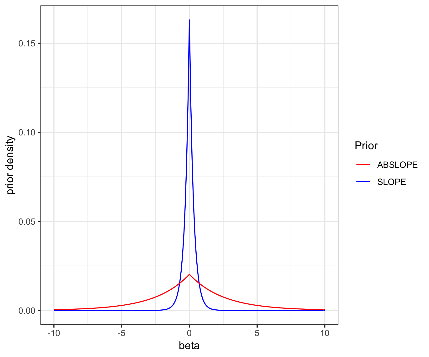
(a) Non-null $\beta$

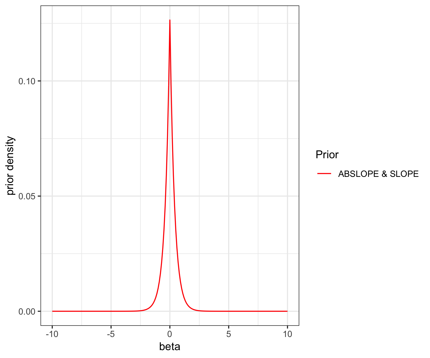
(b) Null $\beta$

Figure 1: Prior distribution of SLOPE and ABSLOPE, on $\beta$ whose true value is non-null (a) or null (b).

Figure 1 shows the difference between the SLOPE prior and the ABLSOPE prior on a single coefficient $\beta_{j}$. On the left, we have a slab prior distribution on an active coefficient $\beta_{j}$ which shows that ABSLOPE promotes larger estimates: the mass is greater in the tails compared to SLOPE. On the other hand, for the irrelevant $\beta_{j}$ (spike prior depicted on the right), ABSLOPE reduces to the double exponential SLOPE peak to threshold out small effects.

The ABSLOPE prior can be seen as a spike-and-slab prior, where the spike component models regression coefficients close to the noise level and the slab component models large regression coefficients. In fact, the spike-and-slab LASSO prior can be regarded as a special case when one considers the constant sequence of tuning parameters $\lambda_{1}=\ldots=\lambda_{p}=\lambda_{0}$ for the spike SLOPE component and $c$ as the ratio between spike and slab penalties. The algorithm described in Section 3.4 shows that the slab component is destined to de-bias the large regression coefficients while the spike component is aimed at FDR control.

2.4 Assumptions for missing values

We suppose that the missingness occurs only in the covariates $X$, not in the responses $y$. For each individual $i$, we denote with $X_{i,{\mathrm{o}bs}}$ the observed elements of $X_{i}=(X_{i1},X_{i2},\cdots,X_{ip})$ and with $X_{i,{\mathrm{m}is}}$ the missing ones. We also decompose the matrix of covariates as $X=(X_{{\mathrm{o}bs}},X_{{\mathrm{m}is}})$, keeping in mind that the missing elements may differ from one individual to another. For each individual $i$, we define the missing data indicator vector $m_{i}=(m_{ij},1\leq j\leq p)$, with $m_{ij}=1$ if $X_{ij}$ is missing and $m_{ij}=0$ otherwise. The matrix $m=(m_{i},1\leq i\leq n)$ then defines the missing data pattern. The missing data mechanism is characterized by the conditional distribution of $m$ given $X$ and $y$, with a parameter $\phi$, i.e., $\texttt{p}(m_{i}\mid X_{i},y_{i},\phi).$ In the literature on missing data (Little and Rubin, , 2002), three mechanisms (Rubin, , 1976) are recognized to describe the distribution/sources of missingness: i) Missing completely at random (MCAR): the absence is not related to any variable in the study; ii) Missing at random (MAR): the missing data depends only on the observed variables; iii) Missing not at random (MNAR): the absence depends on the value itself. Throughout this paper, we assume the MAR mechanism which implies that the missing values mechanism can therefore be ignored when maximizing the likelihood (Little and Rubin, , 2002). A reminder of these concepts is given in the Appendix A.2.

We adopt a probabilistic framework by assuming that $X_{i}=(X_{i1},\ldots,X_{ip})$ is normally distributed:

$$X_{i}\mathop{\sim}_{i.i.d.}\mathcal{N}_{p}(\mu,\Sigma),\quad i=1,\cdots,n\;.$$

Since the covariates should be standardized (as we assumed at the beginning of Section 2), we have to reconsider our scaling of $X$ in the light of missing data. When the missing values are MCAR, scaling can be performed as a pre-processing step before performing the analysis. Since observed values represent a random sample from the population, standard deviations estimated using observed data are unbiased estimates of the population standard deviation even if their variance is larger. When the missing data are MAR, standard deviations estimated using observed data can be severely biased. Indeed, consider the case when two variables are highly correlated and missing values occur in one variable when the values of the other variable are larger than a constant, then the estimated standard deviation will be biased downwards. Consequently, its estimation needs to be included in the analysis. In the Appendix A.3, we detail how we update mean and standard deviation at each iteration of the algorithm presented in Section 3.

2.5 Overview of modeling

Figure 2 shows our ABSLOPE graphical model with variables, parameters and their relations. We aim at estimating $\beta$ and $\sigma^{2}$, treating parameters $\mu$ and $\Sigma$ as nuisance.

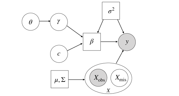
Figure 2: ABSLOPE graphical model. Arrows indicate dependencies. White circles are for latent variables, gray ones for observed variables and squares for parameters.

3 Parameter estimation and model selection

In this section, we develop an ABSLOPE method based on the stochastic approximation EM algorithm. As this algorithm entails proper sampling which can be quite time consuming, we also provide a simplified heuristic version called SLOBE, where the stochastic step is replaced with deterministic approximations of parameter expected values. This faster variant allows us to consider models of larger dimensions and, according to our simulation study, performs very similarly to the stochastic version.

3.1 Maximizing the observed penalized likelihood

According to the model defined in Section 2 and presented in Figure 2, the penalized complete-data log-likelihood can be written as:

$$\begin{split}\ell_{\mathrm{c}omp}=&\log\texttt{p}(y,X,\gamma,c;\,\beta,\theta,\sigma^{2})+pen(\beta)\\ =&\log\left\{\texttt{p}(X\mid\mu,\Sigma)\,\texttt{p}(y\mid X;\,\beta,\sigma^{2})\,\texttt{p}(\gamma\mid\theta)\,\texttt{p}(c)\right\}+pen(\beta)\\ =&-\frac{1}{2}\log(2\pi\lvert\Sigma\rvert)-\frac{1}{2}(X-\mu)^{T}\Sigma^{-1}(X-\mu)-n\log(\sigma)-\frac{1}{2\sigma^{2}}\|y-X\beta\|^{2}\\ &+\sum_{j=1}^{p}\mathbb{1}(\gamma_{j}=1)\log\theta+\sum_{j=1}^{p}\mathbb{1}(\gamma_{j}=0)\log(1-\theta)-\frac{1}{\sigma}\sum_{j=1}^{p}w_{j}\lvert\beta_{j}\rvert{\lambda_{r(W\beta,j)}}.\end{split}$$ (4)

Similarly as the EMVS variable selection procedure of Ročková and George, (2014), we focus on obtaining the MAP point estimates and do not aspire at fully Bayesian inference which would entail calculating the entire posterior distribution. Due to the presence of latent variables $X_{{\mathrm{m}is}},\gamma$ and $c$, we estimate $\beta$ by maximizing the observed log-likelihood which integrates over the latent variables: ${\ell}_{\mathrm{o}bs}=\iiint{\ell}_{\mathrm{c}omp}\,dX_{{\mathrm{m}is}}\,dc\,d\gamma.$ We use the EM algorithm (Dempster et al., , 1977) to estimate $\beta$, and in the meantime, obtain simulated $\gamma$ to distinguish the true signals from the noise, i.e. to select variables. Given the initialization, each iteration $t$ updates $\beta^{t}$ to $\beta^{t+1}$ with the following two steps:

• E step: The expectation of the complete-data log likelihood with respect to the conditional distribution of latent variables is computed, i.e.,

  $$Q^{t}=\mathbb{E}({\ell}_{\mathrm{c}omp})\quad\text{wrt}\quad\texttt{p}(X_{{\mathrm{m}is}},\gamma,c,\theta\mid y,X_{{\mathrm{o}bs}},\beta^{t},\sigma^{t},\mu^{t},\Sigma^{t})\;.$$

  Since this is not tractable, we derive a stochastic approximation EM (SAEM) algorithm (Lavielle, , 2014) by replacing the E step by a simulation step and a stochastic approximation step.

  • Simulation: draw one sample $(X_{{\mathrm{m}is}}^{t},\gamma^{t},c^{t},\theta^{t})$ from

    $$\texttt{p}(X_{{\mathrm{m}is}},\gamma,c,\theta\mid y,X_{{\mathrm{o}bs}},\beta^{t-1},\sigma^{t-1},\mu^{t-1},\Sigma^{t-1})\;;$$ (5)

  • Stochastic approximation: update function Q with

    $$Q^{t}=Q^{t-1}+\eta_{t}\left({\ell}_{\mathrm{c}omp}{\Big{|}}_{X_{{\mathrm{m}is}}^{t},\gamma^{t},c^{t},\theta^{t}}-Q^{t-1}\right)\;,$$ (6)

    where $\eta_{t}$ is the step-size.

  The step-size $(\eta_{t})$ is chosen as a decreasing sequence as described in Delyon et al., (1999) which ensures almost sure convergence of SAEM to a maximum of the observed likelihood in their continuously differentiable case.

• M step: $(\beta^{t+1},\sigma^{t+1},\mu^{t+1},\Sigma^{t+1})=\operatorname*{arg\,max}Q^{t+1}.$
  Note that $\Sigma^{t+1}$ is estimated as above only when $p<<n$. Otherwise we consider a shrinkage estimation as discussed in Remark 1. Indeed, we regard $(\mu,\Sigma)$ as auxiliary parameters, which are needed only to update the missing values.

Despite the apparent complexity of the algorithm, it turns out that the likelihood (4) can be decomposed into several terms: one term for the linear regression part, one term for the covariates distribution and terms for the latent variables $\gamma$ and $c$, as illustrated in Figure 2. Consequently, one iteration can be divided into tractable sub-problems, as detailed in the following subsections.

3.2 Simulation step: sampling the latent variables

To perform the simulation step (5), we use the Gibbs sampler. To simplify notation, we hide the superscript and note that all conditional distributions are computed given the quantities from the previous iteration. We perform the following sampling procedure:

$$\begin{cases}\,\gamma\sim Bin\left(\frac{\theta c\exp\left(-c{\frac{1}{\sigma}}\lvert\beta_{j}\rvert\lambda_{r(W\beta,j)}\right)}{(1-\theta)\exp\left(-{\frac{1}{\sigma}}\lvert\beta_{j}\rvert\lambda_{r(W\beta,j)}\right)+\theta c\exp\left(-c{\frac{1}{\sigma}}\lvert\beta_{j}\rvert\lambda_{r(W\beta,j)}\right)}\right)\,;\\ \,\theta\sim Beta\left(a+\sum_{j=1}^{p}\mathbb{1}(\gamma_{j}=1),b+\sum_{j=1}^{p}\mathbb{1}(\gamma_{j}=0)\right),\text{ with }Beta(a,b)\text{ a prior for }\theta\,;\\ \,c\sim Gamma\left(1+\sum_{j=1}^{p}\mathbb{1}(\gamma_{j}=1),\quad\frac{1}{\sigma}\sum_{j=1}^{p}\lvert\beta_{j}\rvert\lambda_{r(W\beta,j)}\mathbb{1}(\gamma_{j}=1)\right)\text{ truncated to }[0,1].\end{cases}$$ (7)

The detailed calculation and interpretation can be found in Appendix A.4. In addition, to simulate the missing values $X_{{\mathrm{m}is}}$, we perform a decomposition:

$$\begin{split}X_{{\mathrm{m}is}}&\sim\texttt{p}(X_{{\mathrm{m}is}}\mid\gamma,c,y,X_{{\mathrm{o}bs}},\beta,\sigma,\theta,\mu,\Sigma)\\ &=\texttt{p}(X_{{\mathrm{m}is}}\mid y,X_{{\mathrm{o}bs}},\beta,\sigma,\mu,\Sigma)\\ &\propto\texttt{p}(y\mid X_{{\mathrm{o}bs}},X_{{\mathrm{m}is}},\beta,\sigma)\,\texttt{p}(X_{{\mathrm{m}is}}\mid X_{{\mathrm{o}bs}},\mu,\Sigma)\;.\end{split}$$ (8)

Here, we observe that the target distribution (8) is a normal distribution since the two terms after factorization are both normal. In the following proposition, we give the explicit form of the target distribution as a solution to a system of linear equations.

Proposition 1.

For a single observation $x=(x_{{\mathrm{m}is}},x_{{\mathrm{o}bs}})$ we denote with $x_{{\mathrm{o}bs}}$ and $x_{{\mathrm{m}is}}$ observed and missing covariates, respectively. Let $\mathcal{M}$ be the set containing indexes for missing covariates and $\mathcal{O}$ for the observed ones. Assume that $p(x_{{\mathrm{o}bs}},x_{{\mathrm{m}is}};\Sigma,\mu)\sim\mathcal{N}(\mu,\Sigma)$ and let $y=x\beta+\varepsilon$ where $\varepsilon\sim N(0,\sigma^{2})$. For all the indexes of the missing covariates $i\in\mathcal{M}$, we denote:

$$m_{i}=\sum_{q=1}^{p}\mu_{j}s_{iq},\quad u_{i}=\sum_{k\in\mathcal{O}}x_{{\mathrm{o}bs}}^{k}s_{ik},\quad r=y-x_{{\mathrm{o}bs}}{\beta_{\mathrm{o}bs}},\quad\tau_{i}=\sqrt{s_{ii}+\beta_{i}^{2}/\sigma^{2}}\;,$$

with $s_{ij}$ elements of $\Sigma^{-1}$ and ${\beta_{\mathrm{o}bs}}$ the observed elements of $\beta$.
Let $\tilde{\mu}=(\tilde{\mu}_{i})_{i\in\mathcal{M}}$ be the solution of the following system of linear equations:

$$\frac{r\beta_{i}/\sigma^{2}+m_{i}-u_{i}}{\tau_{i}}-\sum_{j\in\mathcal{M},j\neq i}\frac{\beta_{i}\beta_{j}/\sigma^{2}+s_{ij}}{\tau_{i}\tau_{j}}\tilde{\mu}_{j}=\tilde{\mu}_{i}\;,\quad\text{for all }i\in\mathcal{M}\;,$$ (9)

and let $B$ be a matrix with elements:

$$B_{ij}=\begin{cases}\frac{\beta_{i}\beta_{j}/\sigma^{2}+s_{ij}}{\tau_{i}\tau_{j}},&\text{if }i\neq j\\ 1,&\text{if }i=j\end{cases}\;,$$

then for $z=(z_{i})_{i\in\mathcal{M}}$ where $z_{i}=\tau_{i}x_{{\mathrm{m}is}}^{i}$ we have:

$$z\mid x_{{\mathrm{o}bs}},y;\Sigma,\mu,\beta,\sigma^{2}\sim N(\tilde{\mu},B^{-1})\;.$$

As a result, we can simulate missing covariates from:

$$x_{{\mathrm{m}is}}\mid x_{{\mathrm{o}bs}},y;\Sigma,\mu,\beta,\sigma^{2}\sim N(\tilde{\mu}\oslash\tau,B^{-1}\oslash(\tau\tau^{T}))\;,$$

where $\tau=(\tau_{i})_{i\in\mathcal{M}}$ $\oslash$ is used for Hadamard division. The proof is provided in Appendix A.5.

3.3 Stochastic approximation and maximization steps

After the simulation step, we obtain one sample for each latent variable: $X_{{\mathrm{m}is}}^{t},\gamma^{t}$, $c^{t}$, and thus $W^{t}$ with diagonal elements $w^{t}_{j}=1-(1-c^{t})\gamma_{j}^{t}$. Now we have several parameters to estimate, but each parameter only concerns some of the terms in the complete-data likelihood. This helps us simplify calculations. The maximization step is nevertheless quite difficult because the complete model does not belong to a regular exponential family (if so we could update the sufficient statistics and maximize more easily).

As the implementation of SAEM is quite challenging in the general step-size case, we start with the simpler case of fixed step-size $\eta_{t}=1$. It is important to note that this causes larger variance compared to setting the step-size as a decreasing sequence (Delyon et al., , 1999) and there is no guarantee of convergence to the actual mode, only to its neighborhood.

3.3.1 Step-size $\eta_{t}=1$

When $\eta_{t}=1$, estimation boils down to maximizing the complete-data likelihood completed by sampling the latent variables from their conditional distribution given the observed values .

1. Update $\beta$.

   $$\begin{split}\beta^{t}=\operatorname*{arg\,max}_{\beta}Q_{1}^{t}(\beta):=-\frac{1}{2{(\sigma^{t-1})}^{2}}\|y-X^{t}\beta\|^{2}-\frac{1}{\sigma^{t-1}}\sum_{j=1}^{p}w^{t}_{j}\lvert{\beta_{j}}\rvert{\lambda_{r(W^{t}\beta,j)}}\,,\end{split}$$

   where $X^{t}=(X_{{\mathrm{o}bs}},X_{{\mathrm{m}is}}^{t})$. This estimate corresponds to the solution of SLOPE, given the value of $W$, $X_{{\mathrm{m}is}}$ and $\sigma$. In our implementation of ABSLOPE we solve the SLOPE optimization problem using the Alternative Direction Method of Multipliers of (Boyd et al., , 2011), which turns out to be much quicker then the proximal gradient algorithm of (Bogdan et al., , 2015) when the regressors are strongly correlated or when they are on different scales, as in our reweighting scheme.

2. Update $\sigma$.

   $$\begin{split}\sigma^{t}=\operatorname*{arg\,max}_{\sigma}Q_{2}^{t}(\sigma):=-n\log(\sigma)-\frac{1}{2\sigma^{2}}\lVert y-X^{t}\beta^{t}\rVert^{2}-\frac{1}{\sigma}\sum_{j=1}^{p}w^{t}_{j}\lvert\beta^{t}_{j}\rvert{\lambda_{r(W^{t}\beta^{t},j)}}\;.\end{split}$$

   Given by the derivative, the solution to estimate $\sigma$ is:

   $$\sigma^{t}=\frac{1}{2n}\left[\sum_{j=1}^{p}\lambda_{r(W^{t}\beta^{t},j)}w^{t}_{j}\lvert\beta^{t}_{j}\rvert+\sqrt{\left(\sum_{j=1}^{p}\lambda_{r(W^{t}\beta^{t},j)}w^{t}_{j}\lvert\beta^{t}_{j}\rvert\right)^{2}+4n\mathrm{RSS}}\right]\;,$$ (10)

   where the RSS (residual sum of squares) is $\lVert y-X^{t}\beta^{t}\rVert^{2}$.

   If we omit the penalization term, (10) amounts to $\sigma^{t}=\sqrt{\frac{RSS}{n}}$, which is the classical formula for MLE of $\sigma$ when $\beta$ is also estimated by MLE. In this case this estimator would be biased downwards. Interestingly, our posterior mode estimator of $\sqrt{n}\sigma$ is larger than the corresponding RSS, which, according to the simulation results in Subsection 4.2, often leads to a less biased estimator when most of the true effects are detected by ABSLOPE.

3. Update $\mu,\Sigma$:

   $$\mu^{t},\Sigma^{t}=\operatorname*{arg\,max}_{\mu,\Sigma}-\frac{1}{2}\log(2\pi\lvert\Sigma\rvert)-\frac{1}{2}(X^{t}-\mu)^{\top}\Sigma^{-1}(X^{t}-\mu)\;.$$

   When $p<<n$, the solution is given by the empirical mean and the empirical covariance matrix:

   $$\begin{split}\mu^{t}=\bar{X}^{t}=\frac{1}{n}\sum_{i=1}^{n}X_{i}^{t}\quad\text{and}\quad\Sigma^{t}=\frac{1}{n}\sum_{i=1}^{n}(X_{i}^{t}-\bar{X}^{t})(X_{i}^{t}-\bar{X}^{t})^{\top}\;.\end{split}$$

   In high dimensional setting, estimation of $\Sigma^{t}$ by the empirical covariance matrix is replaced by shrinkage estimation, as discussed in Remark 1.

Remark 1.

To tackle the problem of estimation and inversion of the covariance matrix in high dimensions, one can resort to shrinkage estimation as detailed in Ledoit and Wolf, (2004). With the assumption that the ratio $\frac{n}{p}$ is bounded, they propose an optimal linear shrinkage estimator as a linear combination of identity matrix $I_{p}$ and the empirical covariance matrix $S$, i.e.:

$$\hat{\Sigma}=\rho_{1}I_{p}+\rho_{2}S,\qquad\text{where }\rho_{1},\rho_{2}=\operatorname*{arg\,min}_{\rho_{1},\rho_{2}}\mathbb{E}\|\hat{\Sigma}-\Sigma\|^{2}\;.$$

The method boils down to shrinking empirical eigenvalues towards their mean. The parameters $\rho_{1}$ and $\rho_{2}$ are chosen with asymptotically (as $n$ and $p$ go to infinity) uniformly minimum quadratic risk in its class.

3.3.2 General step-size

With a general step-size (say $\eta_{t}=\frac{1}{t}$), for a model parameter $\psi$ we set

$$\psi^{t+1}=\psi^{t}+\eta_{t}\left[\hat{\psi}^{t}_{MLE}-\psi^{t}\right]\;,$$ (11)

where $\hat{\psi}^{t}_{MLE}$ is the MLE estimator of the complete-data likelihood completed by drawing the latent variables from their conditional distributions given the observed information. This exactly corresponds to the estimate in Subsection 3.3.1 when $\eta_{t}=1$. In other words, we apply stochastic approximations on the model parameters, instead of directly operating on the likelihood in (6). When the likelihood (4) is a linear function of the parameters, the stochastic approximation step in equation (6) corresponds exactly to our proposal (11). In other situations, it gives good results from an empirical point of view.

3.4 SLOBE: Quick version of ABSLOPE

The implementation of SAEM, as described in Subsection 3.2 and 3.3, can still be costly in terms of computation time, even if the terms of the likelihood decompose well and we use the approximation (11). We therefore propose a simplified version of the algorithm, called SLOBE, which instead of drawing samples $(X_{{\mathrm{m}is}}^{t},\gamma^{t},c^{t},\theta^{t})$ from their conditional distribution (5) in the simulation step, approximates them by their conditional expectation, i.e.,

$$(X_{{\mathrm{m}is}}^{t},\gamma^{t},c^{t},\theta^{t})\leftarrow\mathbb{E}(X_{{\mathrm{m}is}},\gamma,c\mid y,X_{{\mathrm{o}bs}},\beta^{t-1},\sigma^{t-1},\mu^{t-1},\Sigma^{t-1})\;;$$

To simplify notation, we hide the superscript, but note that all the conditional expectations are computed given the quantities from the previous iteration.

1. Approximate $\gamma_{j}$ by:

   $$\begin{split}\pi&\coloneqq\mathbb{E}(\gamma_{j}=1\mid\gamma_{-j},c,\beta,\sigma,\theta,W)=p(\gamma_{j}=1\mid\gamma_{-j},c,\beta,\sigma,\theta,W)\\ &\stackrel{{\scriptstyle\text{(\ref{eq:simu})}}}{{=}}\frac{\theta c\exp\left(-c{\frac{1}{\sigma}}\lvert\beta_{j}\rvert\lambda_{r(W\beta,j)}\right)}{(1-\theta)\exp\left(-{\frac{1}{\sigma}}\lvert\beta_{j}\rvert\lambda_{r(W\beta,j)}\right)+\theta c\exp\left(-c{\frac{1}{\sigma}}\lvert\beta_{j}\rvert\lambda_{r(W\beta,j)}\right)}\;.\end{split}$$ (12)

2. Approximate $\theta$ by:

   $$\begin{split}\mathbb{E}(\theta\mid\gamma,y,X_{{\mathrm{o}bs}},X_{{\mathrm{m}is}},\beta,\sigma,c,\mu,\Sigma,W)=\mathbb{E}(\theta\mid\gamma,\beta,\sigma,W)\stackrel{{\scriptstyle\text{(\ref{eq:simu})}}}{{=}}\frac{a+\sum_{j=1}^{p}\mathbb{1}(\gamma_{j}=1)}{a+b+p}\;,\end{split}$$ (13)

   where $a$ and $b$ are fixed parameters in the prior of $\theta$.

3. Approximate $c$ by:

   $$\begin{split}\mathbb{E}(c\mid\gamma,y,X_{{\mathrm{o}bs}},X_{{\mathrm{m}is}},\beta,\sigma,\theta,\mu,\Sigma,W)\stackrel{{\scriptstyle\text{(\ref{eq:c})}}}{{=}}\frac{\int_{0}^{1}x^{a^{\prime}}\exp(-b^{\prime}x)dx}{\int_{0}^{1}x^{a^{\prime}-1}\exp(-b^{\prime}x)dx}\;,\end{split}$$ (14)

   where $a^{\prime}=1+\sum_{j=1}^{p}\mathbb{1}(\gamma_{j}=1)$, $b^{\prime}=\frac{1}{\sigma}\sum_{j=1}^{p}\lvert\beta_{j}\rvert\lambda_{r(W\beta,j)}\mathbb{1}(\gamma_{j}=1)$.

4. In the case with missing values, for the $i^{\mathrm{t}h}$ observation $X_{i}$, approximate $X_{i,{\mathrm{m}is}}$ by:

   $$\mathbb{E}(X_{i,{\mathrm{m}is}}\mid\gamma,c,y,X_{i,{\mathrm{o}bs}},\beta,\sigma,\theta,\mu,\Sigma)=\mathbb{E}(X_{i,{\mathrm{m}is}}\mid y,X_{i,{\mathrm{o}bs}},\beta,\sigma,\mu,\Sigma)\;,$$

   which is provided by Proposition 1.

Then, in step M, we maximize the likelihood of the complete data, as in Subsection 3.3.1. The impact of replacing the simulation step with a conditional expectation is that we ignore the variability of latent variable sampling, which in high dimensional settings helps reduce noise of the algorithm, and which also leads to accelerations as shown in our simulation study in Subsection 4.5. We provide a summary of ABSLOPE and SLOBE methods in Appendix A.6.

4 Simulation study

4.1 Simulation setting

To illustrate the performance of our methodology, we perform simulations by first generating data sets as follows:

1. A design matrix $X_{n\times p}$ is generated from a multivariate normal distribution $\mathcal{N}(\mu,\Sigma)\;$. The matrix is standardized, s.t., the mean of each column is 0 and its $\ell_{2}$-norm is 1.

2. The signal magnitude is $c_{0}\sqrt{2\log p}$ when $c_{0}$ is large the signal strength is stronger. Only $k$ on the $p$ predictors are non-zero and all equal to $c_{0}\sqrt{2\log p}$.

3. The response vector is generated from $y=X\beta+\epsilon$ with $\epsilon\sim N(0,\sigma^{2}I_{n})$ and $\sigma=1$ to start.

4. Missing values are entered into the design matrix using a MCAR or MAR mechanism. For the former, we randomly generate 10% of missing cells; for the later, we follow the multivariate imputation procedure proposed by Schouten et al., (2018).

We set the initialization and the hyperparameters as follows.

Initialization

Appendix A.7 provides the default values we have taken for the following simulation studies. The algorithm is not sensitive to the choice of values $a$ and $b$ (12), but initial values for $\beta$ may have a stronger impact. In practice, we use the LASSO estimates based on preliminary mean imputation (missing values replaced by the average of the observed values for each variable) to initialize the coefficients.

Step-size

We set $\eta_{t}=1$ for the first $t_{0}=20$ iterations to approach the neighborhood of the MLE, then, choose a positive decreasing sequence $\eta_{t}=\frac{1}{t-t_{0}}$ to approximate the MLE, with the stochastic approach formula (11).

$\lambda$ sequence

A sequence of penalty coefficients $\lambda$ must be chosen before implementing the algorithm. As introduced in the Subsection 2.1, we use a BH sequence inspired by orthogonal designs:

$$\lambda_{BH}(j)=\phi^{-1}(1-q_{j}),\quad q_{j}=\frac{jq}{2p},\quad j=1,2,\cdots,p.$$

4.2 Convergence of SAEM

We first illustrate the convergence of SAEM. We set the size of design matrix as $n=p=100$ while the number of true predictors is $k=10$, the signal strength $3\sqrt{2\log p}$ and the percentage of missingness $10\%$. The covariance $\Sigma$ is an identity matrix to start.

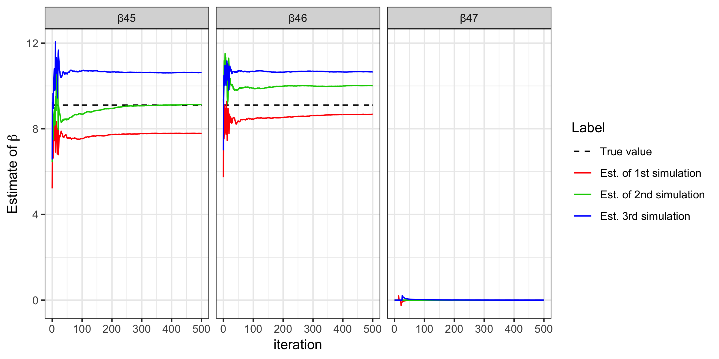
Figure 3: Convergence plots for three coefficients with ABSLOPE (colored solid curves). Black dash lines represent the true value for each $\beta$. Estimates obtained with three different sets of simulated data are represented by three different colors.

Figure 3 shows the convergence of some coefficients with SAEM for three simulated data sets. These graphs are representative of all the observed results. There are large fluctuations during the first $t_{0}=$20 iterations, then after introducing the stochastic approximation at the 20th iteration, convergence is achieved gradually. Due to the existence of a sorted $l_{1}$ penalty, the estimates are still slightly biased.

In addition, we also represent the convergence curves for $\sigma$ with ABSLOPE in supplementary materials (Jiang et al., 2019a, ) in order to compare the estimate of $\sigma$ by ABSLOPE to the biased MLE estimator without prior knowledge, i.e., $\hat{\sigma}_{\mathrm{M}LE}=\sqrt{\frac{RSS}{n}}$. We can see that the estimates of $\sigma$ with both methods are biased downward, but since ABSLOPE has an additional correction term (10), it leads to a less biased estimator.

4.3 Behavior of ABSLOPE - SLOBE

We then evaluate ABSLOPE and SLOBE in a different parametrization setting to see how the signal strength, sparsity and other parameters influence their performance.

Criterion

We apply ABSLOPE or SLOBE on a synthetic dataset and get estimates for $\hat{\beta}$ and the sampled $\hat{\gamma}$ indicating the model selection results. We compare the selected model to the true one. The total number of true discoveries is $TP=\#\{j:|\beta_{j}\rvert>0\text{ and }|\hat{\beta}_{j}\rvert>0\}$ and the total number of false discoveries is $FN=\#\{j:|\beta_{j}\rvert>0\text{ and }\hat{\beta}_{j}=0\}$.

To evaluate the performance, we consider the following quantities:

• Power $=\frac{TP}{TP+FN}$;

• FDR $=\frac{FP}{FP+TP}$ ;

• MSE of $\beta$ (Relative $l_{2}$ norm error) $=\frac{\|\hat{\beta}-\beta\rVert^{2}}{\|\beta\rVert^{2}}$;

• Relative prediction error $=\frac{\|X\hat{\beta}-X\beta\rVert^{2}}{\|X\beta\rVert^{2}}$.

For each set of parameters, we repeat the procedure 200 times: i) data generation ii) estimation and model selection with ABSLOPE/SLOBE iii) evaluation with the criteria presented above and we compute the means over the 200 simulations. The simulations were implemented with parallel computing.

4.3.1 Scenario 1

We first consider $n=p=100$ and vary:

• sparsity: number of true signal $k=5,\,10,\,15,\,20$;

• signal strength $\sqrt{2\log p}\,,2\sqrt{2\log p}\,,3\sqrt{2\log p}\,,4\sqrt{2\log p}$;

• percentage of missingness $0.1,\,0.2,\,0.3$, generated randomly, i.e., MCAR;

• correlation between covariates $\Sigma=\text{toeplitz}(\rho)$ where $\rho=0,\,0.5,\,0.9$.

Then we applied the Algorithm 1 on each synthetic dataset.

Results 1: no correlation, 10% missingness - vary signal strength

According to Figure 4:

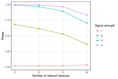
(a) Power

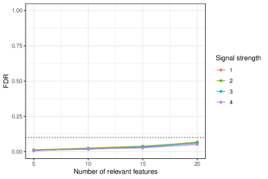
(b) FDR

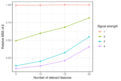
(c) Bias of $\beta$

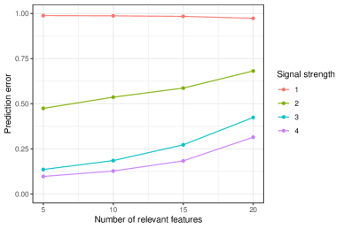
(d) Prediction error

Figure 4: Mean of power (a), FDR (b), bias of the estimate for $\beta$ (c) and prediction error (d), as function of length of true signal, over the 200 simulations. Results for $n=p=100$, percentage of missingness $10\%$ and $\Sigma$ orthogonal (no correlation).

• We observe that FDR is always controlled at the expected level 0.1.

• Power increases and estimation bias decreases with larger sparsity or stronger signal.

• When the signal is too weak (signal strength = $\sqrt{2\log p}$), the power is near 0, which is due to the identifiablility issue that ABSLOPE cannot distinguish the signal from the noise. Indeed, the value $c=\frac{\lambda_{1}}{\sigma\sqrt{2\log p}}$ is greater than one where $\lambda_{1}$ is the largest penalization coefficient. In addition, the bias is significant. This behaviour can be explained by the fact that we choose the penalty $\lambda$ to reduce the noise $\sigma$; but when the signal is as weak as $\sigma$, this choice of $\lambda$ also ”kills” the real signal.

Results 2: with correlation, strong signal - vary percentage of missingness

Now we add the correlation as $\Sigma=\text{toeplitz}(\rho)$ where $\rho=0.5$, and also fix a strong signal strength as $3\sqrt{2\log p}$. We then vary the sparsity and percentage of missingness. The results in Figure 5 show that:

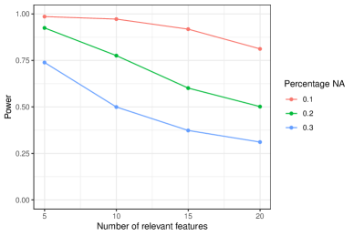
(a) Power

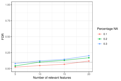
(b) FDR

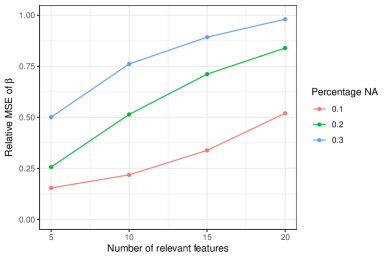
(c) Bias of $\beta$

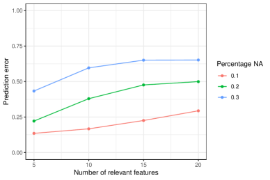
(d) Prediction error

Figure 5: Mean of power (a), FDR (b), bias of the estimate for $\beta$ (c) and prediction error (d), as function of length of true signal over the 200 simulations. Results for $n=p=100$, with correlation and strong signal.

• The power increases and the estimation bias decreases when the percentage of missing data decreases.

• In the presence of correlation, the FDR control is slightly lost when the number of non-zero coefficients is greater than 10 and the percentage of missing values exceeds 0.2, but is still near the nominal level.

4.3.2 Scenario 2

Now we consider a larger dataset $n=p=500$ and vary the same parametrization as in Subsection 4.3.1, except the sparsity, for which we take wider range of choices among $k=10,\,20,\,30,\,\cdots,\,60$. In this scenario of larger dimension, we have applied the simplified SLOBE algorithm as described in Subsection 3.4 to avoid intensive computation.

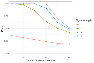
(a) Power

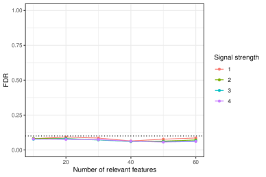
(b) FDR

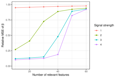
(c) Bias of $\beta$

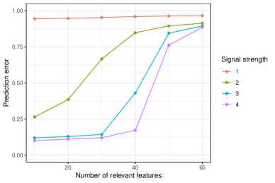
(d) Prediction error

Figure 6: Mean of power (a), FDR (b), bias of the estimate for $\beta$ (c) and prediction error (d), as function of length of true signal, over the 200 simulations. Results for $n=p=500$, percentage of missingness $10\%$ and $\Sigma$ orthogonal (no correlation).

Results 1: no correlation, 10% missingness - vary signal strength

According to Figure 6:

• FDR is always controlled at expected level 0.1.

• Similar to Figure 4, power increases and estimation error decreases with larger sparsity and stronger signal. However in this larger dimension case, we can handle with larger number of relevant features until 30 or 40, at which we observe a phase transition due to the identifiability issue.

Results 2: with correlation, strong signal - vary percentage of missingness

Now we add the correlation as $\Sigma=\text{toeplitz}(\rho)$ where $\rho=0.5$, and also fix a strong signal strength as $3\sqrt{2\log p}$. We then vary the sparsity and percentage of missingness. The results in Figure 7 show that:

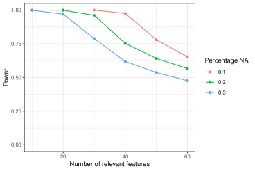
(a) Power

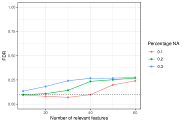
(b) FDR

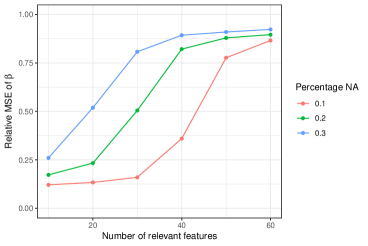
(c) Bias of $\beta$

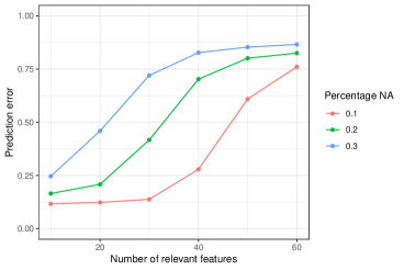
(d) Prediction error

Figure 7: Mean of power (a), FDR (b), bias of the estimate for $\beta$ (c) and prediction error (d), as function of length of true signal over the 200 simulations. Results for $n=p=500$, with correlation and strong signal.

• Similar to Figure 5, the power increases and the estimation error decreases when the percentage of missing data decreases.

• Due to the existence of correlation, the FDR control is slight lost, especially in the less sparse and more missing case.

• With 10% missing values, if the number of relevant features is below 40, then we can always achieve an efficient power and perfect FDR control. With larger percentage of missing values, the sparsity of this changing point will be more conservative.

In addition, we present the results varying the correlations in the supplementary materials (Jiang et al., 2019a, ).

4.4 Comparison with competitors

We use the same simulation scenario and criteria as those used in Subsection 4.3 to compare ABSLOPE and SLOBE to other approaches that can be considered to select variables in the presence of missing data.

• ncLASSO: Non-convex LASSO (Loh and Wainwright, , 2012)

• Methods based on preliminary mean imputation (MeanImp): missing values are replaced by the average of the observed values for each variable, then on the completed data set is applied:

  • SLOPE: Applying two steps i) SLOPE (Bogdan et al., , 2015) ii) OLS on the selected predictors to estimate the parameters;

  • LASSO: LASSO with $\lambda$ selected by cross validation;

  • adaLASSO: adaptive LASSO (Zou, , 2006);

For SLOPE, ABSLOPE and SLOBE, we set the penalization coefficient $\lambda$ as the BH sequence which controls the FDR at level $0.1$. The values of the tuning parameters for the different methods can be found in the available code on GitHub (Jiang, , 2019). We try to make the comparisons as fair as possible and also favor the competitors: we give the true $\sigma$ to SLOPE whereas we estimate it with ABSLOPE. ncLASSO requires to specify a bound on the $l_{1}$ norm of the coefficients, i.e., $\beta<R=b_{0}\#\{\beta_{j}:\beta_{j}\neq 0\}$, for which we take the real value of sparsity and signal strength.

Note that we do not make comparisons with the widely used multiple imputation (van Buuren and Groothuis-Oudshoorn, , 2011), where several imputed values are made for each missing value to reflect the uncertainty in the missingness. There are several reasons, including the inability to perform model selection with multiple imputation and the difficulty to aggregate the estimates from the imputed datasets.

We present the results for the case $n=p=100$ in the supplementary materials (Jiang et al., 2019a, ) while Figure 8 summarizes the result for the case $n=p=500$, 10% missingness and with correlation $\text{toeplitz}(0.5)$. Lighter colors indicate smaller values.

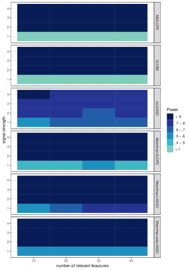
(a) Power

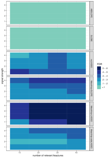
(b) FDR

(c) Bias of $\beta$

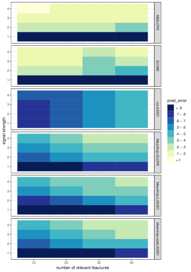
(d) Prediction error

Figure 8: Comparison of power (a), FDR (b), bias of $\beta$ (c) and prediction error (d) with varying sparsity and signal strength, with 10% missingness over 200 simulations in the case with correlation.

• ABSLOPE and SLOBE both have strong power and accurate prediction, where FDR is always controlled.

• The power and FDR control achieved by ABSLOPE and SLOBE are better than the case $n=p=100$. On one hand, correlation helps the generation of missing values. On the other hand, sparsity considered here is less complicated.

• Other methods pay the price of FDR control to achieve good power.

4.5 Comparison of computation time

Table 1 presents the execution time of the different methods considered in the simulation. In addition, we have implemented our proposed algorithm in C and we use Rcpp (Eddelbuettel and Balamuta, , 2017) to integrate these functions within R.

Table 1: Comparison of average execution time (in seconds) for one simulation, in the case without correlation and with $10\%$ MCAR, for $n=p=100$ and $n=p=500$ calculated over 200 simulations. (MacBook Pro, 2.5 GHz, processor Intel Core i7)

Execution time (seconds) $\boldsymbol{n=p=100}$ $\boldsymbol{n=p=500}$ for one simulation min mean max min mean max ABSLOPE 12.83 14.33 20.98 646.53 696.09 975.73 SLOBE 0.53 0.60 0.98 35.82 39.18 57.66 SLOBE (with Rcpp) 0.31 0.34 0.66 14.23 15.07 29.52 MeanImp + SLOPE 0.01 0.02 0.09 0.24 0.28 0.53 ncLASSO 16.38 20.89 51.35 91.90 100.71 171.00 MeanImp + LASSO 0.10 0.14 0.32 1.75 1.85 3.06 MeanImp + adaLASSO 0.45 0.58 1.12 45.06 47.20 71.24

In the case $n=p=100$, we observe that the most time consuming method is ncLASSO, which spent on average 20 seconds on one simulation. While ABSLOPE also took on average 14 seconds for one run, its simplified version SLOBE reduced this cost to 0.6 seconds, which is comparable to MeanImp + adaLASSO. While when $n=p=500$, the convergence of ABSLOPE requires much more time but SLOBE helps to simplify the complexity. In addition, the version of C for SLOBE is more accelerated, saving half of the computation time, which makes SLOBE capable of handling larger datasets.

5 Application to Traumabase dataset

5.1 Details on the dataset and preprocessing

Our work is motivated by an ongoing collaboration with the TraumaBase group at APHP (Public Assistance - Hospitals of Paris), which is dedicated to the management of severely traumatized patients. Major trauma is defined as any injury that endangers life or functional integrity of a person. The WHO has recently shown that major trauma in its various forms, including traffic accidents, interpersonal violence, self-harm, and falls, remains a public health challenge and a major source of mortality and handicap around the world (Hay et al., , 2017). Effective and timely management of trauma is critical to improving outcomes. Delays and/or errors in treatment have a direct impact on survival, especially for the two main causes of death in major trauma: hemorrhage and traumatic brain injury. Using patients’ records measured in the prehospital stage or on arrival to the hospital, we aim to establish prediction models in order to prepare an appropriate response upon arrival at the trauma center, e.g., massive transfusion protocol and/or immediate haemostatic procedures. Such models intend to give support to clinicians and professionals. Due to the highly stressful multi-player environment, evidence suggests that patient management – even in mature trauma systems – often exceeds acceptable time frames (Hamada et al., , 2014). In addition, discrepancies may be observed between diagnoses made by emergency doctors in the ambulance and those made when the patient arrives at the trauma center (Hamada et al., , 2015). These discrepancies can result in poor outcomes such as inadequate hemorrhage control or delayed transfusion.

To improve decision-making and patient care, six trauma centers within the Ile de France region (Paris area) in France have collaborated to collect detailed high-quality clinical data from accident scenes to the hospital. These centers have joined TraumaBase progressively between January 2011 and June 2015. The database integrates algorithms for consistency and coherence and data monitoring is performed by a central administrator. Sociodemographic, clinical, biological and therapeutic data (from the prehospital phase to the discharge) are systematically recorded for all trauma patients, and all patients transported in the trauma rooms of the participating centers are included in the registry. The resulting database now has data from 7495 trauma cases with more than 250 variables, collected from January 2011 to March 2016, with age ranged from 12 to 96, and is continually updated. The granularity of collected data makes this dataset unique in Europe. However, the data is highly heterogeneous, as it comes from multiple sources and, furthermore, is plagued with missing values, which makes modeling challenging.

In our analysis, we have focused on one specific challenge: developing a statistical model with missing covariates in order to predict the level of platelet upon arrival at the hospital. This model can aid creating an innovative response to the public health challenge of major trauma. The platelet is a cellular agent responsible for clot formation. It is essential to control its levels to prevent blood loss as quickly as possible in order to reduce early mortality in severely traumatized patients. It is difficult to obtain the level of platelet in real time on arrival at hospital and, if available, its levels would determine how the patients are treated. Accurate prediction of this metric is thereby crucial for making important treatment decisions in real time.

We focus on patients after an accident who were sent directly to the hospital (not sent to Emergency Care Unit). After this pre-selection, 6384 patients remained in the data set. Based on clinical experience, in order to predict the level of platelet on arrival at the hospital, 15 influential quantitative measurements were included as pre-selected variables. Detailed descriptions of these measurements are shown in the supplementary materials (Jiang et al., 2019a, ). These variables were included here because they were all available to the pre-hospital team, and therefore could be used in real situations.

Figure 9 shows the percentage of missingness per variable, varying from 0 to 60%. If we were to perform the complete case analysis (i.e., ignoring all the observations with missing values) only less than one third of the observations (1648 patients) would still remain in the dataset. This loss of data demonstrates the importance of appropriately handling the missing values.

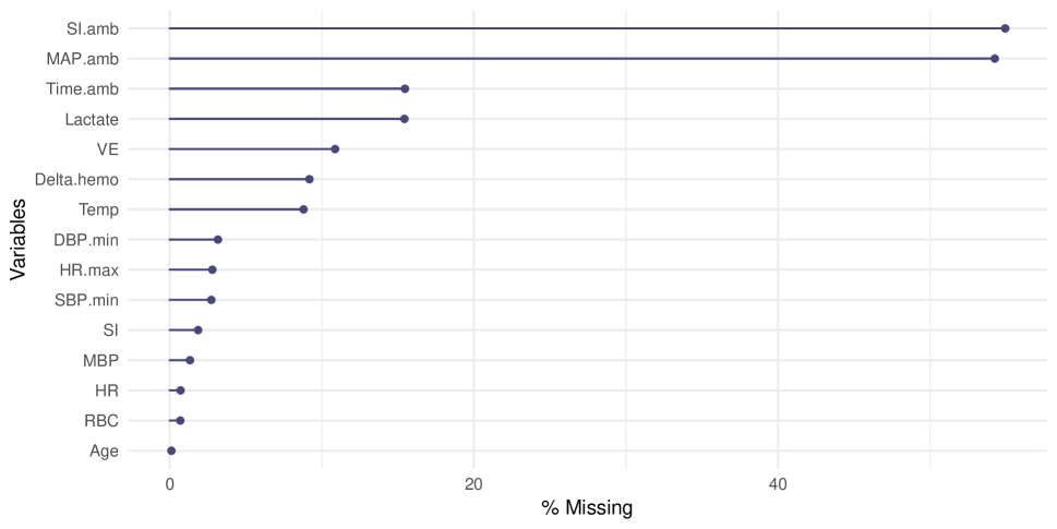
Figure 9: Percentage of missing values in each pre-selected variable from TraumaBase.

5.2 Model selection results

As is customary in supervised learning, we divide the dataset into training and test sets. The training set contains a random selection of 80% of observations whereas the test set contains the remaining 20%. In the training set, we select a model and estimate the parameters. We apply ABSLOPE and compare it with the same methods than those described in Section 4, namely MeanImp + SLOPE, MeanImp + LASSO, MeanImp + adaLASSO, MeanImp + SSL except ncLASSO since we do not known the sparsity and the $l_{1}$ bound of coefficients. Moreover, we also include:

• BIC: Mean imputation followed by a stepwise method based on BIC;

• RF: Mean imputation followed by a random forest (Liaw and Wiener, , 2002). This approach is assessed only for its prediction properties as it does not explicitly select variables.

In the SLOPE type methods, we set the penalization coefficient $\lambda$ as BH sequence which controls the FDR at level $0.1$. Since we consider our design matrix being centered and without an intercept, we also center the vector of responses and apply the procedure on $\tilde{y}=y-\bar{y}$, where $\bar{y}$ is the mean of $y$. We repeat the procedure of data splitting (into training and test sets) 10 times and Table 3 shows that, over 10 replications, how many times each variable is selected. In addition, Table 3 reports whether the selected variables by ABSLOPE have on average a positive or negative effect on the platelet.

Table 2: Number of times that each variable is selected over 10 replications. Bold numbers indicate which variables are included in the model selected by ABSLOPE.

Variable ABSLOPE SLOPE LASSO adaLASSO BIC Age 10 10 4 10 10 SI 10 2 0 0 9 MBP 1 10 1 10 1 Delta.hemo 10 10 8 10 10 Time.amb 2 6 0 4 0 Lactate 10 10 10 10 10 Temp 2 10 0 0 0 HR 10 10 1 10 10 VE 10 10 2 10 10 RBC 10 10 10 10 10 SI.amb 0 0 0 0 0 MBP.amb 0 0 0 0 0 HR.max 3 9 0 1 0 SBP.min 5 10 10 10 8 DBP.min 2 10 2 1 0

Table 3: The effect of the selected variables by ABSLOPE on the platelet. “$+$” indicates positive effect while “$-$” negative; 0 indicates insignificant variables.

Variable Effect Age $-$ SI $-$ MBP 0 Delta.Hemo $+$ Time.amb 0 Lactate $-$ Temp 0 HR $+$ VE $-$ RBC $-$ SI.amb 0 MBP.amb 0 HR.max 0 SBP.min 0 DBP.min 0

The TraumaBase medical team indicated that the signs of the coefficients were partially in agreement with their a-priori expectations. Large values of shock index, vascular filling, blood transfusion and lactate give signs of severe bleeding for patients and, thereby, lower levels of platelets. However, the effects of delta Hemocue and the heart rate on the platelet were not entirely in agreement with their opinion.

5.3 Prediction performance

In supervised learning, after a model has been fitted on a training set, a natural step is to evaluate the prediction performance on a test set. Assuming an observation $X=(X_{{\mathrm{o}bs}},X_{{\mathrm{m}is}})$ in the test set, we want to predict the binary response $y$. One added difficulty is that the test set also contains missing values, since the training set and the test set have the same distribution (i.e., the distribution of covariates and the distribution of missingness). Therefore, we cannot directly apply the fitted model to predict $y$ from an incomplete observation of the test $X$.

Our framework offers a natural remedy by marginalizing over the distribution of missing data, given the observed ones. More precisely, with $S$ Monte Carlo samples $(X_{{\mathrm{m}is}}^{(s)},1\leq s\leq S)\sim\texttt{p}(X_{{\mathrm{m}is}}|X_{{\mathrm{o}bs}}),$ we estimate directly the response by maximum a posteriori value:

$$\begin{split}\hat{y}=\operatorname*{arg\,max}_{y}\texttt{p}(y|X_{{\mathrm{o}bs}})&=\operatorname*{arg\,max}_{y}\int\texttt{p}(y|X)\texttt{p}(X_{{\mathrm{m}is}}|X_{{\mathrm{o}bs}})dX_{{\mathrm{m}is}}\\ &=\operatorname*{arg\,max}_{y}\mathbb{E}_{\texttt{p}_{X_{{\mathrm{m}is}}|X_{{\mathrm{o}bs}}}}\texttt{p}(y|X)\\ &=\operatorname*{arg\,max}_{y}\sum_{s=1}^{S}\texttt{p}\left(y|X_{{\mathrm{o}bs}},X_{{\mathrm{m}is}}^{(s)}\right).\end{split}$$

Note that in the literature there are not many solutions to deal with the missing values in the test set (Josse et al., , 2019). For those imputation based methods, we imputed the test set with mean imputation and predicted the platelet by $\hat{y}=X^{\mathrm{i}mp}\hat{\beta}$. Finally we evaluate the relative $l_{2}$ prediction error: $\text{err}=\frac{\|\hat{y}-y_{\mathrm{}}\rVert^{2}}{\|y_{\mathrm{}}\rVert^{2}}$. Prediction results obtained are presented in Figure 10.

Figure 10: Empirical distribution of prediction errors of different methods over 10 replications for the TraumaBase data. Results for SLOPE are not presented due to its large gap compared to others, with a mean of prediction error equals to 0.27.

ABSLOPE’s performance is comparable to the one of Random Forest and adaptive LASSO, and is slightly better than traditional stepwise regression and LASSO. There is a significant gap between the results of ABSLOPE and those of SLOPE. One of the possible reasons is that the classic version of SLOPE may encounter difficulties in the presence of correlation, while ABSLOPE works well even with correlations (an aspect adopted from the Spike-and-Slab LASSO). Random forests have excellent predictive capabilities which is consistent with the results of Josse et al., (2019) who show good performance of supervised machine learning even in the case of the simple mean imputation. However, it is difficult to interpret results in terms of selected variables, which is often crucial for physicians.

Figure 10 and Table 3 show that ABSLOPE and adaLASSO methods, which have the best predictive capabilities, select almost the same variables with adaLASSO selecting MBP (mean blood pressure) and ABSLOPE selecting SI (shock index). These two variables are highly correlated since both are measurements based on the systolic blood pressure.

Finally, we also performed ABSLOPE on the whole standardized dataset without cross-validation, and the formula of regression with model selection was reported as: $\mathrm{Platelet}=-6.92\mathrm{Age}-7.28\mathrm{SI}+6.53\mathrm{Delta.hemo}-8.87\mathrm{Lactate}+10.05\mathrm{HR}-3.96\mathrm{VE}-8.91\mathrm{RBC}+3.25\mathrm{SBP.min}$. This selection largely agrees with the results from cross-validation presented in Table 3. The coefficient values demonstrate the importance of corresponding variables and provide a medical tool to predict the platelet value for a new patient.

5.4 Results with Interactions

We also consider a more complete model by adding second order interactions between the covariates, which increases the dimensionality at $p=55$. We apply the same procedure as before and report the predictive results in Figure 4.

Table 4 shows which variables are selected more than 5 times out of the 10 replications. Results for SSL and SLOPE are not presented due to their large gap compared to others, with a mean of prediction error equals to 0.35 and 0.40 respectively; BIC is not shown for this case with interactions, because it’s computational heavy for this step-wise method with many variables. The average sizes of the variables set selected by ABSLOPE, LASSO and adaLASSO are respectively 6, 7 and 12.

Figure 11: Empirical distribution of prediction errors of different methods over 10 replications for the TraumaBase data, with interactions between each pair of variables.

Method Variables selected ABSLOPE Age $*$ MBP.amb, Delta.hemo $*$ Lactate Lactate $*$ RBC, HR $*$ SBP.min RBC,  SBP.min, Age $*$ Lactate LASSO Age $*$ VE, Delta.hemo $*$ Lactate Delta.hemo $*$ VE , Lactate $*$ RBC Age $*$ Time.amb, Age $*$ HR Age $*$ MBP.amb, Age $*$ SBP.min adaLASSO MBP $*$ HR, Delta.hemo $*$ VE Lactate $*$ VE, HR $*$ HR.max HR $*$ SBP.min, VE $*$ RBC

Table 4: The variables selected more than 5 times out of the 10 replications, by each method. “$*$” indicates the interaction between two variables.

Again, ABSLOPE provides good results in terms of prediction while being sparse. We observe that when interactions are added, age often appears in combination with other variables. LASSO methods tend to include a larger number of variables with a potentially increased false discovery rate. Note that the prediction properties with interactions are slightly worse than those without interactions, which happened due to the existence of missing values (e.g. the interaction term between Age and Lactate will be missing if either of these two variables is unobserved). In conclusion, other methods, apart from ABSLOPE, have a tendency to overfit when interactions are present.

6 Discussion

ABSLOPE penalizes noise coefficients more stringently to control for FDR while leaving larger effects relatively unbiased through an adaptive weighting matrix. In addition, casting our method within a Bayesian framework allows one to assign a probabilistic structure over models and estimate the pattern of sparsity. We develop an SAEM algorithm which handles missing values and which treats model indicators as missing data. According to the simulation study, ABSLOPE is competitive with other methods in terms of power, FDR and prediction error. For future research, we will consider the problem of high-dimensional model selection with missing values for categorical or mixed data and other missing mechanisms such as MNAR.

Appendix A Appendix

A.1 Deviation of prior (2) started from SLOPE prior

We assume a random variable $z=(z_{1},z_{2},\cdots,z_{p})$ has a SLOPE prior:

$$\texttt{p}(z\mid\sigma^{2};\lambda)\propto\prod_{j=1}^{p}\exp\left\{-\frac{1}{\sigma}\lambda_{r(z,j)}|z_{j}|\right\},$$

and then define $\beta=W^{-1}z=(\frac{z_{1}}{w_{1}},\cdots,\frac{z_{p}}{w_{p}})$, or equally, $z_{j}=\beta_{j}w_{j}$ where the diagonal elements in the weight matrix are $w_{j}=c\gamma_{j}+(1-\gamma_{j})=\begin{cases}c,&\gamma_{j}=1\\ 1,&\gamma_{j}=0\end{cases},\quad j=1,2,\cdots,p.$ Then according to the transformation of variables, we have the prior distribution for $\beta$:

$$\begin{split}\texttt{p}(\beta\mid W,\sigma^{2};\lambda)&\propto\left\lvert\det\left(\frac{dz}{d\beta}\right)\right\rvert\texttt{p}_{z}(W\beta\mid W,\sigma^{2};\lambda)\\ &=\prod_{j=1}^{p}w_{j}\prod_{j=1}^{p}\exp\left\{-\frac{1}{\sigma}\lambda_{r(W\beta,j)}\lvert w_{j}\beta_{j}\rvert\right\}\\ &=c^{\sum_{j=1}^{p}\mathbb{1}(\gamma_{j}=1)}\prod_{j=1}^{p}\exp\left\{-w_{j}\lvert\beta_{j}\rvert\frac{1}{\sigma}\lambda_{r(W\beta,j)}\right\},\end{split}$$

which corresponds to our proposed prior (2).

A.2 Missing mechanism

Missing completely at random (MCAR) means that there is no relationship between the missingness of the data and any values, observed or missing. In other words, for a single observation $X_{i}$, we have:

$$\texttt{p}(r_{i}\mid y,X_{i},\phi)=\texttt{p}(r_{i}\mid\phi)$$

Missing at Random (MAR), means that the probability to have missing values may depend on the observed data, but not on the missing data. We must carefully define what this means in our case by decomposing the data $X_{i}$ into a subset $X^{(\mathrm{m}is)}_{i}$ of data that “can be missing”, and a subset $X^{({\mathrm{o}bs})}_{i}$ of data that “cannot be missing”, i.e. that are always observed. Then, the observed data $X_{i,{\mathrm{o}bs}}$ necessarily includes the data that can be observed $X^{({\mathrm{o}bs})}_{i}$, while the data that can be missing $X^{(\mathrm{m}is)}_{i}$ includes the missing data $X_{i,{\mathrm{m}is}}$. Thus, MAR assumption implies that, for all individual $i$,

$$\begin{split}\texttt{p}(r_{i}\mid y_{i},X_{i};\phi)&=\texttt{p}(r_{i}\mid y_{i},X^{({\mathrm{o}bs})}_{i};\phi)\\ &=\texttt{p}(r_{i}\mid y_{i},X_{i,{\mathrm{o}bs}};\phi)\end{split}$$ (15)

MAR assumption implies that, the observed likelihood can be maximize and the distribution of $r$ can be ignored (Little and Rubin, , 2002). Assume that $\theta$ is the parameter to estimate. Indeed:

$$\begin{split}{\cal L}(\theta,\phi;y,X_{{\mathrm{o}bs}},r)&=\texttt{p}(y,X_{{\mathrm{o}bs}},r;\theta,\phi)=\prod_{i=1}^{n}\texttt{p}(y_{i},X_{i,{\mathrm{o}bs}},r_{i};\theta,\phi)\\ &=\prod_{i=1}^{n}\int\texttt{p}(y_{i},X_{i},r_{i};\theta,\phi)dX_{i,{\mathrm{m}is}}\\ &=\prod_{i=1}^{n}\int\texttt{p}(y_{i},X_{i};\theta)\texttt{p}(r_{i}\mid y_{i},X_{i};\phi)dX_{i,{\mathrm{m}is}},\end{split}$$

then according to the assumption MAR (15), we have:

$$\begin{split}{\cal L}(\theta,\phi;y,X_{{\mathrm{o}bs}},r)&=\prod_{i=1}^{n}\int\texttt{p}(y_{i},X_{i};\theta)\texttt{p}(r_{i}\mid y_{i},X_{i,{\mathrm{o}bs}};\phi)dX_{i,{\mathrm{m}is}}\\ &=\prod_{i=1}^{n}\texttt{p}(r_{i}\mid y_{i},X_{i,{\mathrm{o}bs}};\phi)\times\prod_{i=1}^{n}\int\texttt{p}(y_{i},X_{i};\theta)dX_{i,{\mathrm{m}is}}\\ &=\texttt{p}(r\mid y,X_{{\mathrm{o}bs}};\phi)\times\texttt{p}(y,X_{{\mathrm{o}bs}};\theta)\\ \end{split}$$

Therefore, to estimate $\theta$, we aim at maximizing ${\cal L}(\theta;y,X_{{\mathrm{o}bs}})=\texttt{p}(y,X_{{\mathrm{o}bs}};\theta)$. So the missing mechanism can be ignored in the case of MAR.

A.3 Standardization for MAR

We update mean and standard deviation at each iteration of algorithm.

1. Initialization: In the initialization step, we first substitute missing values $X_{{\mathrm{m}is}}$ with the mean of non-missing entries in each column, and obtain a imputed matrix $\tilde{X}^{0}=(X_{{\mathrm{o}bs}},X_{{\mathrm{m}is}}^{0})$, where $X_{{\mathrm{m}is}}^{0}$ contains imputed values. We denote the mean and standard deviation of each column of $X^{0}$, by the vectors $m^{0}$ and $s^{0}$ respectively. Then we centered and scaled the imputed $X^{0}$, s.t., for each observation $i$:

   $$\hat{X}_{i}^{0}=(X_{i}^{0}-m^{0})\oslash(\sqrt{n}s^{0}),$$

   where the $\oslash$ is used for Hadamard division.

2. During $t^{\mathrm{t}h}$ iteration of the algorithm, we obtain a new imputed dataset $X^{t}=(X_{{\mathrm{o}bs}},X_{{\mathrm{m}is}}^{t})$, where $X_{{\mathrm{m}is}}^{t}$ contains imputed values in $t^{\mathrm{t}h}$ iteration. Then we first reverse scaling using:

   $$\tilde{X}^{t}=(\sqrt{n}s^{t-1})\circ X^{t}+m^{t-1},$$

   where the $\circ$ is used for Hadamard product. The vectors $m^{t}$ and $s^{t}$ are then updated as the means and standard deviations of $\tilde{X}^{t}$. Finally we perform scaling on $\tilde{X}^{t}$ to obtain a scaled matrix:

   $$\hat{X}_{i}^{t}=(\tilde{X}^{t}-m^{t})\oslash(\sqrt{n}s^{t}).$$

A.4 Details of the simulation step: sampling the latent variables

To perform the simulation step (5), we use a Gibbs sampler. To simplify notation, we hide the superscript, and note that all conditional distributions are computed given the quantities from the previous iteration.

1. Simulate $\gamma$. According to the dependency between variables presented in Figure 2, simulating the element $\gamma_{j}$ boils down to:

   $$\begin{split}\gamma_{j}&\sim\texttt{p}(\gamma_{j}\mid\gamma_{-j},c,y,X_{{\mathrm{o}bs}},X_{{\mathrm{m}is}},\beta,\sigma,\theta,\mu,\Sigma)\\ &=\texttt{p}(\gamma_{j}\mid\gamma_{-j},c,\beta,\sigma,\theta)\;,\end{split}$$

   where $\gamma_{-j}=(\gamma_{1},\cdots,\gamma_{j-1},\gamma_{j+1},\cdots,\gamma_{p});$ i.e., sampling from a Binomial distribution with probability:

   $$\begin{split}&\mathbb{P}(\gamma_{j}=1\mid\gamma_{-j},c,\beta,\sigma,\theta)=\frac{\mathbb{P}(\gamma_{j}=1\mid\theta)\texttt{p}(\beta\mid\gamma_{j}=1,\gamma_{-j},c,\sigma)}{\sum_{\gamma_{j}\in\{0,1\}}\mathbb{P}(\gamma_{j}\mid\theta)\texttt{p}(\beta\mid\gamma_{j},\gamma_{-j},c,\sigma)}\\ &=\left[1+\frac{(1-\theta)\exp\left(-{\frac{1}{\sigma}}\lvert\beta_{j}\rvert\lambda_{r(W^{0}\beta,j)}\right)\times(c)^{\sum_{-j}\mathbb{1}(\gamma_{-j}=1)}\prod_{-j}\exp\left(-w^{0}_{-j}\lvert\beta_{-j}\rvert\frac{1}{\sigma}\lambda_{r(W^{0}\beta,-j)}\right)}{\theta c\exp\left(-c{\frac{1}{\sigma}}\lvert\beta_{j}\rvert\lambda_{r(W^{1}\beta,j)}\right)\times(c)^{\sum_{-j}\mathbb{1}(\gamma_{-j}=1)}\prod_{-j}\exp\left(-w^{1}_{-j}\lvert\beta_{-j}\rvert\frac{1}{\sigma^{t}}\lambda_{r(W^{1}\beta,-j)}\right)}\right]^{-1}\\ &=\left[1+\frac{(1-\theta)\exp\left(-{\frac{1}{\sigma}}\lvert\beta_{j}\rvert\lambda_{r(W^{0}\beta,j)}\right)}{\theta c\exp\left(-c{\frac{1}{\sigma}}\lvert\beta_{j}\rvert\lambda_{r(W^{1}\beta,j)}\right)}\times\frac{\prod_{-j}\exp\left(-w^{0}_{-j}\lvert\beta_{-j}\rvert\frac{1}{\sigma}\lambda_{r(W^{0}\beta,-j)}\right)}{\prod_{-j}\exp\left(-w^{1}_{-j}\lvert\beta_{-j}\rvert\frac{1}{\sigma}\lambda_{r(W^{1}\beta,-j)}\right)}\right]^{-1},\end{split}$$ (16)

   where the weighting matrix $W^{1}$ and $W^{0}$ have the same diagonal elements $w^{1}_{-j}=w^{0}_{-j}=1-(1-c)\gamma_{-j}$, except for the position $j$: $w^{1}_{j}=c$ while $w^{0}_{j}=1$. Sampling from (16) requires to store in memory ordered list which needs to be updated for every index $j$, such an approach could be computationally exhaustive. So we use an approximation, which does not perturb solution significantly, by replacing both $W^{1}$ and $W^{0}$ by the estimate of weighting matrix from previous iteration, noted by $W$. With the approximation, we partially retrieve the information of $\gamma_{j}$ from the last iteration, so the difference between the estimates from last and the current iteration will be reduced. Consequently, (16) is drawn from:

   $$\begin{split}\mathbb{P}(\gamma_{j}=1\mid\gamma_{-j},c,\beta,\sigma,\theta,W)&=\left[1+\frac{(1-\theta)\exp\left(-{\frac{1}{\sigma}}\lvert\beta_{j}\rvert\lambda_{r(W\beta,j)}\right)}{\theta c\exp\left(-c{\frac{1}{\sigma}}\lvert\beta_{j}\rvert\lambda_{r(W\beta,j)}\right)}\right]^{-1}\\ &=\frac{\theta c\exp\left(-c{\frac{1}{\sigma}}\lvert\beta_{j}\rvert\lambda_{r(W\beta,j)}\right)}{(1-\theta)\exp\left(-{\frac{1}{\sigma}}\lvert\beta_{j}\rvert\lambda_{r(W\beta,j)}\right)+\theta c\exp\left(-c{\frac{1}{\sigma}}\lvert\beta_{j}\rvert\lambda_{r(W\beta,j)}\right)}\;,\end{split}$$ (17)

   which can be interpreted as the posterior probability of binary signal indicator for $j^{\mathrm{t}h}$ variable, given the prior guess $\mathbb{P}(\gamma_{j}=1\mid\theta)=\theta$ and the conditional likelihood of the vector $\beta$ given $\gamma_{j}=1$ and $\gamma_{j}=0$, see (2).

2. Simulate $\theta$. The update of $\theta$ boils down to generate from:

   $$\begin{split}\theta&\sim\texttt{p}(\theta\mid\gamma,c,y,X_{{\mathrm{o}bs}},X_{{\mathrm{m}is}},\beta,\sigma,\mu,\Sigma,W)\\ &=\texttt{p}(\theta\mid\gamma,\beta,\sigma,W)\propto\texttt{p}(\theta)\,\texttt{p}(\gamma\mid\theta)\;,\end{split}$$

   where $\texttt{p}(\gamma\mid\theta)$ is a Bernoulli distribution. In addition, if we also assume a prior for $\theta$ as a Beta distribution $Beta(a,b)$ with $a$ and $b$ known, to offer additional initial information for the sparsity of signal, then the posterior is:

   $$Beta\left(a+\sum_{j=1}^{p}\mathbb{1}(\gamma_{j}=1),b+\sum_{j=1}^{p}\mathbb{1}(\gamma_{j}=0)\right)\;,$$ (18)

   from which we can generate the latent variable $\theta$. The target distribution (18) also takes the prior knowledge of the sparsity into consideration, for example:

   • If $a=\frac{n}{100}$ and $b=\frac{n}{10}$, the prior mean on sparsity is 0.091, which has the same effect as a single observation;

   • If $a=\frac{2}{p}$ and $b=1-\frac{2}{p}$, the prior mean on sparsity is $\frac{2}{p}$, which assumes a sparse structure a priori.

3. Simulate $c$. We also consider the weighting matrix $W$ from the previous iteration.

   $$\begin{split}c&\sim\texttt{p}(c\mid\gamma,y,X_{{\mathrm{o}bs}},X_{{\mathrm{m}is}},\beta,\sigma,\theta,\mu,\Sigma,W)\\ &=\texttt{p}(c\mid\gamma,\beta,\sigma,W)\propto\texttt{p}(c)\,\texttt{p}(\beta\mid c,\gamma,\sigma,W)\\ &=p(c)\,c^{\sum_{j=1}^{p}\mathbb{1}(\gamma_{j}=1)}\exp\left(-\frac{c}{\sigma}\sum_{j=1}^{p}\lvert\beta_{j}\rvert\lambda_{r\left(W\beta,j\right)}\mathbb{1}(\gamma_{j}=1)\right)\;,\end{split}$$

   where $p(c)$ is the prior distribution of $c$. If the prior is chosen as $c\sim\mathcal{U}[0,1]$ then we just need to sample from a Gamma distribution truncated to [0,1]:

   $$Gamma\left(1+\sum_{j=1}^{p}\mathbb{1}(\gamma_{j}=1),\quad\frac{1}{\sigma}\sum_{j=1}^{p}\lvert\beta_{j}\rvert\lambda_{r(W\beta,j)}\mathbb{1}(\gamma_{j}=1)\right)\;.$$ (19)

   If the signal is strong enough, i.e., $\beta_{j}$ is relative large compared to level of noise $\sigma$ when $\gamma_{j}=1$, we will observe that the most typical values from the above Gamma distribution fall in the interval $[0,\,1]$. As a result, the simulation will be closer to the original Gamma distribution without truncation. However, if the signal strength go down, then the distribution will be more truncated and skewed towards 1, where $c$ exactly corresponds the inverse of average signal magnitude.

A.5 Proof of conditional distribution of missing data

Proof of Proposition 1 is provided as follows.

Proof.

For a single observation $x=(x_{{\mathrm{m}is}},x_{{\mathrm{o}bs}})$ where $x_{{\mathrm{o}bs}}$, and $x_{{\mathrm{m}is}}$ denotes observed and missing covariates respectively. Assume that $p(x_{{\mathrm{o}bs}},x_{{\mathrm{m}is}};\Sigma,\mu)\sim\mathcal{N}(\mu,\Sigma)$ and let $y=x\beta+\varepsilon$ where $\varepsilon\sim N(0,\sigma^{2})$. Then we have the following conditional distribution of the missing covariate with index $i$:

$$\texttt{p}(x_{{\mathrm{m}is}}^{i}\mid x_{{\mathrm{o}bs}},y,\sigma,\beta,\Sigma,\mu,x_{{\mathrm{m}is}}^{-i})\propto\texttt{p}(x_{{\mathrm{o}bs}}^{i},x_{{\mathrm{m}is}}^{i}\mid\Sigma,\mu)\texttt{p}(y\mid x_{{\mathrm{o}bs}}^{i},x_{{\mathrm{m}is}}^{i},\beta,\sigma)\;,$$

where $x_{{\mathrm{m}is}}^{-i}=\left(x_{{\mathrm{m}is}}^{j},\,j\neq i\right).$ Denote $\mathcal{M}$ the set containing indexes for the missing covariates and $\mathcal{O}$ for the observed ones. We then explicitly give the formula, with $s_{ij}$ elements of $\Sigma^{-1}$:

$$\begin{split}&\texttt{p}(x_{{\mathrm{m}is}}^{i}\mid x_{{\mathrm{o}bs}},y,\sigma,\beta,\Sigma,\mu,x_{{\mathrm{m}is}}^{-i})\propto\exp\left[-\frac{1}{2\sigma^{2}}(y-{x\beta})^{2}-\frac{1}{2}(x-\mu)^{\top}\Sigma^{-1}(x-\mu)\right]\\ \propto&\exp\biggl{[}-\frac{1}{2\sigma^{2}}\left(y-{x_{{\mathrm{o}bs}}\beta_{\mathrm{o}bs}}-x_{{\mathrm{m}is}}^{i}\beta_{i}-\sum_{j\in\mathcal{M},j\neq i}x_{{\mathrm{m}is}}^{j}\beta_{j}\right)^{2}\\ &\hphantom{\exp\biggl{[}}-\frac{1}{2}\left(s_{ii}(x_{{\mathrm{m}is}}^{i}-\mu_{i})^{2}+2x_{{\mathrm{m}is}}^{i}\sum_{j\in\mathcal{M},j\neq i}(x_{{\mathrm{m}is}}^{j}-\mu_{j})s_{ij}+2x_{{\mathrm{m}is}}^{i}\sum_{k\in\mathcal{O}}(x_{{\mathrm{o}bs}}^{k}-\mu_{k})s_{ik}\right)\biggl{]}\;.\end{split}$$

After rearranging terms, with notations:

$$m_{i}:=\sum_{q=1}^{p}\mu_{q}s_{iq},\quad u_{i}:=\sum_{k\in\mathcal{O}}x_{{\mathrm{o}bs}}^{k}s_{ik},\quad r:=y-x_{{\mathrm{o}bs}}{\beta_{\mathrm{o}bs}},\quad\tau_{i}:=\sqrt{s_{ii}+\frac{\beta_{i}^{2}}{\sigma^{2}}}\;,$$

we get:

$$\begin{split}&\texttt{p}(x_{{\mathrm{m}is}}^{i}\mid x_{{\mathrm{o}bs}},y,\sigma,\beta,\Sigma,\mu,x_{{\mathrm{m}is}}^{-i})\\ \propto&\exp\biggl{\{}-\frac{1}{2}\biggl{[}{(x_{{\mathrm{m}is}}^{i})}^{2}\left(s_{ii}+\frac{\beta_{i}^{2}}{\sigma^{2}}\right)-2x_{{\mathrm{m}is}}^{i}\left(\frac{r\beta_{i}}{\sigma^{2}}+m_{i}-u_{i}\right)+2x_{{\mathrm{m}is}}^{i}\sum_{j\in\mathcal{M},j\neq i}\left(\frac{\beta_{i}\beta_{j}}{\sigma^{2}}+s_{ij}\right)x_{{\mathrm{m}is}}^{j}\biggl{]}\biggl{\}}\\ \propto&\exp\biggl{\{}-\frac{1}{2}\biggl{[}{x_{{\mathrm{m}is}}^{i}}\tau_{i}-\frac{r\beta_{i}/\sigma^{2}+m_{i}-u_{i}}{\tau_{i}}+\sum_{j\in\mathcal{M},j\neq i}\frac{\beta_{i}\beta_{j}/\sigma^{2}+s_{ij}}{\tau_{i}\tau_{j}}x_{{\mathrm{m}is}}^{j}\tau_{j}\biggl{]}^{2}\biggl{\}}\;.\end{split}$$ (20)

By the other hand, we can conclude from equations (4.9) (4.10) in Besag, (1974), that, for $z=(z_{i})_{i\in\mathcal{M}}$ where $z_{i}=\tau_{i}x_{{\mathrm{m}is}}^{i}$ we have:

$$\texttt{p}(z_{i}\mid x_{{\mathrm{o}bs}},y,\sigma,\beta,\Sigma,\mu,x_{{\mathrm{m}is}}^{-i})\propto\exp\left[-\frac{1}{2}\left(z_{i}-\tilde{\mu}_{i}+\sum_{j\in\mathcal{M},j\neq i}B_{ij}\left(z_{j}-\tilde{\mu}_{j}\right)\right)^{2}\right]\;,$$ (21)

and

$$z\mid x_{{\mathrm{o}bs}},y;\Sigma,\mu,\beta,\sigma^{2}\sim N(\tilde{\mu},B^{-1})\;.$$

Combine equations (20) and (21), we obtain the solution:

$$\frac{r\beta_{i}/\sigma^{2}+m_{i}-u_{i}}{\tau_{i}}-\sum_{j\in\mathcal{M},j\neq i}\frac{\beta_{i}\beta_{j}/\sigma^{2}+s_{ij}}{\tau_{i}\tau_{j}}\tilde{\mu}_{j}=\tilde{\mu}_{i}\;,\quad\text{for all }i\in\mathcal{M}\;,$$

and

$$B_{ij}=\begin{cases}\frac{\beta_{i}\beta_{j}/\sigma^{2}+s_{ij}}{\tau_{i}\tau_{j}},&\text{if }i\neq j\\ 1,&\text{if }i=j\end{cases},\quad\text{for all }i,\,j\in\mathcal{M}\;.$$

∎

A.6 Summary of algorithms

Algorithm 1 Solving ABSLOPE with SAEM.

0:  Initialization $\beta^{0},\,\sigma^{0},\,c^{0},\theta^{0},\,X_{{\mathrm{m}is}}^{0},\,\mu^{0},\,\Sigma^{0}$;

  for $t=1,2,\cdots,\mathrm{Maxit}$ do

     (Simulation step)

1. Generate $\gamma^{t}$ from (17);

2. Generate $\theta^{t}$ from Beta distribution (18);

3. Generate $c^{t}$ from truncated Gamma distribution (19);

4. Generate $X_{{\mathrm{m}is}}^{t}$ from Gaussian distribution (9);

     (Stochastic Approximation step)

1. Calculate $(\beta^{t}_{\mathrm{M}LE}$, $\sigma^{t}_{\mathrm{M}LE}$, $\mu^{t}_{\mathrm{M}LE}$, $\Sigma^{t}_{\mathrm{M}LE})$, which are the MLE for complete-data likelihood integrating sampled missing values, as detailed in Subsection 3.3.1;

2. With step-size $\eta_{t}=\begin{cases}1,&\text{if }t\leq 20\\ \frac{1}{t-20},&\text{if }t>20\end{cases},$ update

   $$\beta^{t+1}\leftarrow\beta^{t}+\eta_{t}\left[{\beta}^{t}_{MLE}-\beta^{t}\right].$$

   Update $\sigma$, $\mu$ and $\Sigma$ similarly;

     if $\lVert\beta^{t+1}-\beta^{t}\rVert^{2}<\mathrm{tol}$ then

        Stop;

     end if

  end for

  Estimates $\hat{\beta}\leftarrow\beta^{t}$ and indexes for model selection $\hat{\gamma}\leftarrow\gamma^{t}$

We propose the ABSLOPE model and solve the problem of the maximization of the penalized likelihood using the SAEM algorithm, described in Algorithm 1. We also give the SLOBE algorithm in Algorithm 2 which is an approximated and accelerated version.

Algorithm 2 SLOBE: a quick version of ABSLOPE.

0:  Initialization $\beta^{0},\,\sigma^{0},\,c^{0},\theta^{0},\,X_{{\mathrm{m}is}}^{0},\,\mu^{0},\,\Sigma^{0}$;

  for $t=1,2,\cdots,\mathrm{Maxit}$ do

     (Imputation by expectation)

1. for $j=1,2,\cdots,p$ do $\gamma^{t}_{j}$ $\leftarrow$ $\mathbb{E}(\gamma_{j}=1\mid\gamma_{-j},c,\beta,\sigma,\theta,W)$, according to (12);

2. $\theta^{t}\leftarrow\mathbb{E}(\theta\mid\gamma,\beta,\sigma,W)$, according to (13);

3. $c^{t}\leftarrow\mathbb{E}(c\mid\gamma,y,X_{{\mathrm{o}bs}},X_{{\mathrm{m}is}},\beta,\sigma,\theta,\mu,\Sigma,W)$, according to (14);

4. for $i=1,2,\cdots,n$ do $X_{i,{\mathrm{m}is}}^{t}\leftarrow\mathbb{E}(X_{i,{\mathrm{m}is}}\mid y,X_{i,{\mathrm{o}bs}},\beta,\sigma,\mu,\Sigma),$ according to Proposition 1;

     (Maximization of integrated likelihood)

• $(\beta^{t+1}$, $\sigma^{t+1}$, $\mu^{t+1}$, $\Sigma^{t+1})\leftarrow(\beta^{t}_{\mathrm{M}LE}$, $\sigma^{t}_{\mathrm{M}LE}$, $\mu^{t}_{\mathrm{M}LE}$, $\Sigma^{t}_{\mathrm{M}LE})$, which are the MLE for complete-data likelihood integrating the imputed missing values by expectation.

     if $\lVert\beta^{t+1}-\beta^{t}\rVert^{2}<\mathrm{tol}$ then

        Stop;

     end if

  end for

  Estimates $\hat{\beta}\leftarrow\beta^{t}$ and indexes for model selection $\hat{\gamma}\leftarrow\gamma^{t}$

A.7 Initialization of ABSLOPE

Here we suggest the following starting values:

• $\beta^{0}$ is obtained from elastic net LASSO (Simon et al., , 2011), or Spike and Slab LASSO (Ročková and George, , 2018);

• $X_{{\mathrm{m}is}}^{0}$ are imputed by PCA (imputePCA) (Josse and Husson, , 2016), or imputed by the mean of column (imputeMean);

• $\mu^{0}$ and $\Sigma^{0}$ are estimated with the empirical estimators obtained from the imputed initial data;

• $\sigma^{0}$ is given by the standard deviation: $\frac{\|y-X_{{\mathrm{m}is}}^{0}\beta^{0}\|}{\sqrt{n-1}}$;

• $c^{0}=\min\left\{\left(\frac{\sum_{j=1}^{p}{\beta^{0}_{j}}}{\#\{j:\,|\beta^{0}_{j}|>0\}+1}\right)^{-1}\sigma^{0}\lambda_{r(\beta^{0},1)},1\right\}$, where the sign $\#$ means the cardinality of a set. $c^{0}$ can be interpreted as the inverse of average magnitude for the true signal, i.e, $\beta_{j}^{0}\neq 0$;

• $\theta^{0}=\frac{\#\{j:\,|\beta^{0}_{j}|>0\}+a}{p+b}$ where $a$ and $b$ are known parameters of the prior Beta distribution on $\theta$. Here we choose i) $a=\frac{2}{p}$ and $b=1-\frac{2}{p}$, such that the prior mean on sparsity is $\frac{2}{p}$; ii) $a=0.01n$ and $b=0.01n$; iii) $a=1$ and $b=p$. Our estimation results are not sensible to the choice of hyperparameters $a$ and $b$.

Supplementary Material

package:

R-package ABSLOPE containing the implementation of the proposed methodology, available in Jiang et al., 2019b .

Codes:

Code to reproduce the experiments are provided in Jiang, (2019).

Additional supplementary materials:

Some supplementary simulation results are presented in Jiang et al., 2019a .

References

- Barber et al., (2015) Barber, R. F., Candès, E. J., et al. (2015). Controlling the false discovery rate via knockoffs. The Annals of Statistics, 43(5):2055–2085.
- Bellec et al., (2018) Bellec, P., Lecué, G., and Tysbakov, A. (2018). Slope meets Lasso: improved oracle bounds and optimality. Ann.Statist., 46(6B):3603–3642.
- Benjamini and Hochberg, (1995) Benjamini, Y. and Hochberg, Y. (1995). Controlling the false discovery rate: A practical and powerful approach to multiple testing. Journal of the Royal Statistical Society. Series B (Methodological), 57(1):289–300.
- Besag, (1974) Besag, J. (1974). Spatial interaction and the statistical analysis of lattice systems. Journal of the Royal Statistical Society. Series B (Methodological), 36(2):192–236.
- Bogdan et al., (2015) Bogdan, M., van den Berg, E., Sabatti, C., Su, W., and Candès, E. J. (2015). SLOPE—adaptive variable selection via convex optimization. Ann. Appl. Stat., 9(3):1103–1140.
- Boyd et al., (2011) Boyd, S., Parikh, N., Chu, E., Peleato, B., and Eckstein, J. (2011). Distributed optimization and statistical learning via the alternating direction method of multipliers. Foundations and Trends in Machine Learning, 3(1):1–122.
- Brzyski et al., (2019) Brzyski, D., Gossmann, A., Su, W., and Bogdan, M. (2019). Group SLOPE – adaptive selection of groups of predictors. Journal of the American Statistical Association, 114(525):419–433.
- Candès et al., (2018) Candès, E., Fan, Y., Janson, L., and Lv, J. (2018). Panning for gold: model-X knockoffs for high dimensional controlled variable selection. Journal of the Royal Statistical Society: Series B (Statistical Methodology), 80(3):551–577.
- Claeskens and Consentino, (2008) Claeskens, G. and Consentino, F. (2008). Variable selection with incomplete covariate data. Biometrics, 64:1062–9.
- Delyon et al., (1999) Delyon, B., Lavielle, M., and Moulines, E. (1999). Convergence of a stochastic approximation version of the EM algorithm. The Annals of Statistics, 27(1):94–128.
- Dempster et al., (1977) Dempster, A. P., Laird, N. M., and Rubin, D. B. (1977). Maximum likelihood from incomplete data via the EM algorithm. Journal of the Royal Statistical Society. Series B (Methodological), 39(1):1–38.
- Eddelbuettel and Balamuta, (2017) Eddelbuettel, D. and Balamuta, J. J. (2017). Extending extitR with extitC++: A Brief Introduction to extitRcpp. PeerJ Preprints, 5:e3188v1.
- Fan et al., (2014) Fan, J., Fan, Y., and Barut, E. (2014). Adaptive robust variable selection. Annals of Statistics, 42(1):324–351.
- Figueiredo and Nowak, (2016) Figueiredo, M. A. T. and Nowak, R. D. (2016). Ordered weighted regularized regression with strongly correlated covariates: Theoretical aspects. Proceedings of the 19th International Conference on Artificial Intelligence and Statistics, JMLR:W&CP, 51:930–938.
- Guo et al., (2006) Guo, Y., Hastie, T., and Tibshirani, R. (2006). Regularized linear discriminant analysis and its application in microarrays. Biostatistics, 8(1):86–100.
- Hamada et al., (2014) Hamada, S. R., Gauss, T., Duchateau, F.-X., Truchot, J., Harrois, A., Raux, M., Duranteau, J., Mantz, J., and Paugam-Burtz, C. (2014). Evaluation of the performance of french physician-staffed emergency medical service in the triage of major trauma patients. Journal of Trauma and Acute Care Surgery, 76(6):1476–1483.
- Hamada et al., (2015) Hamada, S. R., Gauss, T., Pann, J., Dünser, M. W., Léone, M., and Duranteau, J. (2015). European trauma guideline compliance assessment: the ETRAUSS study. Critical care, 19:423.
- Hay et al., (2017) Hay, S. I. et al. (2017). Global, regional, and national disability-adjusted life-years (DALYs) for 333 diseases and injuries and healthy life expectancy (HALE) for 195 countries and territories, 1990–2016: a systematic analysis for the Global Burden of Disease Study 2016. The Lancet, 390(10100):1260 – 1344.
- Ibrahim et al., (2008) Ibrahim, J., Zhu, H., and Tang, N. (2008). Model selection criteria for missing-data problems using the EM algorithm. Journal of the American Statistical Association, 103(484):1648–1658.
- Jiang, (2019) Jiang, W. (2019). Codes and implementations for ABSLOPE. https://github.com/wjiang94/ABSLOPE/tree/master/ABSLOPE.
- (21) Jiang, W., Bogdan, M., Josse, J., Miasojedow, B., Ročková, V., and Group, T. (2019a). Additional supplementary materials for ”Adaptive Bayesian SLOPE – high-dimensional model selection with missing values”. https://github.com/wjiang94/ABSLOPE/tree/master/ABSLOPE/OnlineSupp.
- Jiang et al., (2018) Jiang, W., Josse, J., Lavielle, M., and TraumaBase Group (2018). Logistic regression with missing covariates – parameter estimation, model selection and prediction within a a joint-modeling framework. arXiv e-prints. arXiv:1805.04602.
- (23) Jiang, W., Miasojedow, B., and Majewski, S. (2019b). ABSLOPE: a package for high-dimensional model selection with missing values. https://github.com/wjiang94/ABSLOPE.
- Josse and Husson, (2016) Josse, J. and Husson, F. (2016). missMDA: a package for handling missing values in multivariate data analysis. Journal of Statistical Software, 70(1):1–31.
- Josse et al., (2019) Josse, J., Prost, N., Scornet, E., and Varoquaux, G. (2019). On the consistency of supervised learning with missing values. arXiv e-prints. arXiv:1902.06931.
- Lavielle, (2014) Lavielle, M. (2014). Mixed Effects Models for the Population Approach: Models, Tasks, Methods and Tools. Chapman and Hall/CRC.
- Ledoit and Wolf, (2004) Ledoit, O. and Wolf, M. (2004). A well-conditioned estimator for large-dimensional covariance matrices. Journal of Multivariate Analysis, 88(2):365 – 411.
- Liaw and Wiener, (2002) Liaw, A. and Wiener, M. (2002). Classification and regression by randomForest. R News, 2(3):18–22.
- Little and Rubin, (2002) Little, R. J. and Rubin, D. B. (2002). Statistical Analysis with Missing Data. John Wiley & Sons, Inc.
- Liu et al., (2016) Liu, Y., Wang, Y., Feng, Y., and Wall, M. M. (2016). Variable selection and prediction with incomplete high-dimensional data. Ann. Appl. Stat., 10(1):418–450.
- Loh and Wainwright, (2012) Loh, P.-L. and Wainwright, M. J. (2012). High-dimensional regression with noisy and missing data: Provable guarantees with nonconvexity. Ann. Statist., 40(3):1637–1664.
- Mayer et al., (2019) Mayer, I., Josse, J., Tierney, N., and Vialaneix, N. (2019). R-miss-tastic: a unified platform for missing values methods and workflows. arXiv e-prints. arXiv:1902.06931.
- R Core Team, (2017) R Core Team (2017). R: A Language and Environment for Statistical Computing. R Foundation for Statistical Computing, Vienna, Austria.
- Rejchel and Bogdan, (2019) Rejchel, W. and Bogdan, M. (2019). Fast and robust model selection based on ranks. arXiv preprint 1905.05876.
- Ročková, (2018) Ročková, V. (2018). Bayesian estimation of sparse signals with a continuous spike-and-slab prior. Annals of Statistics, (46):401–437.
- Ročková and George, (2014) Ročková, V. and George, E. (2014). EMVS: The Bayesian approach to Bayesian variable selection. Journal of the American Statistical Association, (109):828–836.
- Ročková and George, (2018) Ročková, V. and George, E. I. (2018). The Spike-and-Slab LASSO. Journal of the American Statistical Association, 113(521):431–444.
- Rubin, (1976) Rubin, D. B. (1976). Inference and missing data. Biometrika, 63(3):581.
- Schouten et al., (2018) Schouten, R. M., Lugtig, P., and Vink, G. (2018). Generating missing values for simulation purposes: a multivariate amputation procedure. Journal of Statistical Computation and Simulation, 88(15):2909–2930.
- Sepehri, (2016) Sepehri, A. (2016). The Bayesian SLOPE. arXiv:1608.08968.
- Simon et al., (2011) Simon, N., Friedman, J., Hastie, T., and Tibshirani, R. (2011). Regularization paths for Cox’s proportional hazards model via coordinate descent. Journal of Statistical Software, 39(5):1–13.
- Su et al., (2017) Su, W., Bogdan, M., Candès, E., et al. (2017). False discoveries occur early on the Lasso path. The Annals of Statistics, 45(5):2133–2150.
- Su and Candès, (2016) Su, W. and Candès, E. (2016). SLOPE is adaptive to unknown sparsity and asymptotically minimax. Ann. Statist., 44(3):1038–1068.
- Tardivel and Bogdan, (2018) Tardivel, P. J. and Bogdan, M. (2018). On the sign recovery given by the thresholded LASSO and thresholded Basis Pursuit. arXiv preprint arXiv:1812.05723.
- Tibshirani, (1996) Tibshirani, R. (1996). Regression shrinkage and selection via the lasso. Journal of the Royal Statistical Society. Series B (Methodological), 58(1):267–288.
- van Buuren and Groothuis-Oudshoorn, (2011) van Buuren, S. and Groothuis-Oudshoorn, K. (2011). mice: Multivariate imputation by chained equations in r. Journal of Statistical Software, 45(3):1–67.
- Wainwright, (2009) Wainwright, M. J. (2009). Sharp thresholds for high-dimensional and noisy sparsity recovery using constrained quadratic programming (Lasso). IEEE transactions on information theory, 55(5):2183–2202.
- Zhao et al., (2017) Zhao, J., Yang, Y., and Ning, Y. (2017). Penalized pairwise pseudo likelihood for variable selection with nonignorable missing data, 28.
- Zou, (2006) Zou, H. (2006). The adaptive lasso and its oracle properties. Journal of the American statistical association, 101(476):1418–1429.