Statistical Solutions of the
incompressible Euler equations
Abstract.
We propose and study the framework of dissipative statistical solutions for the incompressible Euler equations. Statistical solutions are time-parameterized probability measures on the space of square-integrable functions, whose time-evolution is determined from the underlying Euler equations. We prove partial well-posedness results for dissipative statistical solutions and propose a Monte Carlo type algorithm, based on spectral viscosity spatial discretizations, to approximate them. Under verifiable hypotheses on the computations, we prove that the approximations converge to a statistical solution in a suitable topology. In particular, multi-point statistical quantities of interest converge on increasing resolution. We present several numerical experiments to illustrate the theory.
1. Introduction
Many interesting incompressible fluid flows are characterized by high to very high values of the Reynolds number. Taking the infinite Reynolds number limit of the underlying Navier-Stokes equations (formally), results in the Incompressible Euler equations governing the motion of an ideal i.e. inviscid and incompressible fluid, given by
| (1) |
Here, the velocity field is denoted by (for ), and the pressure is denoted by . The pressure acts as a Lagrange multiplier to enforce the divergence-free constraint [36]. The equations need to be supplemented with suitable boundary conditions. Throughout this work, we shall assume periodic boundary conditions, and take as our domain , the -dimensional torus , .
1.1. Well-posedness results
The question of global (in time) well-posedness of classical i.e. solutions of the incompressible Euler equations (1) in three space dimensions, even with sufficiently smooth initial data , is not yet resolved. Moreover in two space dimensions, where one can prove well-posedness of classical solutions as long as the initial data is sufficiently regular, many interesting initial data of interest, such as vortex sheets, do not possess this regularity. Hence, it is imperative to consider the so-called weak solutions of (1), defined as,
Definition 1.1.
A vector field is a weak solution of the incompressible Euler equations with initial data , if
| (2) |
for all test vector fields, , , and
| (3) |
for all test functions .
It is customary to require additional admissibility criteria in order to recover uniqueness of weak solutions. A natural criterion in this context is given by the so-called dissipative or admissible weak solutions, i.e. weak solutions such that . Although the global existence of admissible weak solutions in three space dimensions is open, one can prove global existence of admissible weak solutions in two dimensions with very general initial data. The most general result of this kind is the celebrated work of Delort [9], where he proved global existence of weak solutions of (1) as long as the initial data was in the so-called Delort class, i.e. with initial vorticity being the sum of a signed Radon measure (in space) and a -integrable function. On the other hand, it is well-known that admissible weak solutions, in both two and three space dimensions are not unique [40, 41, 8] and references therein.
1.2. Numerical schemes.
A variety of numerical methods have been proposed in order to approximate the incompressible Euler equations (1). These include the spectral and spectral viscosity methods [46], that are particularly suitable for periodic boundary conditions. On bounded domains, efficient methods such as the finite difference projection method [7, 3] and discontinuous Galerkin (DG) finite element method [20] have been proposed. Alternatives include numerically approximating the Euler equations in the vorticity-stream function formulation. Methods such as the Lagrangian vortex blob [31], point vortex [39] and central finite difference schemes [26] have been proposed in this context.
Rigorous convergence results for numerical approximations of the incompressible Euler equations (1) are mostly restricted to two space dimensions and to sufficiently regular initial data, see [2] for spectral viscosity methods, [36] for vortex methods and [20] for DG methods. Notable exceptions include [33] where the central schemes of [26] were shown to converge to weak solutions of the two-dimensional Euler equations as long as the initial vorticity was in , for . Similarly in [31, 32], the authors showed convergence of vortex point and vortex blob methods in two space dimensions as long as the initial vorticity was a signed Radon measure. Finally in a recent paper [23], the authors showed convergence of a spectral viscosity method for initial data in Delort class.
Furthermore, careful numerical experiments, for instance those presented in [22, 15] have shown that numerical schemes may not necessarily converge, even in two space dimensions, for rough initial data. Even when the numerical approximations converge (such as in [23]), the inherent instabilities of the Euler equations lead to a very slow convergence rate (see also Figure 8 (Left)) and render the computation of weak solutions of (1) prohibitively expensive.
1.3. Measure-valued and Statistical solutions.
Given the lack of well-posedness results for weak solutions and the lack of convergent numerical approximations, there is considerable scope for the design of alternative solution frameworks for (1). One such framework is that of measure-valued solutions [10], where the sought for solutions are no longer functions but space-time parametrized probability measures on state space. The global existence of measure-valued solutions, even in three space dimensions, was shown in [10]. A convergent numerical method (of the spectral viscosity) type and an efficient algorithm to compute measure-valued solutions was proposed in [22].
However, measure-valued solutions are generically non-unique. This holds true even for the much simpler case of the one-dimensional Burgers’ equation [42]. In [12], the authors implicated the lack of information about multi-point (spatial) correlations in the non-uniqueness of measure-valued solutions. Moreover, they also proposed a framework of statistical solutions as an attempt to recover uniqueness.
In the formulation of [12], statistical solutions are time-parameterized probability measures on , for , that are consistent with the underlying PDE in a weak sense. They were shown to be equivalent to a family of correlation measures, with the -th member of this family is a Young measure representing correlations (or joint probabilities) of the solution at distinct spatial points. Thus, one can interpret statistical solutions as measure-valued solutions, augmented with information about all possible multi-point correlations. A priori, statistical solutions contain much more information than a measure-valued solution. Moreover, statistical solutions encode statistical (ensemble averaged) properties of the solutions of the underlying PDE. Thus, statistical solutions provide a suitable framework for uncertainty quantification (UQ) [12, 1]. This is particularly relevant for the incompressible Euler equations as it is well-known that the flow of fluids, at very high-Reynolds numbers, can be turbulent and only averaged (or statistical) properties can be inferred from measurements [19].
Statistical solutions for scalar conservation laws were considered in [12], wherein well-posedness was shown under an entropy condition. In [13, 14], a Monte Carlo algorithm, based on the ensemble averaging algorithm of [11], was proposed and analyzed for scalar conservation laws and multi-dimensional hyperbolic systems of conservation laws, respectively.
1.4. Aims and scope of the current article.
The main goal of this article is to propose a suitable notion of statistical solutions for the incompressible Euler equations (1) and to analyze and approximate these statistical solutions. To this end, we will
-
•
propose a notion of dissipative statistical solutions, i.e. a time-parameterized probability measure on that is consistent with (1) in a suitable sense and prove well-posedness in some special cases, namely local in time well-posedness and global well-posedness in two space dimensions for sufficiently regular initial data,
-
•
propose a numerical algorithm, based on ensemble averaging and a spectral viscosity spatial discretization, to approximate statistical solutions of (1) and prove that the approximations converge in an appropriate topology to a statistical solution, under reasonable and verifiable hypotheses on the numerical method,
-
•
perform and present extensive numerical experiments to verify the theory and to illustrate interesting properties of statistical solutions.
The rest of the paper is organized as follows: in section 2, we present time-parameterized probability measures on and characterize convergence in a suitable topology on this space of measures. In section 3, we define statistical solutions of (1) and present well-posedness results. The numerical approximation of statistical solutions and its convergence is presented in section 4 and numerical experiments are presented in section 5.
2. Time-parameterized probability measures on
As mentioned in the introduction, statistical solutions are time-parameterized probability measures on . For incompressible Euler equations, the energy bound enforces that . In this section, we will describe time-parameterized probability measures, characterize them and describe a suitable topology on them.
2.1. Notation
For spatial dimensions , we denote the spatial domain , i.e. -dimensional torus , with endpoints identified, the co-domain (or phase space) , so that a solution of (1) is given as a vector field . On occasion will also be identified with a -periodic function on in the obvious way.
As we are interested in time-dependent vector fields , we will fix a final time and consider as a mapping . In general, for a Banach space , we will denote by the space of measurable functions , such that
Of particular interest in the context of the incompressible Euler equations are spaces , for .
For a function , we will denote by the -th Fourier coefficient (), i.e.
We will say that is a modulus of continuity if is a map such that .
On multiple occasions in this paper, we will need to mollify a given function . Let us therefore fix a standard mollifier , supported in a ball of radius around the origin, i.e. is a function, such that
Given , we denote by the function . The mollification of is now defined by convolution with , as
2.2. Weak convergence of probability measures
Given a topological space , we denote by the space of all probability measures on the Borel -algebra of . Given a sequence () and , we say that converges weakly to , written , if
| (4) |
for all , where is the space of bounded, continuous functions on .
We shall call a family of probability measures defined on a separable Banach space tight, provided that for any there exists a compact subset such that
It is a classical result due to Prokhorov (see e.g. theorems 8.6.7, 8.6.8 of the monograph [4]) that a family , with a separable Banach space, is tight if and only if is relatively compact under the weak topology.
We recall that weak convergence on a Banach space is metrized by the -Wasserstein metric :
| (5) |
where the infimum is taken over all transfer plans defined as,
for all measurable . More precisely, let be a sequence of probability measures on . If there exists a , such that are uniformly concentrated on the ball of radius and centered at the origin in , then
where . In the present work, we shall only consider and .
We also note that for , the following duality formula holds:
| (6) |
where the supremum is taken over all -Lipschitz continuous functions .
Next, we characterize the compactness properties of families of probability measures . The following quantity, the so-called structure function, is of particular interest in the present context:
where .
We first state the following uniform approximation principle, whose proof is an exercise in general topology.
Lemma 2.1.
Let be a complete metric space with metric . Let . If for any , there exists a mapping , such that the image is precompact (i.e. has compact closure), and for all , then is precompact.
We now state our main result characterizing certain compact subsets of .
Theorem 2.2.
Let be a family of probability measures on . Assume that there exists , such that for all , where . Then the following statements are equivalent:
-
(1)
has compact closure (with respect to the weak topology),
-
(2)
There exists a modulus of continuity , such that we have a uniform bound on the structure function:
Proof.
We shall only use the implication (2) (1) in the present work. We prove this result here. For a proof of the converse, (1) (2), we refer instead to [21].
Step 1: Fix a mollifier for . Define by mollification against ,
Note that for any fixed , the image is precompact in . Let us denote by the push-forward mapping associated with the mollification map . Note that, since all of the probability measures are supported on , the corresponding push-forward measures have support in the (compact) set . In particular, this implies that, for fixed , the family is tight. By Prokhorov’s theorem, this implies that is precompact in the weak topology.
Step 2: We claim that there exists a constant (independent of and ), such that
| (7) |
for all . Here we recall that is the uniform modulus of continuity which exists by assumption on .
To see (7), we note that given any Lipschitz continuous function with , and , we have
The last integral can be bounded using
where depends only on the (fixed) choice of mollifier . Thus,
| (8) |
It follows from the uniform modulus of continuity assumption on that
for all , with . Taking the supremum over all such on the left and recalling the duality formula for the -Wasserstein distance , eq. (6), we recover the claimed estimate (7).
Step 3: To conclude the proof of this theorem, we note that by Steps 1 and 2, is uniformly approximated by precompact sets in the sense of lemma 2.1 (with under the -Wasserstein distance, and the pushforward induced by mollification), and hence is itself precompact. ∎
2.3. Time parameterized probability measures
As mentioned before, statistical solutions are time-parameterized probability measures. We define them below,
Definition 2.3.
We denote by the space of weak- measurable mappings , namely mappings such is measurable for a.e , for all and with the property that
Denoting by the Dirac measure concentrated on , the above condition can equivalently be written as
This leads us to define a natural metric on by
| (9) |
We then have the following proposition, whose proof is presented in appendix A.
Proposition 2.4.
The metric space is a complete metric space.
Our objective is to find a suitable topology on and characterize compactness in this topology. It would be natural to try and extend the compactness theorem 2.2 to time-parameterized probability measures and find a suitable version of the weak topology. This necessitates formalizing some notion of time-continuity or time-regularity of underlying functions.
To this end, fix a (time-independent) divergence-free test function . Formally, solutions of the incompressible Euler equations (1) satisfy for ,
so that
Furthermore, we have a natural energy bound , in terms of the initial data . If is large enough such that by Sobolev embedding , then it follows that
where the constant depends only on the initial data. Taking the supremum over all with , it follows, at least formally, that
| (10) |
Given these considerations, it is natural to assume that statistical solutions of the Euler equations satisfy some version of this time continuity. A formalization is provided in the following definition,
Definition 2.5.
A weak- measurable, time-parametrized probability measure is called time-regular, if there exists a constant , and a mapping , such that for almost all :
-
•
The measure is a transport plan from to ,
-
•
There exists a constant , such that satisfies the following regularity condition
A family of time-parametrized probability measures is uniformly time-regular, provided that each is time-regular, and the constants above can be chosen independently of .
Remark 2.6.
We now show that a family , , of uniformly time-regular probability measures is relatively compact, provided that they satisfy a time-averaged version of the second property of theorem 2.2. To this end, we define the time-averaged structure function of (weak- measurable) as the following quantity:
| (11) |
We first state the following lemma:
Lemma 2.7.
There exists , such that if has structure function , bounded by a modulus of continuity , i.e.
then for any , we have
Proof.
Follows directly from estimate (8). ∎
The main result of the present section is the following
Theorem 2.8.
Let be a family of uniformly time-regular probability measures, for , for which there exists , such that for all , a.e. . Here . If there exists a modulus of continuity such that
then is relatively compact in .
The idea behind theorem 2.8 is to use the spatial regularity of the sequence to show that the weak time-regularity assumption of definition 2.5 implies a similar time-regularity with respect to a stronger spatial norm, where is replaced by . The details of this argument are provided in appendix B.
Let us also remark that a limit of a uniformly time-regular sequence is itself time-regular:
Proposition 2.9.
Let be a family of uniformly time-regular probability measures, for . And such that there exists with for all , a.e. , where . If in , then is time-regular (with the same time-regularity constants as for the family ).
Proof.
To prove proposition 2.9 and according to the definition of time-regularity definition 2.5, we need to show that there exists a map , which defines a transport plan from to , and satisfies the -estimate of definition 2.5. A proof of existence of such will be achieved by viewing each as an element of , and observing that the are concentrated on the compact subset for almost all . Let us now choose a sequence . By assumption, for each , there exists a subset of full Lebesgue measure, such that is concentrated on for all , and satisfies
| (12) |
Let . Then is of full Lebesgue measure, and is concentrated on for all and (12) is satisfied for all , uniformly for all .
Fix now . Since the are concentrated on , the sequence is tight in (and hence relatively compact under weak convergence by Prokhorov’s theorem). We can pass to a weakly convergent subsequence in such that for some . Then, by definition of weak convergence, we have for any that
When passing to the limit in the last step, we have used the convergence as elements of , as well as the fact that if , then the restriction to is in . It follows from for all that . A similar argument shows that also . In particular, this also implies that is in fact concentrated on . Indeed, denote . Then the complement of the Cartesian product in satisfies . This implies that
In the above estimate, the equality on the second line follows from the fact that and , and the last equality follows from the fact that are supported on .
Furthermore, for any fixed , is a continuous bounded function on . We can choose sufficiently large so that for . It follows that
Since were arbitrary and as is of full Lebesgue measure, we have thus shown that for almost all , there exists a transfer plan from to satisfying the assumptions of definition 2.5. This shows that the limit is itself time-regular. ∎
2.4. Time-dependent Correlation measures and their compactness.
It has been shown in [12] that there is a one-to-one correspondence between probability measures on and so-called correlation measures. Correlation measures are defined as infinite hierarchies of Young measures, taking into account spatial correlations, or more precisely,
Definition 2.10.
A correlation measure is a collection of maps satisfying the following properties:
-
(1)
Weak- measurability: Each map is weak--measurable, in the sense that the map from into is Borel measurable for all and . In other words, is a Young measure from to .
-
(2)
-boundedness: is -bounded, in the sense that
(13) -
(3)
Symmetry: If is a permutation of and then for a.e. . Here, we denote . is denoted analogously.
-
(4)
Consistency: If is of the form for some , then for almost every .
-
(5)
Diagonal continuity (DC): If then
(14)
Each element is called a correlation marginal. We let denote the set of all correlation measures from to .
It has been shown in [12], that if , then we can associate to it a unique correlation measure , with the interpretation that for :
More precisely, we have the following theorem [12]:
Theorem 2.11.
For every correlation measure there exists a unique probability measure satisfying
| (15) |
such that
| (16) |
for all and (where denotes the vector ). Conversely, for every probability measure with finite moment (15), there exists a unique correlation measure satisfying (16). The relation (16) is also valid for any measurable such that for a.e. .
Moreover, the moments
| (17) |
uniquely determine the correlation measure and hence the underlying probability measure .
The following result now follows from theorem 2.8:
Theorem 2.12.
Let be a family of uniformly time-regular probability measures in , and assume that there exists , such that for all and . Let denote the corresponding time-parametrized correlation measures. If there exists a uniform modulus of continuity , such that
then is relatively compact in , i.e. there exists a subsequence (), and a time-parametrized probability measure , such that
Furthermore, denoting by the correlation measure corresponding to the limit , we have
-
•
-bound: , for a.e. ,
-
•
the two-point correlations satisfy
-
•
We define admissible observables, in terms of test functions , which satisfy the following bounds,
(18) where is a fixed constant, independent of , and . Here is defined as
(19) Then, these admissible observables converge strongly in , in the sense that
Remark 2.13.
We note that the uniform modulus of continuity estimate in theorem 2.12 can equivalently be expressed as
or , for all .
We now come to the proof of theorem 2.12.
Proof of theorem 2.12.
The compactness property follows easily from theorem 2.8, above. We only provide a proof of strong convergence of the observables here. We drop the subscript in the following, and assume that is a sequence such that in . We recall that by the assumption of this theorem, there exists , such that , for all . Fix now as in the statement of the theorem. Denote
By the assumed bound on , we have . Given and , let denote the mollification of . For fixed , and , the mapping , is continuous and bounded on , and so is . Here we recall that in our notation, for . We claim that for fixed , , the function
| (20) |
Indeed, using the assumed Lipschitz bound on , we find for from (18), (19):
Using the Hölder estimate for the point-values of the mollification, it follows that
| (21) |
for all ; this implies that is Lipschitz-continuous on , with
The previous observation allows us to define
and similarly for . Then, we have for any and :
According to the definition (19), depends only on . We can thus integrate over these variables to find
for all in the support of . Where we recall that is supported on , by assumption. On the other hand, from Hölder’s inequality, we have
on the support of . Combining these estimates, we conclude that
In the last estimate, we have used Jensen’s inequality. Finally, we recall that by (8), there exists a constant , such that
We have thus shown that
where depends on the observable , the number of point-correlations , the uniform a priori -bound , and the maximal time , but is independent of , and .
Taking the supremum over all s.t. on the left-hand side, we obtain
| (22) |
The same inequality holds also true for , following the same argument but dropping the subscript in the above estimates. By lemma 2.7, and the uniform (in ) upper bound on the structure function, it now follows that there exists an absolute constant , such that
| (23) |
From the convergence , it furthermore follows that for any fixed:
| (24) |
Indeed, this follows from the fact that
where has been defined in (20) above, and the following estimate:
By (21), we have , so that last term converges to as , as follows from the fact that in .
3. Dissipative Statistical solutions and their well-posedness
Given the discussion on time-parameterized probability measures in the last section, we can now define statistical solutions of (1) as,
Definition 3.1.
A time-parametrized probability measure is a statistical solution of the incompressible Euler equations with initial data , if is time-regular, and the associated correlation measure satisfies:
-
(1)
Given with for all , set
Then satisfies
Here is the correlation measure corresponding to the initial data . We denote and the contraction in the second term is more explicitly given by
-
(2)
For all , we have
for a.e. .
The above PDEs specify the time-evolution of the moments (17) for all and by theorem 2.11, determine the evolution of the probability measure .
Remark 3.2.
As above is a standard Young measure, it is straightforward to observe that the corresponding identity for the evolution of corresponds to the definition of measure-valued solution of (1) in the sense of [10] under the further assumption that there is no concentration. Hence, one can think of statistical solutions as measure-valued solutions coupled with information about all possible multi-point correlations.
We first show that the second property of definition 3.1 is equivalent to the requirement that be supported on divergence-free vector fields for almost all .
Lemma 3.3.
Let , with associated correlation measure . Then is concentrated on divergence-free vector fields if, and only if,
for all .
Proof.
Let . Then we have the following identity
| (25) |
Therefore, if is concentrated on the divergence-free vector fields, then
and hence, from equation (25), we obtain
| (26) |
To prove the converse, let us assume that relation (26) holds for all . Let , , be a countable, dense subset of . Then, we have
Set now . We note that for any , we have
where the last equality follows from (25) and the assumption (26). Letting , we conclude that for all . Equivalently, we have
Finally, we conclude that
Hence , i.e. is concentrated on divergence-free vector fields. ∎
Note that if are probability measures, and if is of the form
where , , and , then a transport plan from to is necessarily of the form [12]:
where , and . Therefore, given as above, and , we denote
Note that the set is non-empty, since it contains .
In analogy with work of [12, 14] on entropy statistical solutions for hyperbolic systems of conservation laws, we define
Definition 3.4 (Dissipative statistical solution).
A statistical solution is called dissipative, if for every choice of coefficients with and for every , there exists a function , such that is weak- measurable, , such that each satisfies
for all , , and all . And, in addition, we have for almost every :
3.1. Existence and uniqueness of dissipative solutions
In this section, we show based on purely topological arguments, that if the set of -regular initial data admitting classical solutions of (1), over a given time-interval is dense in , then there exists a (topologically) generic set , containing these regular initial data, with the following property: For any initial data which is concentrated on this generic set , we have existence and uniqueness in the class of dissipative statistical solutions. By a “generic” set , we denote a set whose complement is a countable union of nowhere dense sets (implying that is a meagre set in the topological sense). We say that is concentrated on , if .
The construction of such a generic under the above mentioned assumption has first been carried out in [30]. Let us first review the construction of . We let denote the set of initial data admitting a classical solution on , with finite, i.e. . For , define the open set , by
| (27) |
Finally, we let .
Remark 3.5.
If there exists a dense set of initial data , then is generic in the topological sense (more precisely a set), being the countable intersection of the dense open sets . By the Baire category theorem, the set is non-empty and dense in this case. In particular, this would hold true if there is no finite-time blow-up for sufficiently smooth classical solutions of the incompressible Euler equations (e.g. for initial data possessing a Hölder continuous derivative), which is an established fact in two space dimensions but an open question in three space dimensions.
We can now state the main theorem of the present section:
Theorem 3.6.
Define the generic set as above (cp. equation (27)). If is an initial datum such that and there exists such that , then there exists a unique dissipative statistical solution of the incompressible Euler equations with initial data .
Remark 3.7.
Even though a topologically generic set is large in some sense (e.g. in the sense that a countable intersection of generic sets is again generic, and in particular non-empty), it might be very small from a different point of view. For example, there exist generic subsets of , which have Lebesgue measure zero. It is therefore a priori not clear whether there are any “interesting” , such that , beyond those which are concentrated on smooth initial data. Nevertheless, theorem 3.6 implies suitable weak-strong uniqueness results as we show below.
We can derive the following corollaries from theorem 3.6.
Corollary 3.8 (Short-time existence and uniqueness).
If , and if there exists a , such that is concentrated on
then there exists (depending only on ) and a statistical solution with initial data . Furthermore, is unique in the class of dissipative statistical solutions for .
Proof.
Corollary 3.9 (Weak-Strong uniqueness in 2d).
Let , and let . If is concentrated on and if there exists , such that , then there exists a dissipative statistical solution with initial data . Furthermore, is unique in the class of dissipative statistical solutions with initial data .
Proof.
Again, we observe that for any , there exists a unique solution . Hence, we have for all such . In particular, it follows that is concentrated on . The claim follows from theorem 3.6. ∎
4. Numerical approximation of statistical solutions
In this section, we will propose an algorithm for computing statistical solutions of the incompressible Euler equations (1). As mentioned before, this algorithm is very similar to the one proposed in [14] for computing statistical solutions of hyperbolic systems of conservation laws, which in turn was inspired by the ensemble averaging algorithms of [11, 22] for computing measure-valued solutions. This algorithm requires a spatio-temporal discretization and a Monte Carlo sampling of the underlying probability space. We propose to use a spectral viscosity spatial discretization which is described below.
4.1. Spectral hyper-viscosity scheme
We write , where now and in the following we shall consistently denote , and we denote . We consider the following spectral viscosity approximation [46, 47] of the incompressible Euler equations,
| (28) |
Here is the spatial Fourier projection operator, mapping an arbitrary function onto the first Fourier modes: . is a Fourier multiplier of the form
| (29) |
and we assume .
The idea behind the SV method is that dissipation is only applied on the upper part of the spectrum, i.e. for , thus preserving the formal spectral accuracy of the method, while at the same time enabling us to enforce a sufficient amount of energy dissipation on the small scale Fourier modes which is needed to stabilize the method. The additional hyperviscosity parameter in (28) can be chosen larger to enforce more numerical dissipation on the high Fourier modes, thus allowing a larger part of the Fourier spectrum to remain free of numerical diffusion, while still ensuring stability of the resulting numerical scheme.
Note that is defined via its Fourier coefficients , which, given an additional parameter , are assumed to satisfy the following constraints:
| (30) |
In [47], the parameters , , are chosen such that
| (31) |
Multiplying the evolution equation (28) by and integrating by parts, we obtain the following energy balance,
| (32) |
4.2. Monte Carlo algorithm
Following [14], the computation of statistical solutions of (1) requires combining the spectral viscosity scheme (28) with the following Monte Carlo sampling,
Algorithm 4.1 (Monte Carlo).
Given , and a grid scale , we determine an approximate statistical solution , as follows: For ,
-
•
Generate i.i.d. samples ,
-
•
Evolve the samples, using the numerical scheme , where denotes the solution operator, defined by the scheme (28).
-
•
The approximate statistical solution is given by the so-called empirical measure,
(33)
We remark that in practice, the samples for are random realizations with respect to a certain underlying probability space.
4.3. Convergence to Statistical Solutions.
In this section, we will investigate the convergence of the empirical measure (33), generated by the Monte Carlo algorithm 4.1, to a statistical solution of (1). To this end, we seek to apply the convergence theorem 2.8 to these approximations. We start by verifying the temporal regularity of the empirical measures in the following lemma,
Lemma 4.3.
There exists , such that if is obtained from the spectral hyper-viscosity method (28), with and initial data , then
where . Furthermore, there exists a constant , such that
Proof.
From the definition of the spectral hyperviscosity scheme (28), we obtain,
with , where
Clearly, the first error term can be estimated by
where we have used that in the last step (assuming ). On the other hand, to estimate the second term, let be a given vector field. Then
Choosing sufficiently large, we have by the Sobolev embedding theorem . Hence, we can further estimate for some absolute constant :
Thus, we have shown that
for all , which implies by duality that .
Let now . Then, combining the above two estimates, and noting that , we now conclude that there exists an absolute constant , such that
Since , this is the claimed estimate for .
For the time-regularity estimate, we write
By an argument analogous to the above, we then find that
Recalling that also , it follows that
This concludes our proof. ∎
From lemma 4.3, it is now easy to see that if is generated by the Monte-Carlo algorithm 4.1, i.e.
with computed by the spectral hyper-viscosity scheme (28), then the transport plan defined by
satisfies the properties required by the definition of time-regularity, definition 2.5. This provides the required temporal regularity required by theorem 2.12.
Next, we turn our attention to the spatial regularity bounds of theorem 2.8. In particular, we need to obtain uniform estimates on the structure function (11). We start with the following simple observation,
Lemma 4.4.
For any , we have
where .
Proof.
Fix . Let . Then
This implies that for , and :
Furthermore, the upper bound is obvious, so that
Averaging over , it follows that
∎
The next result is an estimate on the structure function (11) at the grid scale .
Lemma 4.5.
If is an approximate statistical solution obtained from the spectral hyper-viscosity method with , and initial data for which there exists such that where , then
for some absolute constant . The same estimate is also true for , i.e. we have
Proof.
Our goal is to estimate the structure function based on the energy estimate (32). By construction, we have
and is obtained by the spectral hyper-viscosity method (28) with initial data . By Plancherel’s theorem, we obtain
where the last estimate is shown in lemma 4.4 below. Let us now fix some with . We split the summation over modes and :
| (34) |
From the -bound , we trivially estimate
Recall that for all we have
as a consequence of (30), (31). We thus find
where we have used the prescribed scaling in the last step.
Combining both estimates, and noting that for all , by assumption, we conclude that
| (35) |
with an implied constant that depends on , but is independent of the initial data, and . If we now choose , so that is a length at the grid-scale, then we find
We finally would like to determine a constant , which minimizes this last expression. This is achieved when the term in brackets is of order , i.e. with . With this choice of , we have , and
Let us finally sum over . Thus, if is an approximate statistical solution obtained from the spectral vanishing hyperviscosity method of order , and initial data , with , then it satisfies the following bound on the structure function at the grid scale:
| (36) |
Inspection of (35) shows that also
if . ∎
As in [14] section 4.2, we have uniform estimates on the structure function at (or below) the grid scale. Large scale features are in any case independent of the resolution . However, we lack any information on the intermediate scales, in between the two. To close this information gap, we follow [14] and make an assumption on scaling of the structure function (11) at intermediate scales. The resulting theorem is,
Theorem 4.6.
Consider the incompressible Euler equations with initial data , such that , with the ball of radius in , for some . Define the approximate statistical solution by the Monte-Carlo algorithm 4.1. If the approximate statistical solutions satisfy:
-
•
Approximate scaling: For every , there exists a constant , fixed possibly depending on the initial data, but independent of and the grid size , such that
Then the approximate statistical solutions converge (up to a subsequence still denoted by ), as , to some .
Proof.
Remark 4.7.
The scaling assumption (37) can be interpreted as a weaker version of the scaling assumptions of Kolmogorov (see hypothesis H2, equation 6.3, page 75 of [19]) that was instrumental in the K41 theory for homogeneous, isotropic turbulence. We also note that the inequalities in (37) can accommodate intermittency in the form of deviations for the standard Kolmogorov determination of the exponent for the structure function (11).
4.4. Decay of energy spectrum.
In this section, we will provide an alternative criterion to ensure convergence of probability measures with respect to the metric (9).
This criterion is motivated from well-known experimental and theoretical concepts in the study of turbulent flows and is based on the energy spectrum () associated to a vector field , defined as
Note that the kinetic energy is obtained as a sum
Given a probability measure , let us similarly define:
so that , for . Finally, we denote by the time-integrated energy spectrum
It is an experimentally observed fact [19] that the typical energy spectrum of turbulent flows with a sufficiently strong dissipation mechanism at small scales, typically takes a shape similar to the one shown in Figure 1: Visible are three parts of the energy spectrum. The left-most part (small ) corresponds to large-scale features for the flow, the middle part (intermediate ) is referred to as the inertial range, while the right-most part (large ) may be referred to as the dissipation range. The appearance of these three parts is heuristically explained as follows. Starting from initial data (with a sufficiently fast decay of the energy spectrum) initially fixes the large-scale features of the flow. Due to the non-linear nature of the evolution equation, these large-scale features decay to smaller scales, corresponding to energy cascading from small values of to larger values of . While a satisfactory mathematical treatment of the precise nature of this energy cascade remains an outstanding challenge, there is evidence by physical reasoning and as well as from numerical and real-world experiments that typically the energy spectrum resulting from this cascade process satisfies at least an upper bound of the form , for some fixed that is associated with the non-linearity. In the presence of a dissipative mechanism acting on small scale features of the flow, this “free” energy cascade to larger values of due to the non-linearity is finally interrupted by the dissipation. Thus, energy is dissipated at dissipative scales.
From this heuristic point of view, we would expect the large-scale features to depend mostly on the initial data, while the decay of the energy spectrum at the largest values of can be controlled in a numerical approximation scheme by a suitable choice of the numerical dissipation. On the other hand, there is no a priori information on the decay of the spectrum in the intermediate, inertial range. Hence, we make the following, rather natural, assumption,
Assumption 4.8.
Under this assumption on the energy spectrum, we have the following convergence theorem,
Theorem 4.9.
Proof.
From Plancherel’s identity and lemma 4.4, we have
Hence, based on the assumption 4.8, we now obtain the estimate,
Therefore, the scaling assumption on the average energy spectrum leads to the uniform diagonal continuity:
| (39) |
From theorem 2.12, we obtain compactness of the sequence . ∎
Remark 4.10.
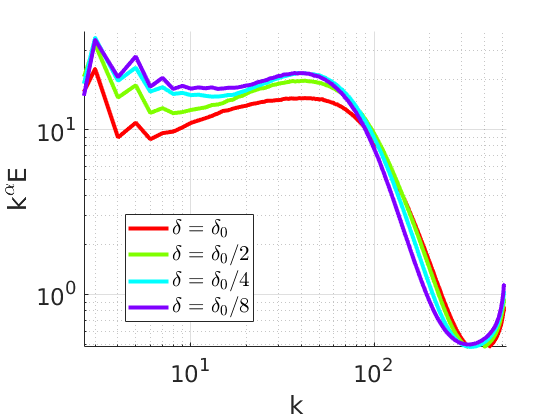
As indicated in Figure 1 (B), a convenient way to check the scaling assumption 4.8 in practice is to consider the compensated energy spectrum, which is defined as , where is the (proposed) scaling exponent in the inertial range. proposition 4.9 says that if there exists , such that the compensated energy spectrum is uniformly bounded by a constant, and independently of , then is compact in .
Remark 4.11.
If and , then Kolmogorov’s theory states that for fully developed turbulence . Based on our estimate, this requires . So that the (expected) energy spectrum is . Such an assumed scaling is consistent with many real, as well as numerical, experiments reported in the literature, and is sufficient for compactness in the space of probability measures (cp. proposition 4.9).
4.5. Lax-Wendroff type theorem
We have used a compactness argument to show that under some reasonable hypotheses on the approximations, numerical solutions computed by the spectral hyper-viscosity converge to a limiting time-parametrized probability measure. In this section, we show that such a limit necessarily is a statistical solution of the incompressible Euler equations in the sense of definition 3.1.
Theorem 4.12 (Lax-Wendroff type theorem).
Let be computed by the spectral hyper-viscosity scheme with initial data , and assume in , as . Then is a statistical solution of the incompressible Euler equations with initial data .
Proof.
Fix . Let be given solenoidal test functions. Set and denote . Let be obtained from the spectral method, with initial data . Let us denote . Then, as a consequence of lemma 4.3, we can write
where there exists independent of and the initial data , such that the error term satisfies . Taking the product over , we find
where . Recognizing the special structure of the empirical measure (33) as a convex combination, denoting by the k-point correlation measure corresponding to , we obtain from the above identity that,
| (40) |
The right-hand side can be bounded by
which, by lemma 4.3 is further bounded by
Note that if is supported on , then it follows that is supported on , as well. This is a consequence of the a priori -bound (32). Hence the error term in equation (40) is in this case bounded by , where is a constant independent of .
Let us also note that the terms on the left-hand side of (40) converge strongly in as . Indeed, it is not difficult to see that all terms on the left -hand side, e.g.
are admissible observables in the sense of (18). For such observables, the -convergence of
has been established in theorem 2.12. The same holds true for the other two terms on the left-hand side.
Passing to the limit , it thus follows that
The fact that is concentrated on incompressible vector fields follows immediately from the corresponding property of the approximations (cp. lemma 3.3). Furthermore, from proposition 2.9, it also follows that the limit is time-regular. This finishes the proof that is a statistical solution of the incompressible Euler equations with initial data . ∎
5. Numerical Experiments
In this section, we will present a suite of numerical experiments to demonstrate the effectiveness of the Monte Carlo algorithm 4.1 in computing statistical solutions of the incompressible Euler equations.
5.1. Implementation
For our numerical experiments, we use the implementation of the spectral hyper-viscosity scheme (28) provided by the SPHINX code, which was first presented in [24]. In SPHINX, the non-linear advection term is implemented using the -costly fast Fourier-transform. Aliasing is avoided via the use of a padded grid, as e.g. described in [24, 23]. The spectral scheme is implemented based on the primitive variable formulation.
For the numerical experiments reported below, we use a spectral viscosity operator of order (cp. equation (28)), with , unless otherwise stated. The Fourier multiplier is chosen with Fourier coefficients
corresponding to .
For each sample, SPHINX solves the following system of ODEs for the Fourier coefficients , of :
| (41) |
for , . Here denote the Fourier coefficients of the initial data. The multiplication by the matrix implements the Leray projection onto divergence-free vector fields. The dot product with corresponds to taking the divergence in Fourier space. We note that the -th Fourier component of is constant in time, reflecting conservation of momentum. In SPHINX, this component is set equal to . The above system of ODEs (41) is integrated in time using an adaptive explicit third-order Runge-Kutta method.
Although the theory of section 4 is valid for both two and three space dimensions and the SPHINX code is available for both cases, we restrict our focus to two space dimensions in this section, on account of affordable computational costs.
5.2. Flat Vortex Sheet.
Vortex sheets occur in many models in physics and are an important test bed for numerical experiments for the Euler equations [22] and references therein. We first consider a randomly perturbed version of the flat vortex sheet that corresponds to the following initial data also considered in [22],
5.2.1. Initial data
Given a smoothing parameter , and a parameter (measuring the size of the random perturbation of the interface), this vortex sheet initial data is of the form
| (42) |
where denotes the Leray projection, is the following smoothened flat vortex sheet initial data:
and is a random function, which for a given (random) choice of parameters , , is defined by
| (43) |
We will also consider the discontinuous case of initial data that are obtained in the limit resulting in
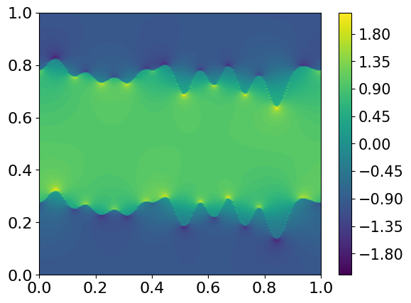
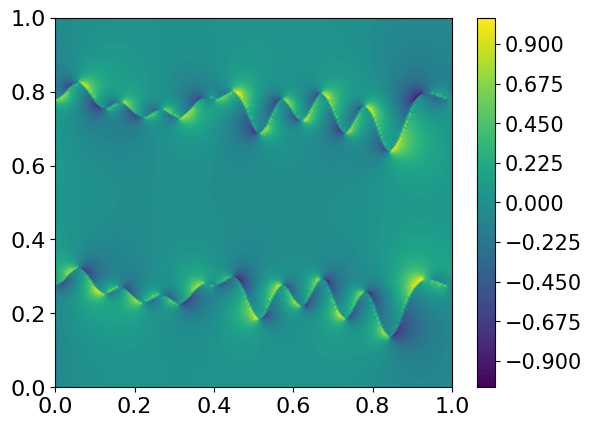
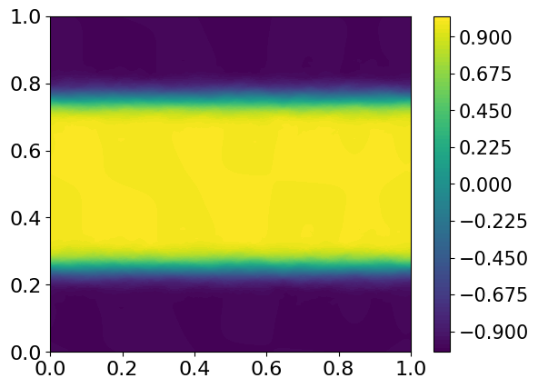
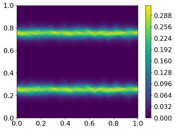
For our simulations, we fix modes for the perturbations. The coefficients are drawn independently, uniformly in , and then multiplied by . The coefficients are i.i.d., with a uniform distribution on . The initial data for the statistical solution is defined as the law of these random perturbations. It depends on the two parameters , . While controls the smoothness of the initial data, measures the amplitude of the perturbation. We fix in the following and consider different values of . Note that the choice corresponds to an initial measure supported on discontinuous flows with a very sharp transition (see figure 2 (A,B) for realizations (samples) of this initial data). In figure 2 (C,D), we present the initial mean and variance that correspond to the random variations of the initial interface location.
Clearly when , the corresponding initial data for every sample is smooth. Consequently, smooth solutions of (1) are well-posed and the spectral viscosity method converges to this solution as [2]. However for , which corresponds to the case of a discontinuous vortex sheet, there are no well-posedness results even for weak solutions, as the vorticity corresponding to the initial datum (for each sample) is a sign changing measure and does not belong to the Delort Class. In [22], the authors had presented multiple numerical experiments to illustrate the approximate solutions, computed with a spectral viscosity method, may not converge (or converge too slowly to be of practical interest) for individual samples (see figures 5 and 6 of [22]). Hence, it would be interesting to study if approximate statistical solutions, generated by algorithm 4.1 converge in this case.
5.2.2. Structure functions and Compensated Energy spectra.
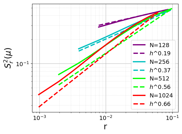
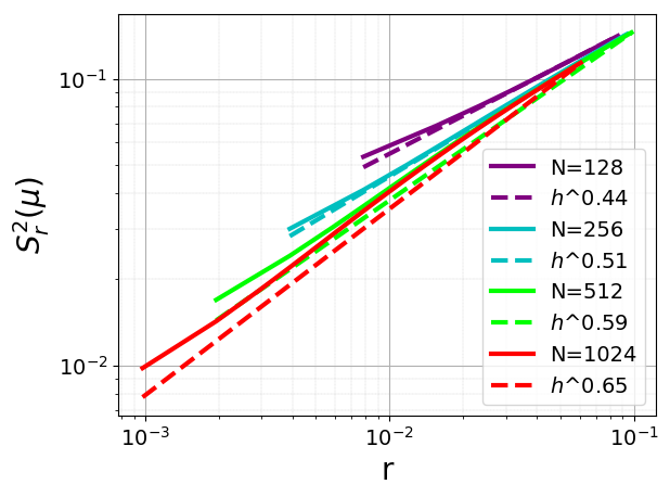
The convergence theorem 4.6, based on the compactness theorem 2.8, provides us with verifiable criteria to check convergence of algorithm 4.1. In particular, we need to check certain decay conditions on the structure function (11) for small correlation lengths. To this end, we consider the following instantaneous version of the structure function (11),
| (44) |
Note that the above is a formal definition and it can be made rigorous in terms of the time-dependent correlation measures. It is much simpler to compute the instantaneous quantity (44) than the time-averaged version (11).
Our objective is to check whether the structure function (11), or rather its instantaneous version (44), decays (uniformly in resolution ) as . Such a decay would automatically imply convergence of the approximations to a statistical solutions by theorems 2.8 and 4.12.
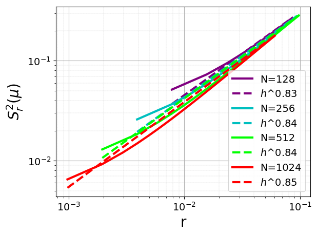
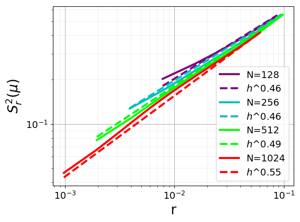
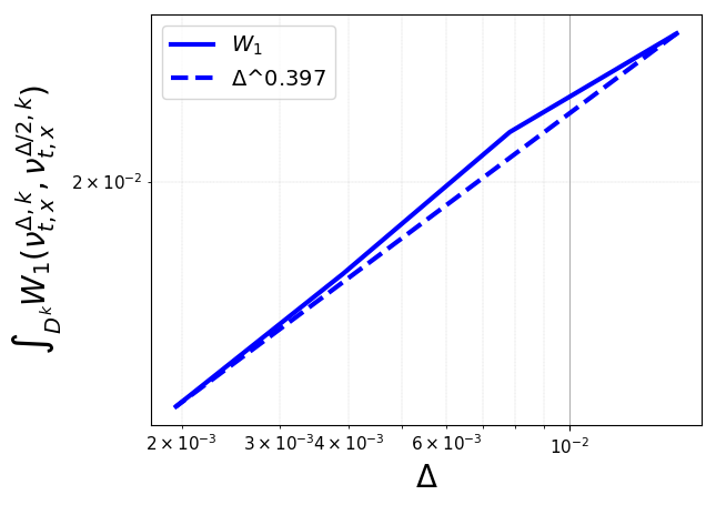
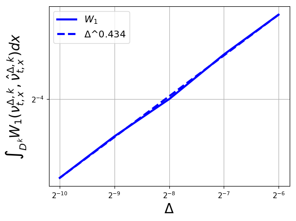
Clearly if in (42), the spectral viscosity method converges to the unique classical solution as . Moreover, a straightforward calculation shows that the structure function (44) should scale as,
| (45) |
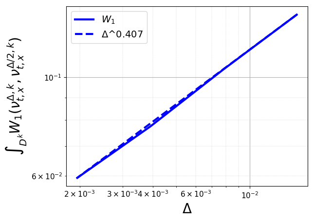
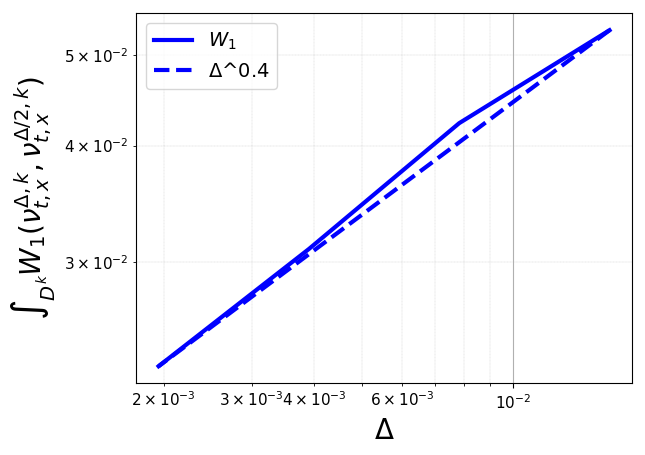
This is indeed verified from figure 3 (A) where we plot the structure function (44) at and for different values of the mesh parameter. We see from this figure that , at fine resolutions, which is very close to the expected value of for the scaling exponent of the structure function.
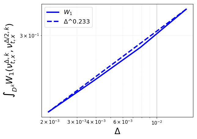
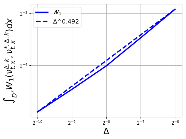
On the other hand, for , corresponding to the discontinuous flat vortex sheet, the lack of smoothness inhibits us from inferring a particular form of decay of (11) (or (44)) a priori.
At least initially, calculations in [21] imply that , for the discontinuous flat vortex sheet. Surprisingly, we find from figure 3 (B) that at fine resolutions, , which agrees with the decay of the structure function of the initial data. Although we do not present the results there, we observe that the structure function (44) scales as , with for all . This implies an uniform decay of the structure function (11) and convergence of the approximations to a statistical solution of the Euler equations (1), even for this case of discontinuous vortex sheet data. Note that the computed structure functions (44) in figure 3 clearly satisfy the approximate scaling hypothesis (37) and thus imply convergence through theorem 4.6.
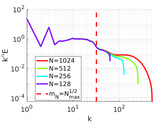
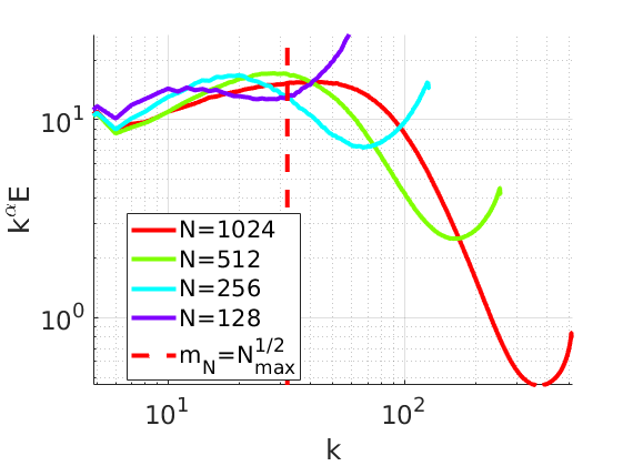
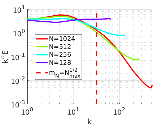
An alternative criterion for convergence of statistical solutions is provided by the energy spectrum decay in the inertial range (38). To check whether this criterion is satisfied, we follow theorem 4.9 and compute the following instantaneous compensated energy spectrum,
| (46) |
Following the arguments in the proof of theorem 4.9, we can relate the decay of the instantaneous energy spectrum to the corresponding decay of the structure function (44) by a direct analogue of (39).
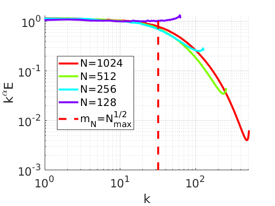
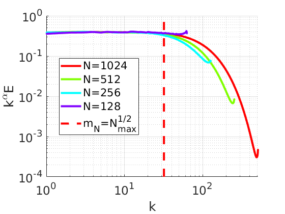
For in (42), we plot the compensated energy spectrum for all and at time , with compensating factor in figure 4 (A). Note that this choice of is consistent with a decay exponent of for the structure function in (39), i.e. . We observe from this figure that as expected for this case, the compensated energy spectrum is clearly bounded and in fact, decays faster than the expected rate for the entire range of wave numbers.
On the other hand, we plot the compensated energy spectrum (46) for the discontinuous flat vortex sheet case, i.e. in (42), in figure 4 (B). In this case, we expect from the structure function computations (see figure 3(B)) that the instantaneous structure function decays with an exponent of . From (39), we see that this corresponds to the choice of as the exponent of compensation in (46). Moreover, in figure 4 (B), we also plot the line corresponding to wave number , which for the spectral viscosity method (28) represents the wave number after which the spectral viscosity is activated and hence, demarcates the separation between inertial and dissipation ranges. We observe from figure 4 (B) that the compensated energy spectrum is clearly uniformly bounded (in terms of the resolution ) for the whole inertial range and for all resolutions barring the coarsest resolution, and decays fast in the dissipation range, although there is a slight kink upwards at the very end of the dissipation range, almost at the grid scale. This might be attributed to numerical errors, which are dominant at this range. Translating these results to the energy spectrum, we see that the spectrum decays as in the inertial range uniformly with respect to resolution. Hence, according to theorems 4.9 and 4.12, the sequence of approximations will converge to a statistical solution of (1).
5.2.3. Convergence in Wasserstein Metrics.
Given the computational results on the structure function and the compensated energy spectra, results in section 4 clearly imply convergence of the approximations , generated by the Monte Carlo algorithm 4.1 to a statistical solution of the incompressible Euler equations. Moreover from the discussion in section 2, we should observe with respect to the following Cauchy rates:
| (47) |
Unfortunately, the calculation of the Wasserstein distance between probability measured defined on high-dimensional (or indeed -dimensional) spaces is a highly non-trivial issue, which we cannot tackle with present computational resources.
On the other hand, one can compute finite-dimensional marginals of (47) by utilizing the complete characterization of in terms of correlation measures as given in theorem 2.11. Following [14] (theorem 5.7), one can prove that,
| (48) |
Here, and is the -th correlation marginal corresponding to the approximate statistical solution . Note that we consider instantaneous versions of the Wasserstein metric (47) for reasons of computational convenience.
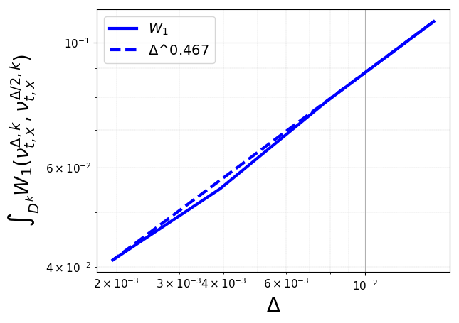

We remark that computing the Wasserstein distances for small is much more tractable. We have computed these Wasserstein distances using the algorithm of [5] (as implemented in [17]) and the corresponding results for , at time for the discontinuous flat vortex sheet, i.e. in (42) are presented in figure 5. As seen from this figure, we observe a clear convergence of these Wasserstein distances (in the Cauchy sense as in (48)) for the one-point, two-point and three-point correlation measures, albeit at a slow rate for the second and third correlation marginals. This, together with the results on the structure function and compensated energy spectra, provides considerable evidence that the approximate statistical solutions, generated by algorithm 4.1, converge to a statistical solution of (1). Moreover, given theorem 2.12, results shown in figure 5 establish convergence with respect to any admissible observable in the sense of (18), corresponding of one-point, two-point and three-point statistical quantities of interest. These include mean, variance, structure functions, energy spectra as well as three-point correlation functions.
5.3. Sinusoidal vortex sheet
In this section, we will consider a random perturbation of the so-called sinusoidal vortex sheet, i.e. the initial vorticity is concentrated on a sine curve. This test case was extensively studied in a recent paper [23] in the context of numerical approximation of weak solutions (in Delort class) of the two-dimensional incompressible Euler equations.
5.3.1. Initial Data.
We fix a sinusoidally perturbed vortex sheet, where the initial vorticity is a Borel measure of the form
such that , and up to a constant, is uniformly distributed along a curve , which is defined as the graph:
We chose for our simulations.
The numerical initial data is obtained from the mollification of this initial data with a parameter . As a mollifier, we consider the third-order B-spline
Next, we define . The numerical approximation of the perturbed vortex sheet is now defined by setting
where determines the thickness (smoothness) of the approximate vortex sheet. The convolution at is evaluated via numerical quadrature:
with equidistant quadrature points in , and the function whose graph is , i.e. . We choose quadrature points. We denote by the velocity field such that and .
Similar to the case of the flat vortex sheet, we carry out random perturbations of the sinusoidal vortex sheet as follows:
Here, denotes the Leray projection onto divergence-free vector fields, and we again fix a random function ,
depending on a parameter and a choice of (random) coefficients , . For our simulations, we fix modes for the perturbations. In practice, the coefficients are first drawn independently, uniformly in , and then multiplied by . The coefficients are i.i.d., with a uniform distribution on . The initial data for the statistical solution is defined as the law of these random perturbations. It depends on the two parameters , . While controls the smoothness of the initial data, measures the amplitude of the perturbation. We fix in the following and vary as a function of the grid size . To approximate vortex sheet initial data, we must scale with , such that as . We use for our simulations. The additional diffusion parameter of the spectral viscosity scheme is set to . With this choice of parameters, we will drop the sub- and superscripts and denote the initial data at a given resolution simply by .
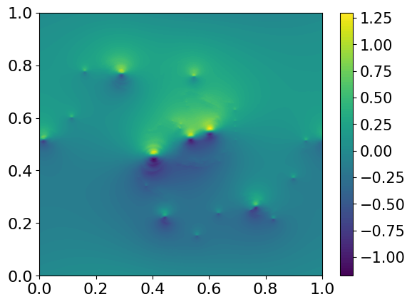

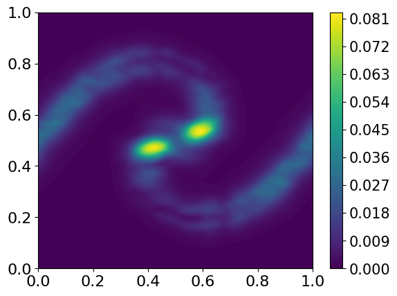
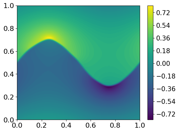
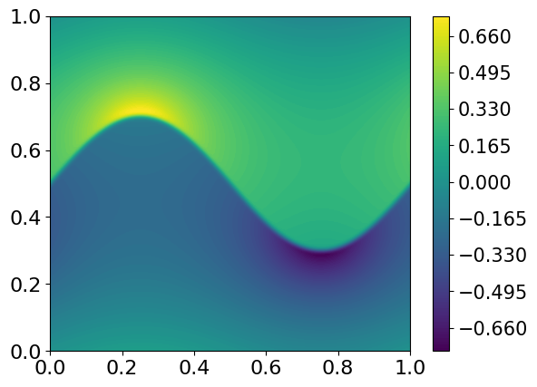
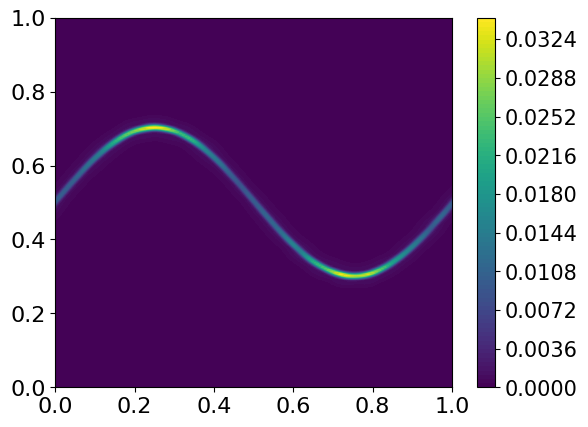
5.3.2. Computation of individual samples
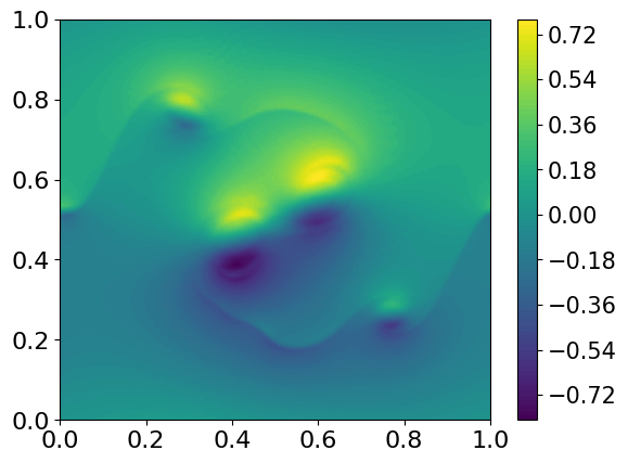
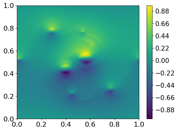
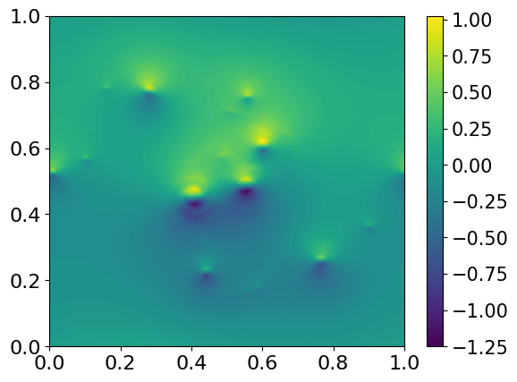
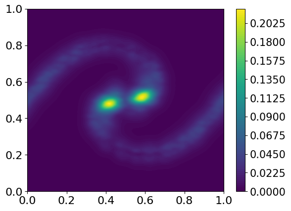
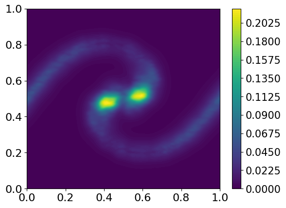
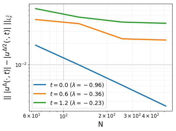
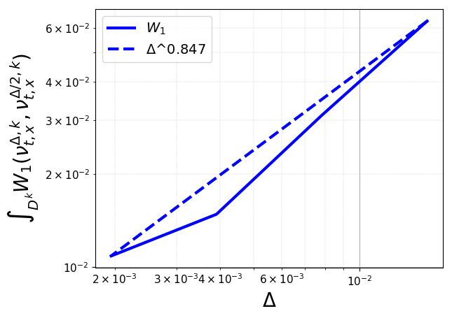
For any single realization of the random perturbation , the resulting vorticity of the initial datum (sample) is a positive measure, concentrated on a sine curve (see figure 6 (A) for horizontal component of velocity ). Hence, any single sample of the initial data in the Delort class. Therefore, by the results of [23], the approximate solutions generated by the spectral viscosity method (28) will converge, on increasing resolution, to a weak solution of (1). However, as noted in [23], this convergence can be very slow as the flow breaks down into smaller and smaller vortices. In fact, this phenomenon is also seen from figure 7 (Top row), where we plot the horizontal component of velocity at time and different resolutions. At this time, the initial vortex sheet has rolled over and broken down into a succession of small vortices, whose location and amplitude are different for different resolutions. This very slow convergence is also displayed in figure 8 (A), where we plot the Cauchy rates , with denoting the approximate solution computed with the spectral viscosity method (28), for three different times . As seen from this figure, the rate of convergence decreases very rapidly and at time , it appears as if there is no convergence on mesh refinement.
5.3.3. Structure functions and Compensated energy spectra.
Given this apparent non-convergence of individual samples, it is pertinent to investigate if computing the statistics will be more convergent. To this end, we consider the initial data to be the initial probability measure . The mean and variance (of the horizontal component ) are plotted in figure 6 (B,C). From this figure, we observe that the initial probability measure is concentrated on very small perturbations of the underlying sinusoidal vertex sheet, as reflected in the initial variance.
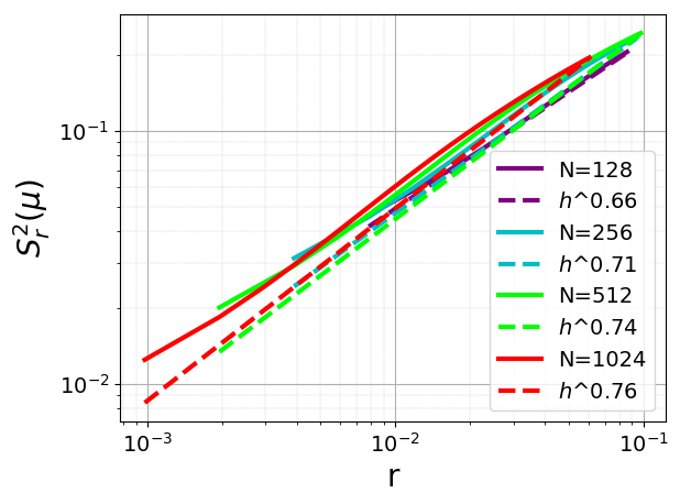
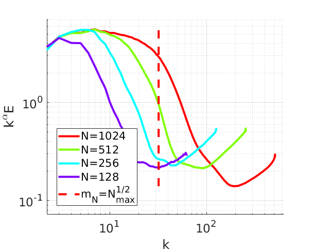
In order to investigate the convergence of approximations to the statistical solution, generated by the algorithm 4.1, we follow the template of the previous numerical experiment and compute the (instantaneous) structure function (44) and the compensated energy spectrum (46) in figure 9. From this figure, we observe that the structure function at time scales with an exponent of at the finest resolutions. From (39), this implies roughly a in the scaling of the energy spectrum (46). A better fit to the scaling of the energy spectrum is found with . We plot the compensated energy spectrum with the latter value of in figure 9 (B). From this figure, we see that for the inertial range, the energy spectrum clearly decays (faster than) a rate of . Thus, the assumptions of theorems 2.8, 4.9 are satisfied and the approximations will converge to a statistical solution of (1).
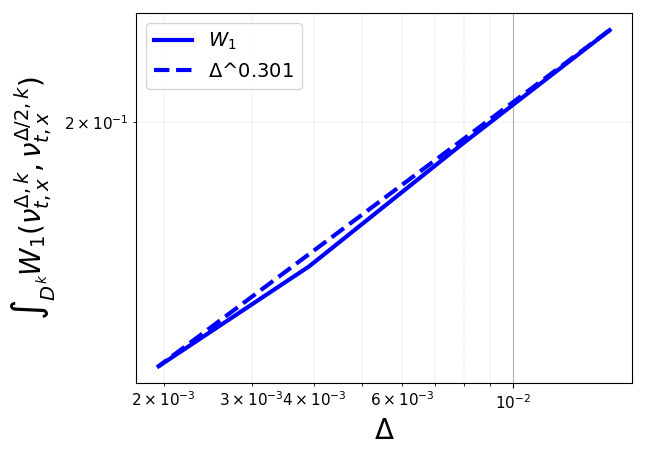
5.3.4. Convergence of observables and Wasserstein Distances.
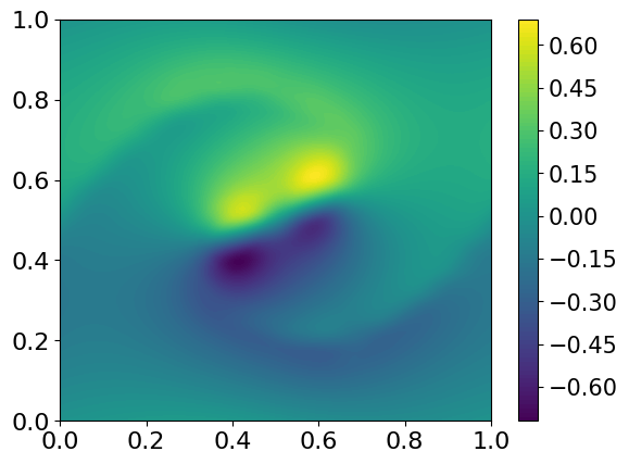
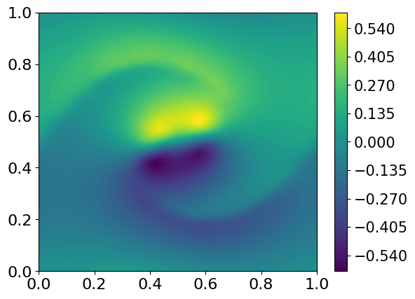
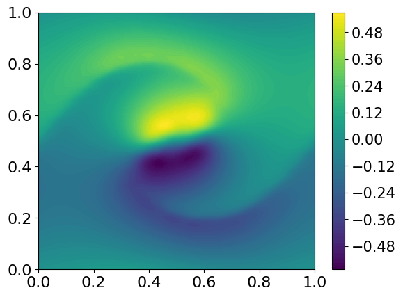
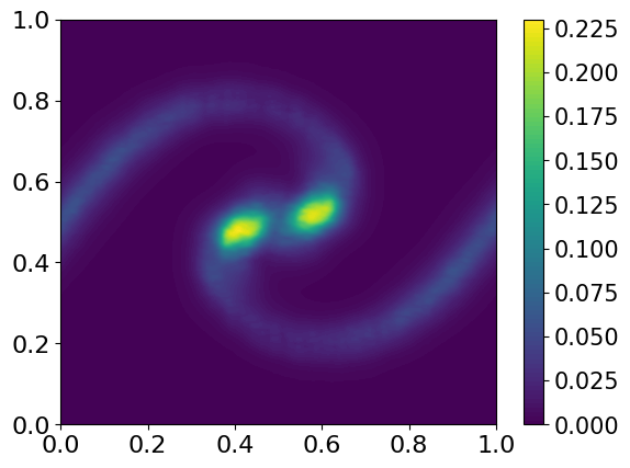
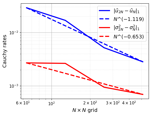
Given the results on the computed structure functions and energy spectra, the approximations will converge. But is this convergence at a better rate than that of single samples? To investigate this issue, we consider two different sets of computations. First, we compute the mean and the variance of the velocity field at different resolutions and plot them (for the horizontal velocity at time in figure 7 (Middle and Bottom rows). Clearly, the one-point statistics appear much more convergent than the single sample results. The mean flow consists of a coherent set of large vortices, which is in stark contrast to the large number of vortices formed in the single sample simulations. Moreover, we also plot Cauchy rates for the mean and the variance, corresponding to the norm at time , and different resolutions in figure 8 (B). Again, we observe that these one-point statistics converge at a significantly faster rate than the single sample. These results indicate that one can expect significantly better convergence of approximations for statistics than for individual realizations of fluid flows, even if the initial probability measure is a small perturbation of the underlying deterministic data and further reinforces the results of [11, 22, 14] in this direction.

Finally, we plot the Wasserstein distances (48) for , corresponding to the one- and two-point correlation marginals, at time , in figure 10. The results clearly show convergence in these metrics at a significantly faster rate than for individual samples and indicate possible convergence in the metric (9) on probability measures on .
5.4. Fractional Brownian Motion.
The study of the evolution of initial ensembles corresponding to (fractional) Brownian motion stems from [43, 45], where the authors model interesting aspects of Burgers turbulence by evolving Brownian motion initial data for the (scalar) Burgers’ equation, see [13] for a more recent numerical study. Similarly in [14], the authors consider the compressible Euler equations with (fractional) Brownian motion initial data. Following these articles, we will consider the two-dimensional Euler equations (1) with initial data corresponding to fractional Brownian motion, i.e. the following initial data:
| (49) |
where and are two independent two-dimensional fractional Brownian motions with the Hurst index . Standard Brownian motion corresponds to a Hurst index of . The initial probability measure is the law of the above random field.
To generate fractional Brownian motion, we use the random midpoint displacement method originally introduced by Lévy [27] for Brownian motion, and later adapted for fractional Brownian motion, see [14] section 6.6.1.
Considering fractional Brownian motion initial data (49) is a significant deviation from the vortex sheet initial data in the following respects,
-
•
For the vortex sheet initial data, the initial measure was concentrated on a 20-dimensional subset of (corresponding to the choice of 20 free parameters , ). On the other hand, in the limit of infinite resolution (), the fractional Brownian motion initial data corresponds to a measure concentrated on an infinite dimensional subset of .
-
•
For any , and for any sample , the initial vorticity for (49) is not a Radon measure. Consequently, the initial data does not belong to the Delort class and there are no existence results for the corresponding samples. Hence, fractional Brownian motion does not fall within the ambit of any of the available well-posedness theories for two-dimensional Euler equations.
-
•
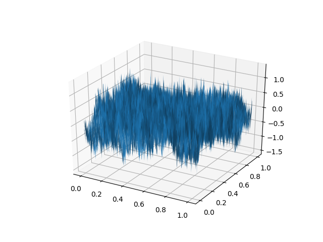
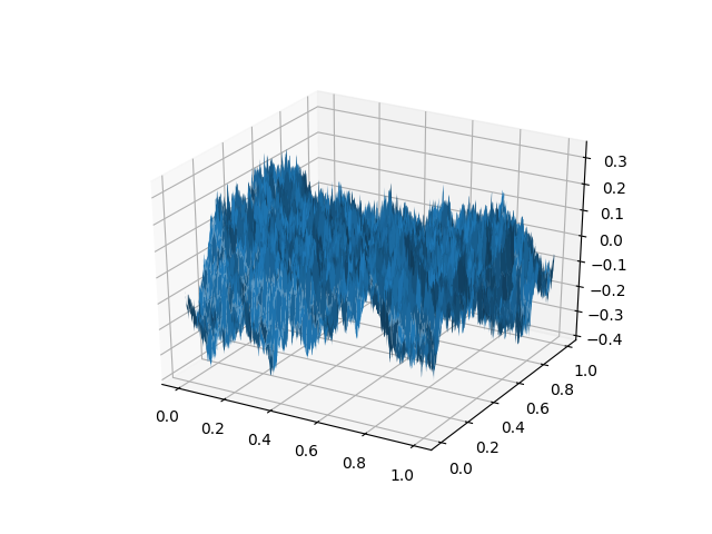
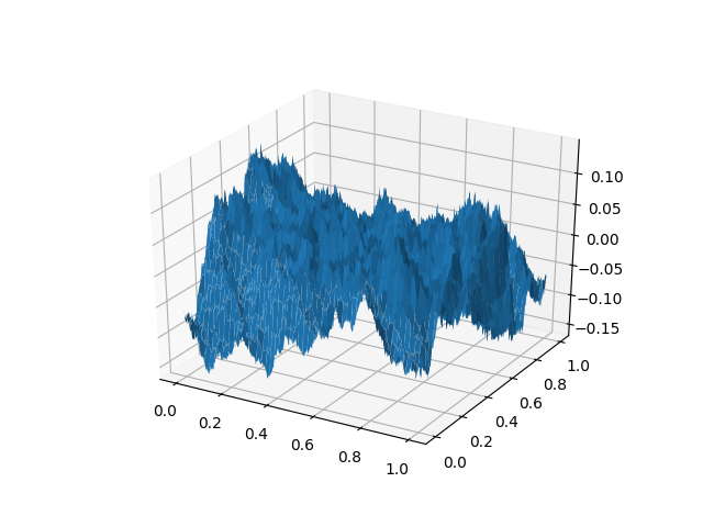
The Hurst index in (49) controls the regularity (and also roughness) of the initial data (pathwise). Roughly speaking, each sample is Hölder continuous with exponent . Hence, we can consider a very wide range of scenarios in terms of roughness of the initial data by varying the Hurst-index , see figure 11 for realizations of the horizontal velocity field for three different Hurst indices. In particular, one can observe from this figure that lowering the value of leads to oscillations of both higher amplitude and frequency in the initial velocity field.
5.4.1. Structure functions and Compensated energy spectra
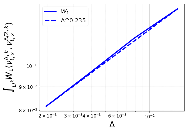
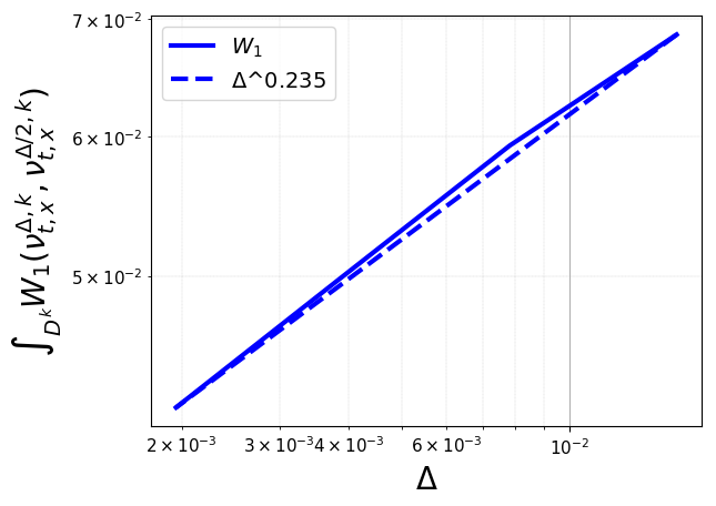
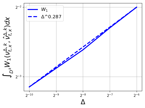
In order to verify convergence of the approximations, generated by algorithm 4.1, for the fractional Brownian motion initial data (49), we will check if the computed structure functions (44) decay uniformly with respect to resolution, on decreasing correlation lengths. In figure 12 (Top Row), we plot the structure function at time for three different Hurst indices of and observe that the structure functions indeed decay to zero at a certain exponent (independent of resolution). These exponents are approximately for initial , for the standard Brownian motion initial data () and for the initially rough . These results indicate that the conditions of the compactness theorem 2.8 are fulfilled and the approximations converge to a statistical solution of (1).
This convergence is further reinforced by the computed compensated energy spectra (46), at time , for the three different Hurst indices shown in figure 12 (Bottom Row). Based on the value of the Hurst index, we choose the compensating index for the ,,, respectively. These values of are chosen to provide the correct scaling of the energy spectra at the initial time . As seen from figure 12, the compensated energy spectra remain bounded up to the final time , independent of the spectral resolution. Hence, the energy spectrum decays at least at the rate of for increasing wave number , in the inertial range. Consequently, we can readily apply proposition 4.9 and conclude that the approximations, generated by the algorithm 4.1, converge to a statistical solution, for all three values of the Hurst index in (49).
5.4.2. Convergence in Wasserstein distance.
Next, we seek to verify convergence of observables (statistical quantities of interest). To this ends, we follow the previous section and compute the Wasserstein distances , corresponding to the -point correlation marginals for the three different Hurst indices of . In figure 13, these metrics are computed at time , for , corresponding to one-point and two-point statistical quantities of interest. As observed from the figure, the approximations clearly converge in this metric for both one- and two-point statistics, at rates which are independent of the underlying initial Hurst index. The two-point correlation marginals appear to converge at a slower rate than the one-point Young measures. These results validate convergence of all one- and two-point statistical quantities of interest. Taken together with the results for the structure function, compensated energy spectra and theorem 2.8, they strongly suggest convergence in metric (9) on .
5.5. Stability of the computed statistical solution.
The afore-presented numerical experiments clearly validate the convergence theory developed in this article. Therefore, algorithm 4.1 provides a practical way to compute statistical solutions. We use this algorithm to study the sensitivity/stability of the computed statistical solution in the context of the discontinuous flat vortex sheet initial data ( in (42)) to the following perturbations,
-
•
Type of the initial perturbation, with respect to the underlying probability distribution.
-
•
Type of underlying numerical method.
-
•
Amplitude of the initial perturbation.
We start by changing the type of the underlying initial probability measure in the flat vortex sheet initial data. Instead of choosing the i.i.d. random variables according to a uniform distribution as before in (42), we choose them from a normal distribution with mean and variance . The mean and variance are chosen so the distribution’s mean and variance are consistent with those of .

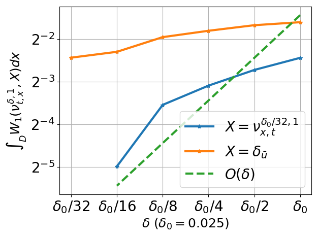
In order to compare the corresponding approximate statistical solutions, we compute the Wasserstein distance , at different resolutions . Here, is the statistical solution computed with normally distributed initial data and is the corresponding correlation measure. We set the initial perturbation amplitude in (42), and and plot the computed Wasserstein distances in figure 14 (Left column). As seen from this figure, the two approximate solutions clearly converge to each other in this metric as the resolution is increased. This indicates that the computed statistical solutions are stable with respect to the variation of underlying initial probability measures.
Next, we consider if the computed statistical solution depends on the underlying numerical method. To this end, we compute the statistical solution for the discontinuous flat vortex sheet initial data (42) with algorithm 4.1 but replace the spectral viscosity method with a finite difference projection method [7, 3, 24]. The convergence of this method to a statistical solution is considered in a forthcoming paper [38]. We denote the computed statistical solutions with this method as and the corresponding correlation measures as and compute the Wasserstein distance at time and and plot the results in figure 14 (Right Column). From this figure, we readily conclude that the statistical solutions computed with the finite difference projection method converges to that computed with the spectral viscosity method on increasing resolution. This strongly suggests the stability of the computed statistical solutions to the underlying (convergent) numerical method.
Finally, we compute approximate statistical solutions for different amplitudes of the initial (random) perturbation in (42) by taking different values of the perturbation amplitude ranging from to , corresponding to smaller and smaller perturbations of the underlying flat vortex sheet. We computed the statistical solution at the highest resolution of with Monte Carlo samples in algorithm 4.1.
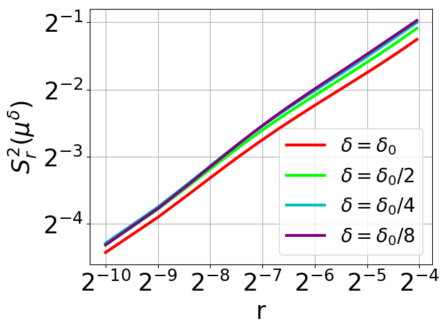
First, we examine if there is convergence of the computed statistical solutions as . To this end, we compute the instantaneous structure function (44) at time for different values of and plot the results in figure 15 (Top Row, Left). Clearly, the computed structure functions are very close and decay with decreasing correlation length with approximately the same exponent. Thus, we can appeal to theorem 2.8 and claim that the approximate statistical solutions converge. This is further reinforced when we compute the instantaneous compensated energy spectrum (39) at time and with . We observe from figure 15 (Top Row, Right) that the computed energy spectra with different values of are very close and decay at the approximately the same rate. Hence, from theorem 4.9, the underlying approximate statistical solutions will converge.
After establishing convergence of statistical solutions when the amplitude of perturbations in the initial datum (42) is decreased, it is natural to ask what these solutions converge to. One possibility is the initial discontinuous flat vortex sheet itself. After all, setting in (42), it is easy to see that the discontinuous flat vortex sheet is a stationary solution of the incompressible Euler equations. To check if this stationary solution is indeed the zero perturbation limit of the computed statistical solution, we compute the Wasserstein distances and for different values of the perturbation parameter with and . Here, is the stationary solution corresponding to the flat vortex sheet initial data, i.e. . We display these distances in figure 15 (Bottom Row). We observe from this figure that there does not seem to be any perceptible evidence of convergence to the stationary solution. This is consistent with the findings in [22], where the authors had observed a non-atomic measure-valued solution as the limit of the perturbations to the flat vortex sheet.
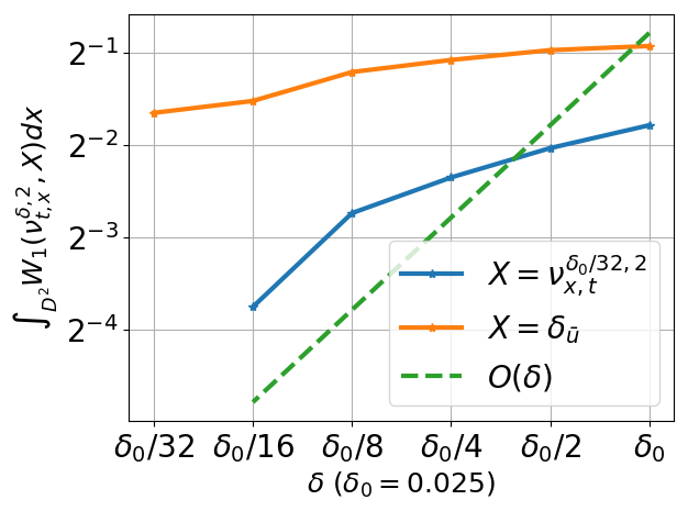
In order to further identify the limit of the computed statistical solutions as , we compute a reference solution , by setting in (42) and as the spectral resolution and Monte Carlo samples. We compute the Wasserstein distances for different values of the perturbation parameter with and . Here, is the correlation measure, corresponding to the reference statistical solution. The distances, plotted in figures 15 (Bottom Row), do decrease as is decreased, albeit at a slow rate. However, this decrease is clearly visible when compared to the lack of convergence to the stationary solution in the same figures. Thus, we have established that the computed statistical solutions are stable with respect to the amplitude of perturbations and moreover, converge to a probability measure that is different from the one concentrated on the stationary solution.
6. Discussion
We consider the incompressible Euler equations (1) in this paper. The existence of classical (or weak) solutions is an outstanding open question in three space dimensions. Although weak solutions are known to exist in two space dimensions, even for very rough initial data, they may not be unique. Similarly, numerical experiments reveal that standard numerical methods may not converge, or converge very slowly, to weak solutions on increasing resolution.
Given these inadequacies of traditional notions of solutions, it is imperative to find solution concepts for (1) that are well-posed and amenable to efficient numerical approximation. In this context, we consider the solution framework of statistical solutions in this paper. Statistical solutions are time-parametrized probability measures on . Given the characterization of probability measures on spaces in [12], these measures are equivalent to so-called correlation measures, i.e. Young measures on tensor-products of the underlying domain and phase space that represent multi-point spatial correlations. Furthermore, we require statistical solutions to satisfy an infinite number of PDEs (see definition 3.1) for the moments of the underlying correlation measure. Hence, a statistical solution can be interpreted as a measure-valued solution (in the sense of [10]), augmented with information about the evolution of all possible multi-point spatial correlations.
Our aim in this paper was to study the well-posedness and efficient numerical approximation of statistical solutions. To this end, first, we had to characterize convergence on a weak topology on the space , under an assumption of time-regularity on the underlying measures. Convergence in this topology amounted to convergence of a very large class of observables (or statistical quantities of interest). We then proposed a notion of dissipative statistical solutions and also proved well-posedness results for them in a generic sense, namely when the initial measure is concentrated on functions sufficiently near initial data for which smooth solutions exist. This led to short-time well-posedness if the initial probability measure is concentrated on smooth functions. In two space dimensions, we proved global well-posedness for statistical solutions when the initial data is concentrated on smooth functions. Moreover, we also proved a suitable variant of weak-strong uniqueness.
Our main contribution in this paper is the proposal of an algorithm 4.1 to approximate statistical solutions of the Euler equations. This Monte Carlo type algorithm is a variant of the algorithms proposed recently in [11, 22, 14] and is based on an underlying spectral hyper-viscosity spatial discretization. Under verifiable hypotheses, we prove that the approximations converge in our proposed topology to a statistical solution. These hypotheses either rely on a suitable scaling (or uniform decay) for the structure function, or equivalently, on finding an inertial range (of wave numbers) on which the energy spectrum decays (uniformly in resolution). These hypotheses are very common in the extensive literature on turbulence (see [19] and references therein). A key novelty in this article is the rigorous proof of the fact that easily verifiable conditions on the structure functions or energy spectrum imply a rather strong form of convergence for (multi-point) statistical quantities of interest. For instance, we observe a surprising fact that a bound on the compensated energy spectrum (46) implies that k-point statistics of interest, even for large , converge. The convergence results also provide a conditional global existence result for statistical solutions in both two and three space dimensions.
We present results of several numerical experiments for the two-dimensional Euler equations. From the numerical experiments, we observe that
-
•
Our convergence theory is validated by all the numerical experiments. The assumptions on the structure functions and energy spectra appear to be very clearly fulfilled in practice. Moreover, the computed solutions converge to a statistical solution in suitable Wasserstein metrics on multi-point correlation marginals. In particular, all admissible observables of interest such as mean, variance, higher moments, structure functions, spectra, multi-point correlation functions, converge on increasing resolution and sample augmentation.
- •
-
•
For our numerical examples, we observe convergence of approximations even when the initial data was quite rough such as when the initial vorticity may not have definite sign (as in the flat vortex sheet) or may not even be a Radon measure (as in the fractional Brownian motion with any Hurst index ). For such initial data, the samples are not in the Delort class and the convergence (and existence) theory for two-dimensional Euler equations is no longer valid. On the other hand, we find neat convergence to a statistical solution.
-
•
The computed statistical solutions where observed to be stable with respect to amplitude and type of perturbations of initial data. Moreover, we observed that two very different numerical methods converge to the same statistical solution for a fixed initial data. This is in contrast to the deterministic case, where the computed solutions can differ significantly [24].
Based on the above discussion, we conclude that statistical solutions are a promising solution framework for the incompressible Euler equations. In particular, there is some scope for proving well-posedness results within this class, possibly with further admissibility criteria. Moreover, numerical approximation of statistical solutions is feasible with ensemble averaging algorithms. Statistical solutions can be a suitable framework for uncertainty quantification and Bayesian inversion for the Euler equations and to encode and explain numerous computational and experimental results for turbulent fluid flows.
There are several limitations of the current paper, which provide directions for future work. At the theoretical level, we seek to either relax the criteria on scaling of structure functions or prove it. This will pave the way for global existence results. Similarly, the weak-strong uniqueness results of this paper could be improved.
In terms of numerical approximation, the main issue with the Monte Carlo type algorithm 4.1 is the slow convergence (in terms of number of samples). This necessitates a very high computational cost, particularly in three space dimensions. We plan to consider efficient variants such as multi-level Monte Carlo [13, 37, 25], Quasi-Monte Carlo [34] and deep learning algorithms [35], for computing statistical solutions of the incompressible Euler equations in three space dimensions, in forthcoming papers.
Appendix A Proof of completeness of , Prop. 2.4
Proof of proposition 2.4.
We wish to prove completeness of the metric space . Let be a Cauchy sequence, i.e.
It will suffice to prove that there exists a subsequence with a limit , since then
by the Cauchy property.
We now choose a suitable subsequence (which we shall immediately reindex), by requiring that , for all . It follows that , and thus
is a convergent series in . In particular, this implies that
For a.e. , we thus have that is Cauchy in . Let denote the limit, which is defined a.e. on . To see that is weak- measurable, we note that for any , we have that is measurable, and converges almost everywhere to . It follows that also s measurable. By definition, this means that is weak- measurable.
To show that in , we note that for almost every , we have
Integrating over , it follows that
∎
Appendix B Proof of time-compactness, Thm. 2.8
Lemma B.1.
If is a uniformly time-regular family for which there exists a modulus of continuity , such that
and if there exists , such that
then is -equicontinuous, in the sense that for any , there exists , such that if , then
Proof.
Since is uniformly time-regular, by definition, there exists and , and transfer plans between and , such that
We note that by definition of as the infimum over all transport plans, we have
Integrating in time, we thus find
Our goal is to show that the last term converges to as , uniformly for all . Fix , arbitrary. We want to find , such that implies
| (50) |
Given , let denote mollification with a standard mollifier , supported on a ball of radius around the origin. Then for all ,
together with the fact that and , implies that
Using the decay of the structure function, we have for all :
where the constant . Next, we note that since , it follows from a result originally due to J.L. Lions (cp. [28, p. 59], [29, p. 58, Lemma 5.1], or [44, lemma 8, p.84]) that for any given , there exists a constant such that
| (51) |
Thus, using also that , we can estimate
Using this estimate, and the uniform time-regularity, we find
uniformly in . By assumption, the first term on the right-hand side is bounded by .
Combining these estimates, we find
Given , we can first choose sufficiently small so that . This fixes a value of according to Lions’ estimate (51). Next, we set . It then follows that for , we have
Thus, given , we have found , such that for all , we have (50). This is what we set out to prove, and concludes our proof of the -equicontinuity of . ∎
Next, we note that for any , we can associate to any a , by defining
| (52) |
The expression on the right-hand side is a straight-forward adaption of the Bochner integral for [21]. It is then easy to show that
Fix . Integrating in time over , it follows that
| (53) |
for all sufficiently small . In particular, the following lemma is now immediate from this estimate and lemma B.1:
Lemma B.2.
If is a equicontinuous family, as in the conclusion of lemma B.1, then for any , we can find , such that for any , we have
Thus, the family is a uniform approximation of , in this case.
To show that is relatively compact in , it will thus suffice to prove that is relatively compact, for any given (fixed) . This is a consequence of the following lemmas and the Arzelà-Ascoli theorem.
Lemma B.3.
Let , and fix . Under the assumptions of theorem 2.8, the family is equicontinuous with respect to the -norm, i.e. for any , there exists , such that
Proof.
Fix . Let be given. By assumption on the uniform decay of the structure functions , it follows from lemma B.1 that the are -equicontinuous. Thus, we can find , such that
whenever . Given , we note that for any 1-Lipschitz continuous , we have
Taking the supremum over all -Lipschitz continuous , we conclude that
whenever . Thus, is equicontinuous as an element of . ∎
Lemma B.4.
Let , and fix . Under the assumptions of theorem 2.8, and for any , we have that
is relatively compact.
Proof.
We note that for any , we have
By assumption, there exists a modulus of continuity , such that we have , uniformly for all . It follows that
Furthermore, it is clear from the definition of (cp. eq. (52)), that if for almost all , then also . By theorem 2.2, it now follows that the family is pre-compact in . ∎
We are now in a position to prove theorem 2.8.
Proof of theorem 2.8.
By lemma B.1, the family is equicontinuous in (in the sense made precise in lemma B.1). Then by lemma B.2, the mollifications form a uniform approximation of in the sense of lemma 2.1. By the uniform approximation lemma 2.1, to show that is precompact it therefore suffices to show that for fixed, the set is precompact. As was shown in lemma B.3 and B.4, the mollifications satisfy:
-
•
The mappings are (pointwise) equicontinuous wrt. , with values in the metric space ,
-
•
For each , the set
is precompact.
Since is a complete metric space under the -metric, it follows from the Arzelà-Ascoli characterization of compact subsets of that is precompact in , and hence in particular that is precompact. By the uniform approximation lemma, we conclude that we also have that
is precompact for any .
To conclude the proof, we note that the same argument also applies when time is reversed (or defining the regularization by averaging over the interval , rather than over ). This implies that also
is precompact for any . Combining these results (e.g. setting ), we finally conclude that
is precompact. ∎
Appendix C Proof of existence and uniqueness, Thm. 3.6
We will follow the notation used in section 3.1. Before coming to the proof of theorem 3.6, we observe that
In particular, is covered by the open balls . Since is a separable metric space, we can choose a countable subcovering, i.e. we can find a dense set of initial data in such a way that
| (54) |
Furthermore, choosing such a countable subset for each , , and considering finally the union , we can in fact find a single countable subset of (not depending on ), such that (54) holds for all , .
After this preliminary observation, we now come to the proof of theorem 3.6.
Proof of theorem 3.6.
Let be given, such that . The idea of the proof is to first choose a countable set satisfying (54) for all , and to observe that can be well approximated by atomic measures of the form . We then use the regularity of the solution of the Euler equations with initial data to show that a dissipative solution exists and that it is unique.
Construction of suitable approximants: For any , let us first construct a suitable approximant , of the form
| (55) |
We define the coefficients , as well as a decomposition , recursively as follows: First, denote
| (56) |
such that . Then we set
| (57) |
and inductively
| (58) |
Note that can be thought of as the support of close to , and keeps track of the set that has already been assigned to for some . By this construction, we have
| (59) |
and furthermore
for all . Thus, setting , it follows that
Since is supported in a small neighborhood of , we expect , and it is now natural to define
A dissipative statistical solution with initial data is given by
In the following, we will show that is Cauchy for any , implying the existence of a limit . Since the definition of a dissipative statistical solutions is linear in the probability measure, it is not hard to see that such a limit must itself be a dissipative statistical solution. Furthermore, we will show that the limit has as initial data. Finally, we will show that this is in fact unique in the class of dissipative statistical solutions.
The sequence is Cauchy: Let be arbitrary. Note that
implies that upon defining , we have
Furthermore, the are pairwise disjoint by (59). Thus, setting
we can define a transport plan from to , by
Note that if , then since and , we must in particular have
This implies that
Assuming now wlog that the maximum is , we find from the stability estimate for Lipschitz continuous solutions of the Euler equations that
It follows that
In particular, this shows that is Cauchy , and has a limit .
is a dissipative statistical solutions with initial data : To see this, we first note that the 2-Wasserstein distance between and can be bounded by
Thus, converges to . Since uniformly for , and each is a dissipative statistical solution, this implies that is a statistical solution with initial data .
is unique: Let be any dissipative statistical solution. We have to show that . To this end, we fix for the moment. Since , we have
for all sufficiently large . It will thus suffice to show that can be made smaller than any for large. We now fix , such that . We will from now on denote for . Define a finite convex combination of Dirac measures by
where we set , and . Here, is chosen sufficiently large to ensure that
where is chosen such that . Such exists by assumption on . Note in particular, that for this choice of , we have
for all .
Define now by
Corresponding to this decomposition
and by assumption on the diffusivity of (cp. definition 3.4 on page 3.4), there exists a decomposition of , such that for each :
and
Repeating the argument used in the proof of weak-strong uniqueness for measure-valued solutions [6], it follows from the fact that is a strong solution, that
for almost all , and all . By our choice of , which is supported in and , this implies
for . For , we have instead
by assumption on the -boundedness of .
We conclude that for almost all :
and hence
Since was arbitrary, it follows that for almost all , i.e. is the unique dissipative statistical solution with initial data . ∎
Acknowledgments.
The research of SL and SM is partially supported by the European Research Council Consolidator grant ERC-CoG 770880 COMANFLO.
References
- [1] R. Abgrall and S. Mishra. Uncertainty quantification for hyperbolic systems of conservation laws. Handbook of Numerical Analysis, 18:507–544, 2018.
- [2] C. Bardos and E. Tadmor. Stability and spectral convergence of Fourier method for nonlinear problems: on the shortcomings of the 2/3 de-aliasing method. Numer. Math., 129(4):749–782, 2015.
- [3] J. Bell, P. Collela, and H. M. Glaz. A second-order projection method for the incompressible Navier-Stokes equations. J. Comput. Phys., 85:257–283, 1989.
- [4] V. I. Bogachev. Measure theory. Vol. I, II. Springer-Verlag, Berlin, 2007.
- [5] N. Bonneel, M. van de Panne, S. Paris, and W. Heidrich. Displacement interpolation using Lagrangian mass transport. ACM Trans. Graph., 30(6):158:1–158:12, Dec. 2011.
- [6] Y. Brenier, C. De Lellis, and L. Székelyhidi. Weak-strong uniqueness for measure-valued solutions. Communications in Mathematical Physics, 305(2):351, May 2011.
- [7] A. Chorin. Numerical solution of the Navier-Stokes equations. Math. Comput., 22:745–762, 1968.
- [8] C. De Lellis and L. Székelyhidi, Jr. The Euler equations as a differential inclusion. Ann. of Math. (2), 170(3):1417–1436, 2009.
- [9] J.-M. Delort. Existence de nappes de toubillon en dimension deux. J. Am. Math. Soc., 4(3):553–586, 1991.
- [10] R. J. DiPerna and A. J. Majda. Oscillations and concentrations in weak solutions of the incompressible fluid equations. Comm. Math. Phys., 108(4):667–689, 1987.
- [11] U. S. Fjordholm, R. Käppeli, S. Mishra, and E. Tadmor. Construction of approximate entropy measure valued solutions for hyperbolic systems of conservation laws. Found. Comput. Math., 17(3):763–827, 2017.
- [12] U. S. Fjordholm, S. Lanthaler, and S. Mishra. Statistical solutions of hyperbolic conservation laws I: Foundations. Arch. Ration. Mech. An., 226(2):809–849, 2017.
- [13] U. S. Fjordholm, K. O. Lye, and S. Mishra. Numerical approximation of statistical solutions of scalar conservation laws. SIAM J. Numer. Anal., 56(5):2989–3009, 2018.
- [14] U. S. Fjordholm, K. O. Lye, S. Mishra, and F. Weber. Statistical solutions of hyperbolic systems of conservation law: Numerical approximation. Preprint, available as arXiv:1906.02536v1.
- [15] U. S. Fjordholm, S. Mishra, and E. Tadmor. On the computation of measure-valued solutions. Acta Numer., 25:567–679, 2016.
- [16] U. S. Fjordholm, S. Mishra, and F. Weber. On the vanishing-viscosity limit of the incompressible Navier-Stokes equations. in preparation, 2019.
- [17] R. Flamary and N. Courty. POT Python Optimal Transport library, 2017.
- [18] C. Foias, R. M. Rosa, and R. Temam. A note on statistical solutions of the three-dimensional Navier–Stokes equations: The time-dependent case. Comptes Rendus Mathematique, 348(3):235 – 240, 2010.
- [19] U. Frisch. Turbulence. Cambridge University Press, 1995.
- [20] J. Guzman, C.-W. Shu, and F. A. Sequira. H-Div conforming and DG methods for the incompressible Euler equations. IMA J. Num. Anal., 37:1733–1771, 2017.
- [21] S. Lanthaler. PhD thesis. in preparation, N.D.
- [22] S. Lanthaler and S. Mishra. Computation of measure-valued solutions for the incompressible Euler equations. Mathematical Models and Methods in Applied Sciences, 25(11):2043–2088, 2015.
- [23] S. Lanthaler and S. Mishra. On the convergence of the spectral viscosity method for the incompressible Euler equations with rough initial data. arXiv e-prints, page arXiv:1903.12361, Mar 2019.
- [24] F. Leonardi. Numerical methods for ensemble based solutions to incompressible flow equations. PhD thesis, ETH Zürich, 2018.
- [25] F. Leonardi, S. Mishra, and C. Schwab. Numerical approximation of statistical solutions of planar, incompressible flows. Math. Model Meth. Appl. Sci., 26:2471–2523, 2016.
- [26] D. Levy and E. Tadmor. Non-oscillatory central schemes for the incompressible 2-D Euler equations. Mathematical Research Letters, 4(3):321–340, 1997.
- [27] P. Lévy. Processus stochastiques et mouvement brownien. Les Grands Classiques Gauthier-Villars. [Gauthier-Villars Great Classics]. Éditions Jacques Gabay, Sceaux, 1992. Followed by a note by M. Loève, Reprint of the second (1965) edition.
- [28] J. L. Lions. Equations Differentielles Operationelles. Springer, 1961.
- [29] J. L. Lions. Quelques méthodes de résolutions des problèmes aux limites non linéaires. Dunod, 1969.
- [30] P.-L. Lions. Mathematical topics in fluid mechanics. Vol. 1, volume 3 of Oxford Lecture Series in Mathematics and its Applications. The Clarendon Press, Oxford University Press, New York, 1996. Incompressible models, Oxford Science Publications.
- [31] J.-G. Liu and Z. Xin. Convergence of the point vortex method for 2-D vortex sheet. Math. Comp., 70(234):595–606, 2001.
- [32] J.-G. Liu and Z. P. Xin. Convergence of vortex methods for weak solutions to the -D Euler equations with vortex sheet data. Comm. Pure Appl. Math., 48(6):611–628, 1995.
- [33] M. C. Lopes-Filho, H. J. Nussenzveig-Lopes, and E. Tadmor. Approximate solutions of the incompressible Euler equations with no concentrations. Annales de l’Institut Henri Poincare (C) Non Linear Analysis, 17(3):371 – 412, 2000.
- [34] K. O. Lye. PhD thesis. in preparation, 2019.
- [35] K. O. Lye, S. Mishra, and D. Ray. Deep learning observables in computational fluid dynamics. Preprint, available as arXiv:1903.03040v1.
- [36] A. J. Majda and A. L. Bertozzi. Vorticity and Incompressible Flow. Cambridge Texts in Applied Mathematics. Cambridge University Press, 2001.
- [37] S. Mishra, C. Schwab, and J. Šukys. Multi-level Monte Carlo finite volume methods for nonlinear systems of conservation laws in multi-dimensions. J. Comput. Phys., 231(8):3365–3388, 2012.
- [38] C. Pares-Pulido. Numerical approximation of statistical solutions of the incompressible Euler equations with a finite difference-projection method. in preparation, 2019.
- [39] R.Krasny. A study of singularity formation in a vortex sheet with a point vortex approximation. J. Fluid Mech., 167:65–93, 1986.
- [40] V. Scheffer. An inviscid flow with compact support in space-time. J. Geom. Anal, 3:343–401, 1993.
- [41] A. Schnirelman. Weak solutions with decreasing energy of the incompressible Euler equations. Comm. Math. Phys, 210:541–603, 2000.
- [42] S. Schochet. The rate of convergence of spectral-viscosity methods for periodic scalar conservation laws. SIAM J. Numer. Anal., 27(5):1142–1159, 1990.
- [43] Z.-S. She, E. Aurell, and U. Frisch. The inviscid Burgers equation with initial data of Brownian type. Comm. Math. Phys., 148:623–641, 1992.
- [44] J. Simon. Compact sets in the space . Annali di Matematica Pura ed Applicata, 146(1):65–96, Dec 1986.
- [45] Y. G. Sinai. Statistics of shocks in solutions of inviscid Burgers equation. Communications in Mathematical Physics, 148(3):601–621, Sep 1992.
- [46] E. Tadmor. Convergence of spectral methods for nonlinear conservation laws. SIAM J. Numer. Anal., 26(1), 1989.
- [47] E. Tadmor. Burgers’ equation with vanishing hyper-viscosity. Commun. Math. Sci., 2(2):317–324, 2004.
- [48] M. I. Vishik and A. V. Fursikov. Homogeneous statistical solutions of the Navier-Stokes system. Uspehi Mat. Nauk., 32:179–180, 1977.