Semi-analytical calculation of the singular and hypersingular integrals for discrete Helmholtz operators in 2D BEM

Abstract

Approximate solutions to elliptic partial differential equations with known kernel can be obtained via the boundary element method (BEM) by discretizing the corresponding boundary integral operators and solving the resulting linear system of algebraic equations. Due to the presence of singular and hypersingular integrals, the evaluation of the operator matrix entries requires the use of regularization techniques. In this work, the singular and hypersingular integrals associated with first-order Galerkin discrete boundary operators for the two-dimensional Helmholtz equation are reduced to quasi-closed-form expressions. The obtained formulas may prove useful for the implementation of the BEM in two-dimensional electromagnetic, acoustic and quantum mechanical problems.

1 Introduction

The boundary element method (BEM) is one of the most common numerical techniques to solve elliptic boundary value problems [1, 2]. Making use of the kernel of the considered partial differential equation, integral theorems are employed to express the solution in terms of bounded operators on Sobolev spaces. The Cauchy data of the problem is then obtained by applying an appropriate discretization scheme, which consists in projecting the solution onto finite dimensional trial spaces, and by numerically solving the resulting algebraic equations. Among the possible discretization strategies, the weak formulation known as the symmetric Galerkin method has been largely considered in the literature (see [3] and references therein).

In contrast to the finite element method (FEM), the BEM has the advantage of only requiring the discretization of the boundary of the physical domain without the need to introduce any truncation in open-region problems. However, since most boundary integral operators are singular, regularization procedures must be taken into account. In the present study, a semi-analytical approach is proposed to evaluate all the possible singular integrals arising from the first-order Galerkin discretization of the boundary operators for the two-dimensional Helmholtz equation. These results may be relevant for BEM applications in electromagnetism and acoustics [4, 5] as well as in quantum mechanics [6].

The manuscript is organized as follows. In Section 2, the boundary integral operators are introduced in both their continuous and discrete forms; the two-dimensional Helmholtz kernel derivatives and the linear basis functions are consequently defined. Section 3 is concerned with the calculation of the singular integrals occurring in the discrete single layer operator. In Section 4 and 5, the same analysis is carried out for the discrete double layer operators and for the discrete hypersingular operator, respectively. An alternative approach based on the variational formulation for the hypersingular operator is reported in Section 6. Finally, Section 7 is devoted to the conclusions.

2 Problem statement

Let $g\left(\mathbf{r},\mathbf{r}^{\prime}\right)$ be the kernel of an elliptic partial differential equation over the domain $\varOmega$ and $f\left(\mathbf{r}\right)$ a well-behaved function defined on $S\equiv\partial\varOmega$. The four boundary integral operators known as single layer, double layer, adjoint double layer and hypersingular are defined, respectively, as follows [4, 1]:

$$\hat{S}\left[f\right]\left(\mathbf{r}\right) \equiv\fint_{S}d\mathbf{r}^{\prime}g\left(\mathbf{r},\mathbf{r}^{\prime}\right)f\left(\mathbf{r}^{\prime}\right);$$ (1)

$$\hat{D}\left[f\right]\left(\mathbf{r}\right) \equiv\fint_{S}d\mathbf{r}^{\prime}\frac{\partial g\left(\mathbf{r},\mathbf{r}^{\prime}\right)}{\partial n^{\prime}}f\left(\mathbf{r}^{\prime}\right)=\fint_{S}d\mathbf{r}^{\prime}\nabla^{\prime}g\left(\mathbf{r},\mathbf{r}^{\prime}\right)\cdot\mathbf{n}^{\prime}\,f\left(\mathbf{r}^{\prime}\right);$$ (2)

$$\hat{D}^{\dagger}\left[f\right]\left(\mathbf{r}\right) \equiv\fint_{S}d\mathbf{r}^{\prime}\frac{\partial g\left(\mathbf{r},\mathbf{r}^{\prime}\right)}{\partial n}f\left(\mathbf{r}^{\prime}\right)=\fint_{S}d\mathbf{r}^{\prime}\nabla g\left(\mathbf{r},\mathbf{r}^{\prime}\right)\cdot\mathbf{n}\,f\left(\mathbf{r}^{\prime}\right);$$ (3)

$$\hat{N}\left[f\right]\left(\mathbf{r}\right) \equiv\int_{S}d\mathbf{r}^{\prime}\frac{\partial^{2}g\left(\mathbf{r},\mathbf{r}^{\prime}\right)}{\partial n\partial n^{\prime}}f\left(\mathbf{r}^{\prime}\right)=\int_{S}d\mathbf{r}^{\prime}\nabla\left[\nabla^{\prime}g\left(\mathbf{r},\mathbf{r}^{\prime}\right)\cdot\mathbf{n}^{\prime}\right]\cdot\mathbf{n}\,f\left(\mathbf{r}^{\prime}\right),$$ (4)

where the symbol $\fint$ stands for the Cauchy principal value integral and $\mathbf{n}$, $\mathbf{n}^{\prime}$ are the outward pointing unit normals to $S$ evaluated at $\mathbf{r}$ and $\mathbf{r}^{\prime}$, respectively. A formal solution to the considered elliptic partial differential equation is often provided in terms of (1)-(4). In order to numerically implement these integral operators, a common strategy is to discretize the surface $S$ into a collection of simplices $\left\{S_{n}\right\}$. The unknown solution $f\left(\mathbf{r}\right)$ is then expanded over a set of basis functions defined on specific groups of neighbor simplices. For instance, when the basis functions are a given set of interpolation polynomials $\left\{p_{j}\left(\mathbf{r}\right)\right\}$, we have:

$$f\left(\mathbf{r}\right)=\sum_{j}\alpha_{j}p_{j}\left(\mathbf{r}\right),$$ (5)

with $\alpha_{j}$ representing the value of the function $f\left(\mathbf{r}\right)$ at the $j$-th mesh node. The $j$-th basis function $p_{j}\left(\mathbf{r}\right)$ is defined on the set of simplices $\left\{S_{n}\right\}$ that share the $j$-th mesh node, hereinafter referred to as $\left\{n\in j\right\}$, and vanishes out of its defining domain, so that:

$$\int_{S}d\mathbf{r}^{\prime}p_{j}\left(\mathbf{r}^{\prime}\right)=\sum_{n\in j}\int_{S_{n}}d\mathbf{r}^{\prime}p_{j}^{n}\left(\mathbf{r}^{\prime}\right),$$ (6)

where $p_{j}^{n}\left(\mathbf{r}^{\prime}\right)$ is the restriction of the $j$-th basis function to the $n$-th simplex. According to the well-known Galerkin approach [7, 5], the same set of basis functions may be used to symmetrize the discrete version of the surface integral operators, leading to:

$$S_{ij} \equiv\sum_{m\in i}\,\sum_{n\in j}\int_{S_{m}}d\mathbf{r}\fint_{S_{n}}d\mathbf{r}^{\prime}g\left(\mathbf{r},\mathbf{r}^{\prime}\right)p_{i}^{m}\left(\mathbf{r}\right)p_{j}^{n}\left(\mathbf{r}^{\prime}\right);$$ (7)

$$D_{ij} \equiv\sum_{m\in i}\,\sum_{n\in j}\int_{S_{m}}d\mathbf{r}\fint_{S_{n}}d\mathbf{r}^{\prime}\frac{\partial g\left(\mathbf{r},\mathbf{r}^{\prime}\right)}{\partial n^{\prime}}p_{i}^{m}\left(\mathbf{r}\right)p_{j}^{n}\left(\mathbf{r}^{\prime}\right);$$ (8)

$$D_{ij}^{\dagger} \equiv\sum_{m\in i}\,\sum_{n\in j}\int_{S_{m}}d\mathbf{r}\fint_{S_{n}}d\mathbf{r}^{\prime}\frac{\partial g\left(\mathbf{r},\mathbf{r}^{\prime}\right)}{\partial n}p_{i}^{m}\left(\mathbf{r}\right)p_{j}^{n}\left(\mathbf{r}^{\prime}\right);$$ (9)

$$N_{ij} \equiv\sum_{m\in i}\,\sum_{n\in j}\int_{S_{m}}d\mathbf{r}\int_{S_{n}}d\mathbf{r}^{\prime}\frac{\partial^{2}g\left(\mathbf{r},\mathbf{r}^{\prime}\right)}{\partial n\partial n^{\prime}}p_{i}^{m}\left(\mathbf{r}\right)p_{j}^{n}\left(\mathbf{r}^{\prime}\right).$$ (10)

Let us now focus on the Helmholtz equation over the 2D region $\varOmega\subset\mathbb{R}^{2}$ whose boundary $S$ is a piecewise smooth closed curve. The kernel of the equation is expressed in terms of the Hankel function [8]:

$$g\left(x,y;x^{\prime},y^{\prime}\right)=\frac{i}{4}H_{0}^{(1,2)}\left[k\sqrt{\left(x-x^{\prime}\right)^{2}+\left(y-y^{\prime}\right)^{2}}\right]$$ (11)

and its normal derivatives are given by:

$$\frac{\partial g\left(x,y;x^{\prime},y^{\prime}\right)}{\partial n^{\prime}} =\frac{ik}{4R}H_{1}^{(1,2)}\left(kR\right)\left(\mathbf{R}\cdot\mathbf{n}^{\prime}\right);$$ (12)

$$\frac{\partial g\left(x,y;x^{\prime},y^{\prime}\right)}{\partial n} =-\frac{ik}{4R}H_{1}^{(1,2)}\left(kR\right)\left(\mathbf{R}\cdot\mathbf{n}\right);$$ (13)

$$\frac{\partial^{2}g\left(x,y;x^{\prime},y^{\prime}\right)}{\partial n\partial n^{\prime}} =\frac{ik}{4R^{2}}\left[R\,H_{1}^{(1,2)}\left(kR\right)\left(\mathbf{n}\cdot\mathbf{n}^{\prime}\right)-kH_{2}^{(1,2)}\left(kR\right)\left(\mathbf{R}\cdot\mathbf{n}\right)\left(\mathbf{R}\cdot\mathbf{n}^{\prime}\right)\right],$$ (14)

with $\mathbf{R}\equiv\mathbf{r}-\mathbf{r}^{\prime}=\left(x-x^{\prime},y-y^{\prime}\right)$ and $k$ representing the wave number. The boundary curve $S$ can be discretized into a collection of segments $\left\{S_{n}\right\}$ with lengths $\left\{l_{n}\right\}$ and extrema $\left\{\mathbf{r}_{A}^{n};\>\mathbf{r}_{B}^{n}\right\}=\left\{\left(x_{A}^{n},y_{A}^{n}\right);\>\left(x_{B}^{n},y_{B}^{n}\right)\right\}$, as depicted in Figure 1.

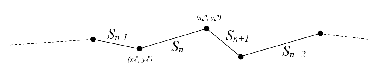
Figure 1: Collection of segments $\left\{S_{n}\right\}$ resulting from the discretization of a 2D curve.

First order basis functions (triangular functions) are defined over pairs of adjacent segments and vary linearly from zero at the outer extrema to unity at the common vertex [7, 5]. By introducing the local variable $t_{n}\in\left[0,1\right]$, which makes it possible to represent an arbitrary point $\mathbf{r}=\left(x,y\right)$ on the $n$-th segment in parametric form:

$$\mathbf{r}\left(t_{n}\right)=\mathbf{r}_{A}^{n}+\left(\mathbf{r}_{B}^{n}-\mathbf{r}_{A}^{n}\right)t_{n},$$ (15)

the restriction of the $j$-th triangular basis function to the $n$-th segment can be written as follows:

$$p_{j}^{n}\left[\mathbf{r}\left(t_{n}\right)\right]\equiv\begin{cases}1-t_{n}&\mathrm{if}\>\mathbf{r}_{j}=\mathbf{r}_{A}^{n};\\ t_{n}&\mathrm{if}\>\mathbf{r}_{j}=\mathbf{r}_{B}^{n},\end{cases}$$ (16)

where $\mathbf{r}_{j}=\left(x_{j},y_{j}\right)$ identifies the coordinates of the $j$-th mesh node.

In the present scenario, each of the discrete operators $S_{ij}$, $D_{ij}$, $D_{ij}^{\dagger}$ and $N_{ij}$ defined in (7)-(10) consists of a sum of four double integrals over the pairs of segments $\left(S_{m},S_{n}\right)\in\left\{m\in i\right\}\times\left\{n\in j\right\}$. A graphical representation of these four terms is reported in Figure 2 for three different choices of the mesh nodes $i$ and $j$.

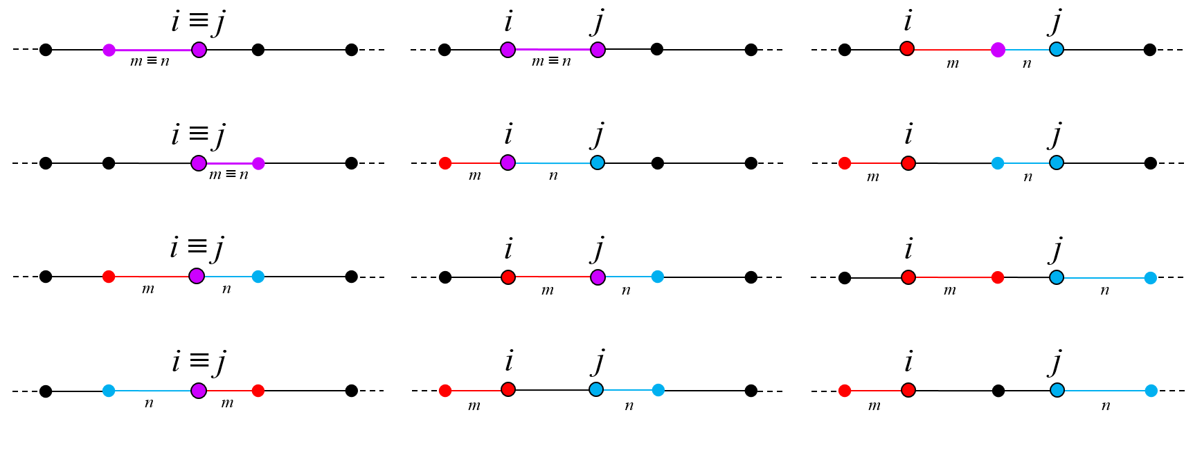
Figure 2: Graphical representation of the four double integrations occurring in each of (7)-(10) when the $i$-th and $j$-th mesh nodes coincide (left column), when they are first neighbors (central column) and when they are second-neighbors (right column). Angles between segments are not displayed here (the reader is referred to Figure 1).

When $S_{m}$ and $S_{n}$ do not share any vertex, all such double integrals can be computed by Gauss-Legendre quadrature rules [8]. The remaining double integrals with $S_{m}=S_{n}$ in (7) and (10) as well as some of the cases where $S_{m}$ and $S_{n}$ share only one vertex (i.e., adjacent segments) are singular and must be treated with due care. In the following, analytical integration formulas will be applied to each of these singular double integrals in order to recast them into a quasi-closed-form expression involving Bessel-related functions and two regular single integrals that can be easily solved numerically.

3 Single layer operator

3.1 Integration over coincident elements

When $S_{m}=S_{n}$, the singular double integrals in (7) are of the form:

$$\frac{i}{4}\int_{S_{n}}d\mathbf{r}\fint_{S_{n}}d\mathbf{r}^{\prime}H_{0}^{(1,2)}\left(k\left|\mathbf{r}-\mathbf{r}^{\prime}\right|\right)p_{i}^{n}\left(\mathbf{r}\right)p_{j}^{n}\left(\mathbf{r}^{\prime}\right),$$ (17)

where the linear functions $p_{i}^{n}\left(\mathbf{r}\right)$, $p_{j}^{n}\left(\mathbf{r}^{\prime}\right)$ are defined in (16) via (15). A useful choice for the reference frames $Oxy$, $O^{\prime}x^{\prime}y^{\prime}$ relative to the two integration coordinates $\mathbf{r}$ and $\mathbf{r}^{\prime}$ is to have both the $x$-axis and the $x^{\prime}$-axis lie along the segment $S_{n}$, with origins $O$, $O^{\prime}$ at $\left(x_{A}^{n},y_{A}^{n}\right)$ and $\mathbf{r}$, respectively (see the left side of Figure 3). With this convention, the $y$ and $y^{\prime}$ coordinates become unnecessary and the integral (17) reduces to:

$$\frac{i}{4}\int_{0}^{l_{n}}dx\fint_{-x}^{l_{n}-x}dx^{\prime}H_{0}^{(1,2)}\left(k\left|x^{\prime}\right|\right)p_{i}^{n}\left(x\right)\widetilde{p}_{j}^{n}\left(x^{\prime},x\right),$$ (18)

where:

$$p_{i}^{n}\left(x\right)\equiv\begin{cases}1-\frac{x}{l_{n}}&\mathrm{if}\>x_{i}=0;\\ \frac{x}{l_{n}}&\mathrm{if}\>x_{i}=l_{n},\end{cases}$$ (19)

$$\widetilde{p}_{j}^{n}\left(x^{\prime},x\right)\equiv\begin{cases}1-\frac{\left(x^{\prime}+x\right)}{l_{n}}&\mathrm{if}\>x_{j}^{\prime}=-x;\\ \frac{\left(x^{\prime}+x\right)}{l_{n}}&\mathrm{if}\>x_{j}^{\prime}=l_{n}-x.\end{cases}$$ (20)

Four kinds of integrals are obtained from (18), (19) and (20), namely:

$$I_{11}^{n} \equiv\frac{i}{4}\int_{0}^{l_{n}}dx\fint_{-x}^{l_{n}-x}dx^{\prime}H_{0}^{(1,2)}\left(k\left|x^{\prime}\right|\right)\left(1-\frac{x}{l_{n}}\right)\left[1-\frac{\left(x^{\prime}+x\right)}{l_{n}}\right];$$ (21)

$$I_{12}^{n} \equiv\frac{i}{4}\int_{0}^{l_{n}}dx\fint_{-x}^{l_{n}-x}dx^{\prime}H_{0}^{(1,2)}\left(k\left|x^{\prime}\right|\right)\left(1-\frac{x}{l_{n}}\right)\left[\frac{\left(x^{\prime}+x\right)}{l_{n}}\right];$$ (22)

$$I_{21}^{n} \equiv\frac{i}{4}\int_{0}^{l_{n}}dx\fint_{-x}^{l_{n}-x}dx^{\prime}H_{0}^{(1,2)}\left(k\left|x^{\prime}\right|\right)\left(\frac{x}{l_{n}}\right)\left[1-\frac{\left(x^{\prime}+x\right)}{l_{n}}\right];$$ (23)

$$I_{22}^{n} \equiv\frac{i}{4}\int_{0}^{l_{n}}dx\fint_{-x}^{l_{n}-x}dx^{\prime}H_{0}^{(1,2)}\left(k\left|x^{\prime}\right|\right)\left(\frac{x}{l_{n}}\right)\left[\frac{\left(x^{\prime}+x\right)}{l_{n}}\right].$$ (24)

The integrals $I_{11}^{n}$ and $I_{22}^{n}$ may be linked to the graphical representations in the second and first row of the left column of Figure 2, respectively. In other words, both $I_{11}^{n}$ and $I_{22}^{n}$ will only arise when the mesh nodes $i$ and $j$ coincide. Similarly, $I_{12}^{n}$ can be associated to the first sketch in the central column of Figure 2, as would be for $I_{21}^{n}$ if we exchanged the node labels: these two integrals come into play when $i$ and $j$ are first neighbors.

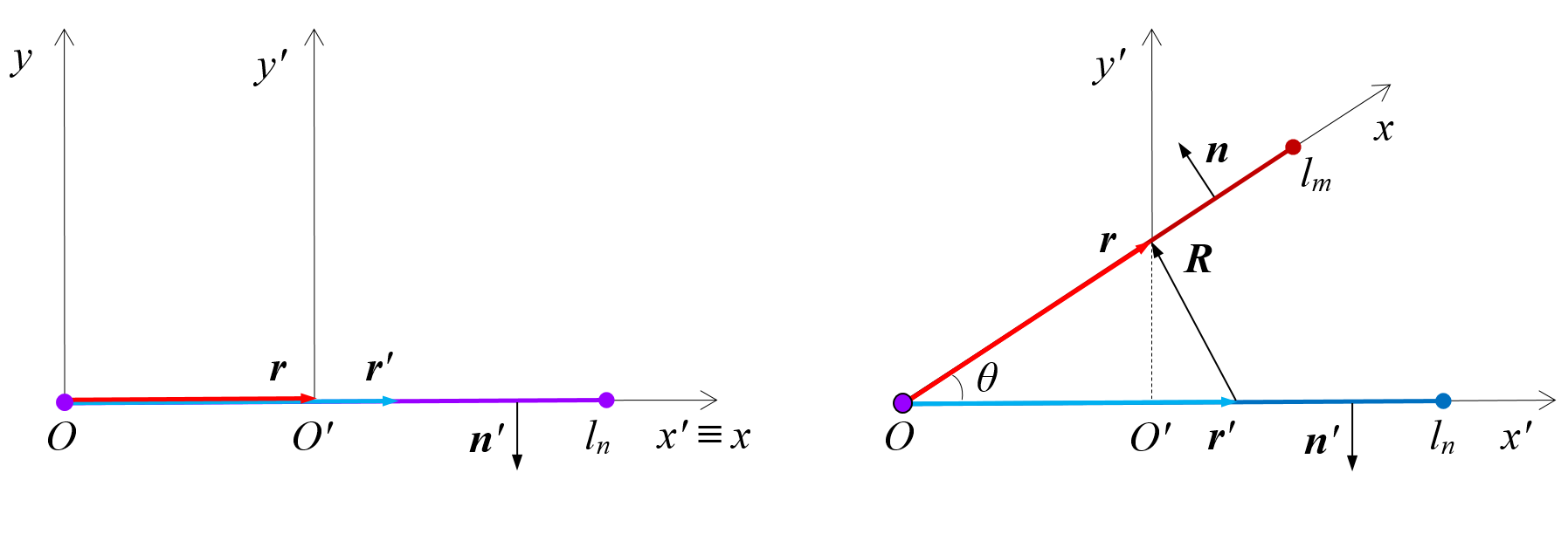
Figure 3: Sketches of the reference frames $Oxy$, $O^{\prime}x^{\prime}y^{\prime}$ relative to the coordinates $\mathbf{r}$ and $\mathbf{r}^{\prime}$ for the double integration over coincident (left) and adjacent (right) segments $S_{m}$ and $S_{n}$, respectively.

Making use of the following definitions:

$$I_{\alpha}^{n}\left(x\right) \equiv\fint_{-x}^{l_{n}-x}dx^{\prime}H_{0}^{(1,2)}\left(k\left|x^{\prime}\right|\right);$$ (25)

$$I_{\beta}^{n}\left(x\right) \equiv\frac{x}{l_{n}}\fint_{-x}^{l_{n}-x}dx^{\prime}H_{0}^{(1,2)}\left(k\left|x^{\prime}\right|\right);$$ (26)

$$I_{\gamma}^{n}\left(x\right) \equiv\fint_{-x}^{l_{n}-x}dx^{\prime}H_{0}^{(1,2)}\left(k\left|x^{\prime}\right|\right)\frac{\left(x^{\prime}+x\right)}{l_{n}};$$ (27)

$$I_{\delta}^{n}\left(x\right) \equiv\frac{x}{l_{n}}\fint_{-x}^{l_{n}-x}dx^{\prime}H_{0}^{(1,2)}\left(k\left|x^{\prime}\right|\right)\frac{\left(x^{\prime}+x\right)}{l_{n}},$$ (28)

the above integrals are rewritten as:

$$I_{11}^{n} =\frac{i}{4}\int_{0}^{l_{n}}dx\left[I_{\alpha}^{n}\left(x\right)-I_{\beta}^{n}\left(x\right)-I_{\gamma}^{n}\left(x\right)+I_{\delta}^{n}\left(x\right)\right];$$ (29)

$$I_{12}^{n} =\frac{i}{4}\int_{0}^{l_{n}}dx\left[I_{\gamma}^{n}\left(x\right)-I_{\delta}^{n}\left(x\right)\right];$$ (30)

$$I_{21}^{n} =\frac{i}{4}\int_{0}^{l_{n}}dx\left[I_{\beta}^{n}\left(x\right)-I_{\delta}^{n}\left(x\right)\right];$$ (31)

$$I_{22}^{n} =\frac{i}{4}\int_{0}^{l_{n}}dx\,I_{\delta}^{n}\left(x\right).$$ (32)

Let us focus on $I_{\alpha}^{n}\left(x\right)$:

$$I_{\alpha}^{n}\left(x\right) =\int_{-x}^{0}dx^{\prime}H_{0}^{(1,2)}\left(-kx^{\prime}\right)+\int_{0}^{l_{n}-x}dx^{\prime}H_{0}^{(1,2)}\left(kx^{\prime}\right)$$

$$=\frac{1}{k}\int_{0}^{kx}dx^{\prime}H_{0}^{(1,2)}\left(x^{\prime}\right)+\frac{1}{k}\int_{0}^{k\left(l_{n}-x\right)}dx^{\prime}H_{0}^{(1,2)}\left(x^{\prime}\right),$$ (33)

where the changes of variable $x^{\prime}\rightarrow-kx^{\prime}$ and $x^{\prime}\rightarrow kx^{\prime}$ have been employed to transform the first and second integrals, respectively. Now, applying the same strategy to (26)-(28) and introducing the useful definitions:

$$\mathcal{I}_{0}\left(\sigma\right) \equiv\int_{0}^{\sigma}dx^{\prime}H_{0}^{(1,2)}\left(x^{\prime}\right);$$ (34)

$$\mathcal{I}_{1}\left(\sigma\right) \equiv\int_{0}^{\sigma}dx^{\prime}H_{0}^{(1,2)}\left(x^{\prime}\right)\,x^{\prime},$$ (35)

we get:

$$I_{\alpha}^{n}\left(x\right) =\frac{1}{k}\left\{\mathcal{I}_{0}\left(kx\right)+\mathcal{I}_{0}\left[k\left(l_{n}-x\right)\right]\right\};$$ (36)

$$I_{\beta}^{n}\left(x\right) =\frac{x}{l_{n}}I_{\alpha}^{n}\left(x\right);$$ (37)

$$I_{\gamma}^{n}\left(x\right) =I_{\beta}^{n}\left(x\right)+\frac{1}{k^{2}l_{n}}\left\{\mathcal{I}_{1}\left[k\left(l_{n}-x\right)\right]-\mathcal{I}_{1}\left(kx\right)\right\};$$ (38)

$$I_{\delta}^{n}\left(x\right) =\frac{x}{l_{n}}I_{\gamma}^{n}\left(x\right).$$ (39)

In order to determine a closed-form expression for the integrals (34) and (35), reference is made to some tabulated formulas for Bessel functions of the first and second kind [9]:

$$\int_{0}^{1}ds\,J_{\nu}\left(\sigma s\right)s^{\nu} =2^{\nu-1}\sigma^{-\nu}\sqrt{\pi}\,\Gamma\left(\nu+\frac{1}{2}\right)\left[J_{\nu}\left(\sigma\right)\mathbf{H}_{\nu-1}\left(\sigma\right)-\mathbf{H}_{\nu}\left(\sigma\right)J_{\nu-1}\left(\sigma\right)\right];$$ (40)

$$\int_{0}^{1}ds\,Y_{\nu}\left(\sigma s\right)s^{\nu} =2^{\nu-1}\sigma^{-\nu}\sqrt{\pi}\,\Gamma\left(\nu+\frac{1}{2}\right)\left[Y_{\nu}\left(\sigma\right)\mathbf{H}_{\nu-1}\left(\sigma\right)-\mathbf{H}_{\nu}\left(\sigma\right)Y_{\nu-1}\left(\sigma\right)\right];$$ (41)

$$\int_{0}^{1}ds\,J_{\nu}\left(\sigma s\right)s^{\nu+1} =\sigma^{-1}J_{\nu+1}\left(\sigma\right);$$ (42)

$$\int_{0}^{1}ds\,Y_{\nu}\left(\sigma s\right)s^{\nu+1} =\sigma^{-1}Y_{\nu+1}\left(\sigma\right)+2^{\nu+1}\sigma^{-\nu-2}\pi^{-1}\Gamma\left(\nu+1\right),$$ (43)

where $\mathbf{H}_{\nu}$ represents the Struve function of order $\nu$ and $\Gamma$ is the Gamma function. If we combine the previous formulas using $H_{\nu}^{(1,2)}\equiv J_{\nu}\pm iY_{\nu}$, we obtain:

$$\int_{0}^{1}ds\,H_{\nu}^{(1,2)}\left(\sigma s\right)s^{\nu} =2^{\nu-1}\sigma^{-\nu}\sqrt{\pi}\,\Gamma\left(\nu+\frac{1}{2}\right)\left[H_{\nu}^{(1,2)}\left(\sigma\right)\mathbf{H}_{\nu-1}\left(\sigma\right)-H_{\nu-1}^{(1,2)}\left(\sigma\right)\mathbf{H}_{\nu}\left(\sigma\right)\right];$$ (44)

$$\int_{0}^{1}ds\,H_{\nu}^{(1,2)}\left(\sigma s\right)s^{\nu+1} =\sigma^{-1}H_{\nu+1}^{(1,2)}\left(\sigma\right)\pm i2^{\nu+1}\sigma^{-\nu-2}\pi^{-1}\Gamma\left(\nu+1\right),$$ (45)

which give us the sought results for $\nu=0$:

$$\mathcal{I}_{0}\left(\sigma\right) =\frac{\pi}{2}\sigma\left[H_{0}^{(1,2)}\left(\sigma\right)\mathbf{H}_{-1}\left(\sigma\right)+H_{1}^{(1,2)}\left(\sigma\right)\mathbf{H}_{0}\left(\sigma\right)\right];$$ (46)

$$\mathcal{I}_{1}\left(\sigma\right) =\sigma H_{1}^{(1,2)}\left(\sigma\right)\pm\frac{2}{\pi}i.$$ (47)

It is fundamental to note that both $\mathcal{I}_{0}\left(\sigma\right)$ and $\mathcal{I}_{1}\left(\sigma\right)$ are regular functions with removable singularity at $\sigma=0$, as displayed in Figure 4.

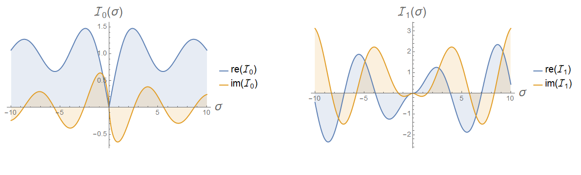
Figure 4: Plots of the functions $\mathcal{I}_{0}\left(\sigma\right)$ and $\mathcal{I}_{1}\left(\sigma\right)$ defined in (34) and (35) when only the first kind Hankel function $H_{0}^{(1)}\left(x^{\prime}\right)$ is considered.

That is to say, the remaining integrals in (29)-(32) are no longer singular and can be approximated with good accuracy by standard Gauss-Legendre quadrature formulas.

Let us now try to further simplify the resulting expressions.

$$\int_{0}^{l_{n}}dx\,I_{\alpha}^{n}\left(x\right) =\frac{1}{k}\int_{0}^{l_{n}}dx\,\mathcal{I}_{0}\left(kx\right)+\frac{1}{k}\int_{0}^{l_{n}}dx\,\mathcal{I}_{0}\left[k\left(l_{n}-x\right)\right]$$

$$=\frac{1}{k^{2}}\int_{0}^{kl_{n}}dx\,\mathcal{I}_{0}\left(x\right)-\frac{1}{k^{2}}\int_{kl_{n}}^{0}dx\,\mathcal{I}_{0}\left(x\right)=\frac{2}{k^{2}}\int_{0}^{kl_{n}}dx\,\mathcal{I}_{0}\left(x\right);$$ (48)

$$\int_{0}^{l_{n}}dx\,I_{\beta}^{n}\left(x\right) =\frac{1}{kl_{n}}\int_{0}^{l_{n}}dx\,x\mathcal{I}_{0}\left(kx\right)+\frac{1}{kl_{n}}\int_{0}^{l_{n}}dx\,x\mathcal{I}_{0}\left[k\left(l_{n}-x\right)\right]$$

$$=\frac{1}{k^{3}l_{n}}\int_{0}^{kl_{n}}dx\,x\mathcal{I}_{0}\left(x\right)+\frac{1}{k^{2}l_{n}}\int_{0}^{kl_{n}}dx\,\left(l_{n}-\frac{x}{k}\right)\mathcal{I}_{0}\left(x\right)=\frac{1}{k^{2}}\int_{0}^{kl_{n}}dx\,\mathcal{I}_{0}\left(x\right).$$ (49)

For the next integral, it is useful to note that:

$$\int_{0}^{l_{n}}dx\,\left\{\mathcal{I}_{1}\left[k\left(l_{n}-x\right)\right]-\mathcal{I}_{1}\left(kx\right)\right\} =\frac{1}{k}\int_{0}^{kl_{n}}dx\,\mathcal{I}_{1}\left(x\right)-\frac{1}{k}\int_{0}^{kl_{n}}dx\,\mathcal{I}_{1}\left(x\right)=0.$$ (50)

Therefore:

$$\int_{0}^{l_{n}}dx\,I_{\gamma}^{n}\left(x\right) =\int_{0}^{l_{n}}dx\,I_{\beta}^{n}\left(x\right)=\frac{1}{k^{2}}\int_{0}^{kl_{n}}dx\,\mathcal{I}_{0}\left(x\right).$$ (51)

The last integral can be arrived at by considering the followings:

$$\int_{0}^{l_{n}}dx\,\frac{x}{l_{n}}I_{\beta}^{n}\left(x\right) =\frac{1}{kl_{n}^{2}}\int_{0}^{l_{n}}dx\,x^{2}\mathcal{I}_{0}\left(kx\right)+\frac{1}{kl_{n}^{2}}\int_{0}^{l_{n}}dx\,x^{2}\mathcal{I}_{0}\left[k\left(l_{n}-x\right)\right]$$

$$=\frac{1}{k^{2}l_{n}^{2}}\int_{0}^{kl_{n}}dx\,\left[\frac{x^{2}}{k^{2}}\mathcal{I}_{0}\left(x\right)+\left(l_{n}-\frac{x}{k}\right)^{2}\mathcal{I}_{0}\left(x\right)\right]$$

$$=\frac{1}{k^{2}l_{n}^{2}}\int_{0}^{kl_{n}}dx\,\left(l_{n}^{2}-\frac{2l_{n}}{k}x+\frac{2}{k^{2}}x^{2}\right)\mathcal{I}_{0}\left(x\right);$$ (52)

$$\frac{1}{k^{2}l_{n}^{2}}\int_{0}^{l_{n}}dx\,\left\{x\mathcal{I}_{1}\left[k\left(l_{n}-x\right)\right]-x\mathcal{I}_{1}\left(kx\right)\right\}$$

$$=\frac{1}{k^{3}l_{n}^{2}}\int_{0}^{kl_{n}}dx\,\left[\left(l_{n}-\frac{x}{k}\right)\mathcal{I}_{1}\left(x\right)-\frac{x}{k}\mathcal{I}_{1}\left(x\right)\right]$$

$$=\frac{1}{k^{3}l_{n}^{2}}\int_{0}^{kl_{n}}dx\,\left(l_{n}-\frac{2}{k}x\right)\mathcal{I}_{1}\left(x\right).$$ (53)

As the careful reader may notice, integrations involving $\mathcal{I}_{1}\left(x\right)$ and $x\,\mathcal{I}_{1}\left(x\right)$ can still be evaluated analytically with the help of (44) and (45):

$$\int_{0}^{kl_{n}}dx\,\mathcal{I}_{1}\left(x\right) =\int_{0}^{kl_{n}}dx\,\left[xH_{1}^{(1,2)}\left(x\right)\pm\frac{2}{\pi}i\right]$$

$$=\frac{kl_{n}\pi}{2}\left[H_{1}^{(1,2)}\left(kl_{n}\right)\mathbf{H}_{0}\left(kl_{n}\right)-H_{0}^{(1,2)}\left(kl_{n}\right)\mathbf{H}_{1}\left(kl_{n}\right)\right]\pm\frac{2kl_{n}}{\pi}i;$$ (54)

$$\int_{0}^{kl_{n}}dx\,x\mathcal{I}_{1}\left(x\right)=\int_{0}^{kl_{n}}dx\,\left[x^{2}H_{1}^{(1,2)}\left(x\right)\pm\frac{2i}{\pi}x\right]=k^{2}l_{n}^{2}H_{2}^{(1,2)}\left(kl_{n}\right)\pm\frac{i}{\pi}\left(k^{2}l_{n}^{2}+4\right),$$ (55)

so that:

$$\int_{0}^{l_{n}}dx\,I_{\delta}^{n}\left(x\right) =\frac{1}{k^{2}l_{n}^{2}}\int_{0}^{kl_{n}}dx\,\left(l_{n}^{2}-\frac{2l_{n}}{k}x+\frac{2}{k^{2}}x^{2}\right)\mathcal{I}_{0}\left(x\right)+$$

$$+\frac{\pi}{2k^{2}}\left[H_{1}^{(1,2)}\left(kl_{n}\right)\mathbf{H}_{0}\left(kl_{n}\right)-H_{0}^{(1,2)}\left(kl_{n}\right)\mathbf{H}_{1}\left(kl_{n}\right)\right]-\frac{2}{k^{2}}H_{2}^{(1,2)}\left(kl_{n}\right)\mp\frac{8i}{\pi k^{4}l_{n}^{2}}.$$ (56)

Gathering together the results in (48), (49), (51) and (56), we are finally able to rewrite (29)-(32) as follows:

$$I_{11}^{n}=I_{22}^{n} =\frac{i\pi}{8k^{2}}\left[H_{1}^{(1,2)}\left(kl_{n}\right)\mathbf{H}_{0}\left(kl_{n}\right)-H_{0}^{(1,2)}\left(kl_{n}\right)\mathbf{H}_{1}\left(kl_{n}\right)\right]+$$

$$-\frac{i}{2k^{2}}H_{2}^{(1,2)}\left(kl_{n}\right)\pm\frac{2}{\pi k^{4}l_{n}^{2}}+\frac{i}{4k^{2}}\varGamma_{0}\left(kl_{n}\right)+\frac{i}{2k^{4}l_{n}^{2}}\varGamma_{2}\left(kl_{n}\right);$$ (57)

$$I_{12}^{n}=I_{21}^{n} =-I_{11}^{n}+\frac{i}{4k^{2}}\varGamma_{0}\left(kl_{n}\right),$$ (58)

where the remaining integrals:

$$\varGamma_{0}\left(\sigma\right) \equiv\int_{0}^{\sigma}dx\,\mathcal{I}_{0}\left(x\right)=\frac{\pi}{2}\int_{0}^{\sigma}dx\,x\left[H_{0}^{(1,2)}\left(x\right)\mathbf{H}_{-1}\left(x\right)+H_{1}^{(1,2)}\left(x\right)\mathbf{H}_{0}\left(x\right)\right];$$ (59)

$$\varGamma_{2}\left(\sigma\right) \equiv\int_{0}^{\sigma}dx\,\mathcal{I}_{0}\left(x\right)\,x\left(x-\sigma\right)=\frac{\pi}{2}\int_{0}^{\sigma}dx\,x^{2}\left(x-\sigma\right)\left[H_{0}^{(1,2)}\left(x\right)\mathbf{H}_{-1}\left(x\right)+H_{1}^{(1,2)}\left(x\right)\mathbf{H}_{0}\left(x\right)\right]$$ (60)

are left to Gauss-Legendre quadrature formulas.

To summarize, the singular double integrals (21)-(24) have been rewritten through (57) and (58) as a combination of the regular single integrals (59)-(60) and of some well-known analytic functions.

3.2 Integration over adjacent elements

Whenever the elements $S_{m}$ and $S_{n}$ in (7) are adjacent, the Green function (11) diverges in correspondence of the common vertex. As it is clear from Figure 2, this can happen when the $i$-th and $j$-th mesh nodes coincide as well as when they are first or second neighbors. In order to establish the strength of the singularity, the following expansion of the zeroth order Hankel function for small argument must be considered [8]:

$$H_{0}^{(1,2)}\left(z\right)\sim 1\pm\frac{2i}{\pi}\left(\log z+\gamma-\log 2\right),$$ (61)

where $\gamma$ is the Euler’s constant. It is important to note that the integrand in (7) is well-behaved when the product of the functions $p_{i}^{m}\left(\mathbf{r}\right)$ and $p_{j}^{n}\left(\mathbf{r}^{\prime}\right)$ is zero at the common vertex, since it cancels the singularity of the Green function. Standard Gauss-Legendre quadrature applies even when both $p_{i}^{m}\left(\mathbf{r}\right)$ and $p_{j}^{n}\left(\mathbf{r}^{\prime}\right)$ are one at the common vertex, i.e. for $i\equiv j$, as the logarithmic divergence is weak enough to be integrable and the singular end point is not considered. To improve the accuracy of the results, adaptive integration algorithms can be used in this case (see, for instance, [6]).

4 Double layer and adjoint double layer operators

4.1 Integration over coincident elements

When $S_{m}=S_{n}$, the double integrals appearing in (8) and (9) vanish identically, as follows from the fact that $\mathbf{R}\perp\mathbf{n}$ when both $\mathbf{r}$ and $\mathbf{r}^{\prime}$ lie on the same segment with unit normal $\mathbf{n}$.

4.2 Integration over adjacent elements

Making use of the following expansion of the first order Hankel function for small argument [8]:

$$H_{1}^{(1,2)}\left(z\right)\sim\mp\frac{2i}{\pi z},$$ (62)

it is easy to see that the only singular contribution to the integrations over adjacent segments in (8) and (9) is achieved, once again, when both $p_{i}^{m}\left(\mathbf{r}\right)$ and $p_{j}^{n}\left(\mathbf{r}^{\prime}\right)$ are one at the common vertex. In this case, however, the singularity is stronger than that in Section 3.2 and direct use of Gauss-Legendre quadrature formulas may lead to inaccurate results. In order to avoid this issue, a viable technique consists in introducing a coordinate transformation with vanishing Jacobian at the common vertex to cancel the singularity [3]. In A, this method is applied to the double layer integral; of course, the same procedure can be used in the adjoint double layer case with the appropriate changes.

5 Hypersingular operator: direct method

5.1 Integration over coincident elements

When $S_{m}=S_{n}$, the singular double integrals in (10) are of the form:

$$\frac{ik}{4}\int_{S_{n}}d\mathbf{r}\int_{S_{n}}d\mathbf{r}^{\prime}\frac{H_{1}^{(1,2)}\left(k\left|\mathbf{r}-\mathbf{r}^{\prime}\right|\right)}{\left|\mathbf{r}-\mathbf{r}^{\prime}\right|}p_{i}^{n}\left(\mathbf{r}\right)p_{j}^{n}\left(\mathbf{r}^{\prime}\right).$$ (63)

Adopting the same convention introduced in Section 3.1, we have:

$$\frac{ik}{4}\int_{0}^{l_{n}}dx\int_{-x}^{l_{n}-x}dx^{\prime}\frac{H_{1}^{(1,2)}\left(k\left|x^{\prime}\right|\right)}{\left|x^{\prime}\right|}p_{i}^{n}\left(x\right)\widetilde{p}_{j}^{n}\left(x^{\prime},x\right).$$ (64)

Making use of the recurrence relations for Hankel functions [9]:

$$zH_{\nu-1}^{(1,2)}\left(z\right)+zH_{\nu+1}^{(1,2)}\left(z\right) =2\nu H_{\nu}^{(1,2)}\left(z\right);$$ (65)

$$H_{\nu-1}^{(1,2)}\left(z\right)-H_{\nu+1}^{(1,2)}\left(z\right) =2\frac{d}{dz}H_{\nu}^{(1,2)}\left(z\right)\equiv 2\dot{H}_{\nu}^{(1,2)}\left(z\right),$$ (66)

we get:

$$\frac{ik^{2}}{4}\int_{0}^{l_{n}}dx\int_{-x}^{l_{n}-x}dx^{\prime}\left[H_{0}^{(1,2)}\left(k\left|x^{\prime}\right|\right)-\dot{H}_{1}^{(1,2)}\left(k\left|x^{\prime}\right|\right)\right]p_{i}^{n}\left(x\right)\widetilde{p}_{j}^{n}\left(x^{\prime},x\right).$$ (67)

This last equation, together with (19), (20) and (21)-(24), gives rise to four expressions:

$$\varUpsilon_{11}^{n} \equiv k^{2}I_{11}^{n}-\frac{ik^{2}}{4}\int_{0}^{l_{n}}dx\int_{-x}^{l_{n}-x}dx^{\prime}\dot{H}_{1}^{(1,2)}\left(k\left|x^{\prime}\right|\right)\left(1-\frac{x}{l_{n}}\right)\left[1-\frac{\left(x^{\prime}+x\right)}{l_{n}}\right];$$ (68)

$$\varUpsilon_{12}^{n} \equiv k^{2}I_{12}^{n}-\frac{ik^{2}}{4}\int_{0}^{l_{n}}dx\int_{-x}^{l_{n}-x}dx^{\prime}\dot{H}_{1}^{(1,2)}\left(k\left|x^{\prime}\right|\right)\left(1-\frac{x}{l_{n}}\right)\left[\frac{\left(x^{\prime}+x\right)}{l_{n}}\right];$$ (69)

$$\varUpsilon_{21}^{n} \equiv k^{2}I_{21}^{n}-\frac{ik^{2}}{4}\int_{0}^{l_{n}}dx\int_{-x}^{l_{n}-x}dx^{\prime}\dot{H}_{1}^{(1,2)}\left(k\left|x^{\prime}\right|\right)\left(\frac{x}{l_{n}}\right)\left[1-\frac{\left(x^{\prime}+x\right)}{l_{n}}\right];$$ (70)

$$\varUpsilon_{22}^{n} \equiv k^{2}I_{22}^{n}-\frac{ik^{2}}{4}\int_{0}^{l_{n}}dx\int_{-x}^{l_{n}-x}dx^{\prime}\dot{H}_{1}^{(1,2)}\left(k\left|x^{\prime}\right|\right)\left(\frac{x}{l_{n}}\right)\left[\frac{\left(x^{\prime}+x\right)}{l_{n}}\right],$$ (71)

which can be recast in the following form:

$$\varUpsilon_{11}^{n} =k^{2}I_{11}^{n}-\frac{ik^{2}}{4}\int_{0}^{l_{n}}dx\left[\varUpsilon_{\alpha}^{n}\left(x\right)-\varUpsilon_{\beta}^{n}\left(x\right)-\varUpsilon_{\gamma}^{n}\left(x\right)+\varUpsilon_{\delta}^{n}\left(x\right)\right];$$ (72)

$$\varUpsilon_{12}^{n} =k^{2}I_{12}^{n}-\frac{ik^{2}}{4}\int_{0}^{l_{n}}dx\left[\varUpsilon_{\gamma}^{n}\left(x\right)-\varUpsilon_{\delta}^{n}\left(x\right)\right];$$ (73)

$$\varUpsilon_{21}^{n} =k^{2}I_{12}^{n}-\frac{ik^{2}}{4}\int_{0}^{l_{n}}dx\left[\varUpsilon_{\beta}^{n}\left(x\right)-\varUpsilon_{\delta}^{n}\left(x\right)\right];$$ (74)

$$\varUpsilon_{22}^{n} =k^{2}I_{11}^{n}-\frac{ik^{2}}{4}\int_{0}^{l_{n}}dx\,\varUpsilon_{\delta}^{n}\left(x\right),$$ (75)

where (57), (58) have been used and:

$$\varUpsilon_{\alpha}^{n}\left(x\right) \equiv\int_{-x}^{l_{n}-x}dx^{\prime}\dot{H}_{1}^{(1,2)}\left(k\left|x^{\prime}\right|\right);$$ (76)

$$\varUpsilon_{\beta}^{n}\left(x\right) \equiv\frac{x}{l_{n}}\int_{-x}^{l_{n}-x}dx^{\prime}\dot{H}_{1}^{(1,2)}\left(k\left|x^{\prime}\right|\right);$$ (77)

$$\varUpsilon_{\gamma}^{n}\left(x\right) \equiv\int_{-x}^{l_{n}-x}dx^{\prime}\dot{H}_{1}^{(1,2)}\left(k\left|x^{\prime}\right|\right)\frac{\left(x^{\prime}+x\right)}{l_{n}};$$ (78)

$$\varUpsilon_{\delta}^{n}\left(x\right) \equiv\frac{x}{l_{n}}\int_{-x}^{l_{n}-x}dx^{\prime}\dot{H}_{1}^{(1,2)}\left(k\left|x^{\prime}\right|\right)\frac{\left(x^{\prime}+x\right)}{l_{n}}.$$ (79)

As in Section 3.1, these integrals will be split in order to get rid of absolute values. For instance:

$$\varUpsilon_{\alpha}^{n}\left(x\right) =\int_{-x}^{0}dx^{\prime}\dot{H}_{1}^{(1,2)}\left(-kx^{\prime}\right)+\int_{0}^{l_{n}-x}dx^{\prime}\dot{H}_{1}^{(1,2)}\left(kx^{\prime}\right)$$

$$=\frac{1}{k}\int_{0}^{kx}dx^{\prime}\dot{H}_{1}^{(1,2)}\left(x^{\prime}\right)+\frac{1}{k}\int_{0}^{k\left(l_{n}-x\right)}dx^{\prime}\dot{H}_{1}^{(1,2)}\left(x^{\prime}\right)$$ (80)

and similarly for the other three integrals. Then, we define:

$$\varUpsilon_{0}\left(\sigma\right) \equiv\int_{0}^{\sigma}dx^{\prime}\dot{H}_{1}^{(1,2)}\left(x^{\prime}\right);$$ (81)

$$\varUpsilon_{1}\left(\sigma\right) \equiv\int_{0}^{\sigma}dx^{\prime}\dot{H}_{1}^{(1,2)}\left(x^{\prime}\right)\,x^{\prime},$$ (82)

so that:

$$\varUpsilon_{\alpha}^{n}\left(x\right) =\frac{1}{k}\left\{\varUpsilon_{0}\left(kx\right)+\varUpsilon_{0}\left[k\left(l_{n}-x\right)\right]\right\};$$ (83)

$$\varUpsilon_{\beta}^{n}\left(x\right) =\frac{x}{l_{n}}\varUpsilon_{\alpha}^{n}\left(x\right);$$ (84)

$$\varUpsilon_{\gamma}^{n}\left(x\right) =\varUpsilon_{\beta}^{n}\left(x\right)+\frac{1}{k^{2}l_{n}}\left\{\varUpsilon_{1}\left[k\left(l_{n}-x\right)\right]-\varUpsilon_{1}\left(kx\right)\right\};$$ (85)

$$\varUpsilon_{\delta}^{n}\left(x\right) =\frac{x}{l_{n}}\varUpsilon_{\gamma}^{n}\left(x\right).$$ (86)

Unfortunately, both (81) and (82) are singular. A regularization for $\varUpsilon_{0}\left(\sigma\right)$ can be achieved by analytic continuation:

$$\varUpsilon_{0}\left(\sigma\right) =\frac{1}{2}\lim_{\varepsilon\rightarrow 0}\left[\int_{0}^{\sigma}dx^{\prime}\dot{H}_{1}^{(1,2)}\left(x^{\prime}-i\varepsilon\right)+\int_{0}^{\sigma}dx^{\prime}\dot{H}_{1}^{(1,2)}\left(x^{\prime}+i\varepsilon\right)\right]$$

$$=\frac{1}{2}\lim_{\varepsilon\rightarrow 0}\left[\int_{-i\varepsilon}^{\sigma-i\varepsilon}dx^{\prime}\dot{H}_{1}^{(1,2)}\left(x^{\prime}\right)+\int_{i\varepsilon}^{\sigma+i\varepsilon}dx^{\prime}\dot{H}_{1}^{(1,2)}\left(x^{\prime}\right)\right]$$

$$=\frac{1}{2}\lim_{\varepsilon\rightarrow 0}\left[H_{1}^{(1,2)}\left(\sigma-i\varepsilon\right)-H_{1}^{(1,2)}\left(-i\varepsilon\right)+H_{1}^{(1,2)}\left(\sigma+i\varepsilon\right)-H_{1}^{(1,2)}\left(i\varepsilon\right)\right]$$

$$=H_{1}^{(1,2)}\left(\sigma\right)-\frac{1}{2}\lim_{\varepsilon\rightarrow 0}\left[H_{1}^{(1,2)}\left(i\varepsilon\right)+H_{1}^{(1,2)}\left(-i\varepsilon\right)\right]=H_{1}^{(1,2)}\left(\sigma\right),$$ (87)

where the expansion (62) has been employed in the last step. Now, exploiting the fact that the divergent integral (82) only appears through the difference $\varUpsilon_{1}\left[k\left(l_{n}-x\right)\right]-\varUpsilon_{1}\left(kx\right)$, let:

$$\delta\varUpsilon_{1}\left(\sigma_{a},\sigma_{b}\right) \equiv\varUpsilon_{1}\left(\sigma_{b}\right)-\varUpsilon_{1}\left(\sigma_{a}\right)=\fint_{\sigma_{a}}^{\sigma_{b}}dx^{\prime}\dot{H}_{1}^{(1,2)}\left(x^{\prime}\right)\,x^{\prime}$$

$$=\lim_{\varepsilon\rightarrow 0}\left[\int_{\varepsilon}^{\sigma_{b}}dx^{\prime}\dot{H}_{1}^{(1,2)}\left(x^{\prime}\right)\,x^{\prime}-\int_{\varepsilon}^{\sigma_{a}}dx^{\prime}\dot{H}_{1}^{(1,2)}\left(x^{\prime}\right)\,x^{\prime}\right].$$ (88)

Each of the two terms in the last expression can be integrated by parts:

$$\int_{\varepsilon}^{\sigma}dx^{\prime}\dot{H}_{1}^{(1,2)}\left(x^{\prime}\right)\,x^{\prime} =\sigma H_{1}^{(1,2)}\left(\sigma\right)-\varepsilon H_{1}^{(1,2)}\left(\varepsilon\right)-\int_{\varepsilon}^{\sigma}dx^{\prime}H_{1}^{(1,2)}\left(x^{\prime}\right)$$ (89)

where, using (66):

$$\int_{\varepsilon}^{\sigma}dx^{\prime}H_{1}^{(1,2)}\left(x^{\prime}\right) =-\int_{\varepsilon}^{\sigma}dx^{\prime}\dot{H}_{0}^{(1,2)}\left(x^{\prime}\right)=-\left[H_{0}^{(1,2)}\left(\sigma\right)-H_{0}^{(1,2)}\left(\varepsilon\right)\right].$$ (90)

Then, taking the difference:

$$\delta\varUpsilon_{1}\left(\sigma_{a},\sigma_{b}\right) =\sigma_{b}H_{1}^{(1,2)}\left(\sigma_{b}\right)-\sigma_{a}H_{1}^{(1,2)}\left(\sigma_{a}\right)+H_{0}^{(1,2)}\left(\sigma_{b}\right)-H_{0}^{(1,2)}\left(\sigma_{a}\right).$$ (91)

Let us apply the above results to simplify expressions (83)-(86):

$$\varUpsilon_{\alpha}^{n}\left(x\right) =\frac{1}{k}\left\{H_{1}^{(1,2)}\left(kx\right)+H_{1}^{(1,2)}\left[k\left(l_{n}-x\right)\right]\right\};$$ (92)

$$\varUpsilon_{\beta}^{n}\left(x\right) =\frac{x}{l_{n}}\varUpsilon_{\alpha}^{n}\left(x\right);$$ (93)

$$\varUpsilon_{\gamma}^{n}\left(x\right) =\varUpsilon_{\beta}^{n}\left(x\right)+\frac{1}{k^{2}l_{n}}\left\{k\left(l_{n}-x\right)H_{1}^{(1,2)}\left[k\left(l_{n}-x\right)\right]-kxH_{1}^{(1,2)}\left(kx\right)+\right.$$ (94)

$$\left.+H_{0}^{(1,2)}\left[k\left(l_{n}-x\right)\right]-H_{0}^{(1,2)}\left(kx\right)\right\};$$ (95)

$$\varUpsilon_{\delta}^{n}\left(x\right) =\frac{x}{l_{n}}\varUpsilon_{\gamma}^{n}\left(x\right).$$ (96)

In order to be able to rewrite (72)-(75) in closed form, the previous equations will be integrated analytically between $\varepsilon$ and $l_{n}-\varepsilon$ and the limit $\varepsilon\rightarrow 0$ will be taken explicitly whenever possible, otherwise implicitly assumed. Starting with $\varUpsilon_{\alpha}^{n}\left(x\right)$, making use of the changes of variable $x\rightarrow kx$, $x\rightarrow k\left(l_{n}-x\right)$ and of formula (90), we have:

$$\int_{\varepsilon}^{l_{n}-\varepsilon}dx\,\varUpsilon_{\alpha}^{n}\left(x\right) =\frac{1}{k}\int_{\varepsilon}^{l_{n}-\varepsilon}dx\,\left\{H_{1}^{(1,2)}\left(kx\right)+H_{1}^{(1,2)}\left[k\left(l_{n}-x\right)\right]\right\}$$

$$=\frac{1}{k^{2}}\int_{k\varepsilon}^{kl_{n}}dx\,H_{1}^{(1,2)}\left(x\right)-\frac{1}{k^{2}}\int_{kl_{n}}^{k\varepsilon}dx\,H_{1}^{(1,2)}\left(x\right)$$

$$=\frac{2}{k^{2}}\int_{k\varepsilon}^{kl_{n}}dx\,H_{1}^{(1,2)}\left(x\right)=\frac{2}{k^{2}}\left[H_{0}^{(1,2)}\left(k\varepsilon\right)-H_{0}^{(1,2)}\left(kl_{n}\right)\right].$$ (97)

The integral of $\varUpsilon_{\beta}^{n}\left(x\right)$ is treated analogously:

$$\int_{\varepsilon}^{l_{n}-\varepsilon}dx\,\varUpsilon_{\beta}^{n}\left(x\right) =\frac{1}{kl_{n}}\int_{\varepsilon}^{l_{n}-\varepsilon}dx\,\left\{xH_{1}^{(1,2)}\left(kx\right)+xH_{1}^{(1,2)}\left[k\left(l_{n}-x\right)\right]\right\}$$

$$=\frac{1}{k^{3}l_{n}}\int_{k\varepsilon}^{kl_{n}}dx\,xH_{1}^{(1,2)}\left(x\right)-\frac{1}{k^{2}l_{n}}\int_{kl_{n}}^{k\varepsilon}dx\,\left(l_{n}-\frac{x}{k}\right)H_{1}^{(1,2)}\left(x\right)$$

$$=\frac{1}{k^{3}l_{n}}\int_{k\varepsilon}^{kl_{n}}dx\,xH_{1}^{(1,2)}\left(x\right)+\frac{1}{k^{2}}\int_{k\varepsilon}^{kl_{n}}dx\,H_{1}^{(1,2)}\left(x\right)-\frac{1}{k^{3}l_{n}}\int_{k\varepsilon}^{kl_{n}}dx\,xH_{1}^{(1,2)}\left(x\right)$$

$$=\frac{1}{k^{2}}\int_{k\varepsilon}^{kl_{n}}dx\,H_{1}^{(1,2)}\left(x\right)=\frac{1}{k^{2}}\left[H_{0}^{(1,2)}\left(k\varepsilon\right)-H_{0}^{(1,2)}\left(kl_{n}\right)\right].$$ (98)

To compute the integral of $\varUpsilon_{\gamma}^{n}\left(x\right)$, we notice that:

$$\frac{1}{k^{2}l_{n}}\int_{\varepsilon}^{l_{n}-\varepsilon}dx\,\left\{k\left(l_{n}-x\right)H_{1}^{(1,2)}\left[k\left(l_{n}-x\right)\right]-kxH_{1}^{(1,2)}\left(kx\right)\right\}$$

$$=\frac{1}{k^{3}l_{n}}\left[\int_{k\varepsilon}^{kl_{n}}dx\,xH_{1}^{(1,2)}\left(x\right)-\int_{k\varepsilon}^{kl_{n}}dx\,xH_{1}^{(1,2)}\left(x\right)\right]=0$$ (99)

and similarly:

$$\frac{1}{k^{2}l_{n}}\int_{\varepsilon}^{l_{n}-\varepsilon}dx\,\left\{H_{0}^{(1,2)}\left[k\left(l_{n}-x\right)\right]-H_{0}^{(1,2)}\left(kx\right)\right\}$$

$$=\frac{1}{k^{3}l_{n}}\left[\int_{k\varepsilon}^{kl_{n}}dx\,H_{0}^{(1,2)}\left(x\right)-\int_{k\varepsilon}^{kl_{n}}dx\,H_{0}^{(1,2)}\left(x\right)\right]=0.$$ (100)

Therefore:

$$\int_{\varepsilon}^{l_{n}-\varepsilon}dx\,\varUpsilon_{\gamma}^{n}\left(x\right)=\int_{\varepsilon}^{l_{n}-\varepsilon}dx\,\varUpsilon_{\beta}^{n}\left(x\right)=\frac{1}{k^{2}}\left[H_{0}^{(1,2)}\left(k\varepsilon\right)-H_{0}^{(1,2)}\left(kl_{n}\right)\right].$$ (101)

The following results prove useful for the evaluation of the last integral:

$$\int_{\varepsilon}^{l_{n}-\varepsilon}dx\,\frac{x}{l_{n}}\varUpsilon_{\beta}^{n}\left(x\right) =\frac{1}{kl_{n}^{2}}\int_{\varepsilon}^{l_{n}-\varepsilon}dx\,\left\{x^{2}H_{1}^{(1,2)}\left(kx\right)+x^{2}H_{1}^{(1,2)}\left[k\left(l_{n}-x\right)\right]\right\}$$

$$=\frac{1}{k^{2}l_{n}^{2}}\int_{k\varepsilon}^{kl_{n}}dx\,\left[\frac{x^{2}}{k^{2}}H_{1}^{(1,2)}\left(x\right)+\left(l_{n}-\frac{x}{k}\right)^{2}H_{1}^{(1,2)}\left(x\right)\right]$$

$$=\frac{1}{k^{2}l_{n}^{2}}\int_{k\varepsilon}^{kl_{n}}dx\,\left(l_{n}^{2}-\frac{2l_{n}}{k}x+\frac{2}{k^{2}}x^{2}\right)H_{1}^{(1,2)}\left(x\right);$$ (102)

$$\frac{1}{k^{2}l_{n}^{2}}\int_{\varepsilon}^{l_{n}-\varepsilon}dx\,\left\{k\left(l_{n}-x\right)xH_{1}^{(1,2)}\left[k\left(l_{n}-x\right)\right]-kx^{2}H_{1}^{(1,2)}\left(kx\right)\right\}$$

$$=\frac{1}{k^{3}l_{n}^{2}}\int_{k\varepsilon}^{kl_{n}}dx\,\left[x\left(l_{n}-\frac{x}{k}\right)H_{1}^{(1,2)}\left(x\right)-\frac{x^{2}}{k}H_{1}^{(1,2)}\left(x\right)\right]$$

$$=\frac{1}{k^{2}l_{n}^{2}}\int_{k\varepsilon}^{kl_{n}}dx\,\left(\frac{l_{n}}{k}x-\frac{2}{k^{2}}x^{2}\right)H_{1}^{(1,2)}\left(x\right);$$ (103)

$$\frac{1}{k^{2}l_{n}^{2}}\int_{\varepsilon}^{l_{n}-\varepsilon}dx\,\left\{xH_{0}^{(1,2)}\left[k\left(l_{n}-x\right)\right]-xH_{0}^{(1,2)}\left(kx\right)\right\}$$

$$=\frac{1}{k^{3}l_{n}^{2}}\int_{k\varepsilon}^{kl_{n}}dx\,\left[\left(l_{n}-\frac{x}{k}\right)H_{0}^{(1,2)}\left(x\right)-\frac{x}{k}H_{0}^{(1,2)}\left(x\right)\right]$$

$$=\frac{1}{k^{3}l_{n}}\int_{k\varepsilon}^{kl_{n}}dx\,H_{0}^{(1,2)}\left(x\right)-\frac{2}{k^{4}l_{n}^{2}}\int_{k\varepsilon}^{kl_{n}}dx\,xH_{0}^{(1,2)}\left(x\right)$$

$$=\frac{1}{k^{3}l_{n}}\mathcal{I}_{0}\left(kl_{n}\right)-\frac{2}{k^{4}l_{n}^{2}}\mathcal{I}_{1}\left(kl_{n}\right),$$ (104)

where (34) and (35) have been employed in the last step. Combining the previous expressions, we obtain:

$$\int_{\varepsilon}^{l_{n}-\varepsilon}dx\,\varUpsilon_{\delta}^{n}\left(x\right) =\frac{1}{k^{2}l_{n}^{2}}\int_{k\varepsilon}^{kl_{n}}dx\,\left(l_{n}^{2}-\frac{l_{n}}{k}x\right)H_{1}^{(1,2)}\left(x\right)+\frac{1}{k^{3}l_{n}}\mathcal{I}_{0}\left(kl_{n}\right)-\frac{2}{k^{4}l_{n}^{2}}\mathcal{I}_{1}\left(kl_{n}\right)$$

$$=\frac{1}{k^{2}}\int_{k\varepsilon}^{kl_{n}}dx\,H_{1}^{(1,2)}\left(x\right)-\frac{1}{k^{3}l_{n}}\int_{k\varepsilon}^{kl_{n}}dx\,xH_{1}^{(1,2)}\left(x\right)+\frac{1}{k^{3}l_{n}}\mathcal{I}_{0}\left(kl_{n}\right)-\frac{2}{k^{4}l_{n}^{2}}\mathcal{I}_{1}\left(kl_{n}\right),$$ (105)

which can be simplified using (90), the following formula:

$$\int_{0}^{\sigma}dx\,H_{1}^{(1,2)}\left(x\right)\,x =\frac{\pi\sigma}{2}\left[H_{1}^{(1,2)}\left(\sigma\right)\mathbf{H}_{0}\left(\sigma\right)-H_{0}^{(1,2)}\left(\sigma\right)\mathbf{H}_{1}\left(\sigma\right)\right],$$ (106)

derived from (44) with $\nu=1$, and equations (46) and (47):

$$\int_{\varepsilon}^{l_{n}-\varepsilon}dx\,\varUpsilon_{\delta}^{n}\left(x\right) =\frac{1}{k^{2}}\left[H_{0}^{(1,2)}\left(k\varepsilon\right)-H_{0}^{(1,2)}\left(kl_{n}\right)\right]+$$

$$+\frac{\pi}{2k^{2}}\left[H_{0}^{(1,2)}\left(kl_{n}\right)\mathbf{H}_{1}\left(kl_{n}\right)-H_{1}^{(1,2)}\left(kl_{n}\right)\mathbf{H}_{0}\left(kl_{n}\right)\right]+$$

$$+\frac{\pi}{2k^{2}}\left[H_{0}^{(1,2)}\left(kl_{n}\right)\mathbf{H}_{-1}\left(kl_{n}\right)+H_{1}^{(1,2)}\left(kl_{n}\right)\mathbf{H}_{0}\left(kl_{n}\right)\right]+$$

$$-\frac{2}{k^{4}l_{n}^{2}}\left[kl_{n}H_{1}^{(1,2)}\left(kl_{n}\right)\pm\frac{2}{\pi}i\right].$$ (107)

Finally, by the recurrence relations for Struve functions [9]:

$$\mathbf{H}_{\nu-1}\left(z\right) +\mathbf{H}_{\nu+1}\left(z\right)=\frac{2\nu}{z}\mathbf{H}_{\nu}\left(z\right)+\frac{1}{\sqrt{\pi}}\left(\frac{z}{2}\right)^{\nu}\frac{1}{\Gamma\left(\nu+\frac{3}{2}\right)},$$ (108)

we get:

$$\int_{\varepsilon}^{l_{n}-\varepsilon}dx\,\varUpsilon_{\delta}^{n}\left(x\right) =\frac{1}{k^{2}}H_{0}^{(1,2)}\left(k\varepsilon\right)-\frac{2}{k^{4}l_{n}^{2}}\left[kl_{n}H_{1}^{(1,2)}\left(kl_{n}\right)\pm\frac{2}{\pi}i\right].$$ (109)

Replacing (97), (98), (101) and (109) into equations (72)-(75) leads to:

$$\varUpsilon_{11}^{n} =\varUpsilon_{22}^{n}=k^{2}I_{11}^{n}-\frac{i}{4}H_{0}^{(1,2)}\left(k\varepsilon\right)+\frac{i}{2kl_{n}}H_{1}^{(1,2)}\left(kl_{n}\right)\mp\frac{1}{\pi k^{2}l_{n}^{2}};$$ (110)

$$\varUpsilon_{12}^{n} =\varUpsilon_{21}^{n}=k^{2}I_{12}^{n}+\frac{i}{4}H_{0}^{(1,2)}\left(kl_{n}\right)-\frac{i}{2kl_{n}}H_{1}^{(1,2)}\left(kl_{n}\right)\pm\frac{1}{\pi k^{2}l_{n}^{2}},$$ (111)

where $I_{11}^{n}$ and $I_{12}^{n}$ are given by (57) and (58), respectively, and the limit $\varepsilon\rightarrow 0$ is assumed. Owing to the logarithmic divergence of the function $H_{0}^{(1,2)}\left(k\varepsilon\right)$, both $\varUpsilon_{11}^{n}$ and $\varUpsilon_{22}^{n}$ are singular. In order for the matrix elements $N_{ii}$ in (10) to be well-defined, these singularities as well as those arising from the integration over adjacent segments must cancel in the sum over $\left\{m\in i\right\}\times\left\{n\in i\right\}$ (left column of Figure 2). This fundamental condition is checked in the next subsection. By explicitly removing the divergent term, equation (110) becomes:

$$\varUpsilon_{11}^{n}\mp\frac{1}{2\pi}\log\varepsilon =k^{2}I_{11}^{n}+\frac{i}{2kl_{n}}H_{1}^{(1,2)}\left(kl_{n}\right)-\frac{i}{4}\pm\frac{1}{2\pi}\left(\gamma+\log\frac{k}{2}-\frac{2}{k^{2}l_{n}^{2}}\right),$$ (112)

where (61) has been used.

5.2 Integration over adjacent elements

Let us consider the following expansions for small $z$ [8]:

$$\frac{H_{1}^{(1,2)}\left(z\right)}{z} \sim\frac{1}{2}\mp\frac{2i}{\pi}\frac{1}{z^{2}}\pm\frac{i}{\pi}\left(\log z-\frac{1}{2}+\gamma-\log 2\right);$$ (113)

$$H_{2}^{(1,2)}\left(z\right) \sim\mp\frac{i}{\pi}\mp\frac{4i}{\pi}\frac{1}{z^{2}}.$$ (114)

When only one of the two functions $p_{i}^{m}\left(\mathbf{r}\right)$ and $p_{j}^{n}\left(\mathbf{r}^{\prime}\right)$ equals unity at the common vertex, the integrations over adjacent segments in (10) can be treated via singularity cancellation as it is done in A for the double layer case. Whereas the logarithmic term does not constitute an issue, as explained in Section 3.2, it is apparent that a non-integrable singularity of the form $\sim R^{-2}$ arises when both basis functions are one at the common vertex. Once properly isolated, such divergent term proves to be equal and opposite to that appearing in (110), as it is shown below.

With reference to (113) and (114), a regularized version of the first and second order Hankel functions can be defined by singularity subtraction:

$$\widetilde{H}_{1}^{(1,2)}\left(z\right) \equiv H_{1}^{(1,2)}\left(z\right)\pm\frac{2i}{\pi}\frac{1}{z};$$ (115)

$$\widetilde{H}_{2}^{(1,2)}\left(z\right) \equiv H_{2}^{(1,2)}\left(z\right)\pm\frac{4i}{\pi}\frac{1}{z^{2}}.$$ (116)

This allows us to rewrite the divergent adjacent integrations in (10) as the sum of a regular part and a singular part:

$$\int_{S_{m}}d\mathbf{r}\int_{S_{n}}d\mathbf{r}^{\prime}\frac{\partial^{2}g\left(\mathbf{r},\mathbf{r}^{\prime}\right)}{\partial n\partial n^{\prime}}p_{i}^{m}\left(\mathbf{r}\right)p_{j}^{n}\left(\mathbf{r}^{\prime}\right)=\varUpsilon_{reg}^{m,n}+\varUpsilon_{sing}^{m,n},$$ (117)

where:

$$\varUpsilon_{reg}^{m,n} =\frac{ik^{2}}{4}\int_{S_{m}}d\mathbf{r}\int_{S_{n}}d\mathbf{r}^{\prime}\left[\frac{\widetilde{H}_{1}^{(1,2)}\left(kR\right)}{kR}\left(\mathbf{n}\cdot\mathbf{n}^{\prime}\right)-\widetilde{H}_{2}^{(1,2)}\left(kR\right)\frac{\left(\mathbf{R}\cdot\mathbf{n}\right)\left(\mathbf{R}\cdot\mathbf{n}^{\prime}\right)}{R^{2}}\right]p_{i}^{m}\left(\mathbf{r}\right)p_{j}^{n}\left(\mathbf{r}^{\prime}\right);$$ (118)

$$\varUpsilon_{sing}^{m,n} =\pm\frac{1}{2\pi}\int_{S_{m}}d\mathbf{r}\int_{S_{n}}d\mathbf{r}^{\prime}\left[\frac{\left(\mathbf{n}\cdot\mathbf{n}^{\prime}\right)}{R^{2}}-2\frac{\left(\mathbf{R}\cdot\mathbf{n}\right)\left(\mathbf{R}\cdot\mathbf{n}^{\prime}\right)}{R^{4}}\right]p_{i}^{m}\left(\mathbf{r}\right)p_{j}^{n}\left(\mathbf{r}^{\prime}\right)$$ (119)

and basis functions that equal one at the common vertex are assumed. The regular integral $\varUpsilon_{reg}^{m,n}$ is left to Gauss-Legendre quadrature formulas. Conversely, by fixing the reference frames $O^{\prime}x^{\prime}y^{\prime}$, $Oxy$ as in Figure 3 (right side), so that the basis functions are given by:

$$p_{i}^{m}\left(x\right)\equiv\begin{cases}1-\frac{x}{l_{m}}&\mathrm{if}\>x_{i}=0;\\ \frac{x}{l_{m}}&\mathrm{if}\>x_{i}=l_{m},\end{cases}$$ (120)

$$p_{j}^{n}\left(x^{\prime},x\right)\equiv\begin{cases}1-\frac{\left(x^{\prime}+x\cos\theta\right)}{l_{n}}&\mathrm{if}\>x_{j}^{\prime}=-x\cos\theta;\\ \frac{\left(x^{\prime}+x\cos\theta\right)}{l_{n}}&\mathrm{if}\>x_{j}^{\prime}=l_{n}-x\cos\theta,\end{cases}$$ (121)

the singular integral (119) leads back to:

$$\varUpsilon_{sing}^{m,n} =\mp\frac{1}{2\pi}\int_{0}^{l_{m}}dx\int_{-x\cos\theta}^{l_{n}-x\cos\theta}dx^{\prime}\left[\frac{\cos\theta}{x^{\prime 2}+x^{2}\sin^{2}\theta}-\frac{2x\sin^{2}\theta\left(x^{\prime}+x\cos\theta\right)}{\left(x^{\prime 2}+x^{2}\sin^{2}\theta\right)^{2}}\right]$$

$$\times\left(1-\frac{x}{l_{m}}\right)\left[1-\frac{\left(x^{\prime}+x\cos\theta\right)}{l_{n}}\right].$$ (122)

To carry out the inner integration, the following indefinite integrals come in handy [9]:

$$\int\frac{dx^{\prime}}{\left(x^{\prime 2}+a^{2}\right)^{2}} =\frac{1}{2a^{3}}\left[\frac{ax^{\prime}}{x^{\prime 2}+a^{2}}+\arctan\left(\frac{x^{\prime}}{a}\right)\right];$$ (123)

$$\int\frac{x^{\prime}dx^{\prime}}{\left(x^{\prime 2}+a^{2}\right)^{2}} =-\frac{1}{2\left(x^{\prime 2}+a^{2}\right)};$$ (124)

$$\int\frac{x^{\prime 2}dx^{\prime}}{\left(x^{\prime 2}+a^{2}\right)^{2}} =\frac{1}{2a}\left[\frac{-ax^{\prime}}{x^{\prime 2}+a^{2}}+\arctan\left(\frac{x^{\prime}}{a}\right)\right];$$ (125)

$$\int\frac{x^{\prime 3}dx^{\prime}}{\left(x^{\prime 2}+a^{2}\right)^{2}} =\frac{1}{2}\left[\frac{a^{2}}{x^{\prime 2}+a^{2}}+\log\left(x^{\prime 2}+a^{2}\right)\right].$$ (126)

In particular, using [8]:

$$\arctan\left(z_{1}\right)\pm\arctan\left(z_{2}\right)=\arctan\left(\frac{z_{1}\pm z_{2}}{1\mp z_{1}z_{2}}\right),$$ (127)

we obtain:

$$\int_{-x\cos\theta}^{l_{n}-x\cos\theta}\frac{dx^{\prime}}{\left(x^{\prime 2}+x^{2}\sin^{2}\theta\right)^{2}} =\frac{l_{n}\sin\theta\left(1-2\cos^{2}\theta\right)x+l_{n}^{2}\cos\theta\sin\theta}{2x^{3}\sin^{3}\theta\left(x^{2}-2l_{n}\cos\theta x+l_{n}^{2}\right)}+\frac{\arctan\left(\frac{l_{n}\sin\theta}{x-l_{n}\cos\theta}\right)}{2x^{3}\sin^{3}\theta};$$ (128)

$$\int_{-x\cos\theta}^{l_{n}-x\cos\theta}\frac{x^{\prime}dx^{\prime}}{\left(x^{\prime 2}+x^{2}\sin^{2}\theta\right)^{2}} =\frac{1}{2x^{2}}\left[\frac{-2l_{n}\cos\theta x+l_{n}^{2}}{x^{2}-2l_{n}\cos\theta x+l_{n}^{2}}\right];$$ (129)

$$\int_{-x\cos\theta}^{l_{n}-x\cos\theta}\frac{x^{\prime 2}dx^{\prime}}{\left(x^{\prime 2}+x^{2}\sin^{2}\theta\right)^{2}} =-\frac{l_{n}\sin\theta\left(1-2\cos^{2}\theta\right)x+l_{n}^{2}\cos\theta\sin\theta}{2x\sin\theta\left(x^{2}-2l_{n}\cos\theta x+l_{n}^{2}\right)}+\frac{\arctan\left(\frac{l_{n}\sin\theta}{x-l_{n}\cos\theta}\right)}{2x\sin\theta};$$ (130)

$$\int_{-x\cos\theta}^{l_{n}-x\cos\theta}\frac{x^{\prime 3}dx^{\prime}}{\left(x^{\prime 2}+x^{2}\sin^{2}\theta\right)^{2}} =\frac{1}{2}\left[\frac{2l_{n}\sin^{2}\theta\cos\theta x-l_{n}^{2}\sin^{2}\theta}{x^{2}-2l_{n}\cos\theta x+l_{n}^{2}}+\log\left(\frac{x^{2}-2l_{n}\cos\theta x+l_{n}^{2}}{x^{2}}\right)\right].$$ (131)

With the help of the previous formulas, equation (122) can be reduced to:

$$\varUpsilon_{sing}^{m,n} =\mp\frac{1}{2\pi}\left[1-\int_{\varepsilon}^{l_{m}}\frac{dx}{x}+\frac{\cos\theta}{2l_{n}}\int_{0}^{l_{m}}dx\log\left(\frac{x^{2}-2l_{n}\cos\theta x+l_{n}^{2}}{x^{2}}\right)\left(\frac{x}{l_{m}}-1\right)+\right.$$

$$\left.-\frac{\sin\theta}{l_{n}}\int_{0}^{l_{m}}dx\arctan\left(\frac{l_{n}\sin\theta}{x-l_{n}\cos\theta}\right)\left(\frac{x}{l_{m}}-1\right)\right],$$ (132)

where the infinitesimal parameter $\varepsilon\rightarrow 0$ has been introduced in order to isolate the singularity arising from the integration of the $-x^{-1}$ term, which turns out to be:

$$\mp\frac{1}{2\pi}\log\varepsilon.$$ (133)

As expected, this singularity is just the opposite of that in (110). Since the same result is obtained exchanging the elements $S_{n}$ and $S_{m}$, it is now clear that the divergences resulting from the coincident integrations $\varUpsilon_{11}^{n}$, $\varUpsilon_{22}^{n}$ and from the adjacent integrations $\varUpsilon_{sing}^{m,n}$, $\varUpsilon_{sing}^{n,m}$ do indeed cancel in the sum (10) with $i\equiv j$, and can therefore be explicitly removed. Finally, the remaining terms in (132) can be expressed analytically by means of standard integration formulas and algebraic manipulation:

$$\varUpsilon_{sing}^{m,n}\pm\frac{1}{2\pi}\log\varepsilon=\mp\frac{1}{2\pi}\left\{\frac{1}{2}+\frac{\sin\theta}{2l_{m}l_{n}}\left[l_{m}^{2}\arctan\left(\frac{l_{n}\sin\theta}{l_{m}-l_{n}\cos\theta}\right)+l_{n}^{2}\arctan\left(\frac{l_{m}\sin\theta}{l_{n}-l_{m}\cos\theta}\right)\right]+\right.$$

$$\left.-\log\left(l_{m}l_{n}\right)-\frac{\cos\theta}{4l_{m}l_{n}}\left[\left(l_{m}^{2}+l_{n}^{2}-2l_{m}l_{n}\sec\theta\right)\log\left(l_{m}^{2}+l_{n}^{2}-2l_{m}l_{n}\cos\theta\right)-l_{m}^{2}\log\left(l_{m}^{2}\right)-l_{n}^{2}\log\left(l_{n}^{2}\right)\right]\right\}.$$ (134)

6 Hypersingular operator: variational approach

In Section 5, a direct method to evaluate the hypersingular integrals in (10) has been proposed which makes use of an explicit cancellation of the residual logarithmic divergences. Although such singularity subtraction procedure does simplify the evaluation of the integrals over coincident elements, rewritten through (112) and (111) as a combination of the previously derived expressions (57) and (58) and of some well-known analytic functions, the same does not hold for the case of adjacent segments, where it requires the additional implementation of (118) and (134). Due to this limitation, an alternative formulation based on the variational approach described in [4, 1] will be considered in the present section.

The hypersingular operator (4) may be defined more formally as the normal derivative of the double layer potential:

$$\hat{N}\left[f\right]\left(\mathbf{r}\right)\equiv\frac{\partial\hat{D}\left[f\right]\left(\mathbf{r}\right)}{\partial n}\equiv\lim_{\varepsilon\rightarrow 0}\left\{\mathbf{n}\cdot\nabla_{\mathbf{r}_{\varepsilon}}\left[\int_{S}d\mathbf{r}^{\prime}\frac{\partial g\left(\mathbf{r}_{\varepsilon},\mathbf{r}^{\prime}\right)}{\partial n^{\prime}}f\left(\mathbf{r}^{\prime}\right)\right]\right\},$$ (135)

with:

$$\mathbf{r}_{\varepsilon}\equiv\left(x_{\varepsilon},\,y_{\varepsilon}\right)\equiv\mathbf{r}+\varepsilon\mathbf{n}=\left(x+\varepsilon n_{x},\,y+\varepsilon n_{y}\right)$$ (136)

representing a point in the tubular neighborhood of $S$. It is worth noting that the appearance of divergent terms in the formulas of the previous section could be interpreted as the effect of interchanging the limit and the normal derivative in (135), as the Cauchy principal value of the resulting integral is not defined. Instead of focusing on (135), we may consider the bilinear form induced by the hypersingular operator:

$$\left\langle\zeta\right|\hat{N}\left|\psi\right\rangle=\int_{S}d\mathbf{r}\,\zeta\left(\mathbf{r}\right)\hat{N}\left[\psi\right]\left(\mathbf{r}\right),$$ (137)

where $\psi\left(\mathbf{r}\right)$ and $\zeta\left(\mathbf{r}\right)$ are piecewise differentiable and globally continuous functions on $S$. Exploiting the symmetry of the Green function $g\left(\mathbf{r},\mathbf{r}^{\prime}\right)$ in (11), it is easy to show that:

$$\frac{\partial}{\partial x}\left[\frac{\partial g\left(\mathbf{r},\mathbf{r}^{\prime}\right)}{\partial n^{\prime}}\right] =-\mathbf{n}^{\prime}\cdot\nabla^{\prime}\left[\frac{\partial g\left(\mathbf{r},\mathbf{r}^{\prime}\right)}{\partial x^{\prime}}\right];$$ (138)

$$\frac{\partial}{\partial y}\left[\frac{\partial g\left(\mathbf{r},\mathbf{r}^{\prime}\right)}{\partial n^{\prime}}\right] =-\mathbf{n}^{\prime}\cdot\nabla^{\prime}\left[\frac{\partial g\left(\mathbf{r},\mathbf{r}^{\prime}\right)}{\partial y^{\prime}}\right].$$ (139)

Now, introducing the following operator:

$$\mathrm{curl}_{S}\equiv\mathbf{n}\cdot\mathbf{curl}=n_{x}\frac{\partial}{\partial y}-n_{y}\frac{\partial}{\partial x},$$ (140)

where $\mathbf{curl}$ is the surface curl on $\mathbb{R}^{2}$, and making use of the Green function equation:

$$\Delta g\left(\mathbf{r},\mathbf{r}^{\prime}\right)+k^{2}g\left(\mathbf{r},\mathbf{r}^{\prime}\right)=\mp\delta\left(\mathbf{r}-\mathbf{r}^{\prime}\right),$$ (141)

we have:

$$\mathrm{curl}_{S}^{\prime}\left[\frac{\partial g\left(\mathbf{r}_{\varepsilon},\mathbf{r}^{\prime}\right)}{\partial x^{\prime}}\right] =n_{x}^{\prime}\frac{\partial^{2}g\left(\mathbf{r}_{\varepsilon},\mathbf{r}^{\prime}\right)}{\partial y^{\prime}\partial x^{\prime}}-n_{y}^{\prime}\frac{\partial^{2}g\left(\mathbf{r}_{\varepsilon},\mathbf{r}^{\prime}\right)}{\partial x^{\prime 2}}$$

$$=n_{x}^{\prime}\frac{\partial^{2}g\left(\mathbf{r}_{\varepsilon},\mathbf{r}^{\prime}\right)}{\partial y^{\prime}\partial x^{\prime}}+n_{y}^{\prime}\frac{\partial^{2}g\left(\mathbf{r}_{\varepsilon},\mathbf{r}^{\prime}\right)}{\partial y^{\prime 2}}-n_{y}^{\prime}\Delta^{\prime}g\left(\mathbf{r}_{\varepsilon},\mathbf{r}^{\prime}\right)$$

$$=n_{x}^{\prime}\frac{\partial^{2}g\left(\mathbf{r}_{\varepsilon},\mathbf{r}^{\prime}\right)}{\partial x^{\prime}\partial y^{\prime}}+n_{y}^{\prime}\frac{\partial^{2}g\left(\mathbf{r}_{\varepsilon},\mathbf{r}^{\prime}\right)}{\partial y^{\prime 2}}+n_{y}^{\prime}k^{2}g\left(\mathbf{r}_{\varepsilon},\mathbf{r}^{\prime}\right)$$

$$=\mathbf{n}^{\prime}\cdot\nabla^{\prime}\left[\frac{\partial g\left(\mathbf{r}_{\varepsilon},\mathbf{r}^{\prime}\right)}{\partial y^{\prime}}\right]+n_{y}^{\prime}k^{2}g\left(\mathbf{r}_{\varepsilon},\mathbf{r}^{\prime}\right).$$ (142)

Similarly:

$$\mathrm{curl}_{S}^{\prime}\left[\frac{\partial g\left(\mathbf{r}_{\varepsilon},\mathbf{r}^{\prime}\right)}{\partial y^{\prime}}\right]=-\mathbf{n}^{\prime}\cdot\nabla^{\prime}\left[\frac{\partial g\left(\mathbf{r}_{\varepsilon},\mathbf{r}^{\prime}\right)}{\partial x^{\prime}}\right]-n_{x}^{\prime}k^{2}g\left(\mathbf{r}_{\varepsilon},\mathbf{r}^{\prime}\right).$$ (143)

Then, from (138) and (143), we can write:

$$\int_{S}d\mathbf{r}^{\prime}\frac{\partial^{2}g\left(\mathbf{r}_{\varepsilon},\mathbf{r}^{\prime}\right)}{\partial x_{\varepsilon}\partial n^{\prime}}\psi\left(\mathbf{r}^{\prime}\right) =-\int_{S}d\mathbf{r}^{\prime}\mathbf{n}^{\prime}\cdot\nabla^{\prime}\left[\frac{\partial g\left(\mathbf{r}_{\varepsilon},\mathbf{r}^{\prime}\right)}{\partial x^{\prime}}\right]\psi\left(\mathbf{r}^{\prime}\right)$$

$$=\int_{S}d\mathbf{r}^{\prime}\mathrm{curl}_{S}^{\prime}\left[\frac{\partial g\left(\mathbf{r}_{\varepsilon},\mathbf{r}^{\prime}\right)}{\partial y^{\prime}}\right]\psi\left(\mathbf{r}^{\prime}\right)+k^{2}\int_{S}d\mathbf{r}^{\prime}n_{x}^{\prime}g\left(\mathbf{r}_{\varepsilon},\mathbf{r}^{\prime}\right)\psi\left(\mathbf{r}^{\prime}\right)$$

$$=-\int_{S}d\mathbf{r}^{\prime}\frac{\partial g\left(\mathbf{r}_{\varepsilon},\mathbf{r}^{\prime}\right)}{\partial y^{\prime}}\mathrm{curl}_{S}^{\prime}\psi\left(\mathbf{r}^{\prime}\right)+k^{2}\int_{S}d\mathbf{r}^{\prime}n_{x}^{\prime}g\left(\mathbf{r}_{\varepsilon},\mathbf{r}^{\prime}\right)\psi\left(\mathbf{r}^{\prime}\right),$$ (144)

where integration by parts has been applied in the last equality. An analogous result is obtained from (139) and (142):

$$\int_{S}d\mathbf{r}^{\prime}\frac{\partial^{2}g\left(\mathbf{r}_{\varepsilon},\mathbf{r}^{\prime}\right)}{\partial y_{\varepsilon}\partial n^{\prime}}\psi\left(\mathbf{r}^{\prime}\right)=\int_{S}d\mathbf{r}^{\prime}\frac{\partial g\left(\mathbf{r}_{\varepsilon},\mathbf{r}^{\prime}\right)}{\partial x^{\prime}}\mathrm{curl}_{S}^{\prime}\psi\left(\mathbf{r}^{\prime}\right)+k^{2}\int_{S}d\mathbf{r}^{\prime}n_{y}^{\prime}g\left(\mathbf{r}_{\varepsilon},\mathbf{r}^{\prime}\right)\psi\left(\mathbf{r}^{\prime}\right),$$ (145)

so that, combining the two expressions under the limit $\varepsilon\rightarrow 0$, we get:

$$\hat{N}\left[\psi\right]\left(\mathbf{r}\right) =\fint_{S}d\mathbf{r}^{\prime}\mathrm{curl}_{S}g\left(\mathbf{r},\mathbf{r}^{\prime}\right)\mathrm{curl}_{S}^{\prime}\psi\left(\mathbf{r}^{\prime}\right)+k^{2}\fint_{S}d\mathbf{r}^{\prime}g\left(\mathbf{r},\mathbf{r}^{\prime}\right)\psi\left(\mathbf{r}^{\prime}\right)\left(\mathbf{n}\cdot\mathbf{n}^{\prime}\right).$$

Finally, using again integration by parts, (137) is reduced to:

$$\left\langle\zeta\right|\hat{N}\left|\psi\right\rangle=\int_{S}d\mathbf{r}\fint_{S}d\mathbf{r}^{\prime}g\left(\mathbf{r},\mathbf{r}^{\prime}\right)\left[k^{2}\left(\mathbf{n}\cdot\mathbf{n}^{\prime}\right)\zeta\left(\mathbf{r}\right)\psi\left(\mathbf{r}^{\prime}\right)-\mathrm{curl}_{S}\zeta\left(\mathbf{r}\right)\mathrm{curl}_{S}^{\prime}\psi\left(\mathbf{r}^{\prime}\right)\right].$$ (146)

In other words, the bilinear form induced by the hypersingular operator has been recast as a bilinear form induced by the single layer potential.

It is apparent that the matrix $N_{ij}$ defined in (10) may be seen as a discrete version of the bilinear form (137) where $\zeta\left(\mathbf{r}\right)$ and $\psi\left(\mathbf{r}^{\prime}\right)$ are replaced by linear or higher-order basis functions $p_{i}\left(\mathbf{r}\right)$ and $p_{j}\left(\mathbf{r}^{\prime}\right)$, respectively. Therefore, from (146), it follows that:

$$N_{ij} \equiv\sum_{m\in i}\,\sum_{n\in j}\int_{S_{m}}d\mathbf{r}\fint_{S_{n}}d\mathbf{r}^{\prime}g\left(\mathbf{r},\mathbf{r}^{\prime}\right)\left[k^{2}\left(\mathbf{n}\cdot\mathbf{n}^{\prime}\right)p_{i}^{m}\left(\mathbf{r}\right)p_{j}^{n}\left(\mathbf{r}^{\prime}\right)-\mathrm{curl}_{S_{m}}p_{i}^{m}\left(\mathbf{r}\right)\mathrm{curl}_{S_{n}}^{\prime}p_{j}^{n}\left(\mathbf{r}^{\prime}\right)\right].$$ (147)

In order to apply the $\mathrm{curl}_{S}$ operator to the triangular functions (16), we start by lifting the parameterization (15) into the two-dimensional tubular neighborhood of the $n$-th segment:

$$\mathbf{r}_{\varepsilon}\left(t_{n}\right)=\mathbf{r}_{A}^{n}+\left(\mathbf{r}_{B}^{n}-\mathbf{r}_{A}^{n}\right)t_{n}+\varepsilon\mathbf{n}.$$ (148)

Then, taking the inner product of (148) with $\mathbf{l}_{n}\equiv\left(\mathbf{r}_{B}^{n}-\mathbf{r}_{A}^{n}\right)$:

$$\mathbf{l}_{n}\cdot\left[\mathbf{r}_{\varepsilon}\left(t_{n}\right)-\mathbf{r}_{A}^{n}\right]=l_{n}^{2}t_{n},$$ (149)

we can write:

$$p_{j}^{n}\left(x,y\right)\equiv\begin{cases}1-\frac{1}{l_{n}^{2}}\left[\left(x-x_{A}^{n}\right)\left(x_{B}^{n}-x_{A}^{n}\right)+\left(y-y_{A}^{n}\right)\left(y_{B}^{n}-y_{A}^{n}\right)\right]&\mathrm{if}\>\mathbf{r}_{j}=\mathbf{r}_{A}^{n};\\ \frac{1}{l_{n}^{2}}\left[\left(x-x_{A}^{n}\right)\left(x_{B}^{n}-x_{A}^{n}\right)+\left(y-y_{A}^{n}\right)\left(y_{B}^{n}-y_{A}^{n}\right)\right]&\mathrm{if}\>\mathbf{r}_{j}=\mathbf{r}_{B}^{n}.\end{cases}$$ (150)

Equation (150) provides a constant extension of the functions (16) along $\mathbf{n}$. On using (140) and the definition of unit normal to the $n$-th segment in $\mathbb{R}^{3}$:

$$\mathbf{n}=\frac{\mathbf{l}_{n}\times\mathbf{z}}{\left|\mathbf{l}_{n}\times\mathbf{z}\right|}=\frac{1}{l_{n}}\left(y_{B}^{n}-y_{A}^{n},\,x_{A}^{n}-x_{B}^{n},\,0\right),$$ (151)

it follows that:

$$\mathrm{curl}_{S_{n}}p_{j}^{n}\left(x,y\right)=\begin{cases}-\frac{1}{l_{n}}&\mathrm{if}\>\mathbf{r}_{j}=\mathbf{r}_{A}^{n};\\ \frac{1}{l_{n}}&\mathrm{if}\>\mathbf{r}_{j}=\mathbf{r}_{B}^{n}.\end{cases}$$ (152)

All the integrations in (147) can now be computed as in Section 3. In particular, Gauss-Legendre quadrature formulas directly apply whenever $S_{m}\neq S_{n}$. On the other hand, making use of (25) and (48), the four possible integrals over coincident segments acquire the following form:

$$\widetilde{\varUpsilon}_{11}^{n} =\widetilde{\varUpsilon}_{22}^{n}=k^{2}I_{11}^{n}-\frac{1}{l_{n}^{2}}\int_{S_{n}}d\mathbf{r}\fint_{S_{n}}d\mathbf{r}^{\prime}g\left(\mathbf{r},\mathbf{r}^{\prime}\right)=k^{2}I_{11}^{n}-\frac{i}{2k^{2}l_{n}^{2}}\varGamma_{0}\left(kl_{n}\right);$$ (153)

$$\widetilde{\varUpsilon}_{12}^{n} =\widetilde{\varUpsilon}_{21}^{n}=k^{2}I_{12}^{n}+\frac{1}{l_{n}^{2}}\int_{S_{n}}d\mathbf{r}\fint_{S_{n}}d\mathbf{r}^{\prime}g\left(\mathbf{r},\mathbf{r}^{\prime}\right)=k^{2}I_{12}^{n}+\frac{i}{2k^{2}l_{n}^{2}}\varGamma_{0}\left(kl_{n}\right),$$ (154)

where $I_{11}^{n}$, $I_{12}^{n}$ and $\varGamma_{0}\left(kl_{n}\right)$ are defined in (57)-(59) and a tilde has been introduced to avoid notation overlap. It is important to understand that, despite the similarity between the last two expressions and (110)-(111), a comparison of the direct and variational methods is only possible in terms of the matrix entries $N_{ij}$, that is to say, after summing all the four integrals over $\left\{m\in i\right\}\times\left\{n\in j\right\}$. An example in this regard is reported in Table 1.

$k$	coincident nodes $i$, $j$	first-neighbor nodes $i$, $j$	second-neighbor nodes $i$, $j$
0.1	$N_{ij}^{dir}=-0.440599+0.004556\,i$ $N_{ij}^{var}=-0.440600+0.004556\,i$	$N_{ij}^{dir}=0.056506+0.004426\,i$ $N_{ij}^{var}=0.056461+0.004426\,i$	$N_{ij}^{dir}=0.065692+0.005318\,i$ $N_{ij}^{var}=0.065691+0.005318\,i$
1	$N_{ij}^{dir}=-0.155208+0.396113\,i$ $N_{ij}^{var}=-0.155211+0.396113\,i$	$N_{ij}^{dir}=0.111035+0.277807\,i$ $N_{ij}^{var}=0.110990+0.277807\,i$	$N_{ij}^{dir}=-0.037765+0.011613\,i$ $N_{ij}^{var}=-0.037766+0.011613\,i$
10	$N_{ij}^{dir}=0.014973+6.447260\,i$ $N_{ij}^{var}=0.014811+6.447260\,i$	$N_{ij}^{dir}=-0.008735+2.135620\,i$ $N_{ij}^{var}=-0.008780+2.135620\,i$	$N_{ij}^{dir}=-0.001017+0.013765\,i$ $N_{ij}^{var}=-0.001017+0.013765\,i$

Table 1: Numerical comparison between the direct method presented in Section 5 and the variational approach of Section 6 by evaluation of an arbitrary hypersingular matrix entry $N_{ij}$ over a mesh like that shown in figures 1 and 2 (average length of the segments $\approx 2.26$). The number of integration points has been set to $20$ for all Gauss-Legendre quadratures.

7 Conclusions

In this work, extensive use of analytic integration has been made to provide quasi-closed-form expressions for the Galerkin singular integrals of the Helmholtz boundary operators in two dimensions. Two different techniques have been applied to the discrete hypersingular operator, namely, a direct method and a variational formulation; the second approach proves superior in that it does not require singularity subtraction. To summarize, the relevant formulas are given by (57)-(58) for the single layer operator and by (153)-(154) for the hypersingular operator, and they rely on the numerical evaluation of well-known analytic functions and of the integrals (59)-(60). These formulas may simplify the implementation of the BEM in two-dimensional electromagnetic, acoustic and quantum mechanical problems.

I would like to acknowledge Prof. Francesco Andriulli, the members of the Computational Electromagnetics Research Laboratory and all my colleagues from the Microwaves Department of IMT Atlantique, for their support and friendship.

Appendix A Singularity cancellation for the double layer adjacent integrations

By choosing $\mathbf{r}_{0}$ to represent the position of the common vertex and $\mathbf{l}_{m}$ and $\mathbf{l}_{n}$ the distance vectors between $\mathbf{r}_{0}$ and the outer extrema of $S_{m}$ and $S_{n}$, respectively, we can define the local variables $t,\>t^{\prime}\in\left[0,1\right]$ such that:

$$\mathbf{r}\left(t\right)=\mathbf{r}_{0}+\mathbf{l}_{m}t;\qquad\mathbf{r}^{\prime}\left(t^{\prime}\right)=\mathbf{r}_{0}+\mathbf{l}_{n}t^{\prime};\qquad\mathbf{R}\left(t,t^{\prime}\right)=\mathbf{l}_{m}t-\mathbf{l}_{n}t^{\prime}.$$ (155)

Now, applying the coordinate transformation:

$$\begin{cases}t=\rho\cos\phi;\\ t^{\prime}=\rho\sin\phi,\end{cases}$$ (156)

the singular double integral over adjacent segments in (8) can be rewritten as:

$$\left[\int_{0}^{\pi/4}d\phi\int_{0}^{\sec\phi}d\rho+\int_{\pi/4}^{\pi/2}d\phi\int_{0}^{\csc\phi}d\rho\right]\>f_{D}\left(\rho,\phi\right),$$ (157)

where the integrand function $f_{D}\left(\rho,\phi\right)$ is defined by:

$$f_{D}\left(\rho,\phi\right) =-\frac{ikl_{m}^{2}l_{n}\sin\theta}{4}\left\{\frac{H_{1}^{(1,2)}\left[kR\left(\rho,\phi\right)\right]}{R\left(\rho,\phi\right)}\rho^{2}\cos\phi\left(1-\rho\cos\phi\right)\left(1-\rho\sin\phi\right)\right\},$$ (158)

and the following expressions have been considered:

$$\mathbf{l}_{m}\cdot\mathbf{l}_{n}=l_{n}l_{m}\cos\theta;\qquad\mathbf{R}\cdot\mathbf{n}^{\prime}=\mathbf{l}_{m}\cdot\mathbf{n}^{\prime}\rho\cos\phi=-l_{m}\sin\theta\rho\cos\phi;$$ (159)

$$R\left(\rho,\phi\right)=\left|\mathbf{R}\right|=\rho\sqrt{l_{m}^{2}\cos^{2}\phi+l_{n}^{2}\sin^{2}\phi-2l_{n}l_{m}\cos\theta\cos\phi\sin\phi},$$ (160)

with $\mathbf{n}^{\prime}$ oriented as in Figure 3 (right side).

Owing to the presence of the multiplicative factor $\rho$ from the Jacobian, the integrand (158) is now regular at the common vertex (namely, at $\rho=0$). However, the integration domain is no longer rectangular in the new coordinates, so that both integrals in (157) need to be further transformed in order for Gauss-Legendre quadrature to apply. The required variable changes are easily shown to be $\rho\rightarrow\rho\cos\phi$ for the first integral, and $\rho\rightarrow\rho\sin\phi$ for the second, leading to:

$$\int_{0}^{\pi/4}d\phi\int_{0}^{1}d\rho\,f_{D}\left(\rho\sec\phi,\phi\right)\sec\phi+\int_{\pi/4}^{\pi/2}d\phi\int_{0}^{1}d\rho\,f_{D}\left(\rho\csc\phi,\phi\right)\csc\phi,$$ (161)

both of which can now be solved numerically.

References

- [1] Steinbach O 2008 Numerical Approximation Methods for Elliptic Boundary Value Problems (Springer, New York)
- [2] Sauter S A and Schwab C 2011 Boundary Element Methods (Springer-Verlag Berlin Heidelberg)
- [3] Sutradhar A, Paulino G H and Gray L J 2008 Symmetric Galerkin Boundary Element Method (Springer-Verlag Berlin Heidelberg)
- [4] Nédélec J C 2001 Acoustic and Electromagnetic Equations (Springer-Verlag New York, Inc.)
- [5] Jin J M 2015 Theory and Computation of Electromagnetic Fields 2nd ed (John Wiley and Sons, Inc., Hoboken, New Jersey)
- [6] Ram-Mohan L R 2002 Finite Element and Boundary Element Applications in Quantum Mechanics (Oxford University Press)
- [7] Gibson W C 2015 The Method of Moments in Electromagnetics 2nd ed (CRC Press, Taylor and Francis Group, New York)
- [8] Abramowitz M and Stegun I A 1972 Handbook of Mathematical Functions 10th ed (Washington, DC: National Bureau of Standards, US Government Printing Office)
- [9] Gradshteyn I S and Ryzhik I M 2007 Table of Integrals, Series, and Products 7th ed (Academic Press, Elsevier, USA)