Protection of a qubit with a subradiance effect: Josephson quantum filter

Abstract

The coupling between a superconducting qubit and a control line inevitably results in radiative decay of the qubit into the line. We propose a Josephson quantum filter (JQF), which protects the data qubit (DQ) from radiative decay through the control line without reducing the gate speed on DQ. JQF consists of a qubit strongly coupled to the control line to DQ, and its working principle is a subradiance effect characteristic to waveguide quantum electrodynamics setups. JQF is a passive circuit element and is therefore suitable for integration in a scalable superconducting qubit system.

I Introduction

Superconducting qubit system has high designability and in-situ tunability of the system parameters and is therefore suitable for realization of scalable quantum computation. Supported by recent progress in integrating superconducting qubits, quantum computers including several tens of qubits are currently available Barends2014 ; kelly2015 ; reagor2018 ; song2019 ; wei2019 ; ye2019 . In order to perform quantum computational tasks involving many qubits, we need to apply fast gate operations on the qubits, while keeping the long coherence times of the qubits. These requirements are, however, conflicting usually. For gate operations on a superconducting qubit, we couple the qubit to a control line through which microwave gate pulses are applied. A strong coupling between the qubit and the control line is advantageous for the gate speed, but is disadvantageous for the qubit lifetime due to radiative decay through the line. When the radiative decay rate of the qubit is $\gamma$, the Rabi frequency induced by a drive field applied through the line scales as $\gamma^{1/2}$ for a fixed drive power. Therefore, the gate speed and the qubit lifetime are proportional to $\gamma^{1/2}$ and $\gamma^{-1}$, respectively. A usual strategy to simultaneously realize a long qubit lifetime and fast gate operations is to make $\gamma$ small for enhancing the qubit lifetime and to apply short and intense pulses for reducing the gate time. For example, we can halven the gate time by doubling the amplitude of the control pulse. This results in, however, doubling of the average photon number per pulse and resultantly more heating of the surrounding components such as attenuators and filters passing the pulse. Intense control pulses may also induce unwanted crosstalk with neighboring qubits and resonators.

In the dispersive readout of qubits blais2004 ; vijay2011 , a similar trade-off exists between the measurement speed and the qubit lifetime. In this scheme, we couple the qubit dispersively to a resonator and then to a readout line, through which readout microwave pulses are applied. A strong coupling between the resonator and the readout line enables fast measurements, but shortens the qubit lifetime due to resonator-mediated radiative decay (Purcell effect) bloembergen1948 . Here, the readout frequency is essentially that of the resonator, whereas the frequency of an emitted photon is that of the qubit. Using this frequency difference, we can resolve the trade-off by incorporating a frequency filter (Purcell filter) in the readout line reed2010 ; jeffrey2014 ; Sete2015 ; walter2017 . However, such frequency filtering is inapplicable for suppression of decay into the control line, since control pulses have the same frequency as the leaking photon.

Figure 1: Schematic of the setup. The data qubit (DQ) and the Josephson quantum filter (JQF) are directly coupled to a semi-infinite waveguide, through which control pulses for DQ is applied. Unless otherwise specified, the following parameter values are assumed: $\omega_{1}/2\pi=\omega_{2}/2\pi=5$ GHz (resonance wavelength $\lambda_{q}=20$ mm, for the microwave velocity $v=10^{8}$ m/s), $l_{1}=0$ mm, $l_{2}=\lambda_{q}/2=10$ mm, $\gamma_{1}/2\pi=2$ kHz, and $\gamma_{2}/2\pi=100$ MHz.

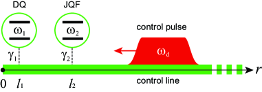
In this study, we propose a filter that prohibits radiative decay of the qubit into the contorl line while not affecting the control speed. Figure 1 is the schematic of the considered setup: a data qubit (DQ) to be controlled is coupled to an end of a semi-infinite control line, and a filter qubit, which is referred to as the Josephson quantum filter (JQF), is placed at a distance of the order of the resonance wavelength of DQ. In such waveguide-QED setups, it is known that a qubit functions as a nonlinear mirror, which completely reflects a weak field due to destructive interference and transmits a stronger field due to absorption saturation shen2005a ; shen2005b ; astafiev2010 . In radiative decay of DQ, where only a single photon concerns, JQF works as a mirror that prohibits radiative decay of DQ. On the other hand, when we perform gate operations on DQ by applying strong control pulses, JQF transmits the pulses and does not reduce the gate speed. Since JQF is a passive circuit element which is free from active control on it, JQF is ready to be incorporated in complicated circuits involving many qubits. Together with the established schemes such as Purcell filters reed2010 ; jeffrey2014 ; Sete2015 ; walter2017 and tunable qubit-waveguide couplers sete2013catch ; bockstiegel2016tunable ; forn2017demand , JQF would be highly useful for constructing a network of long-lived qubits yet allowing fast control and measurements.

The rest of this paper is organized as follows. In Sec. II, we theoretically describe the considered setup. We present the Hamiltonian of the overall system composed of DQ, JQF and a semi-infinite control line, and derive their Heisenberg equations. In Sec. III, assuming the absence of JQF, we review the trade-off between the gate speed and the lifetime of DQ. In Sec. IV, we analyze radiative decay of initially excited DQ. We derive an analytic formula of the radiative decay rate of DQ and clarify the condition that JQF protects DQ from radiative decay. In Sec. V, we numerically examine the microwave response of DQ and JQF to confirm the following: JQF does not affect the dynamics of DQ induced by the control field and therefore does not reduce the gate speed. At the same time, JQF prohibits radiative decay of DQ while the control field is off. Section VI is devoted to the summary.

II Formulation

II.1 Hamiltonian

The physical setup considered in this study is schematically illustrated in Fig. 1. In order to apply control microwave pulses to DQ (qubit 1), we attach a semi-infinite waveguide to DQ. In front of DQ, we attach JQF (qubit 2), which is also a qubit with the same frequency as DQ. The semi-infinite waveguide extends in the $r>0$ region. Its eigenmodes are standing waves, which are continuously labeled by a wavenumber $k(>0)$. Assuming the open boundary condition at the termination point ($r=0$), the mode function $f_{k}(r)$ is given by

$$f_{k}(r) = \sqrt{\frac{2}{\pi}}\cos kr.$$ (1)

We denote the annihilation operator for this mode by $\hat{b}_{k}$. The mode functions are normalized as $\int_{0}^{\infty}drf^{*}_{k^{\prime}}(r)f_{k}(r)=\delta(k-k^{\prime})$.

Both qubits can be regarded as two-level systems. We denote the lowering operator of qubit $m$ ($m=1,2$) by $\hat{\sigma}_{m}$, the transition frequency by $\omega_{m}$, the coupling position to the waveguide by $l_{m}$ and the coupling strength by $\gamma_{m}$. Note that $\gamma_{m}$ represents the radiative decay rate of qubit $m$, assuming that the qubit is coupled to an infinite waveguide.

Setting $\hbar=v=1$, where $v$ is the microwave velocity in the waveguide, the Hamiltonian of the overall system composed of DQ, JQF, and the semi-infinite waveguide is given by

$$\hat{H} = \sum_{m}\omega_{m}\hat{\sigma}_{m}^{{\dagger}}\hat{\sigma}_{m}+\int_{0}^{\infty}dk\ \left[k\hat{b}_{k}^{{\dagger}}\hat{b}_{k}+\textstyle{\sum}_{m}g_{mk}(\hat{\sigma}_{m}^{{\dagger}}\hat{b}_{k}+\hat{b}_{k}^{{\dagger}}\hat{\sigma}_{m})\right],$$ (2)

where the coupling constant $g_{mk}$ is given by

$$g_{mk} = \sqrt{\frac{\gamma_{m}}{2}}f_{k}(l_{m})=\sqrt{\frac{\gamma_{m}}{\pi}}\cos(kl_{m}).$$ (3)

In this study, we aim to protect DQ from radiative decay using JQF. For this purpose, the system parameters are chosen as follows. (i) The two qubits are nearly resonant, i.e., $\omega_{1}\approx\omega_{2}\approx\omega_{q}$. (ii) The positions $l_{1}$ and $l_{2}$ of the qubits are of the order of their resonance wavelength, $\lambda_{q}=2\pi v/\omega_{q}$. DQ is closer to the end of the waveguide than JQF, i.e., $0\leq l_{1}\leq l_{2}$. (iii) The coupling between JQF and the waveguide is much stronger than that of DQ, i.e., $\gamma_{1}\ll\gamma_{2}$. Unless otherwise specified, we employ the parameter values listed in the caption of Fig. 1.

For a semi-infinite waveguide, the wavenumber $k$ of the waveguide mode is restricted to be positive. However, we formally extend the lower limit of $k$ to $-\infty$ , and introduce the real-space representation $\widetilde{b}_{r}$ of the field operator by

$$\widetilde{b}_{r} = \frac{1}{\sqrt{2\pi}}\int_{-\infty}^{\infty}dk\ e^{ikr}\hat{b}_{k}.$$ (4)

The space variable $r$ runs over $-\infty<r<\infty$: the negative (positive) region represents the incoming (outgoing) field. The introduction of the real-space representation has been validated by a rigorous “modes of the universe” approach gea2013space .

II.2 Heisenberg equations

The Heisenberg equation for $\hat{b}_{k}$ is given by $\frac{d}{dt}\hat{b}_{k}=-ik\hat{b}_{k}-i\sum_{m}g_{mk}\hat{\sigma}_{m}$. This is formally solved as

$$\hat{b}_{k}(t) = \hat{b}_{k}(0)e^{-ikt}-i\sum_{m}g_{mk}\int_{0}^{t}dt^{\prime}\hat{\sigma}_{m}(t^{\prime})e^{ik(t^{\prime}-t)}.$$ (5)

Switching to the real-space representation with Eq. (4), we have

$$\widetilde{b}_{r}(t) = \widetilde{b}_{r-t}(0)-i\sum_{m}\sqrt{\frac{\gamma_{m}}{2}}\left[\Theta_{r\in(-l_{m},t-l_{m})}\hat{\sigma}_{m}(t-r-l_{m})+\Theta_{r\in(l_{m},t+l_{m})}\hat{\sigma}_{m}(t-r+l_{m})\right],$$ (6)

where $\Theta$ is a product of the step functions, $\Theta_{r\in(a,b)}=\theta(r-a)\theta(b-r)$. This equation plays the role of the input-output relation in quantum optics gardiner2004 ; walls2007 .

The Heisenberg equation for a system operator $\hat{o}$ (composed of $\hat{\sigma}_{1}$, $\hat{\sigma}_{2}$ and their conjugates) is written, from Eqs. (2) and (4), as

$$\frac{d}{dt}\hat{o} = i[\hat{H}_{s},\hat{o}]+i\sum_{m}\sqrt{\frac{\gamma_{m}}{2}}\left([\hat{\sigma}_{m}^{{\dagger}},\hat{o}]\left\{\widetilde{b}_{l_{m}}(t)+\widetilde{b}_{-l_{m}}(t)\right\}+\left\{\widetilde{b}_{l_{m}}^{{\dagger}}(t)+\widetilde{b}_{-l_{m}}^{{\dagger}}(t)\right\}[\hat{\sigma}_{m},\hat{o}]\right),$$ (7)

where $\hat{H}_{s}=\sum_{m}\omega_{m}\hat{\sigma}_{m}^{{\dagger}}\hat{\sigma}_{m}$. From Eq. (6), we obtain the following equality:

$$\widetilde{b}_{l_{m}}(t)+\widetilde{b}_{-l_{m}}(t) = \widetilde{b}_{l_{m}-t}(0)+\widetilde{b}_{-l_{m}-t}(0)-i\sum_{n}\sqrt{\frac{\gamma_{n}}{2}}\left[\hat{\sigma}_{n}(t-l_{m}-l_{n})+\hat{\sigma}_{n}(t-|l_{m}-l_{n}|)\right].$$ (8)

From Eqs. (7) and (8), we have

$$\frac{d}{dt}\hat{o} = i[\hat{H}_{s},\hat{o}]+i\sum_{m}\left\{[\hat{\sigma}_{m}^{{\dagger}},\hat{o}]\hat{N}_{m}(t)+\hat{N}^{{\dagger}}_{m}(t)[\hat{\sigma}_{m},\hat{o}]\right\}$$ (9)

$$+ \sum_{m,n}\frac{\sqrt{\gamma_{m}\gamma_{n}}}{2}[\hat{\sigma}_{m}^{{\dagger}},\hat{o}]\left\{\hat{\sigma}_{n}(t-l_{m}-l_{n})+\hat{\sigma}_{n}(t-|l_{m}-l_{n}|)\right\}$$

$$- \sum_{m,n}\frac{\sqrt{\gamma_{m}\gamma_{n}}}{2}\left\{\hat{\sigma}_{n}^{{\dagger}}(t-l_{m}-l_{n})+\hat{\sigma}_{n}^{{\dagger}}(t-|l_{m}-l_{n}|)\right\}[\hat{\sigma}_{m},\hat{o}].$$

Note that the explicit time dependence is omitted for operators at time $t$, and the operators with negative time variable should be replaced with zero. The noise operator $\hat{N}_{m}(t)$ for qubit $m$ is defined by

$$\hat{N}_{m}(t) = \sqrt{\frac{\gamma_{m}}{2}}\left[\widetilde{b}_{l_{m}-t}(0)+\widetilde{b}_{-l_{m}-t}(0)\right].$$ (10)

II.3 Free-evolution approximation

The Heisenberg equation (9), which is rigorously driven from the Hamiltonian of Eq. (2), contains qubit operators with retarded times. However, considering that the qubit decay during such retardation is negligibly small ($\gamma_{j}l_{j}/v\ll 1$), we can employ the free-evolution approximation johansson2008 ; koshino2012 , $\hat{\sigma}_{j}(t-\Delta t)\approx e^{i\omega_{q}\Delta t}\hat{\sigma}_{j}(t)$. The validity of this approximation is confirmed in Appendix A. Then, Eq. (9) is recast into the following simpler form:

$$\frac{d}{dt}\hat{o} = i[\hat{H}_{s},\hat{o}]+i\sum_{m}\left\{[\hat{\sigma}_{m}^{{\dagger}},\hat{o}]\hat{N}_{m}(t)+\hat{N}^{{\dagger}}_{m}(t)[\hat{\sigma}_{m},\hat{o}]\right\}+\sum_{m,n}\left(\xi_{mn}[\hat{\sigma}_{m}^{{\dagger}},\hat{o}]\hat{\sigma}_{n}-\xi^{*}_{mn}\hat{\sigma}_{n}^{{\dagger}}[\hat{\sigma}_{m},\hat{o}]\right),$$ (11)

$$\xi_{mn} = \frac{\sqrt{\gamma_{m}\gamma_{n}}}{2}\left(e^{i\omega_{q}(l_{m}+l_{n})}+e^{i\omega_{q}|l_{m}-l_{n}|}\right).$$ (12)

Although the direct interaction between DQ and JQF is absent in the Hamiltonian of Eq. (2), virtual waveguide photons mediate an effective interaction between them, which appears as $\xi_{12}=\xi_{21}=\sqrt{\gamma_{1}\gamma_{2}}\cos(\omega_{q}l_{1})e^{i\omega_{q}l_{2}}$. Note that the roles of DQ and JQF are asymmetric in this interaction due to the semi-infiniteness of the control line.

Since the detuning of the control pulse from the qubit resonance, $\omega_{d}-\omega_{q}$, is small enough to satisfy $(\omega_{d}-\omega_{q})l_{j}/v\ll 1$ in the considered setup, we can make the following approximation, $\widetilde{b}_{\Delta r-t}(0)\approx e^{i\omega_{q}\Delta r}\widetilde{b}_{-t}(0)$. Then we have

$$\hat{N}_{j}(t) = \sqrt{2\gamma_{j}}\cos(\omega_{q}l_{j})\widetilde{b}_{-t}(0).$$ (13)

For future reference, setting $\hat{o}=\hat{\sigma}_{1}$, we have

$$\frac{d}{dt}\hat{\sigma}_{1} = (-i\omega_{q}-\xi_{11})\hat{\sigma}_{1}-\xi_{12}(1-2\hat{\sigma}_{1}^{{\dagger}}\hat{\sigma}_{1})\hat{\sigma}_{2}+i(1-2\hat{\sigma}_{1}^{{\dagger}}\hat{\sigma}_{1})\hat{N}_{1}(t).$$ (14)

II.4 Effective interaction and cooperative dissipator

In the preceding theoretical works dealing with the qubit system coupled to an infinite waveguide chang2012 ; lalumiere2013 ; van2013 ; konyk2017 , the photon-mediated qubit-qubit interaction is treated by the effective dipole exchange interaction $\hat{H}_{e}$ and the cooperative dissipator $\hat{S}$. Here, we rewrite Eqs. (11) and (12) in this form for reference. Dividing $\xi_{mn}$ into the real and imaginary parts, we have

$$\frac{d}{dt}\hat{o} = i[\hat{H}_{s}+\hat{H}_{e},\hat{o}]+\frac{[\hat{S}^{{\dagger}},\hat{o}]\hat{S}+\hat{S}^{{\dagger}}[\hat{o},\hat{S}]}{2}+i\left\{\hat{b}_{\mathrm{in}}^{{\dagger}}(t)[\hat{S},\hat{o}]+[\hat{S}^{{\dagger}},\hat{o}]\hat{b}_{\mathrm{in}}(t)\right\},$$ (15)

$$\hat{H}_{e} = \sum_{m,n}J_{mn}\hat{\sigma}_{m}^{{\dagger}}\hat{\sigma}_{n},$$ (16)

$$\hat{S} = \sum_{m}\sqrt{2\gamma_{m}}\cos(\omega_{q}l_{m})\hat{\sigma}_{m},$$ (17)

$$J_{mn} = \sqrt{\gamma_{m}\gamma_{n}}\cos[\omega_{0}\min(l_{m},l_{n})]\sin[\omega_{0}\max(l_{m},l_{n})].$$ (18)

where $\hat{b}_{\mathrm{in}}(t)=\widetilde{b}_{-t}(0)$. Three comments are in order regarding the above equations. (i) The cooperative dissipator $\hat{S}$ and the effective interaction $\hat{H}_{e}$ result from the real and imaginary parts of $\xi_{mn}$, respectively. (ii) In the case of an infinite waveguide, there appears two kinds of cooperative dissipators corresponding to the positively and negatively propagating modes. Here, the cooperative dissipator $\hat{S}$ is unique, and the cosine function appearing in $\hat{S}$ results from the standing-wave mode function [Eq. (1)]. (iii) In the case of an infinite waveguide, the coefficient $J_{mn}$ of the effective interaction depends only on the mutual distance between the qubits, $|l_{m}-l_{n}|$. Here, $J_{mn}$ has a more complicated form due to the semi-infiniteness of the waveguide.

III Trade-off between qubit lifetime and gate speed

In this section, we observe the trade-off between the lifetime of DQ and the gate speed, assuming the absence of JQF ($\gamma_{2}=0$). The Heisenberg equation (14) for $\hat{\sigma}_{1}$ is then rewritten as

$$\frac{d}{dt}\hat{\sigma}_{1} = (-i\overline{\omega}_{q}-\eta^{2}/2)\hat{\sigma}_{1}+i\eta(1-2\hat{\sigma}_{1}^{{\dagger}}\hat{\sigma}_{1})\widetilde{b}_{-t}(0),$$ (19)

where $\overline{\omega}_{q}=\omega_{q}+(\gamma_{1}/2)\sin(2\omega_{q}l_{1})$ is the renormalized qubit frequency including the Lamb shift. A real constant $\eta=\sqrt{2\gamma_{1}}\cos(\omega_{q}l_{1})$ has two roles that originate in the fluctuation-dissipation theorem: the radiative decay rate of the qubit and the coupling between the qubit and the applied field.

In the absence of the input field, the qubit excitation probability decays as $\frac{d}{dt}\langle\hat{\sigma}_{1}^{{\dagger}}\hat{\sigma}_{1}\rangle=-\eta^{2}\langle\hat{\sigma}_{1}^{{\dagger}}\hat{\sigma}_{1}\rangle$. Therefore, the qubit radiative lifetime $T_{r}$ is given by

$$T_{r} = \frac{1}{\eta^{2}}.$$ (20)

Note that, when coupled to a semi-infinite waveguide, the radiative lifetime depends on the qubit position $l_{1}$ due to the broken translation symmetry. On the other hand, when we apply a resonant control field $E_{\mathrm{in}}(t)=E_{d}e^{-i\overline{\omega}_{q}t}$ through the waveguide, the qubit excitation probability evolves as $\frac{d^{2}}{dt^{2}}\langle\hat{\sigma}_{1}^{{\dagger}}\hat{\sigma}_{1}\rangle=2\eta^{2}|E_{d}|^{2}(1-2\langle\hat{\sigma}_{1}^{{\dagger}}\hat{\sigma}_{1}\rangle)$, and exhibits the Rabi oscillation with the Rabi frequency of $\Omega_{R}=2\eta|E_{d}|$. Therefore, the gate speed $T_{g}^{-1}$ for a $\pi$-pulse is given by

$$T_{g}^{-1} = \frac{2\eta|E_{d}|}{\pi}.$$ (21)

Thus, there exists a trade-off between the qubit radiative lifetime and the gate speed. The overall lifetime $T_{1}$ of the qubit is always shorter than the radiative lifetime $T_{r}$ due to other relaxation channels. Therefore, from Eqs. (20) and (21), we have the following inequality,

$$T_{1}\left(\frac{1}{T_{g}}\right)^{2}\leq\frac{4|E_{d}|^{2}}{\pi^{2}}.$$ (22)

$|E_{d}|^{2}$ in the right-hand side represents the photon rate of the applied field. This is limited, besides the practical reasons, by the finite anharmonicity of the qubit, which is particularly small for the transmon-type qubits.

IV Radiative decay

In this section, we analytically investigate the radiative decay of DQ in the presence of JQF and clarify the optimal condition for JQF. As the initial state, we consider a state in which only DQ is excited. The state vector is written as

$$|\psi(0)\rangle = \hat{\sigma}_{1}^{{\dagger}}|v\rangle,$$ (23)

where $|v\rangle$ represents the vacuum state of the whole setup. Since the Hamiltonian of Eq. (2) conserves the total excitation number, the state vector at time $t$, $|\psi(t)\rangle=e^{-i\hat{H}t}|\psi(0)\rangle$, is written as follows:

$$|\psi(t)\rangle = \sum_{j=1,2}\alpha_{j}(t)\hat{\sigma}_{j}^{{\dagger}}|v\rangle+\int dr\ f(r,t)\widetilde{b}_{r}^{{\dagger}}|v\rangle,$$ (24)

where the coefficients $\alpha_{j}(t)$ and the wavepacket of the emitted photon $f(r,t)$ satisfy the normalization condition of $\sum_{j}|\alpha_{j}(t)|^{2}+\int_{0}^{t}dr|f(r,t)|^{2}=1$. Using the fact that $\hat{H}|v\rangle=0$, we have $\alpha_{j}(t)=\langle v|\hat{\sigma}_{j}|\psi(t)\rangle=\langle v|\hat{\sigma}_{j}(t)\hat{\sigma}_{1}^{{\dagger}}(0)|v\rangle$. From Eq. (14) and its counterpart for $\hat{\sigma}_{2}(t)$, the equations of motion for $\alpha_{j}(t)$ are given by

$$\frac{d\alpha_{1}}{dt} = -(i\omega_{q}+\xi_{11})\alpha_{1}-\xi_{12}\alpha_{2},$$ (25)

$$\frac{d\alpha_{2}}{dt} = -\xi_{21}\alpha_{1}-(i\omega_{q}+\xi_{22})\alpha_{2}.$$ (26)

with the initial conditions of $\alpha_{1}(0)=1$ and $\alpha_{2}(0)=0$. In deriving the above equations, we used $\hat{N}_{j}(t)|\psi(0)\rangle=0$ and $\hat{\sigma}_{1}(t)\hat{\sigma}_{2}(t)\hat{\sigma}_{j}^{{\dagger}}(0)|v\rangle=0$. For reference, the wavepacket of the emitted photon is given by $f(r,t)=-i\sqrt{2\gamma_{1}}\cos(\omega_{q}l_{1})\alpha_{1}(t-r)-i\sqrt{2\gamma_{2}}\cos(\omega_{q}l_{2})\alpha_{2}(t-r)$ for $0\leq r\leq t$, and $f(r,t)=0$ otherwise.

IV.1 Decay rate of DQ

In the absence of the photon-mediated interaction between qubits, the complex frequency of qubit $j$ is given by $\widetilde{\omega}_{j}=\omega_{q}-i\xi_{jj}$, and the radiative decay rate is given by $-2\mathrm{Im}(\widetilde{\omega}_{j})=2\gamma_{j}\cos^{2}(\omega_{q}l_{j})$. Therefore, except for the special case of $l_{2}\approx\frac{1+2n}{4}\lambda_{q}$ ($n=0,1,\cdots$), where $\lambda_{q}=2\pi v/\omega_{q}$ is the resonance wavelength of the qubits, JQF decays much faster than DQ. Then, by switching to the frame rotating at $\omega_{q}$ and applying the adiabatic approximation, Eq. (26) reduces to $\alpha_{2}(t)\approx-(\xi_{21}/\xi_{22})\alpha_{1}(t)$. Substituting this into Eq. (25), we confirm that the complex frequency $\widetilde{\omega}_{1}^{\prime}$ of DQ reduces to a real quantity:

$$\widetilde{\omega}_{1}^{\prime} = \omega_{q}-\gamma_{1}\frac{\cos(\omega_{q}l_{1})\sin[\omega_{q}(l_{2}-l_{1})]}{\cos(\omega_{q}l_{2})}.$$ (27)

This implies that, owing to JQF, DQ acquires an infinite radiative lifetime regardless of its position $l_{1}(<l_{2})$.

For comparison, we consider the case of $l_{1}>l_{2}$. The renormalized complex frequency of DQ is then given by

$$\widetilde{\omega}_{1}^{\prime\prime} = \omega_{q}-\gamma_{1}e^{i\omega_{q}(l_{1}-l_{2})}\sin[\omega_{q}(l_{1}-l_{2})],$$ (28)

the imaginary part of which vanishes only when $\sin[\omega_{q}(l_{1}-l_{2})]=0$. Therefore, in contrast with the case of $l_{1}<l_{2}$, the radiative decay of DQ is prohibited only when the DQ locates exactly at $l_{1}=l_{2}+n\lambda_{q}/2$ ($n=0,1,\cdots$).

These results can be understood intuitively by assuming that JQF functions as an “atomic mirror” and imposes a closed boundary condition on the waveguide field at $r=l_{2}$. Then, in the $0\leq r\leq l_{2}$ region, JQF forms an effective cavity whose eigenfrequencies are $\omega^{\mathrm{eff}}_{n}=(\frac{1}{2}+n)\pi/l_{2}$. The decay of DQ is prohibited as long as $\omega_{q}\neq\omega^{\mathrm{eff}}_{n}$. On the other hand, in the $r\geq l_{2}$ region, the eigenmode spectrum is continuous due to the semi-infiniteness of the waveguide. The vacuum fluctuation of the waveguide field at the qubit frequency $\omega_{q}$ vanishes at $r=l_{2}+n\lambda_{q}/2$ ($n=0,1,\cdots$) because the eigenmode function is a standing wave having a node at $r=l_{2}$. The decay of DQ is prohibited only when it locates there.

The effect of the intrinsic decay of JQF other than the radiative decay into the line, which is assumed to be absent throughout this paper, is discussed in Appendix B. It is revealed there that the radiative decay rate of DQ is suppressed by a factor of $\gamma_{\mathrm{i}2}/\gamma_{2}$, where $\gamma_{\mathrm{i}2}$ ($\gamma_{2}$) is the intrinsic (radiative) decay rate of JQF. Therefore, the suppression becomes imperfect when JQF has a finite intrinsic decay rate, but is still substantial if $\gamma_{\mathrm{i}2}\ll\gamma_{2}$.

IV.2 Time evolution

Figure 2: Survival probability of DQ, $P_{1}(t)=|\alpha_{1}(t)|^{2}$. The parameter values are described in the caption of Fig. 1, except that the JQF position $l_{2}$ is varied. (a) Results for $l_{2}/\lambda_{q}=0.5$ (red solid) and $0.35$ (green dashed). (b) Results for $l_{2}/\lambda_{q}=0.25$ (red solid) and $0.245$ (green dashed). The free survival probability in the absence of JQF is also shown (blue dotted).

The solution of Eqs. (25) and (26) are given by

$$\alpha_{1}(t) = \left(\frac{\mu_{2}+\xi_{11}}{\mu_{2}-\mu_{1}}e^{\mu_{1}t}+\frac{\mu_{1}+\xi_{11}}{\mu_{1}-\mu_{2}}e^{\mu_{2}t}\right)e^{-i\omega_{q}t},$$ (29)

$$\alpha_{2}(t) = \frac{\xi_{21}}{\mu_{2}-\mu_{1}}(e^{\mu_{1}t}-e^{\mu_{2}t})e^{-i\omega_{q}t},$$ (30)

where $\mu_{1}$ and $\mu_{2}$ are defined by

$$(z+\xi_{11})(z+\xi_{22})-\xi_{12}\xi_{21}=(z-\mu_{1})(z-\mu_{2}).$$ (31)

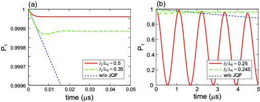
The survival probability of DQ is given by $P_{1}(t)=|\alpha_{1}(t)|^{2}$. In Fig. 2, fixing the position of DQ at $l_{1}=0$, time evolution of $P_{1}(t)$ is shown for several values of $l_{2}$. Expectedly, we observe that the decay of DQ is suppressed, except when $l_{2}\approx\frac{1+2n}{4}\lambda_{q}$. The optimal position of JQF is $l_{2}=n\lambda_{q}/2$. Equations (29) and (30) then reduce to the following forms:

$$\alpha_{1}(t) = \left(\frac{\gamma_{2}}{\gamma_{1}+\gamma_{2}}+\frac{\gamma_{1}}{\gamma_{1}+\gamma_{2}}e^{-(\gamma_{1}+\gamma_{2})t}\right)e^{-i\omega_{q}t},$$ (32)

$$\alpha_{2}(t) = (-)^{n+1}\frac{\sqrt{\gamma_{1}\gamma_{2}}}{\gamma_{1}+\gamma_{2}}[1-e^{-(\gamma_{1}+\gamma_{2})t}]e^{-i\omega_{q}t}.$$ (33)

In the $t\to\infty$ limit, $P_{1}(t)=(\frac{\gamma_{2}}{\gamma_{1}+\gamma_{2}})^{2}\approx 1-\frac{2\gamma_{1}}{\gamma_{2}}$. Therefore, the radiative decay of DQ is mostly prohibited when $\gamma_{2}\gg\gamma_{1}$.

Such prohibited decay of DQ originates in the subradiance effect goban2015 ; ostermann2019 ; albrecht2019 . This is understood most clearly in the case of $l_{1}=l_{2}=0$. From the Hamiltonian of Eq. (2), we observe that the following two states, $|\mathrm{sup}\rangle$ and $|\mathrm{sub}\rangle$, respectively correspond to the super- and sub-radiant states within the one-excitation subspace of the two qubits:

$$|\mathrm{sup}\rangle = \frac{\sqrt{\gamma_{1}}\hat{\sigma}_{1}^{{\dagger}}+\sqrt{\gamma_{2}}\hat{\sigma}_{2}^{{\dagger}}}{\sqrt{\gamma_{1}+\gamma_{2}}}|v\rangle,$$ (34)

$$|\mathrm{sub}\rangle = \frac{\sqrt{\gamma_{2}}\hat{\sigma}_{1}^{{\dagger}}-\sqrt{\gamma_{1}}\hat{\sigma}_{2}^{{\dagger}}}{\sqrt{\gamma_{1}+\gamma_{2}}}|v\rangle.$$ (35)

The superradiant state decays rapidly with a rate of $2(\gamma_{1}+\gamma_{2})$, whereas the subradiant state is an eigenstate of the Hamiltonian and does not decay. The excited state of DQ is mostly composed of the subradiant state and contains a tiny fraction of the superradiant state,

$$\hat{\sigma}_{1}^{{\dagger}}|v\rangle = \frac{\sqrt{\gamma_{1}}|\mathrm{sup}\rangle+\sqrt{\gamma_{2}}|\mathrm{sub}\rangle}{\sqrt{\gamma_{1}+\gamma_{2}}}.$$ (36)

The rapid decay of the superradiant component is observed as the initial drop of the survival probability in Fig. 2(a). The quasi-stationary $P_{1}\,[=\gamma_{2}^{2}/(\gamma_{1}+\gamma_{2})^{2}]$ results from the subradiant components. These arguments are compatible with Eqs. (32) and (33) with $n=0$.

V Microwave response

In the previous section, we derived the radiative decay rate of DQ analytically and confirmed that JQF protects DQ from radiative decay through the control line. In this section, we numerically investigate the quantum control of DQ with a microwave pulse applied through the waveguide. We will observe that, as long as the control pulse is sufficiently strong, we can control DQ as if JQF is absent. This implies that JQF does not affect the gate time $T_{g}$ of DQ while enhancing its lifetime $T_{1}$, and thus breaks the trade-off relation of Eq.(22).

We assume that both qubits are in the ground state at the initial moment ($t=0$), and a classical control field $E_{\mathrm{in}}(t)$ is applied through the waveguide for $t>0$. The spatial waveform of the control field at $t=0$ is $E_{\mathrm{in}}(-r)$. Therefore, the initial state vector is written as

$$|\phi(0)\rangle = {\cal N}\exp\left(\int_{-\infty}^{0}\!\!dr\ E_{\mathrm{in}}(-r)\widetilde{b}_{r}^{{\dagger}}\right)|v\rangle,$$ (37)

where ${\cal N}=\exp\left(-\int dr|E_{\mathrm{in}}(-r)|^{2}/2\right)$ is a normalization factor. Note that this is in a coherent state and therefore is an eigenvector of the noise operator, Eq. (13). Hereafter, we use the notation of $\langle\phi(0)|\hat{A}(t)|\phi(0)\rangle=\langle\hat{A}(t)\rangle$. From Eqs. (14) and (37), the equation of motion for $\langle\hat{\sigma}_{1}(t)\rangle$ is given by

$$\frac{d}{dt}\langle\hat{\sigma}_{1}\rangle = (-i\omega_{q}-\xi_{11})\langle\hat{\sigma}_{1}\rangle-\xi_{12}\langle\hat{\sigma}_{2}\rangle+2\xi_{12}\langle\hat{\sigma}_{1}^{{\dagger}}\hat{\sigma}_{1}\hat{\sigma}_{2}\rangle+i(1-2\langle\hat{\sigma}_{1}^{{\dagger}}\hat{\sigma}_{1}\rangle)\langle\hat{N}_{1}(t)\rangle,$$ (38)

where

$$\langle\hat{N}_{j}(t)\rangle = \sqrt{2\gamma_{j}}\cos(\omega_{q}l_{j})E_{\mathrm{in}}(t).$$ (39)

We numerically solve the simultaneous differential equations of the following 9 quantities: $\langle\hat{\sigma}_{1}\rangle$, $\langle\hat{\sigma}_{2}\rangle$, $\langle\hat{\sigma}_{1}^{{\dagger}}\hat{\sigma}_{1}\rangle$, $\langle\hat{\sigma}_{2}^{{\dagger}}\hat{\sigma}_{2}\rangle$, $\langle\hat{\sigma}_{2}^{{\dagger}}\hat{\sigma}_{1}\rangle$, $\langle\hat{\sigma}_{1}\hat{\sigma}_{2}\rangle$, $\langle\hat{\sigma}_{1}^{{\dagger}}\hat{\sigma}_{1}\hat{\sigma}_{2}\rangle$, $\langle\hat{\sigma}_{2}^{{\dagger}}\hat{\sigma}_{1}\hat{\sigma}_{2}\rangle$, and $\langle\hat{\sigma}_{1}^{{\dagger}}\hat{\sigma}_{2}^{{\dagger}}\hat{\sigma}_{1}\hat{\sigma}_{2}\rangle$.

V.1 Rabi oscillation

Figure 3: Rabi oscillations of DQ ($P_{1}$, red solid) and JQF ($P_{2}$, blue dotted). The free Rabi oscillation of DQ ($P_{1f}$, green dashed) in the absence of JQF is also shown for reference. The Rabi frequency is set at $\Omega_{1}/2\pi=2.5$ MHz in (a), and $25$ MHz in (b). The corresponding photon rates are $|E_{d}|^{2}/\gamma_{2}=3.91$ and $391$, respectively. $P_{1}$ and $P_{1f}$ are almost overlapping in (b).

First, we investigate the case of continuous drive,

$$E_{\mathrm{in}}(t) = \begin{cases}0&(t<0)\\ E_{d}e^{-i\omega_{d}t}&(t\geq 0)\end{cases},$$ (40)

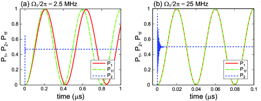
and observe the Rabi oscillations of DQ and JQF induced by this drive field. Note that $|E_{d}|^{2}$ represents the incoming photon rate. In the numerical simulations, we assume that both DQ and JQF are placed at their optimal positions ($l_{1}=0$, $l_{2}=\lambda_{q}/2$) and that a resonant drive field ($\omega_{d}=\omega_{q}$) is applied through the waveguide.

In Fig. 3, the excitation probabilities of DQ and JQF, $P_{j}(t)=\langle\hat{\sigma}_{j}^{{\dagger}}\hat{\sigma}_{j}\rangle$, are plotted for various drive power. In order to emphasize the effect of JQF on DQ, we also plot the free Rabi oscillation of DQ, $P_{1f}(t)$, assuming the absence of JQF. $P_{1f}(t)$ is analytically given by

$$P_{1f}(t) = \frac{\Omega_{1}^{2}}{2(\Omega_{1}^{2}+2\gamma_{1}^{2})}\left[1-e^{-3\gamma_{1}t/2}\left(\cos\widetilde{\Omega}_{1}t+\frac{3\gamma_{1}}{2\widetilde{\Omega}_{1}}\sin\widetilde{\Omega}_{1}t\right)\right],$$ (41)

where $\Omega_{1}=\sqrt{8\gamma_{1}|E_{d}|^{2}}$ (Rabi frequency) and $\widetilde{\Omega}_{1}=\sqrt{8\gamma_{1}|E_{d}|^{2}-(\gamma_{1}/2)^{2}}$. We observe that $P_{1}(t)$ and $P_{1f}(t)$ are almost overlapping for a strong drive satisfying $\gamma_{2}\ll|E_{d}|^{2}$. Thus, the Rabi oscillation of DQ is almost unaffected by JQF. This is explained as follows: In the right-hand-side of Eq. (14), we see that DQ is driven by two different mechanisms: the mutual interaction between DQ and JQF (second term) and the applied field (third term). Therefore, the condition that the Rabi oscillation of DQ is unaffected by JQF is $|\xi_{12}|\ll\langle\hat{N}_{1}(t)\rangle$, which reduces to $\gamma_{2}\ll|E_{d}|^{2}$.

On the other hand, JQF undergoes a much faster Rabi oscillation than DQ ($\Omega_{2}/\Omega_{1}=\sqrt{\gamma_{2}/\gamma_{1}}\approx 224$), and relaxes to its stationary value of $\Omega_{2}^{2}/2(\Omega_{2}^{2}+2\gamma_{2}^{2})$ within a relaxation time of $\gamma_{2}^{-1}\sim 5$ ns. For a strong field satisfying $|E_{d}|^{2}\gg\gamma_{2}$, JQF becomes saturated, and the stationary state is approximately the maximally mixed state.

V.2 $\pi$-pulse excitation

Figure 4: Response to $\pi$-pulse. The pulse is on for $0\leq t\leq 20$ ns. (a) Excitation probability of DQ ($P_{1}$, red solid) and JQF ($P_{2}$, blue dotted). The former in the absence of JQF ($P_{1f}$, green dashed) is also plotted. $P_{1}$ and $P_{1f}$ are overlapping for $t\lesssim 0.2\mu\mathrm{s}$. (b) $P_{1}(t)$ for various JQF position $l_{2}$. (c) $P_{1}(t)$ for various JQF frequency $\omega_{2}$. The detuning $\delta\omega$ in the legend is defined by $\delta\omega=\omega_{2}-\omega_{1}$. (d) Dependence of the radiative decay rate of DQ on the detuning.

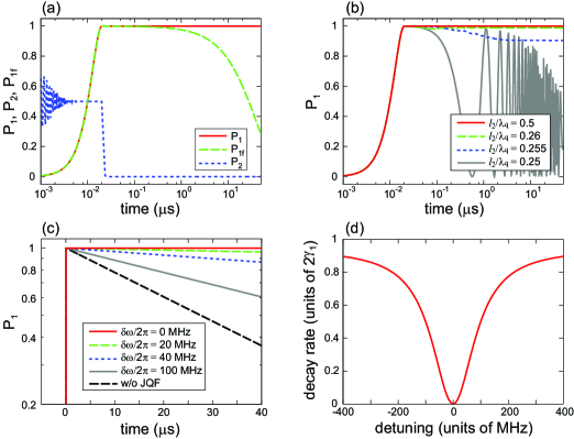
Here we observe the dynamics of DQ and JQF induced by a $\pi$-pulse for DQ. We employ a square $\pi$-pulse with a length of 20 ns ($\Omega_{1}/2\pi=25$ MHz). Time evolution of the excitation probabilities of DQ ($P_{1}$) and JQF ($P_{2}$) are plotted in Fig. 4(a). JQF exhibits a rapid damped Rabi oscillation and relaxes to the maximally mixed state ($P_{2}=1/2$) during $\pi$-pulse irradiation. After the $\pi$-pulse is switched off, JQF quickly decays to the ground state. On the other hand, DQ is excited by the $\pi$-pulse and keeps staying in the excited state even after the $\pi$-pulse is switched off. The stationary value of $P_{1}$ is 0.9997. As we observe later (Fig. 5), damping of DQ is not suppressed completely while the control field is on. The tiny unexcited probability 0.00032 is mainly due to such damping during $\pi$-pulse irradiation.

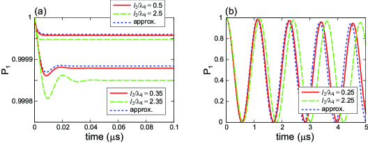
The JQF position $l_{2}$ is varied in Fig. 4(b). A remarkable fact here is that the decay of DQ is prohibited even when JQF is not placed exactly at its optimal position: the stationary excitation probability reaches 0.9994 for $l_{2}/\lambda_{q}=0.35$ (non-optimal), which is comparable to 0.9997 for $l_{2}/\lambda_{q}=0.5$ (optimal). Therefore, the precise positioning of JQF is unnecessary for protection of DQ. This makes practical implementation of the present scheme easier.

The JQF frequency $\omega_{2}$ is varied in Fig. 4(c). We observe that, in the presence of detuning, the protection of DQ by JQF is imperfect, resulting in the exponential decay of DQ. In Fig. 4(d), the DQ decay rate is plotted as a function of the detuning. The functional form of this decay rate is given by Eq. (47). The width of the dip in the decay rate is about 200 MHz, which is determined by the JQF linewidth $\gamma_{2}$.

Figure 5: Comparison of continuous-wave and $\pi$-pulse excitations. The Rabi frequency is set at $\Omega_{1}/2\pi=25$ MHz and the duration of $\pi$ pulse is set at $20$ ns.

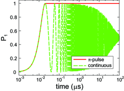
Continuous-wave and $\pi$-pulse excitations are compared in Fig. 5. As we observed in Eq. (41), under continuous-wave excitation, DQ exhibits damped Rabi oscillation with a decay rate of $3\gamma_{1}/2$. This implies that, while the control field is on, the control line works as a dissipation channel and damps the dynamics of DQ. In contrast, after the $\pi$-pulse excitation, DQ stays in the excited state without being dissipated.

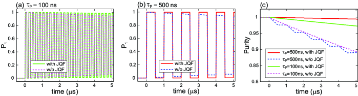
In Fig. 6, we show the bit flips of DQ between the ground and excited states induced by successive $\pi$-pulses. The $\pi$-pulse duration time is set at 20 ns, and the pulse period $\tau_{p}$ is set at 100 ns (duty ratio 0.2) in Fig. 6(a) and at 500 ns (duty ratio 0.04) in Fig. 6(b). Without JQF, the amplitude of $P_{1}$ oscillation damps with a rate around $\gamma_{1}$: $P_{1}$ at $t=5.02~{}\mu$s is 0.9436 in (a) and 0.9417 in (b). The damping rate is almost insensitive to the duty ratio, since damping of DQ always occurs, regardless of the control pulse is on or off. In the presence of JQF, damping of DQ is substantially suppressed: $P_{1}$ at $t=5.02~{}\mu$s reaches 0.9828 in (a) and 0.9968 in (b). Operation with lower duty ratio is more advantageous, since JQF protects DQ only during the control pulse is off. This is also confirmed in Fig. 6(c), which plots time evolution of the purity of DQ, ${\cal P}=\langle\hat{\sigma}_{1}^{{\dagger}}\hat{\sigma}_{1}\rangle^{2}+(1-\langle\hat{\sigma}_{1}^{{\dagger}}\hat{\sigma}_{1}\rangle)^{2}+2|\langle\hat{\sigma}_{1}\rangle|^{2}$.

Figure 6: Successive application of $\pi$-pulses. The $\pi$-pulse duration time is 20 ns. (a) Time evolution of the excitation probability of DQ with the pulse period $\tau_{p}=100$ ns. The green solid (magenta dotted) line shows the results with (without) JQF. (b) The same plot as (a) for $\tau_{p}=500$ ns. The red solid (blue dotted) line shows the results with (without) JQF. (c) Time evolution of the purity of DQ. The upper (lower) two lines show the results with (without) JQF.

VI summary

For scalable quantum information processing, we should perform fast gate operations on the qubits, while keeping long coherence times of the qubits. However, there exists a trade-off between them, which cannot be resolved by a conventional Purcell filter. In this work, we proposed a Josephson quantum filter (JQF), which protects a data qubit (DQ) from radiative decay into the control line without losing the gate speed. In the proposed setup, DQ is coupled to an end of a semi-infinite control line and JQF is coupled to the same line with a distance from DQ of the order of resonance wavelength. Owing to a superradiance effect, JQF suppresses radiative decay of DQ under the following conditions: (i) DQ and JQF are resonant, (ii) JQF couples to the control line by far more strongly than DQ, and (iii) the DQ–JQF distance is close to integer multiples of half of the resonance wavelength. We numerically confirmed that the speed of the gate operations on DQ is unaffected by JQF. The radiative decay of DQ is completely suppressed by JQF when the control field is off, whereas it is not under irradiation of the control field. Thus, the operation of JQF is somewhat similar to that of a tunable coupler between a qubit and a control line. However, JQF is a passive element that is free from active control on it, and therefore is highly suitable for integration in complicated circuits with many qubits.

Appendix A Validation of free-evolution approximation

In this section, in order to check the validity of the free-evolution approximation, we analyze the radiative decay of DQ without the free-evolution approximation. The initial state vector [Eq. (23)] and the state vector at time $t$ [Eq. (24)] remain unchanged in the rigorous analysis. However, without the free-evolution approximation, the equations of motion for $\alpha_{1}(t)$ and $\alpha_{2}(t)$ become delay differential equations. Instead of Eqs. (25) and (26), they are given by

$$\frac{d}{dt}\alpha_{1}(t) = \left(-i\omega_{q}-\frac{\gamma_{1}}{2}\right)\alpha_{1}(t)-\frac{\gamma_{1}}{2}\alpha_{1}(t-2l_{1})-\frac{\sqrt{\gamma_{1}\gamma_{2}}}{2}[\alpha_{2}(t-l_{1}-l_{2})+\alpha_{2}(t+l_{1}-l_{2})],$$ (42)

$$\frac{d}{dt}\alpha_{2}(t) = \left(-i\omega_{q}-\frac{\gamma_{2}}{2}\right)\alpha_{2}(t)-\frac{\gamma_{2}}{2}\alpha_{2}(t-2l_{2})-\frac{\sqrt{\gamma_{1}\gamma_{2}}}{2}[\alpha_{1}(t-l_{1}-l_{2})+\alpha_{1}(t+l_{1}-l_{2})],$$ (43)

with the initial conditions of $\alpha_{1}(0)=1$ and $\alpha_{2}(0)=0$. Note that $\alpha_{1,2}(t)=0$ for $t<0$.

In Fig. 7, fixing $l_{1}(=0)$ and varying $l_{2}$, we compare the rigorous and approximate survival probabilities $P_{1}(t)=|\alpha_{1}(t)|^{2}$. The upper three lines in Fig. 7(a) represent the rigorous ones for $l_{2}/\lambda_{q}=0.5$ and $2.5$ and the approximate one. Note that the free-evolution approximation yields the same $P_{1}(t)$ for $l_{2}/\lambda_{q}=0.5$ and $2.5$. As expected, the agreement between the rigorous and approximate results becomes better for a shorter round-trip time $2l_{2}$. The deviation between the rigorous and approximate $P_{1}(t)$ is negligibly small for $l_{2}/\lambda_{q}=0.5$ ($2.6\times 10^{-6}$ in the stationary state), indicating the validity of the approximation. The lower three lines in Fig. 7(a) and Fig. 7(b) show the results for the non-optimal filter position. The deviation between the rigorous and approximate results are larger in comparison with the optimal cases, but the approximation is fairly good for $l_{2}\lesssim\lambda_{q}$.

Figure 7: Comparison of the rigorous survival probability and the approximate ones based on the free-evolution approximation.

Appendix B Effect of intrinsic loss and detuning

Here, we derive the decay rate of DQ in the presence of the intrinsic loss of DQ and JQF and the detuning between them. We denote the intrinsic decay rates of DQ and JQF by $\gamma_{\mathrm{i1}}$ and $\gamma_{\mathrm{i2}}$, respectively. Then, Eqs. (25) and (26) are modified as follows:

$$\frac{d\alpha_{1}}{dt} = -(i\omega_{1}+\xi_{11}+\gamma_{\mathrm{i1}}/2)\alpha_{1}-\xi_{12}\alpha_{2},$$ (44)

$$\frac{d\alpha_{2}}{dt} = -\xi_{21}\alpha_{1}-(i\omega_{2}+\xi_{22}+\gamma_{\mathrm{i2}}/2)\alpha_{2}.$$ (45)

Switching to the frame rotating at $\omega_{1}$ and solving Eq. (45) adiabatically, the complex frequency of DQ is given by

$$\widetilde{\omega}_{1}^{\prime} = \omega_{q}+i\left(\frac{\xi_{12}\xi_{21}}{\xi_{22}+\gamma_{\mathrm{i2}}/2+i\delta\omega}-\xi_{11}-\frac{\gamma_{\mathrm{i1}}}{2}\right),$$ (46)

where $\delta\omega=\omega_{2}-\omega_{1}$ is the detuning between DQ and JQF. The decay rate of DQ is determined by $\gamma_{DQ}=-2\mathrm{Im}(\widetilde{\omega}_{1})$. For the optimal case of $l_{1}=0$ and $l_{2}=n\lambda_{q}/2$ ($n=0,1,\cdots$), $\gamma_{DQ}$ reduces to the following form:

$$\gamma_{DQ} = \gamma_{\mathrm{i1}}+2\gamma_{1}\left[1-\frac{\gamma_{2}(\gamma_{2}+\gamma_{\mathrm{i2}}/2)}{(\gamma_{2}+\gamma_{\mathrm{i2}}/2)^{2}+(\delta\omega)^{2}}\right].$$ (47)

The first term represents the intrinsic decay rate of DQ, which is unaffected by JQF as expected. The second term represents the radiative decay rate of DQ, which is suppressed by JQF. In the absence of detuning and in the $\gamma_{2}\gg\gamma_{\mathrm{i2}}$ limit, the radiative decay rate of DQ is approximately given by $\gamma_{1}\times(\gamma_{\mathrm{i2}}/\gamma_{\mathrm{2}})$. This implies that, even when JQF has intrinsic loss, we can substantially suppress the radiative decay of DQ by making the radiative decay of JQF dominant. Equation (47) agrees with the Lorentzian dip observed in Fig. 4(d).

References

- (1) R. Barends, J. Kelly, A. Megrant, A. Veitia, D. Sank, E. Jeffrey, T. C. White, J. Mutus, A. G. Fowler, B. Campbell, Y. Chen, Z. Chen, B. Chiaro, A. Dunsworth, C. Neill, P. O’Malley, P. Roushan, A. Vainsencher, J. Wenner, A. N. Korotkov, A. N. Cleland, and J. M. Martinis, Superconducting quantum circuits at the surface code threshold for fault tolerance, Nature 508, 500 (2014).
- (2) J. Kelly, R. Barends, A. G. Fowler, A. Megrant, E. Jeffrey, T. C. White, D. Sank, J. Y. Mutus, B. Campbell, Yu Chen, Z. Chen, B. Chiaro, A. Dunsworth, I.-C. Hoi, C. Neill, P. J. J. O’Malley, C. Quintana, P. Roushan, A. Vainsencher, J. Wenner, A. N. Cleland, and J. M. Martinis, State preservation by repetitive error detection in a superconducting quantum circuit, Nature 519, 66 (2015).
- (3) M. Reagor, C. B. Osborn, N. Tezak, A. Staley, G. Prawiroatmodjo, M. Scheer, N. Alidoust, E. A. Sete, N. Didier, M. P. da Silva, E. Acala, J. Angeles, A. Bestwick, M. Block, B. Bloom, A. Bradley, C. Bui, S. Cald-well, L. Capelluto, R. Chilcott, J. Cordova, G. Crossman, M. Curtis, S. Deshpande, T. E. Bouayadi, D. Girshovich, S. Hong, A. Hudson, P. Karalekas, K. Kuang, M. Lenihan, R. Manenti, T. Manning, J. Marshall, Y. Mohan, W. O’Brien, J. Otterbach, A. Papageorge, J. P. Paquette, M. Pelstring, A. Polloreno, V. Rawat, C. A. Ryan, R. Renzas, N. Rubin, D. Russell, M. Rust, D. Scarabelli, M. Selvanayagam, R. Sinclair, R. Smith, M. Suska, T. W. To, M. Vahidpour, N. Vodrahalli, T. Whyland, K. Yadav, W. Zeng, and C. T. Rigetti, Demonstration of universal parametric entangling gates on a multi-qubit lattice, Sci. Adv. 4, eaao3603 (2018).
- (4) C. Song, K. Xu, H. Li, Y. Zhang, X. Zhang, W. Liu, Q. Guo, Z. Wang, W. Ren, J. Hao, H. Feng, H. Fan, D. Zheng, D. Wang, H. Wang, and S. Zhu, Observation of multi-component atomic Schrödinger cat states of up to 20 qubits, arXiv:1905.00320.
- (5) K. X. Wei, I. Lauer, S. Srinivasan, N. Sundaresan, D. T. McClure, D. Toyli, D. C. McKay, J. M. Gambetta, S. Sheldon, Verifying Multipartite Entangled GHZ States via Multiple Quantum Coherences, arXiv:1905.05720.
- (6) Y. Ye, Z.-Y. Ge, Y. Wu, S. Wang, M. Gong, Y.-R. Zhang, Q. Zhu, R. Yang, S. Li, F. Liang, J. Lin, Y. Xu, C. Guo, L. Sun, C. Cheng, N. Ma, Z. Y. Meng, H. Deng, H. Rong, C.-Y. Lu, C.-Z. Peng, H. Fan, X. Zhu, and J.-W. Pan, Propagation and localization of collective excitations on a 24-qubit superconducting processor, Phys. Rev. Lett. 123, 050502 (2019).
- (7) A. Blais, R.-S. Huang, A. Wallraff, S. M. Girvin, and R. J. Schoelkopf, Cavity quantum electrodynamics for superconducting electrical circuits: An architecture for quantum computation, Phys. Rev. A 69, 062320 (2004).
- (8) R. Vijay, D. H. Slichter, and I. Siddiqi, Observation of quantum jumps in a superconducting artificial atom, Phys. Rev. Lett. 106, 110502 (2011).
- (9) N. Bloembergen, E. M. Purcell, and R. V. Pound, Relaxation effects in nuclear magnetic resonance absorption, Phys. Rev. 73, 679 (1948).
- (10) M. D. Reed, B. R. Johnson, A. A. Houck, L. DiCarlo, J. M. Chow, D. I. Schuster, L. Frunzio, and R. J. Schoelkopf, Fast reset and suppressing spontaneous emission of a superconducting qubit, Appl. Phys. Lett. 96, 203110 (2010).
- (11) E. A. Sete, J. M. Martinis, and A. N. Korotkov, Quantum theory of a bandpass Purcell filter for qubit readout, Phys. Rev. A 92, 012325 (2015).
- (12) D. Sank, E. Jeffrey, J. Y. Mutus, T. C. White, J. Kelly, R. Barends, Y. Chen, Z. Chen, B. Chiaro, A. Dunsworth, A. Megrant, P. J. J. O’Malley, C. Neill, P. Roushan, A. Vainsencher, J. Wenner, A. N. Cleland, and J. M. Martinis, Fast accurate state measurement with superconducting qubits, Phys. Rev. Lett. 112, 190504 (2014).
- (13) T. Walter, P. Kurpiers, S. Gasparinetti, P. Magnard, A. Potocnik, Y. Salathe, M. Pechal, M. Mondal, M. Oppliger, C. Eichler, A. Wallraff, Rapid high-fidelity single-shot dispersive readout of superconducting qubits, Phys. Rev. Appl. 7, 054020 (2017).
- (14) J.-T. Shen and S. Fan, Coherent Single Photon Transport in a One-Dimensional Waveguide Coupled with Superconducting Quantum Bits, Phys. Rev. Lett. 95, 213001 (2005).
- (15) J.-T. Shen and S. Fan, Coherent photon transport from spontaneous emission in one-dimensional waveguides, Opt. Lett. 30, 2001 (2005).
- (16) O. Astafiev, A. M. Zagoskin, A. A. Abdumalikov Jr., Yu. A. Pashkin, T. Yamamoto, K. Inomata, Y. Nakamura, and J. S. Tsai, Resonance fluorescence of a single artificial atom, Science 327, 840 (2010).
- (17) E. A. Sete, A. Galiautdinov, E. Mlinar, J. M. Martinis, and A. N. Korotkov, Catch-disperse-release readout for superconducting qubits, Phys. Rev. Lett. 110, 210501 (2013).
- (18) C. Bockstiegel, Y. Wang, M. R. Vissers, L. F. Wei, S. Chaudhuri, J. Hubmayr, and J. Gao, A tunable coupler for superconducting microwave resonators using a nonlinear kinetic inductance transmission line, Appl. Phys. Lett. 108, 222604 (2016).
- (19) P. Forn-Diaz, C. W. Warren, C. W. S. Chang, A. M. Vadiraj, and C. M. Wilson, On-demand microwave generator of shaped single photons, Phys. Rev. Appl. 8, 054015 (2017).
- (20) J. Gea-Banacloche, Space-time descriptions of quantum fields interacting with optical cavities, Phys. Rev. A 87, 023832 (2013).
- (21) C. W. Gardiner and P. Zoller, Quantum Noise: A Handbook of Markovian and Non-Markovian Quantum Stochastic Methods with Applications to Quantum Optics, 3rd ed. (Springer, 2004).
- (22) D. F. Walls and G. J. Milburn, Quantum Optics, 2nd ed. (Springer, Berlin, 2007).
- (23) J. R. Johansson, L. G. Mourokh, A. Yu. Smirnov, and F. Nori, Enhancing the conductance of a two-electron nanomechanical oscillator, Phys. Rev. B 77, 035428 (2008).
- (24) K. Koshino and Y. Nakamura, Control of the radiative level shift and linewidth of a superconducting artificial atom through a variable boundary condition, New J. Phys. 14, 043005 (2012).
- (25) D. E. Chang, L. Jiang, A. V. Gorshkov, and H. J. Kimble, Cavity QED with atomic mirrors, New J. Phys. 14, 063003 (2012).
- (26) K. Lalumiere, B. C. Sanders, A. F. van Loo, A. Fedorov, A. Wallraff, and A. Blais, Input-output theory for waveguide QED with an ensemble of inhomogeneous atoms, Phys. Rev. A 88, 043806 (2013).
- (27) A. F. van Loo, A. Fedorov, K. Lalumiere, B. C. Sanders, A. Blais, and A. Wallraff, Photon-mediated interactions between distant artificial atoms, Science 342, 1494 (2013).
- (28) W. Konyk and J. Gea-Banacloche, One-and two-photon scattering by two atoms in a waveguide, Phys. Rev. A 96, 063826 (2017).
- (29) A. Goban, C.-L. Hung, J. D. Hood, S.-P. Yu, J. A. Muniz, O. Painter, and H. J. Kimble, Superradiance for atoms trapped along a photonic crystal waveguide, Phys. Rev. Lett. 115, 063601 (2015).
- (30) L. Ostermann, C. Meignant, C. Genes, and H. Ritsch, Super- and subradiance of clock atoms in multimode optical waveguides, New J. Phys. 21, 025004 (2019).
- (31) A. Albrecht, L. Henriet, A. Asenjo-Garcia, P. B. Dieterle, O. Painter, and D. E. Chang, Subradiant states of quantum bits coupled to a one-dimensional waveguide, New J. Phys. 21, 025003 (2019).