Benchmark neutrinoless double-beta decay matrix elements in a light nucleus

Abstract

We compute nuclear matrix elements of neutrinoless double-beta decay mediated by light Majorana-neutrino exchange in the $A=6$ system. The goal is to benchmark two many-body approaches, the No-Core Shell Model and the Multi-Reference In-Medium Similarity Renormalization Group. We use the SRG-evolved chiral N3LO-EM500 potential for the nuclear interaction, and make the approximation that isospin is conserved. We compare the results of the two approaches as a function of the cutoff on the many-body basis space. Although differences are seen in the predicted nuclear radii, the ground-state energies and neutrinoless double-beta decay matrix elements produced by the two approaches show significant agreement. We discuss the implications for calculations in heavier nuclei.

I introduction

Since the discovery of the lepton flavor violation in neutrino oscillations (Ahmad et al., 2001; Eguchi et al., 2003; Fukuda et al., 1998), identifying whether the neutrino is a Majorana fermion (i.e. its own antiparticle) has become a priority in nuclear and particle physics. However, because neutrinos are charge neutral and nearly massless, they are notoriously difficult to detect, and their properties remain only partly understood. Major theoretical and experimental collaborative efforts are already underway to study neutrino properties (Martin-Albo et al., 2016; Albert et al., 2014; Gilliss et al., 2018; Gando et al., 2016; Alfonso et al., 2015; Agostini et al., 2017; Aalseth et al., 2018; Andringa et al., 2016; Iwata et al., 2016; Cirigliano et al., 2017; Contessi et al., 2017; Coraggio et al., 2017; Jiao et al., 2017; Tiburzi et al., 2017; Shanahan et al., 2017; Horoi and Neacsu, 2017). Determining whether neutrinos are indeed Majorana particles would not only shed light on the mechanism behind neutrino mass generation, but would also provide insight on leptogenesis and the universe’s apparent matter-antimatter asymmetry.

Neutrinoless double-beta ($0\nu\beta\beta$) decay is a hypothetical lepton-number-violating (LNV) nuclear transition where two neutrons decay to two protons and two electrons but no anti-neutrinos (or the reverse with leptons exchanged with their antiparticles). Observing $0\nu\beta\beta$ decay would confirm the existence of a LNV process, and is commonly viewed as the best means of learning whether neutrinos are Majorana particles. Experiments designed to detect $0\nu\beta\beta$ decay in ton-scale amounts of ${}^{76}\text{Ge}$, ${}^{136}\text{Xe}$, and other materials have already put impressive limits on the $0\nu\beta\beta$-decay half-life (Gilliss et al., 2018; Gando et al., 2016; Agostini et al., 2017), and these limits will only become more accurate as additional data is collected. For a more complete description of current and past efforts as well as some of the underlying theory, see Refs.  Cremonesi and Pavan, 2014; Dell’Oro et al., 2016; Engel and Menèndez, 2017; Gomez-Cadenas et al., 2012; Henning, 2016 and references therein.

While of enormous significance in itself, the experimental detection or non-detection of $0\nu\beta\beta$ decay will be insufficient to pin down or put limits on extra-Standard-Model parameters such as the average neutrino mass. Because the decay rate depends on the $0\nu\beta\beta$-decay nuclear matrix elements (NMEs), interpreting the experimental results requires the accurate calculation of those NMEs. However, at present the calculated NMEs in the heavy nuclei of interest differ by a factor of two to three (Engel and Menèndez, 2017). In addition, calculated NMEs for $\beta$ decay are usually smaller than experimental values, and the reasons for these differences are only now being understood in a quantitative way (Gysbers et al., 2019). To shed light on these differences, it is helpful to examine weak processes in light nuclei, where calculations are better controlled than in the heavy nuclei we must eventually grapple with. Thus, while not viable for $0\nu\beta\beta$-decay experiments, light nuclei are a practical option for benchmarking.

The purpose of this study is to calculate the NMEs (for $0\nu\beta\beta$ decay mediated by light Majorana-neutrino exchange) in the $A=6$ system. Benchmarking different many-body methods and identifying important features that affect the NMEs in these light nuclei will both test the approaches that we will apply in heavy nuclei and help us anticipate issues that may arise there. Assessing the convergence behavior of the decay NMEs with increasing model-space size is of particular importance, as it will help quantify uncertainties in heavier nuclei where more severe basis truncation is computationally required. Thus, we consider the ground-state-to-ground-state $0\nu\beta\beta$ decay of ${}^{6}\text{He}\rightarrow{}^{6}\text{Be}$, which, while kinematically disallowed, involves the same decay operator that determines the allowed decay rates in heavy nuclei.

We employ two ab initio many-body approaches: the No-Core Shell Model (NCSM) and the Multi-Reference In-Medium Similarity Renormalization Group (MR-IMSRG). The NCSM is a large-scale diagonalization method that yields exact results in the limit of an infinitely large configuration space. On the other hand, the MR-IMSRG (a variation of the IMSRG in which the method’s reference state contains explicitly built-in correlations) yields approximate solutions to the many-body Schrödinger equation within a systematically improvable truncation scheme. That is, where the NCSM includes all many-body correlations up to the given basis cutoff by construction, the MR-IMSRG only includes many-body correlations up to a cutoff in the many-body expansion. In exchange, the computational effort of the MR-IMSRG scales much more favorably with particle number and configuration space size, which makes it capable of modeling both light and heavy nuclei. While both methods treat all nucleons as active, they can also be used to generate effective interactions and operators for traditional Shell-model calculations in heavier nuclei (Bogner et al., 2014; Jansen et al., 2014, 2016; Stroberg et al., 2016, 2017; Dikmen et al., 2015; Barrett et al., 2017).

For both the MR-IMSRG and NCSM calculations performed in this work, we assume good isospin symmetry to facilitate the comparison of their results, though it should be noted that we could drop this assumption at the cost of introducing more complex methods (Song et al., 2017; Yao et al., 2018). For both approaches we adopt the next-to-next-to-next-to-leading chiral order (N3LO) Entem-Machleidt two-body potential with regulator cutoff $\Lambda=500$ MeV (referred to as ’N3LO-EM500’) (Entem and Machleidt, 2003; Machleidt and Entem, 2011), to model the nucleon-nucleon (NN) interaction. The potential is expressed in the harmonic oscillator (HO) basis with energy scale $\hbar\Omega=20$ MeV, and softened by SRG evolution to the scale of $\lambda=2.0$ $\text{fm}^{-1}$ (with the relative kinetic energy, $T_{rel}$, as the generator (Bogner et al., 2010)) prior to many-body calculations.

Our examination of the $A=6$ system with the NCSM is similar to the studies in Refs.  Cockrell et al., 2012; Shin et al., 2017, but differs from both in: the NN-interaction used, the extrapolations employed, our focus on $0\nu\beta\beta$ decay, and our comparison with the MR-IMSRG approach. Our study also offers a point of comparison to the computation of $0\nu\beta\beta$-decay NMEs arising from an array of LNV mechanisms in light nuclei by using ab initio Variational Monte-Carlo (VMC) techniques (Pastore et al., 2018), though our study is distinguished by our use of a different NN-interaction and our focus solely on $0\nu\beta\beta$ decay mediated by light Majorana-neutrino exchange.

The rest of this paper is structured as follows: Section  II briefly outlines the derivation of the $0\nu\beta\beta$-decay operator as defined in Refs.  Engel and Menèndez, 2017; Avignone et al., 2008; Simkovic et al., 1999. We provide a brief review of the NCSM in III.1, and the MR-IMSRG in III.2. Section  IV compares the ground-state energy and square radius (in IV.1), and analyzes the contributions to the total $0\nu\beta\beta$-decay NME (in IV.2). Finally, Section  V reviews our findings and concludes the discussion. Additional details regarding our extrapolation methods and tables of calculated values are provided in the appendix.

II $0\nu\beta\beta$ Decay with Light Majorana-Neutrinos

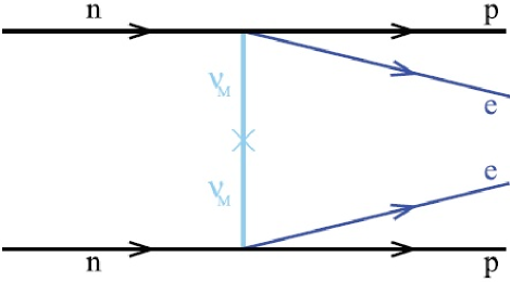
Figure 1: Feynman diagram (modified from Ref.  Engel and Menèndez, 2017) for $0\nu\beta\beta$ decay mediated by light-neutrino exchange. Two neutrons (n) decay into two protons (p), emitting two electrons ($\text{e}^{-}$). No neutrinos are emitted, implying that they are Majorana particles ($\nu_{\text{M}}$).

We consider $0\nu\beta\beta$ decay caused by the exchange of the three light Majorana neutrinos and the Standard-Model weak interaction as depicted in Fig.  (1); all contributions from other LNV processes are neglected.

Drawing on Refs.  Engel and Menèndez, 2017; Avignone et al., 2008 and the approximations employed there, we write the $0\nu\beta\beta$-decay rate as

$$\left[T_{1/2}^{0\nu}\right]^{-1}=G_{0\nu}\left(Q,Z\right)\left|M_{0\nu}\right|^{2}\left|\underset{k}{\sum}m_{k}U_{ek}^{2}\right|^{2}\,,$$ (1)

where $Q$ is the difference between initial ($i$) and final ($f$) state energies, (i.e. $Q\equiv E_{i}-E_{f}$), $Z$ is the proton number of the final nucleus, $m_{k}$ is the Majorana mass eigenvalue, and $U_{ek}$ is the element of the neutrino mixing matrix that connects the electron neutrino with mass eigenstate $k$. $G_{0\nu}\left(Q,Z\right)$ comes from the phase-space integral, which has been evaluated with improved precision in Refs.  Kotila and Iachello, 2012; Stoica and Mirea, 2013.

In this study, we focus on the ${}^{6}\text{He}\rightarrow{}^{6}\text{Be}$ ground-state-to-ground-state NME, $M_{0\nu}$ (Simkovic et al., 1999; Horoi and Stoica, 2010; Rodin et al., 2006), obtained from the $0\nu\beta\beta$-decay many-body operator, $O_{0\nu}$, as

$$M_{0\nu}=\langle^{6}\text{Be}|O_{0\nu}|^{6}\text{He}\rangle.$$ (2)

Our notation follows that of Ref. Suhonen, 2007 unless specified otherwise.

II.1 The $0\nu\beta\beta$-decay Matrix Elements

The many-body operator $O_{0\nu}$ is conventionally divided into three contributions, labeled Fermi, Gamow-Teller (GT), and tensor. We use the symbol $O$ to generically denote any one of these contributions’ corresponding two-body operator, which may always be written in second-quantized form as

$$O =\frac{1}{4}\underset{\alpha\beta\gamma\delta}{\sum}\langle\alpha\beta|O|\gamma\delta\rangle a_{\alpha}^{\dagger}a_{\beta}^{\dagger}a_{\delta}a_{\gamma}$$ (3)

where $a^{\dagger}$ and $a$ create and annihilate nucleons, respectively, in single-particle states. A given single-particle state $\alpha$ is defined by the quantum numbers $n_{\alpha}$, $l_{\alpha}$, $s_{\alpha}$, $j_{\alpha}$, $t_{\alpha}$, $m_{j\alpha}$, and $m_{t\alpha}$, which correspond to the radial, angular momentum, spin, total angular momentum, isospin, angular momentum projection, and isospin projection, respectively. Greek indices $\alpha,\beta,\gamma,\delta$ are used to denote single-particle states, while the corresponding Roman indices $a,b,c,d$ refer to the reduced set of quantum numbers, such that $a_{\alpha}^{\dagger}\equiv a_{a,m_{j\alpha},m_{t\alpha}}^{\dagger}$. We define spherical tensor/isotensor versions of the annihilation operators as

$$\hat{a}_{\delta} \equiv\left(-1\right)^{j_{\delta}+m_{j\delta}+\frac{1}{2}+m_{t\delta}}a_{d,-m_{j\delta},-m_{t\delta}}\,,$$ (4)

such that

$$a_{\delta}a_{\gamma}=\left(-1\right)^{j_{\gamma}+j_{\delta}+m_{j\gamma}+m_{j\delta}+1}\hat{a}_{c,-m_{j\gamma},-m_{t\gamma}}\hat{a}_{d,-m_{j\delta},-m_{t\delta}}\,.$$ (5)

For the ground-state-to-ground-state portion of the ${}^{6}\text{He}\rightarrow^{6}\text{Be}$ transition, we may narrow our scope to components of the two-body operators that contribute to $0^{+}\rightarrow 0^{+}$ NMEs. Expanding Eq.  (3) into doubly-reduced tensorial components in the $JT$-coupled two-body isospin representation yields for this transition

$$O_{0,-2}^{0,2} =-\frac{1}{4\sqrt{3}}\underset{abcd}{\sum}\underset{J}{\sum}\left(\mathcal{N}_{ab}\left(J,1\right)\mathcal{N}_{cd}\left(J,1\right)\right)^{-1}$$

$$\cdot(ab;J\,1|||O^{0,2}|||cd;J\,1)$$

$$\cdot\left[\left[a_{a}^{\dagger}a_{b}^{\dagger}\right]^{J,1}\left[\hat{a}_{c}\hat{a}_{d}\right]^{J,1}\right]_{0,-2}^{0,2}\,,$$ (6)

where brackets denote tensor products with tensor, isotensor couplings in superscripts and their corresponding projections in subscripts, $\mathcal{N}_{ij}(J,T)\equiv\sqrt{1-\delta_{ij}(-1)^{J+T}}/(1+\delta_{ij})$ is an antisymmetrization factor, and the triple lines ’|||’ denote doubly-reduced two-body matrix elements (TBMEs). In Eq.  (6) we implicitly include only two-body states that satisfy the Pauli exclusion principle in the sum over nucleon states (or, effectively, we only consider values of $i$, $j$, $J$, and $T$ such that $\mathcal{N}_{ij}(J,T)\neq 0$).

We express the total NME ($M_{0\nu}$) as the sum of the Fermi ($M_{0\nu}^{F}$), GT ($M_{0\nu}^{GT}$), and tensor ($M_{0\nu}^{T}$) contributions

$$M_{0\nu}=M_{0\nu}^{F}+M_{0\nu}^{GT}+M_{0\nu}^{T}\,.$$ (7)

These three NME contributions are developed for the many-body initial and final nuclear states from the doubly-reduced TBMEs of the three corresponding two-body operators. We evaluate the NMEs by summing the two-body contribution from each unique pair of the system’s nucleons. We calculate the TBMEs with the two-body operators

$$O_{0\nu}^{F}\left(r\right) =\frac{4R}{\pi g_{A}^{2}}\int_{0}^{\infty}|\mathbf{q}|d|\mathbf{q}|\frac{j_{0}(|\mathbf{q}|r)h_{F}(|\mathbf{q}|)}{|\mathbf{q}|+\bar{E}-(E_{i}+E_{f})/2}\tau_{1}^{+}\tau_{2}^{+}\,,$$

$$O_{0\nu}^{GT}\left(r\right) =\frac{4R}{\pi g_{A}^{2}}\int_{0}^{\infty}|\mathbf{q}|d|\mathbf{q}|\frac{j_{0}(|\mathbf{q}|r)h_{GT}(|\mathbf{q}|)\boldsymbol{\sigma}_{1}\cdot\boldsymbol{\sigma}_{2}}{|\mathbf{q}|+\bar{E}-(E_{i}+E_{f})/2}\tau_{1}^{+}\tau_{2}^{+}\,,$$

$$O_{0\nu}^{T}\left(r\right) =\frac{4R}{\pi g_{A}^{2}}\int_{0}^{\infty}|\mathbf{q}|d|\mathbf{q}|\frac{j_{2}(|\mathbf{q}|r)h_{T}(|\mathbf{q}|)\boldsymbol{S}_{12}}{|\mathbf{q}|+\bar{E}-(E_{i}+E_{f})/2}\tau_{1}^{+}\tau_{2}^{+}\,,$$ (8)

where $\boldsymbol{q}$ is the momentum transfer, $r=|\boldsymbol{r}_{1}-\boldsymbol{r}_{2}|$ is the magnitude of the inter-nucleon position vector, and $\hat{\boldsymbol{r}}$ is the corresponding unit vector. Additionally, $\boldsymbol{r}_{1\backslash 2}$, $\boldsymbol{\sigma}_{1\backslash 2}$, and $\tau_{1\backslash 2}^{+}$ respectively denote the labeled nucleon’s position operator, spin operator, and isospin raising operator (transforming neutrons to protons), while $\boldsymbol{S}_{12}=3\boldsymbol{\sigma}_{1}\cdot\hat{\boldsymbol{r}}\boldsymbol{\sigma}_{2}\cdot\hat{\boldsymbol{r}}-\boldsymbol{\sigma}_{1}\cdot\boldsymbol{\sigma}_{2}$ is the tensor operator. The NMEs contain $r$-dependence through the spherical Bessel functions $j_{0}$ and $j_{2}$ in Eq.  (8), and, for several heavy parent nuclei, have been shown to vanish at small distances $r$, fall off like $\nicefrac{{1}}{{r}}$ at large distance, and have a typical range of a few femtometers (fm) (Simkovic et al., 2008). Hence, we expect good convergence with the basis space for these operators in our calculations.

The neutrino potentials, $h$, are defined in momentum space as

$$h_{F}\left(|\boldsymbol{q}|\right) \equiv-g_{V}^{2}(\boldsymbol{q}^{2})\,,$$

$$h_{GT}\left(|\boldsymbol{q}|\right) \equiv g_{A}^{2}(\boldsymbol{q}^{2})-\frac{g_{A}(\boldsymbol{q}^{2})g_{P}(\boldsymbol{q}^{2})\boldsymbol{q}^{2}}{3m_{N}}+\frac{g_{P}^{2}(\boldsymbol{q}^{2})\boldsymbol{q}^{4}}{12m_{N}^{2}}+\frac{g_{M}^{2}(\boldsymbol{q}^{2})\boldsymbol{q}^{2}}{6m_{N}^{2}}\,,$$

$$h_{T}\left(|\boldsymbol{q}|\right) \equiv\frac{g_{A}(\boldsymbol{q}^{2})g_{P}(\boldsymbol{q}^{2})\boldsymbol{q}^{2}}{3m_{N}}-\frac{g_{P}^{2}(\boldsymbol{q}^{2})\boldsymbol{q}^{4}}{12m_{N}^{2}}+\frac{g_{M}^{2}(\boldsymbol{q}^{2})\boldsymbol{q}^{2}}{12m_{N}^{2}}\,,$$ (9)

where $g_{M}\left(q^{2}\right)=\left(1+\kappa_{1}\right)g_{V}\left(q^{2}\right)\simeq 4.706g_{V}\left(q^{2}\right)$ (with the anomalous nucleon isovector magnetic moment $\kappa_{1}=3.706$), and the Goldberger–Treiman relation $g_{P}\left(q^{2}\right)=2m_{N}g_{A}\left(q^{2}\right)/\left(\boldsymbol{q}^{2}+m_{\pi}^{2}\right)$ (with nucleon mass $m_{N}$ and pion mass $m_{\pi}$) connects the pseudoscalar and axial terms (Simkovic et al., 2009; Engel and Menèndez, 2017). The conservation of the vector current implies that $g_{V}\equiv\left.g_{V}\left(q^{2}\right)\right|_{0}=1$, while the value $g_{A}\equiv\left.g_{A}\left(q^{2}\right)\right|_{0}\simeq 1.27$ may be extracted from neutron $\beta$-decay measurements. Their momentum transfer dependence is $g_{V}\left(q^{2}\right)=g_{V}\left(1+q^{2}/\Lambda_{V}^{2}\right)^{-2}$ and $g_{A}\left(q^{2}\right)=g_{A}\left(1+q^{2}/\Lambda_{A}^{2}\right)^{-2}$ where $\Lambda_{V}=850$ MeV and $\Lambda_{A}=1040$ MeV are the vector and axial masses, respectively. The nuclear radius $R=1.2A^{\frac{1}{3}}\approx 2.2$ fm is inserted by convention to make the matrix elements dimensionless, with a compensating factor absorbed into $G_{0\nu}$ in Eq.  (1). Finally, $\bar{E}$ is an estimate of the average intermediate-state energy, the choice of which has been shown to have only a mild influence on the decay amplitude (Avignone et al., 2008). We employ the value $\bar{E}-(E_{i}+E_{f})/2\equiv 5\,\text{MeV}$ throughout this work.

In other prescriptions, the operators defined by Eq.  (8) are sometimes multiplied by an additional radial function, $f(r)$, designed to take into account short-range correlations that are omitted by Hilbert-space truncations performed in the many-body calculations (Miller and Spencer, 1976; Roth et al., 2005; Brueckner, 1955; Benhar et al., 2014; Muther and Polls, 2000). In this work, we assume all relevant nucleon-nucleon correlations are embedded in the many-body wavefunctions generated in our NCSM and MR-IMSRG model spaces and employ no additional radial function. We numerically integrate the inner products of the operators in Eq.  (8) using relative HO states to obtain reduced matrix elements in the relative basis. These elements are then converted to M-scheme TBMEs via a Moshinsky transformation (Tobocman, 1981; Barrett et al., 2013) before being employed in many-body calculations.

II.2 $0\nu\beta\beta$ decay in ${}^{6}\text{{He}}$ with Isospin Symmetry

When considering isovector operators, a common challenge shared by many $ab\,initio$ nuclear approaches (particularly those relying on finite matrix methods) arises when the initial and final nuclei are not the same, as the many-body spaces for the two will generally differ. In NCSM calculations, this problem usually requires the many-body eigenstate wavefunctions of the two systems to be calculated independently. In the MR-IMSRG, two different unitary transformation operators must be constructed, one for the initial nucleus and one for the final nucleus.

While solutions to this problem have been developed for the NCSM and have been implemented for the MR-IMSRG (Yao et al., 2018), a careful choice of transition can circumvent the issue when isospin conservation is a good approximation. Thus, we assume that isospin symmetry is obeyed in the mirror nuclei ⁶He and ⁶Be.

The ground states of ${}^{6}{\rm Be}$ and ${}^{6}{\rm He}$ are characterized by total angular momentum $\mathcal{J}=0$ and isospin $\mathcal{T}=1$, with projections $\mathcal{T}_{z}=-1,+1$, respectively. If isospin symmetry is obeyed, the two-body density of Eq.  (6) may be rewritten in terms of the ${}^{6}\text{He}$ two-body density alone as

$$\langle^{6}\text{Be}|\left[\left[a_{a}^{\dagger}a_{b}^{\dagger}\right]^{J,1}\left[\hat{a}_{c}\hat{a}_{d}\right]^{J,1}\right]_{0,-2}^{0,2}|^{6}\text{He}\rangle$$

$$=\sqrt{6}\langle^{6}\text{He}|\left[\left[a_{a}^{\dagger}a_{b}^{\dagger}\right]^{J,1}\left[\hat{a}_{c}\hat{a}_{d}\right]^{J,1}\right]_{0,0}^{0,2}|^{6}\text{He}\rangle.$$ (10)

III benchmarked methods

Both the NCSM and MR-IMSRG can provide accurate results when applied in light nuclei. The MR-IMSRG has the advantage that, with suitable approximations, it can be applied in heavier systems (Bogner et al., 2014; Stroberg et al., 2016, 2017). For the NCSM one may envision applications in heavier systems by merging it with renormalization approaches or by introducing an inert core and deriving effective interactions for valence-space Shell model calculations (see e.g., Refs. Jansen et al., 2014; Dikmen et al., 2015; Jansen et al., 2016; Barrett et al., 2017). The approximations involved in these envisioned approaches to heavier nuclei will also require benchmarking.

Both methods consider the $A$-body nuclear Hamiltonian, $H$, consisting of a relative kinetic-energy term and interaction terms, i.e.

$$H=\frac{1}{2Am_{N}}\underset{i<j}{\overset{A}{\sum}}\left(p_{i}-p_{j}\right)^{2}+V_{NN}+V_{NNN}+...$$ (11)

where $m_{N}$ is the average nucleon mass, $V_{NN}$ is the NN-interaction, and $p_{i}$ denotes the momentum of nucleon $i$. We follow the convention for two-body operators where summations over nucleon pairs are performed under the ordering given by $i<j$ to avoid counting the same pair twice. The term $V_{NNN}$ denotes three-body interactions, also called 3-nucleon forces (3NFs), which may be supplemented by higher-body interactions. Although studies have demonstrated that 3NFs can have a significant impact on calculated nuclear observables (Barrett et al., 2013), their inclusion would greatly increase computational cost and is thus deferred to future efforts. We therefore consider here only the NN-interactions from N3LO-EM500 (Entem and Machleidt, 2003; Machleidt and Entem, 2011), which is charge-dependent.

III.1 No-Core Shell Model

The NCSM (Barrett et al., 2013) is a configuration-interaction (CI) approach in which the many-body basis states, $|\Phi\rangle$, are expressed as Slater determinants of single-particle states occupied by the system’s nucleons, or

$$|\Phi\rangle=\mathcal{\mathcal{A}}\left[\underset{i}{\prod}|\phi_{\alpha_{i}}\rangle\right]\,,$$ (12)

where $|\phi_{\alpha_{i}}\rangle$ denotes a single-particle state with quantum numbers $\alpha_{i}$ occupied by nucleon $i$, and $\mathcal{A}$ is an antisymmetrization operator that carries both the sign permutations of the determinant and an overall normalization factor. Our NCSM approach features separate Slater determinants for the neutrons and protons, and the resulting many-body basis is specific to the nucleus under consideration. For a given application, we form total Slater determinants of fixed parity and fixed total angular momentum projection $M_{J}$.

The infinite HO basis (with energy scale fixed by the usual parameter $\hbar\Omega$) is the conventional choice of single-particle basis and is used in this work. Additional details on the HO basis functions may be found in Ref.  Barrett et al., 2013.

The nuclear many-body wavefunctions, $\Psi\left(r_{1},...,r_{A}\right)$, satisfy the A-body Schrödinger equation and are obtained by solving the Hamiltonian matrix eigenvalue problem

$$H|\Psi\rangle=E|\Psi\rangle$$ (13)

where $E$ is the eigenenergy of nuclear state $|\Psi\rangle$. Beginning with the kinetic-energy and interaction TBMEs in the HO basis, one constructs the $A$-body Hamiltonian matrix elements in the many-body basis as $\langle\Phi_{\mu}|H_{A}|\Phi_{\nu}\rangle$, where the indices $\mu$ and $\nu$ label the many-body basis states. The many-body eigenstates are then linear combinations of many-body basis states:

$$|\Psi\rangle=\underset{\mu}{\overset{\infty}{\sum}}c_{\mu}|\Phi_{\mu}\rangle$$ (14)

where $c_{\mu}$ are the normalized coefficients of the many-body basis states $|\Phi_{\mu}\rangle$. For practical calculations, the infinite many-body basis requires truncation, which one controls by using a basis cutoff parameter. For NCSM calculations performed in this study, we employ the cutoff parameter $N_{\text{max}}$, which denotes the maximum number of HO excitation quanta allowed in the many-body basis above the minimum number required by the Pauli principle (Barrett et al., 2013).

Solving Eq.  (13) with the resulting finite many-body Hamiltonian then becomes a large (but generally sparse) matrix eigenvalue problem. We obtain the solution with the hybrid OpenMP/MPI CI code Many Fermion Dynamics for nucleons (MFDn). The code is optimized for solving the large sparse matrix eigenvalue problem by using a Lanczos-like algorithm to determine the desired lowest-lying energy eigenvalues and corresponding eigenvectors. The eigenvectors are then used with other operator matrix elements to calculate that operator’s expectation values during post-processing. For more details on MFDn, see Refs.  Maris et al., 2010; Aktulga et al., 2014; Shao et al., 2017.

By solving the system in a sequence of increasingly large bases, one can extrapolate to the result when using the complete basis (i.e. when the matrix dimension of $H$ goes to infinity and the calculation becomes exact). Any other observable can also, in principle, be extrapolated to this limit, and such extrapolations are a distinguishing feature of No-Core Full-Configuration (NCFC) studies (Maris et al., 2009).

III.2 Multi-Reference In-Medium Similarity Renormalization Group

Here we provide a brief overview of the MR-IMSRG; a more complete description may be found in Refs.  Hergert et al., 2016; Hergert, 2017; Hergert et al., 2018. For an initial Hamiltonian $H$, the flow equation

$$\dfrac{dH(s)}{ds}=[\eta(s),H(s)]\,,$$ (15)

determines a unitary transformation of the Hamiltonian. Here $\eta$ is called the generator of scale transformations and $s$ is the flow parameter, defined such that $H(s)\mid_{s=0}$ is just $H$. The ground-state energy is simply given by the expectation value of the evolved Hamiltonian $H(s)$ in the reference state. Instead of solving the set of differential equations for $H(s)$ in Eq.  (7), one can solve a similar flow equation for the unitary transformation operator $U(s)$,

$$\frac{dU\left(s\right)}{ds}=\eta\left(s\right)U\left(s\right)\,,$$

whose solution can formally be written in terms of the ${\cal S}$-ordered exponential

$$U\left(s\right)=\mathcal{S}\,\text{exp}\int_{0}^{s}ds^{\prime}\eta\left(s^{\prime}\right)\,,$$ (16)

which is short-hand for the Dyson series expansion of $U(s)$. As shown first by Magnus, it is possible to rewrite the unitary transformation operator as $U(s)\equiv e^{\Omega(s)}$, a step that transforms the equation for $U(s)$ into one for $\Omega$ (Morris et al., 2015):

$$\frac{d\Omega\left(s\right)}{ds}=\underset{n=0}{\overset{\infty}{\sum}}\frac{B_{n}}{n!}\left[\Omega\left(s\right),\eta\left(s\right)\right]^{\left(n\right)}\,.$$ (17)

The nested commutators in this equation are given by

$$\left[\Omega\left(s\right),\eta\left(s\right)\right]^{\left(0\right)} =\eta\left(s\right)\,,$$ (18a)

$$\left[\Omega\left(s\right),\eta\left(s\right)\right]^{\left(n\right)} =\left[\Omega\left(s\right),\left[\Omega\left(s\right),\eta\left(s\right)\right]^{\left(n-1\right)}\right]\,,$$ (18b)

and $B_{n=0,1,2,\cdots}$ are the Bernoulli numbers $\{1,-1/2,1/6,\cdots\}$.

The expectation value of any operator $O$ is then given by $\langle\Phi|O\left(s\right)|\Phi\rangle=\langle\Phi|e^{\Omega(s)}O{}^{-\Omega(s)}|\Phi\rangle$, and can be evaluated with the Baker-Campbell-Hausdorff formula:

$$e^{\Omega(s)}Oe^{-\Omega(s)}=\underset{n=0}{\overset{\infty}{\sum}}\frac{1}{n!}\left[\Omega\left(s\right),O\right]^{\left(n\right)}.$$ (19)

In the MR-IMSRG calculations performed here, we express all operators in normal-ordered form with respect to a reference state $|\Phi\rangle$ in order to control the proliferation of induced terms. We keep up to normal-ordered two-body operators throughout the calculation, in accordance with the MR-IMSRG(2) truncation described in Ref.  Hergert et al., 2018. We use particle-number-projected HFB quasiparticle vacua as reference states, and adopt the Brillouin generator (Hergert, 2017). We numerically solve the flow equation for values of $s$ large enough so that the solutions are very close to their asymptotic limits. The underlying Hamiltonian that defines both the projected HFB reference state and the starting point for the flow equation is determined by using the same TBMEs in the single-particle HO basis that are used in our NCSM calculations. However, unlike the NCSM, the MR-IMSRG is formulated in the natural orbital basis of the reference state. Since the reference state results from a projected HFB calculation in a HO basis, the MR-IMSRG effectively explores a configuration space controlled by the cutoff parameter $e_{\text{max}}$, which denotes the maximum number of energy quanta that the HO components of any natural orbital can have. In effect, for a given cutoff $e_{\text{max}}$, the MR-IMSRG many-body basis will include single-particle excitations up to $e_{\text{max}}$ (i.e. one-particle-one-hole, or 1p1h), two-particle excitations (i.e. 1p1h+1p1h or 2p2h) up to $2e_{\text{max}}$, uncorrelated three-body excitations (i.e. 1p1h + 1p1h + 1p1h or 1p1h + 2p2h) up to $3e_{\text{max}}$, and so on.

IV results and discussion

Here we discuss the results of the NCSM and MR-IMSRG calculations. We provide graphical representations of the results, as functions of the basis cutoff parameters, to analyze the convergence of the operators at the chosen basis scale of $\hbar\Omega=20$ MeV. Throughout, we use solid dots to represent NCSM results and open boxes to represent MR-IMSRG results. Similarly, we use solid lines to denote extrapolations of the NCSM results and dashed lines to denote extrapolations of the MR-IMSRG results.

In order to compare the convergence behavior of results from the NCSM and MR-IMSRG, we must consider the differences in their truncation schemes. We recall that the NCSM’s cutoff parameter $N_{\text{max}}$ denotes the total number of allowed $excitation$ quanta in the system, and $e_{\text{max}}$ denotes the maximum number of allowed energy quanta possessed by any single nucleon. Since in ${}^{6}\text{He }$ at a given $N_{\text{max}}$ the highest number of quanta possessed by any single-particle state will be $N_{\text{max}}+1$, we equate the two cutoffs with the assignment $e_{\text{max}}\equiv N_{\text{max}}+1$ for our comparison. While this assignment is not exact, it ensures that for a given pair of matched cutoffs, we use identical single-particle bases under both truncation schemes. Moreover, our use of this assignment to compare the results does not preclude their examination from other perspectives. Instead, we merely offer this assignment as a reasonable vehicle to present our results graphically.

We extrapolate our results to obtain predictions of observables at the continuum limit and to better examine their convergence behavior; the functional forms and other details of these extrapolations are provided in the appendix. We extrapolate our NCSM and MR-IMSRG results for energy and square radii with formulae (Eq.  (21) and Eq.  (22), respectively) inspired by those provided in Refs.  Furnstahl et al., 2012; Maris et al., 2009. Although these extrapolations were originally designed with the $N_{\text{max}}$ truncation scheme in mind, there is good reason from a theoretical perspective to expect that the same extrapolation forms effective for the NCSM will be effective for the results of IMSRG calculations (Hergert et al., 2016). Meanwhile, as is the case for many nonscalar operator observables (with the exception of those in significant investigations on extrapolating E2 observables (Odell et al., 2016)), precision extrapolation approaches for $0\nu\beta\beta$-decay observables remain largely unexplored. Guided by the similarities of the observable’s $r$-dependence seen in Ref. (Simkovic et al., 2008) to that of nuclear interactions, we employ the same simple exponential form applied for the energy to extrapolate the $0\nu\beta\beta$-decay contributions. While we acknowledge that a thorough investigation of extrapolating $0\nu\beta\beta$-decay NMEs is warranted for refined predictions and accurate uncertainty estimates, we find that this form provides an adequate fit and proves sufficient for this comparative study.

To facilitate our discussion of convergence, we refer to the speed (with respect to the cutoff parameter) at which an eigenvalue result approaches its asymptotic value as the result’s “convergence rate”. We gauge the convergence rate with the value of $N_{\text{max}}$ ($e_{\text{max}}$) at which the extrapolation is within $5\%$ of its value at the continuum limit, and denote this generally non-integer value $\widetilde{N}_{5\%}$ ($\widetilde{e}_{5\%}$). Though this metric relies heavily on the validity of the extrapolation, it provides a functional estimate for both the relative convergence speeds between results and the cutoffs required for reaching well-converged values.

Finally, in the interest of understanding what the differences between the extrapolated results of the two $ab\,initio$ calculations signify, we briefly consider the general $A$-body system. For such a system, the untruncated MR-IMSRG calculation would include all many-body correlations, and would therefore provide identical results (within numerical noise) as the NCSM at the continuum limit. By performing only the MR-IMSRG(2) calculation, we expect the two approaches’ results to converge to different values that depend on how significant the neglected three-body (up to $A$-body) correlations are to the observable in question. Thus, beyond the mild uncertainty introduced by the extrapolation, differences between the extrapolated results estimate the significance of many-body correlations neglected by the MR-IMSRG(2) calculation.

IV.1 Ground-State Energy and Nuclear Square Radius

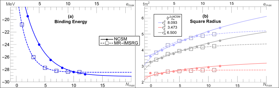
Figure 2: Ground-State energy (a) and neutron (light blue), proton (light red), and matter (gray) square radii ($r_{n}^{2}$, $r_{p}^{2}$, and $r_{m}^{2}$ respectively) (b) of ${}^{6}\text{He}$ with varying basis cutoff parameter from NCSM (solid circle) and MR-IMSRG(2) (open square) ab initio calculations. Solid and dashed lines denote the NCSM and MR-IMSRG extrapolations, respectively. The realistic N3LO-EM500 potential with energy scale $\hbar\Omega=20$ MeV and SRG evolution scale $\lambda=2.0$ $\text{fm}^{-1}$ is used in all cases. The asymptotic fit parameter, $\langle r^{2}\rangle_{\infty}$, of the NCSM square radius extrapolations are listed in the legend of (b) (see Eq.  (22) for extrapolation definition). Fit parameters and plotted values are listed in Table  (1) for energy, and in Table  (2) for the square radii.

The initial system is the ${}^{6}\text{He}$ nucleus in its ground state. The calculated ground-state energy and neutron, proton, and matter square radii ($r_{n}^{2}$, $r_{p}^{2}$, and $r_{m}^{2}$ respectively) varying with basis truncation are shown in panels (a) and (b) of Fig.  (2) respectively.

The NCSM ground-state energy extrapolation has converged to within $5\%$ of its asymptotic value of -29.132 MeV by $\widetilde{N}_{5\%}\sim 7.9$. The MR-IMSRG(2) extrapolated energy converges somewhat faster by comparison, with $\widetilde{e}_{5\%}\sim 4.9$ and the asymptotic value of -28.472 MeV (around 2.3% higher than the NCSM result). Both extrapolated ground-state energies are underbound compared to the experimental result of -29.272 MeV (Riisager et al., 1990), as well as the extrapolated results of -30.0(1) MeV and -29.87 MeV from two similar (but independent) NCFC calculations of the ${}^{6}\text{He}$ ground-state (Bogner et al., 2008; Furnstahl et al., 2012) that used only the charge-independent parts of our strong-interaction Hamiltonian.

Performing the same calculations for ${}^{4}\text{He}$ yields extrapolated binding energies of 28.305 and 28.316 MeV for the NCSM and MR-IMSRG(2), respectively. Subtracted from our ${}^{6}\text{He}$ binding energy results, this corresponds to 2$n$-separation energies of 0.827 MeV and 0.156 MeV. The experimental 2n-separation energy of ${}^{6}\text{He}$, by comparison, is approximately 0.975 MeV (Wang et al., 2017). The difference between these results is most likely a consequence of the truncations inherent to the MR-IMSRG(2). While the method probes a larger space of 2p2h excitations than the NCSM for a given pair of matched $N_{\text{max}}$ and $e_{\text{max}}$ single-particle bases, the MR-IMSRG(2) misses correlation energy from 3p3h and higher excitations that are included in the NCSM. We expect such correlations to play a more important role in a nucleus with a complex structure, like ${}^{6}\text{He}$, than in a compact nucleus like ${}^{4}\text{He}$. We will analyze this issue in more detail using improved MR-IMSRG truncations (Hergert et al., 2018) in the future.

Comparing the convergence rates of the square radii results between approaches, we see the MR-IMSRG(2) (NCSM) square radii consistently converge faster (slower), with $\widetilde{e}_{5\%}\sim 14,\,3.5,\,12$ ($\widetilde{N}_{5\%}\sim 72,\,30,\,63$) for neutron, proton, and matter square radii, respectively. This large difference in convergence speed primarily results from the use of natural orbitals in the MR-IMSRG. However, we observe the MR-IMSRG(2) results converge to a roughly $34\%,$ $21\%,$ and $31\%$ smaller value than the NCSM results for the corresponding square radii. All radii share the slower convergence rate relative to the ground-state energy that is commonly associated with the $r^{2}$ operator; a consequence of coming from an effective operator with sensitivity to correlations outside the characteristic length scale of the chosen HO basis (Barrett et al., 2013; Cockrell et al., 2012; Furnstahl et al., 2014, 2015; Coon et al., 2012). In the NCSM (and to a lesser degree MR-IMSRG), the slow convergence reflects the basis regularization of the infrared (IR) momentum region from the HO basis truncation. In effect, because the basis’s length scale is chosen to favor convergence in energy, the basis requires higher cutoffs to fully capture the longer-range correlations of the $r^{2}$ operator. The significantly faster convergence speed of the proton square radius (compared to those of the neutron and matter square radii) is a consequence of this effect, as the protons predominantly remain in the core of the ⁶He ground-state halo structure (Riisager, 2013). That is, since the protons are only found in the four-nucleon core, the proton square radius operator correlations primarily exist at the shorter distances pertinent to the core, and are thus better encompassed by the scales of the chosen basis.

The benefit of the MR-IMSRG’s renormalization can be seen in the improved convergence observed in its results. In essence, the renormalization decouples the NN-correlations existing outside the scales encompassed by the basis, and distributes those correlations inside those scales. The drawback is that some induced many-body forces must be neglected in the process, an approximation that would explain the notable differences seen in the extrapolated square radii. In the case of a light nucleus such as ${}^{6}\text{He}$ where a convergence trend can be established, we expect the NCSM extrapolated radii to be more accurate than those of the MR-IMSRG(2) for the given potential. Consequently, we conjecture that the smaller MR-IMSRG(2) square radii reflect meaningful induced many-body correlations that are being lost through the MR-IMSRG(2) many-body truncation. Specifically, the fast convergence of the MR-IMSRG(2) results suggests that the 1p1h and 2p2h correlations relevant to $r^{2}$ are well-accounted for by $e_{\text{max}}=12$ and 24, respectively, and that the remaining differences with the NCSM results are from higher many-body correlations omitted by the MR-IMSRG(2) approach.

IV.2 $0\nu\beta\beta$-decay Matrix Element

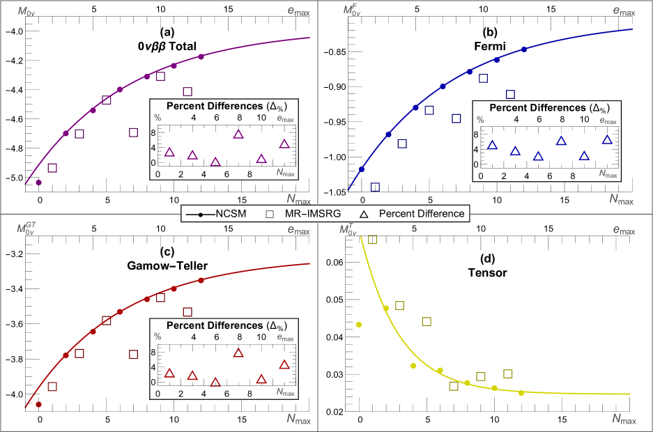
Figure 3: Ground-state-to-ground-state $0\nu\beta\beta$-decay NME (a) for ${}^{6}\text{He}\rightarrow{}^{6}\text{Be}$ , decomposed into its Fermi (b), GT (c), and tensor (d) contributions, as a function of the basis cutoff for NCSM (solid circle) and MR-IMSRG(2) (open square) ab initio calculations. Solid lines denote NCSM extrapolations. Each vertical axis is expanded for visibility. The three contributions add to the total as specified by Eq.  (7)). Insets provide the percent difference in magnitude (open triangles) between the MR-IMSRG results and the NCSM extrapolation as described in the text. Plotted values and fit parameters are listed in Table  (1).

We turn finally to the ground-state-to-ground-state ${}^{6}\text{He}\rightarrow{}^{6}\text{Be}$ $0\nu\beta\beta$-decay NME. As already mentioned, we assume isospin symmetry so that the initial and final state are described by the same wavefunction (except for an interchange of protons and neutrons). We present our results in Fig.  (3), where we recall that discrete points represent results of many-body calculations while lines represent fits specified by Eq.  (21). We decompose the total NME in (a) into its Fermi, GT, and tensor contributions from Eq.  (7) in panels (b), (c) and (d), respectively. Insets provide estimates for the percent difference, $\Delta_{\%}$, between results of the two methods within our mapping of their basis truncation schemes (we omit such estimates for the numerically less significant tensor contribution). For a given $e_{\text{max}}$, we calculate these values as

$$\left(\Delta_{\%}\right)_{e_{\text{max}}}=200\left|\frac{\left(M_{0\nu}^{\text{IMSRG}}\right)_{e_{\text{max}}}-f\left(\left[N_{\text{max}}\right]_{e_{\text{max}}}\right)}{\left(M_{0\nu}^{\text{IMSRG}}\right)_{e_{\text{max}}}+f\left(\left[N_{\text{max}}\right]_{e_{\text{max}}}\right)}\right|\,,$$ (20)

where $\left(M_{0\nu}^{\text{IMSRG}}\right)_{e_{\text{max}}}$ is the NME result of the MR-IMSRG(2) calculation with cutoff $e_{\text{max}}$, and $f\left(N_{\text{max}}\right)$ is the NCSM fit described by Eq.  (21) evaluated at the mapped cutoff value $\left[N_{\text{max}}\right]_{e_{\text{max}}}=e_{\text{max}}-1$ (visualized in the figure by the intersection of a vertical line between each open square and the NCSM extrapolation). While, much like the mapping between cutoffs, these estimates require some level of arbitration, we nevertheless find them a reasonable and useful tool for gauging the differences between methods.

The $0\nu\beta\beta$-decay NMEs from the NCSM and MR-IMSRG approaches agree remarkably well. Although the results of the MR-IMSRG(2) calculations reflect significantly larger fluctuations with each step in the basis cutoff, those fluctuations consistently remain less than a few percent of the converged value, and the overall trends remain quite similar to those of the NCSM. More importantly, the contributions, especially the larger Fermi and GT contributions, show excellent agreement between approaches.

The relative magnitudes of the contributions agree between approaches. The GT contribution is around four times greater than the Fermi contribution, while the tensor contribution is roughly two orders of magnitude smaller and of opposite sign. The Fermi, GT, tensor, and total NME results have $\widetilde{N}_{5\%}\sim 12.6,\,10.8,\,10.3,\,11.7$, respectively, which suggests only slightly slower convergence than that of the energy but still significantly faster convergence than that of the NCSM square radii.

The MR-IMSRG $0\nu\beta\beta$-decay results resemble a saw-tooth pattern for results beyond $e_{\text{max}}=4$ that gradually decreases in magnitude as $e_{\text{max}}$ increases. The maximum deviation of this pattern occurs in the GT contribution and reaches the order of a few percent. The deviations of the tensor contribution appear less systematic, though this may be a consequence of the contribution’s relatively small magnitude. The deviations in the Fermi and GT results of the MR-IMSRG share a sign and are most visible at $e_{\text{max}}=8$, where they consistently deviate in the negative direction.

A mildly similar (though less pronounced) saw-tooth pattern is observed in the tensor contribution of the NCSM results at the lowest $N_{\text{max}}$ cutoffs. Within NCSM calculations, such patterns (sometimes called “odd-even effects”) are generally the consequence of alternating signs in the asymptotic tails of the HO basis wavefunctions that are introduced with each increment in $N_{\text{max}}$ (Vary et al., 2018). In such cases, as the tail region of the calculated wavefunction shifts with each increment, the tail begins to overlap a region of phase space in which the effective operator is particularly active (i.e., has dominant correlations). If the span of that active region is long enough to require multiple steps in $N_{\text{max}}$ for the tail to pass through, the result is a visible contribution to the observable that alternates in sign. Naturally, the pattern disappears as $N_{\text{max}}$ increases enough so that the effective operator’s range is completely encompassed by that of the basis.

One might wonder if the pattern observed in the MR-IMSRG $0\nu\beta\beta$-decay results reflect a similar effect. However, considering our MR-IMSRG(2) calculations employ natural orbitals and not HO wavefunctions, the pattern’s similarity may be entirely circumstantial. Determining the origin of these deviations in the MR-IMSRG results will require further study.

Despite these fluctuations making it somewhat challenging to make more than qualitative observations, the trends of the NCSM and MR-IMSRG results are remarkably similar. Indeed, the differences in the asymptotic limits of the square radii in Fig.  (2) do not appear indicative of similar differences in the $0\nu\beta\beta$-decay NME results. Similarly however, the more rapid convergence observed in the MR-IMSRG(2) ground-state energy and square radii compared to that of the NCSM does not appear to translate into a more rapid convergence of the $0\nu\beta\beta$-decay NMEs in Fig.  (3). The differences between the two approaches’ $0\nu\beta\beta$-decay results appear to be of similar magnitudes as the saw-tooth deviations present in the MR-IMSRG(2) results, and remain less than $5\%$ of the total $0\nu\beta\beta$-decay NME at the maximum basis cutoff employed for each method.

Comparing our extrapolated $0\nu\beta\beta$-decay NMEs to those calculated in the VMC approach with 3N correlations included (Pastore et al., 2018), we see that the magnitudes of both the GT and Fermi contributions agree to within about $15\%$, while those of the tensor contribution agree to within about $10\%$. For all three contributions, the VMC results are larger. These differences may suggest a modest correction from 3N correlations, though other differences between our study and that of Ref.  Pastore et al., 2018 may play a significant role as well.

V conclusion

We find significant agreement between the NCSM and MR-IMSRG results in our investigation of $0\nu\beta\beta$ decay in the $A=6$ system. The difference in the calculated ground-state energy is only about $\sim 2.3\%$. We see measurable differences in the square-radius results that offer an estimate for the effects of correlations that are omitted by the MR-IMSRG(2) truncation at the normal-ordered two-body level. It is interesting that these differences do not extend to the $0\nu\beta\beta$-decay NMEs, which are remarkably similar in the two approaches, differing by only $\sim 4.3\%$ in the total NME at the largest basis cutoffs considered. The convergence rate of the $0\nu\beta\beta$-decay NMEs appears to be comparable to that of the energies.

The GT contribution dominates the $0\nu\beta\beta$-decay NME, comprising $\sim 80\%$ of its total. The Fermi contribution makes up most of the remainder, and the tensor contribution is roughly two orders of magnitude smaller and of opposite sign.

Our estimates of the differences in the total $0\nu\beta\beta$-decay NME between the two approaches do not exceed $9\%$ for any of the basis cutoffs considered. Fluctuations in the MR-IMSRG results could pose a minor obstacle for extrapolation, though their consistent saw-tooth appearance may suggest these fluctuations are systematically correctable. Beyond these fluctuations, the two approaches result in qualitatively similar convergence for the $0\nu\beta\beta$-decay NME.

The agreement between the two approaches for $0\nu\beta\beta$-decay NMEs is encouraging, and warrants additional benchmarking. Unlike the transition studied in this work, the physically realistic $0\nu\beta\beta$-decay transition contributions do not possess a uniform sign as a function of the pair separation (Wang et al., 2019). That is, the $(0+,T)\rightarrow(0+,T-2)$ transitions of experimental interest (Gilliss et al., 2018; Gando et al., 2016; Agostini et al., 2017) have a node in the transition density, making them much more sensitive to both short- and long-range correlations in the wavefunctions. This sensitivity has been recently explored in another benchmark study comparing VMC and shell-model calculations of $0\nu\beta\beta$ decay in $A=10$ and $A=12$ systems, and has been seen to generate differences ranging anywhere from $30\%$ to $400\%$ between approaches (Wang et al., 2019). A similar comparison between the MR-IMSRG and NCSM approaches, including full isospin dependence, would provide a more stringent test of the many-body methods, and greater insight into problems that may appear when modeling the decay in heavier nuclei. The results observed here warrant such an investigation, and lend support to the application of MR-IMSRG to $0\nu\beta\beta$ decay in heavier nuclei (Yao et al., 2019), where it is computationally more feasible than the NCSM. The good agreement between the two approaches for $0\nu\beta\beta$-decay NMEs is a promising development.

appendix: extrapolation methods

In this work, we perform all extrapolations by using a non-linear least-squares fit to a form that is specific to each observable and varies with cutoff parameter. The fitting process is iterated until all fit parameters have converged to at least 10 digits of precision. We apply forms identically for both NCSM and MR-IMSRG extrapolations, treating the former as functions of $N_{\text{max}}$ and the latter as functions of $e_{\text{max}}$. We use $X_{\text{max}}$ to denote either cutoff parameter when defining the extrapolations provided below. Following a common NCFC practice, we do not include the $N_{\text{max}}=0$ result when performing fits to any of the NCSM data sets. The extrapolation for each data set is performed without regard to any other data sets or their extrapolations. The formulae for ground-state energy and square radius are applied identically to both NCSM and MR-IMSRG results. Extrapolations for $0\nu\beta\beta$-decay NMEs are only performed for the NCSM results because of fluctuations in the MR-IMSRG results.

It should be noted that the extrapolations described here were originally designed with the $N_{\text{max}}$ truncation scheme in mind, and their effectiveness for extrapolating results in the $e_{\text{max}}$ truncation scheme has not yet been fully explored. Nevertheless, the significant similarities of the two schemes and their quantification of the same underlying variable (i.e. the content of the many-body basis) suggest the same extrapolation forms may be effective; an expectation that is supported by the results of this work.

Motivated by the extrapolations proposed in Ref.  Maris et al., 2009, we extrapolate the ground-state energy to the form

$$f\left(X_{\text{max}}\right) =a+b\cdot e^{-cX_{\text{max}}}$$ (21)

where $a$, $b$, and $c$ are fit parameters. We employ the same form for our extrapolations of the NCSM $0\nu\beta\beta$-decay results. Values of fit parameters calculated in this study for energy and $0\nu\beta\beta$-decay NMEs may be found in the right-most columns of Table  (1) alongside their corresponding data set.

The simple exponential form depicted in Eq.  (21) generally provides a poor prediction for the convergence behavior of square-radius operator observables. Thus, inspired by the methods discussed in Ref.  Furnstahl et al., 2012, we extrapolate square radii by fitting to the form

$$\langle r^{2}\rangle =\langle r^{2}\rangle_{\infty}-\left(c_{0}\beta+c_{1}\beta^{3}\right)e^{-\beta}\,,$$ (22)

where

$$\beta\equiv 2k_{\infty}\frac{\hbar}{m\Omega}\left[\sqrt{2X_{\text{max}}+5}+0.54437\left(2X_{\text{max}}+5\right)^{1/6}\right]\,.$$

Here $m=938.92$ MeV is the average mass of a neutron and a proton, and $\langle r^{2}\rangle_{\infty},$ $c_{0}$, and $c_{1}$ are fit parameters. Unlike the authors of Ref.  Furnstahl et al., 2012 who determine $k_{\infty}$ while extrapolating the ground-state energy with their theoretically-founded “IR formula”, we treat $k_{\infty}$ as an additional fit parameter when extrapolating each square radius. We provide our calculated values of the fit parameters for each square radius extrapolation alongside its corresponding data set in Table  (2).

Table 1: MR-IMSRG(2) and NCSM calculated observables and extrapolation parameters (see Eq.  (21)). The ground-state energy ($E$) results correspond to the ${}^{6}\text{He}$ ground state, and are plotted in Fig.  (2). The $0\nu\beta\beta$-decay NME ($M_{0\nu}$) results and their decomposition into Fermi (F), Gamow-Teller (GT), and tensor (T) contributions correspond to the${}^{6}\text{He}\rightarrow{}^{6}\text{Be}$ ground-state-to-ground-state transition, and are plotted in Fig.  (3). In all calculations of $M_{0\nu}$ and its contributions, isospin symmetry has been assumed. Extrapolations for the $0\nu\beta\beta$-decay NME were only performed using the NCSM results.

		$N_{\text{max}}$($e_{\text{max}}$)							Fit Parameters
Observable	Method	0(2)	2(4)	4(6)	6(8)	8(10)	10(12)	12	$a$	$b$	$c$
$E$ (MeV)	NCSM	-12.546	-19.406	-23.961	-26.438	-27.699	-28.374	-28.720	-29.132	18.414	0.3188
	MR-IMSRG	-20.810	-26.037	-27.752	-28.240	-28.385	-28.435		-28.472	24.375	0.5784
$M_{0\nu}^{F}$	NCSM	-1.0165	-0.9669	-0.9287	-0.8984	-0.8773	-0.8604	-0.8458	-0.8032	-0.2135	0.1331
	MR-IMSRG	-1.0430	-0.9811	-0.9335	-0.9452	-0.8880	-0.9110
$M_{0\nu}^{GT}$	NCSM	-4.0553	-3.7751	-3.6398	-3.5256	-3.4546	-3.3960	-3.3471	-3.2144	-0.7472	0.1429
	MR-IMSRG	-3.9576	-3.7688	-3.5812	-3.7742	-3.4503	-3.5326
$M_{0\nu}^{T}$	NCSM	0.0435	0.0479	0.0325	0.0313	0.0279	0.0265	0.0252	0.0247	0.0441	0.3472
	MR-IMSRG	0.0661	0.0484	0.0441	0.0268	0.0294	0.0301
$M_{0\nu}$	NCSM	-5.0283	-4.6941	-4.5361	-4.3926	-4.3041	-4.2299	-4.1677	-3.9777	-0.9355	0.1322
	MR-IMSRG	-4.9346	-4.7016	-4.4706	-4.6927	-4.3089	-4.4134

Table 2: MR-IMSRG(2) and NCSM neutron, proton, and matter square radii ($r_{n}^{2}$, $r_{p}^{2}$, and $r_{m}^{2}$, respectively) and corresponding square radius extrapolation parameters (see Eq.  (22)) for the ${}^{6}\text{He}$ ground state. The extrapolated fits are plotted alongside their respective results in Fig.  (2).

		$N_{\text{max}}$($e_{\text{max}}$)							Fit Parameters
Observable	Method	0(2)	2(4)	4(6)	6(8)	8(10)	10(12)	12	$\langle r^{2}\rangle_{\infty}$	$c_{0}$	$c_{1}$	$k_{\infty}$
$r_{n}^{2}$ ($\text{fm}^{2}$)	NCSM	3.6286	4.0096	4.3347	4.6604	4.9169	5.1656	5.4014	8.0927	10.9067	0.9965	0.1238
	MR-IMSRG	3.8389	4.3023	4.5616	4.7524	4.8929	4.9903		5.3226	10.601	0.2827	0.2235
$r_{p}^{2}$ ($\text{fm}^{2}$)	NCSM	2.5918	2.5622	2.6955	2.8056	2.8791	2.9532	3.0217	3.4732	3.0146	0.1924	0.1505
	MR-IMSRG	2.5125	2.6540	2.6870	2.7149	2.7394	2.7543		2.7598	8.9888	0.0807	0.3546
$r_{m}^{2}$ ($\text{fm}^{2}$)	NCSM	3.2830	3.5273	3.7885	4.0421	4.2378	4.4285	4.6083	6.5005	8.1034	0.7285	0.1282
	MR-IMSRG	3.3970	3.7527	3.9367	4.0733	4.1751	4.2448		4.4563	8.4272	0.2028	0.2326

References

- Ahmad et al. (2001) Q. R. Ahmad et al. (SNO), Phys. Rev. Lett. 87, 071301 (2001), arXiv:nucl-ex/0106015 [nucl-ex] .
- Eguchi et al. (2003) K. Eguchi et al. (KamLAND), Phys. Rev. Lett. 90, 021802 (2003), arXiv:hep-ex/0212021 [hep-ex] .
- Fukuda et al. (1998) Y. Fukuda et al. (Super-Kamiokande), Phys. Rev. Lett. 81, 1562 (1998), arXiv:hep-ex/9807003 [hep-ex] .
- Martin-Albo et al. (2016) J. Martin-Albo et al. (NEXT), JHEP 05, 159 (2016), arXiv:1511.09246 [physics.ins-det] .
- Albert et al. (2014) J. B. Albert et al. (EXO-200), Nature 510, 229 (2014), arXiv:1402.6956 [nucl-ex] .
- Gilliss et al. (2018) T. Gilliss et al. (MAJORANA), Proceedings, 21st International Conference on Particles and Nuclei (PANIC 17): Beijing, China, September 1-5, 2017, Int. J. Mod. Phys. Conf. Ser. 46, 1860049 (2018), arXiv:1804.01582 [physics.ins-det] .
- Gando et al. (2016) A. Gando, Y. Gando, T. Hachiya, A. Hayashi, S. Hayashida, H. Ikeda, K. Inoue, K. Ishidoshiro, Y. Karino, et al. (KamLAND-Zen), Phys. Rev. Lett. 117, 082503 (2016), [Addendum: Phys. Rev. Lett.117,no.10,109903(2016)], arXiv:1605.02889 [hep-ex] .
- Alfonso et al. (2015) K. Alfonso et al. (CUORE), Phys. Rev. Lett. 115, 102502 (2015), arXiv:1504.02454 [nucl-ex] .
- Agostini et al. (2017) M. Agostini et al., (2017), 10.1038/nature21717, [Nature544,47(2017)], arXiv:1703.00570 [nucl-ex] .
- Aalseth et al. (2018) C. E. Aalseth et al. (Majorana), Phys. Rev. Lett. 120, 132502 (2018), arXiv:1710.11608 [nucl-ex] .
- Andringa et al. (2016) S. Andringa et al. (SNO+), Adv. High Energy Phys. 2016, 6194250 (2016), arXiv:1508.05759 [physics.ins-det] .
- Iwata et al. (2016) Y. Iwata, N. Shimizu, T. Otsuka, Y. Utsuno, J. Menèndez, M. Honma, and T. Abe, Phys. Rev. Lett. 116, 112502 (2016), [Erratum: Phys. Rev. Lett.117,no.17,179902(2016)], arXiv:1602.07822 [nucl-th] .
- Cirigliano et al. (2017) V. Cirigliano, W. Dekens, J. de Vries, M. L. Graesser, and E. Mereghetti, JHEP 12, 082 (2017), arXiv:1708.09390 [hep-ph] .
- Contessi et al. (2017) L. Contessi, A. Lovato, F. Pederiva, A. Roggero, J. Kirscher, and U. van Kolck, Phys. Lett. B772, 839 (2017), arXiv:1701.06516 [nucl-th] .
- Coraggio et al. (2017) L. Coraggio, L. De Angelis, T. Fukui, A. Gargano, and N. Itaco, Phys. Rev. C95, 064324 (2017), arXiv:1703.05087 [nucl-th] .
- Jiao et al. (2017) C. F. Jiao, J. Engel, and J. D. Holt, Phys. Rev. C96, 054310 (2017), arXiv:1707.03940 [nucl-th] .
- Tiburzi et al. (2017) B. C. Tiburzi, M. L. Wagman, F. Winter, E. Chang, Z. Davoudi, W. Detmold, K. Orginos, M. J. Savage, and P. E. Shanahan, Phys. Rev. D96, 054505 (2017), arXiv:1702.02929 [hep-lat] .
- Shanahan et al. (2017) P. E. Shanahan, B. C. Tiburzi, M. L. Wagman, F. Winter, E. Chang, Z. Davoudi, W. Detmold, K. Orginos, and M. J. Savage, Phys. Rev. Lett. 119, 062003 (2017), arXiv:1701.03456 [hep-lat] .
- Horoi and Neacsu (2017) M. Horoi and A. Neacsu, (2017), arXiv:1706.05391 [hep-ph] .
- Cremonesi and Pavan (2014) O. Cremonesi and M. Pavan, Adv. High Energy Phys. 2014, 951432 (2014), arXiv:1310.4692 [physics.ins-det] .
- Dell’Oro et al. (2016) S. Dell’Oro, S. Marcocci, M. Viel, and F. Vissani, Adv. High Energy Phys. 2016, 2162659 (2016), arXiv:1601.07512 [hep-ph] .
- Engel and Menèndez (2017) J. Engel and J. Menèndez, Rept. Prog. Phys. 80, 046301 (2017), arXiv:1610.06548 [nucl-th] .
- Gomez-Cadenas et al. (2012) J. J. Gomez-Cadenas, J. Martin-Albo, M. Mezzetto, F. Monrabal, and M. Sorel, Riv. Nuovo Cim. 35, 29 (2012), arXiv:1109.5515 [hep-ex] .
- Henning (2016) R. Henning, Rev. Phys. 1, 29 (2016).
- Gysbers et al. (2019) P. Gysbers et al., Nature Phys. 15, 428 (2019), arXiv:1903.00047 [nucl-th] .
- Bogner et al. (2014) S. K. Bogner, H. Hergert, J. D. Holt, A. Schwenk, S. Binder, A. Calci, J. Langhammer, and R. Roth, Phys. Rev. Lett. 113, 142501 (2014), arXiv:1402.1407 [nucl-th] .
- Jansen et al. (2014) G. R. Jansen, J. Engel, G. Hagen, P. Navràtil, and A. Signoracci, Phys. Rev. Lett. 113, 142502 (2014), arXiv:1402.2563 [nucl-th] .
- Jansen et al. (2016) G. R. Jansen, M. D. Schuster, A. Signoracci, G. Hagen, and P. Navràtil, Phys. Rev. C94, 011301(R) (2016), arXiv:1511.00757 [nucl-th] .
- Stroberg et al. (2016) S. R. Stroberg, H. Hergert, J. D. Holt, S. K. Bogner, and A. Schwenk, Phys. Rev. C93, 051301(R) (2016), arXiv:1511.02802 [nucl-th] .
- Stroberg et al. (2017) S. R. Stroberg, A. Calci, H. Hergert, J. D. Holt, S. K. Bogner, R. Roth, and A. Schwenk, Phys. Rev. Lett. 118, 032502 (2017), arXiv:1607.03229 [nucl-th] .
- Dikmen et al. (2015) E. Dikmen, A. F. Lisetskiy, B. R. Barrett, P. Maris, A. M. Shirokov, and J. P. Vary, Phys. Rev. C91, 064301 (2015), arXiv:1502.00700 [nucl-th] .
- Barrett et al. (2017) B. R. Barrett, E. Dikmen, P. Maris, A. M. Shirokov, N. A. Smirnova, and J. P. Vary, Proceedings, 14th International Symposium on Nuclei in the Cosmos (NIC-XIV): Niigata, Japan, June 19-24, 2016, JPS Conf. Proc. 14, 021006 (2017).
- Song et al. (2017) L. S. Song, J. M. Yao, P. Ring, and J. Meng, Phys. Rev. C95, 024305 (2017), arXiv:1702.02448 [nucl-th] .
- Yao et al. (2018) J. M. Yao, J. Engel, L. J. Wang, C. F. Jiao, and H. Hergert, Phys. Rev. C98, 054311 (2018), arXiv:1807.11053 [nucl-th] .
- Entem and Machleidt (2003) D. R. Entem and R. Machleidt, Phys. Rev. C68, 041001(R) (2003), arXiv:nucl-th/0304018 [nucl-th] .
- Machleidt and Entem (2011) R. Machleidt and D. R. Entem, Phys. Rept. 503, 1 (2011), arXiv:1105.2919 [nucl-th] .
- Bogner et al. (2010) S. K. Bogner, R. J. Furnstahl, and A. Schwenk, Prog. Part. Nucl. Phys. 65, 94 (2010), arXiv:0912.3688 [nucl-th] .
- Cockrell et al. (2012) C. Cockrell, J. P. Vary, and P. Maris, Phys. Rev. C86, 034325 (2012), arXiv:1201.0724 [nucl-th] .
- Shin et al. (2017) I. J. Shin, Y. Kim, P. Maris, J. P. Vary, C. Forssèn, J. Rotureau, and N. Michel, J. Phys. G44, 075103 (2017), arXiv:1605.02819 [nucl-th] .
- Pastore et al. (2018) S. Pastore, J. Carlson, V. Cirigliano, W. Dekens, E. Mereghetti, and R. B. Wiringa, Phys. Rev. C97, 014606 (2018), arXiv:1710.05026 [nucl-th] .
- Avignone et al. (2008) F. T. Avignone, III, S. R. Elliott, and J. Engel, Rev. Mod. Phys. 80, 481 (2008), arXiv:0708.1033 [nucl-ex] .
- Simkovic et al. (1999) F. Simkovic, G. Pantis, J. D. Vergados, and A. Faessler, Phys. Rev. C60, 055502 (1999), arXiv:hep-ph/9905509 [hep-ph] .
- Kotila and Iachello (2012) J. Kotila and F. Iachello, Phys. Rev. C85, 034316 (2012), arXiv:1209.5722 [nucl-th] .
- Stoica and Mirea (2013) S. Stoica and M. Mirea, Phys. Rev. C88, 037303 (2013), arXiv:1307.0290 [nucl-th] .
- Horoi and Stoica (2010) M. Horoi and S. Stoica, Phys. Rev. C81, 024321 (2010), arXiv:0911.3807 [nucl-th] .
- Rodin et al. (2006) V. A. Rodin, A. Faessler, F. Simkovic, and P. Vogel, Nucl. Phys. A766, 107 (2006), [Erratum: Nucl. Phys.A793,213(2007)], arXiv:0706.4304 [nucl-th] .
- Suhonen (2007) J. Suhonen, From Nucleons to Nucleus, Theoretical and Mathematical Physics (Springer, Berlin, Germany, 2007).
- Simkovic et al. (2008) F. Simkovic, A. Faessler, V. Rodin, P. Vogel, and J. Engel, Phys. Rev. C77, 045503 (2008), arXiv:0710.2055 [nucl-th] .
- Simkovic et al. (2009) F. Simkovic, A. Faessler, H. Muther, V. Rodin, and M. Stauf, Phys. Rev. C79, 055501 (2009), arXiv:0902.0331 [nucl-th] .
- Miller and Spencer (1976) G. A. Miller and J. E. Spencer, Annals Phys. 100, 562 (1976).
- Roth et al. (2005) R. Roth, H. Hergert, P. Papakonstantinou, T. Neff, and H. Feldmeier, Phys. Rev. C72, 034002 (2005), arXiv:nucl-th/0505080 [nucl-th] .
- Brueckner (1955) K. A. Brueckner, Phys. Rev. 100, 36 (1955).
- Benhar et al. (2014) O. Benhar, R. Biondi, and E. Speranza, Phys. Rev. C90, 065504 (2014), arXiv:1401.2030 [nucl-th] .
- Muther and Polls (2000) H. Muther and A. Polls, Prog. Part. Nucl. Phys. 45, 243 (2000), arXiv:nucl-th/0001007 [nucl-th] .
- Tobocman (1981) W. Tobocman, Nucl. Phys. A357, 293 (1981).
- Barrett et al. (2013) B. R. Barrett, P. Navràtil, and J. P. Vary, Prog. Part. Nucl. Phys. 69, 131 (2013).
- Maris et al. (2010) P. Maris, M. Sosonkina, J. P. Vary, E. Ng, and C. Yang, Procedia Computer Science 1, 97 (2010), iCCS 2010.
- Aktulga et al. (2014) H. M. Aktulga, C. Yang, E. G. Ng, P. Maris, and J. P. Vary, Concurrency and Computation: Practice and Experience, 26, 2631 (2014).
- Shao et al. (2017) M. Shao, H. M. Aktulga, C. Yang, E. G. Ng, P. Maris, and J. P. Vary, Computer Physics Communications 222 (2017), 10.1016/j.cpc.2017.09.004, arXiv:1609.01689 .
- Maris et al. (2009) P. Maris, J. P. Vary, and A. M. Shirokov, Phys. Rev. C79, 014308 (2009), arXiv:0808.3420 [nucl-th] .
- Hergert et al. (2016) H. Hergert, S. K. Bogner, T. D. Morris, A. Schwenk, and K. Tsukiyama, Phys. Rept. 621, 165 (2016), arXiv:1512.06956 [nucl-th] .
- Hergert (2017) H. Hergert, Phys. Scripta 92, 023002 (2017), arXiv:1607.06882 [nucl-th] .
- Hergert et al. (2018) H. Hergert, J. M. Yao, T. D. Morris, N. M. Parzuchowski, S. K. Bogner, and J. Engel, Journal of Physics: Conference Series 1041, 012007 (2018).
- Morris et al. (2015) T. D. Morris, N. M. Parzuchowski, and S. K. Bogner, Phys. Rev. C92, 034331 (2015), arXiv:1507.06725 [nucl-th] .
- Furnstahl et al. (2012) R. J. Furnstahl, G. Hagen, and T. Papenbrock, Phys. Rev. C86, 031301(R) (2012), arXiv:1207.6100 [nucl-th] .
- Odell et al. (2016) D. Odell, T. Papenbrock, and L. Platter, Phys. Rev. C93, 044331 (2016), arXiv:1512.04851 [nucl-th] .
- Riisager et al. (1990) K. Riisager et al. (ISOLDE), Phys. Lett. B235, 30 (1990).
- Bogner et al. (2008) S. K. Bogner, R. J. Furnstahl, P. Maris, R. J. Perry, A. Schwenk, and J. P. Vary, Nucl. Phys. A801, 21 (2008), arXiv:0708.3754 [nucl-th] .
- Wang et al. (2017) M. Wang, G. Audi, F. G. Kondev, W. Huang, S. Naimi, and X. Xu, Chinese Physics C 41, 030003 (2017).
- Furnstahl et al. (2014) R. J. Furnstahl, S. N. More, and T. Papenbrock, Phys. Rev. C89, 044301 (2014), arXiv:1312.6876 [nucl-th] .
- Furnstahl et al. (2015) R. J. Furnstahl, G. Hagen, T. Papenbrock, and K. A. Wendt, J. Phys. G42, 034032 (2015), arXiv:1408.0252 [nucl-th] .
- Coon et al. (2012) S. A. Coon, M. I. Avetian, M. K. G. Kruse, U. van Kolck, P. Maris, and J. P. Vary, Phys. Rev. C86, 054002 (2012), arXiv:1205.3230 [nucl-th] .
- Riisager (2013) K. Riisager, Phys. Scripta T152, 014001 (2013), arXiv:1208.6415 [nucl-ex] .
- Vary et al. (2018) J. P. Vary, R. Basili, W. Du, M. Lockner, P. Maris, S. Pal, and S. Sarker, Phys. Rev. C98, 065502 (2018), arXiv:1809.00276 [nucl-th] .
- Wang et al. (2019) X. Wang, A. Hayes, J. Carlson, G. Dong, E. Mereghetti, S. Pastore, and R. Wiringa, Physics Letters B 798, 134974 (2019).
- Yao et al. (2019) J. Yao, B. Bally, J. Engel, R. Wirth, T. RodrÃguez, and H. Hergert, (2019), arXiv:1908.05424 [nucl-th] .