0.5in

Flight Controller Synthesis via Deep Reinforcement Learning

©   2019 by All rights reserved

Approved by

First Reader   Azer Bestavros, PhD Professor of Computer Science
Second Reader   Renato Mancuso, PhD Assistant Professor of Computer Science
Third Reader   Richard West, PhD Professor of Computer Science

.

Just flow with the chaos…

List of Abbreviations

API		application programming interface
DDPG		Deep Deterministic Policy Gradient
DOF		degrees of freedom
ESC		electronic speed controller
FC		flight controller
FPV		first person view
IMU		inertial measurement unit
HITL		hardware in the loop
NF		Neuroflight
NN		neural network
PPO		Proximal Policy Optimization
PWM		pulse width modulation
RL		reinforcement learning
RX		receiver
SITL		software in the loop
TRPO		Trust Region Policy Optimization
UAV		uncrewed aerial vehicle
VTX		video transmitter

List of Symbols

$a$		agent action
$b$		number of propeller blades
$B$		thrust factor
$C_{T},C_{Q}$		thrust and torque coefficient
$D$		degrees of freedom
$e$		angular velocity error
$e_{\phi},e_{\theta},e_{\psi}$		angular velocity error elements
$F$		force
$F_{\text{min}},F_{\text{max}}$		min and max change in rotor force
$H$		rotor velocity transfer function
$J$		advance ratio
$K_{T},K_{Q}$		thrust and torque constant
$K_{P},K_{I},K_{D}$		PID gains
$K_{v}$		motor constant
$l$		multicopter arm length
$M$		aircraft actuator count
$r$		reinforcement learning reward
$S$		aircraft state
$t$		time in seconds
$T$		thrust
$\mathbf{T}$		desired throttle
$\widehat{\mathbf{T}}$		actual throttle
$u$		control signal
$U_{T},U_{\phi},U_{\theta},U_{\psi}$		aerodynamic affect for thrust, roll, pitch and yaw
$x$		neural network input
$y$		neural network output
$\Omega$		angular velocity
$\Omega_{\phi},\Omega_{\theta},\Omega_{\psi}$		angular velocity axis elements
$\Omega^{*}$		desired angular velocity
$\eta_{(\text{ax},\mu)}$		mean gyro noise for axis ax
$\eta_{(\text{ax},\sigma)}$		variance of gyro noise for axis ax
$\phi,\theta,\psi$		roll, pitch and yaw axis
$\tau$		torque
$\rho$		air mass density
$\omega$		angular velocity array for each rotor
$\omega_{i}$		angular velocity of rotor $i$
$\pi$		policy
$\gamma$		PPO discount
$\lambda$		GAE parameter
$\delta$		simulation stability metric

Chapter 1 Introduction

Recent advances in science and engineering, coupled with affordable processors and sensors, has led to an explosive growth in Cyber-Physical Systems (CPS). Software components in a CPS are tightly intertwined with their physical operating environment. This software reacts to changes in its environment in order to control physical elements in the real world. Typically a CPS incorporates a control algorithm to reach a desired state, for example to control the movement of a robotic arm, navigate an autonomous automobile or to stabilize an uncrewed aerial vehicle (UAV) during flight.

A CPS’s environment is inherently complex and dynamic, from the degradation of the physical elements over the life time of the system, to its operating environment (weather, external disturbances, electrical noise, etc.). To achieve optimal control in these environments, that is to derive a control law that has been optimized for a particular objective function, one requires sophisticated control strategies. Although control theory has a rich history dating back to the 19th century [Maxwell, 1868], traditional control methods have their limitations. Primarily they lack executive functions and cognitive control that allow for memory, learning and planning. Such functionality in a controller is fundamental for the safety, reliability and performance of next generation CPS’s that will be closely integrated into our lives. For example, these controllers must have the intellectual capacity to instantaneously react to catastrophes as well as being able to predict and mitigate future failures.

Over the last decade artificial neural network (NN) based controllers (neuro-controllers), for use in a CPS, have become practical for continuous control tasks in the real world. A NN is a mathematical model mimicking a biological brain capable of approximating any continuous function [Cybenko, 1989]. Unlike traditional control methods, they provide the essential components for achieving high order cognitive functionality. Each neuron (node) connection of the NN is associated with a numerical weight that emulates the strength of the neuron. To achieve the desired performance, these weights are tuned through a process called training.

Part of the success of NN based controllers for continuous tasks can be attributed to exponential progress in the field of deep reinforcement learning (RL). Deep RL is a machine learning paradigm for training deep NNs. The term deep refers to the width of the NN’s architecture. As control problems increase in complexity typically the width must also increase. RL allows the NN to interact with their operating environment (typically done in a simulation) to iteratively learn a task. The NN (commonly referred to as the agent) receives a numerical reward indicating how well they performed the task. Reward engineering is the process of designing a reward system in order reinforce the desired behavior of the agent [Dewey, 2014]. The RL training algorithm’s objective is to maximize these rewards over time. Once the NN has been trained, it can be transferred to execute on hardware in the real world. This has become practical in recent years due to advancements in size, weight, power and cost (SWaP-C) optimized electronics.

1.1 Challenges Synthesizing Neuro-controllers

Although neuro-controllers trained in simulation via RL have enormous potential for the future CPS, there are still a number of challenges that must be addressed. Particularly, how do we reach a desired level of performance during training in simulation and successfully transfer the trained model into hardware to achieve similar performance in the real world.

Performance. A controller is designed with a specific number of performance goals in mind depending on the application. The primary goal is to accurately control the physical system within some predefined level of tolerance that is usually governed by the underlying system. For a robotic arm this may refer to the precision of the movements, or for a UAV attitude controller how well the angular velocity is able to be controlled.

However there are typically other sub-goals the controller should be optimized for such as reducing energy consumption, and minimizing control output oscillations. Because of a NNs black box nature, which can consist of thousands if not millions of connections, achieving the desired level of performance is not as straight forward as developing a transfer function for a traditional control system for which the step response characteristics can be calculated. A number of factors affect the controllers performance such as the NN architecture, RL training algorithm, hyperparameters, and the reward function.

The reward function is specific to the CPS control task, and the desired performance goals. The rewards must encode the desired performance we wish the agent to obtain. To reach a desired level of control accuracy the reward system must include a representation of the error, that is the difference between the current state and the desired state. However as the performance goals increase in complexity, it becomes increasingly more difficult to balance these goals to obtain the desired level of performance.

Transferability. The ultimate goal is to be able to synthesize a neuro-controller in simulation and transfer it seamlessly to hardware to be used in the real world. Although in simulation we may be able to achieve a desired level of performance, it is difficult to obtain the same level of performance in the real world. This is due to the difference between the two environments commonly referred to as the reality gap. In simulation the fidelity of the environment and the CPS model both have an impact on the transferability. The world is a complex place, increasing simulation fidelity and modelling all of the dynamics in simulation is challenging and computationally expensive. Thus prioritizing modelling parameters and deriving strategies to aid in the transferability is required. It is critical to address the reality gap in order to provide seamless transfer of the controller from simulation to hardware while still gaining the desired level of performance.

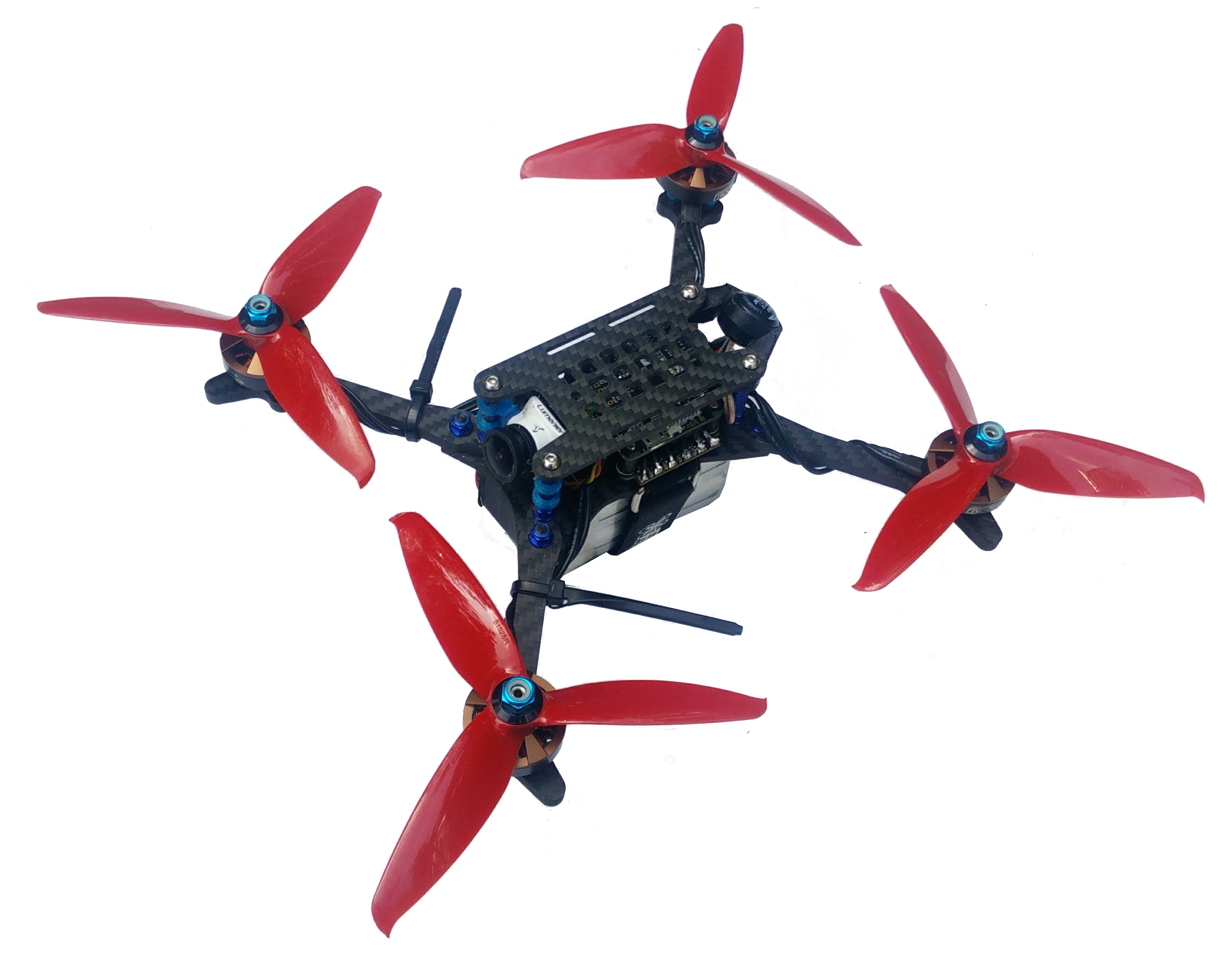
Figure 1$\cdot$1: FPV racing drone.

1.2 Scope and Contributions

Motivation for this work has been driven by drone racing. The sport of drone racing demands the highest level of flight performance to maintain a competitive edge. In drone racing, a UAV is remotely piloted by first-person-view (FPV). FPV provides an immersed flying experience allowing the UAV to be piloted from the perspective as if you were onboard the aircraft. This is accomplished by transmitting the video feed of an onboard camera to goggles with an embedded monitor worn by the pilot. The pilot manually controls the angular velocity (attitude) of the aircraft and mixes in throttle to achieve translational movements. A typical FPV equipped racing drone is pictured in Fig. 1$\cdot$1. A racing drone is an interesting CPS for studying control as they are capable of high speeds and aggressive maneuvers. Furthermore the controller is exposed to a number of nonlinear dynamics.

Using a racing drone as our experimental platform we study the aforementioned challenges for synthesizing neuro-controllers. In response to the study, the main contribution of this dissertation is a full solution stack depicted in Fig. 1$\cdot$2 for synthesizing neuro-flight controllers. This stack includes a simulation training environment, digital twin modelling methodology, and flight control firmware.

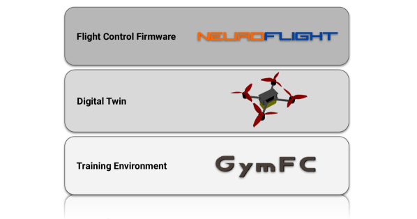
Figure 1$\cdot$2: Neuro-flight controller solution stack.

Throughout this dissertation we synthesize neuro-controllers for the quadcopter aircraft, however the training methods described in this work are generic to most space and aircraft. Specifically our contributions are in training low level attitude controllers. Previous work [Kim et al., 2004, Abbeel et al., 2007, Hwangbo et al., 2017, dos Santos et al., 2012, Palossi et al., 2019] has focused on high level navigation and guidance tasks, while it has remained unknown how well these type of controllers perform for low level control.

This dissertation is scoped to synthesizing neuro-controllers offline in simulation. This is a precursor for practical deployment as the controller must have initial knowledge of how to achieve stable flight. We provide an initial study of these type of controllers and publish open source software and frameworks for researchers to progress their performance. For neuro-controllers to be adopted in the future we believe a hybrid solutions that incorporates online learning methods to compensate for unmodelled dynamics in the simulation environment will be required. However as the saying goes, one must learn to walk before one can run.

Given the capacity and potential of NNs, we believe they are the future for developing high performance, reliable flight control systems. Our contributions and impact are predominately in the development and release of open source software allowing others to build off of our work to advance the progression in intelligent flight controller design. We will now briefly summarize the contributions of each item in the solution stack.

1.2.1 Tuning Framework and Training Environment

Most control algorithms are associated with a set of adjustable parameters that must be tuned for their specific application. Tuning a flight controller in the real world is a time consuming task and few systematic approaches are openly available. Simulated environments, on the other hand, are an attractive option for developing automated systematic methods for tuning. They are cost effective, run faster than real time, and easily allow software to automate tasks.

The benefits of a simulated environment for tuning flight controllers is not unique to RL-based controllers, but also applies to traditional controllers as well. In the context of neuro-controllers, training is just the process of tuning the NNs weights. In summary this dissertation makes the following contributions in controller tuning and RL training environments.

GymFC: The first item in our solution stack is an open source tuning framework for synthesizing neuro-flight controllers in simulation called GymFC. GymFC was originally developed as an RL training environment for synthesizing attitude flight controllers. The initial environment architecture is introduced in Chapter 3 and has been published in [Koch et al., 2019b]. Since the projects release GymFC has matured into a generic universal tuning framework based on feedback received from the community. Revisions to GymFCv1, discussed in Chapter 5, increase user flexibility providing a framework to provide custom reward systems and aircraft models. Additionally GymFC is no longer tied to an RL environment but now opens up the possibilities for other optimization algorithms to tune traditional controllers. In Chapter 5 we demonstrate the modular design of the framework by implementing a dynamometer for validating motor models in simulation, and a PID controller tuning system. Our goal with GymFC is to provide the research community a standardized way for tuning flight controllers in simulation. The source code is available at [Koch, 2018a].

Flight control reward system: In the context of RL-based flight controllers the training environment must provide the agent with a reward they are doing the right thing. This dissertation shows the progression of our reward system development to synthesize accurate controllers and address challenges transferring controllers to the real world. In Chapter 3 we introduce rewards to minimize error which has also been published in [Koch et al., 2019b]. From experimentation we find in Chapter 4 that additional rewards are necessary in order to transfer the trained policy into hardware which also appear in [Koch et al., 2019a]. As the accuracy of our aircraft model continued to increase we fine tuned the reward system in Chapter 5 to decrease error.

RL evaluation: The field of RL is progressing rapidly and a number of algorithms have been proposed for continuous control tasks. The RL algorithm can be thought of as the NN tuner. It determines how the NN weights are updated depending on the agents current, and past interactions with the environment and rewards received. This dissertation does not introduce new RL algorithms but instead uses off-the-shelf implementations for the purpose of synthesizing flight controllers. Specifically this dissertation makes its contribution in the performance evaluation of several state-of-the-art RL algorithms, including Deep Deterministic Policy Gradient (DDPG) [Lillicrap et al., 2015], Trust Region Policy Optimization (TRPO) [Schulman et al., 2015], and Proximal Policy Optimization (PPO) [Schulman et al., 2017]. These results were first published in [Koch et al., 2019b].

1.2.2 Digital Twin Development

Every aircraft is unique in its own way. Off the assembly line, accumulation of tolerances of each individual part from the manufacturing process results in a slightly different aircraft. In some cases performance between the same parts, such as sensors, can vary greatly [Miglino et al., 1995]. Once an aircraft is put into service, they continue to diverge from their initial state as they age.

To maximize performance, a controller would ideally be synthesized uniquely for each individual aircraft, at least in the scope of offline training strategies. To synthesize this controller in simulation, what we need is a digital replica, or digital twin of the aircraft. A digital twin is a relatively new paradigm, generic to digitizing any CPS which resides in an ultra high fidelity simulator. Once the CPS is put into service, it is kept in synchronization with its digital twin through the collection of state information from its senors. Typical use cases for the digital twin are for analytics, design and forecasting failures.

This work is the first to fuse together digital twinning concepts for neuro-flight controller training. In contrast, previous work has primarily used a mathematical model of the UAV [Hwangbo et al., 2017, Waslander et al., 2005, Kim et al., 2004, Abbeel et al., 2007] rather than a physics simulator. In summary we make the following contributions in digital twinning.

Multicopter Digital Twin Development Processes: Most flight control research performed in simulation use prebuilt aircraft models from Gazebo [Koenig and Howard, 2004] or PX4 [Meier et al., 2015] as they are readily available. In Chapter 3 for our initial feasibility analysis, we also took this approach using the Iris quadcopter [iri, 2018] model provided by Gazebo. We improved the motor models to more accurately reflect the motors used by our real quadcopter in Chapter 4. Lastly in Chapter 5 we provide our methodology for creating a digital twin from the ground up and apply these processes to create a digital twin of our custom built racing quadcopter.

Our novel dynamometer for identifying parameters of our propulsion system repurposes the avionics to capture the electronic dynamics that would be experienced during flight which cannot otherwise be captured from commercial dynamometers. This results in a higher fidelity motor model which encodes dynamics such as power delivery from the electronic speed controller (ESC) and control signal latency.

Our contributions are in the initial construction of the digital twin, we do not maintain synchronization with the twin after the aircraft is deployed in this work. Although our development is specific our quadcopter, these processes are applicable to any multicopter.

Propulsion System Models: The performance capabilities of a multicopters propulsion system (motor and propeller pair) have a large influence in the overall performance of the aircraft. This work builds upon the software in the loop (SITL) motor models developed by the PX4 firmware project [px4, 2019]. These models have been ported to GymFC and we have introduced additional dynamics to increase realism such as motor response and throttle curve mapping. These models have been made open source available from [Koch, 2019a].

Simulation Stability Analysis: Multicopters (particular those found in racing) are capable of achieving high angular velocities, which induce large centripetal forces. Under certain circumstances this can result in the digital twin becoming unstable in simulation. In this work we discuss the conditions in which instabilities can occur. We also propose an algorithm for measuring simulation stability and have included an implementation with GymFC [Koch, 2018a]. Using this software we perform an analysis of our digital twin.

1.2.3 Flight Control Firmware

Common approaches for deploying a neuro-controller to a UAV is to use a companion computer and run the NN in user space. However this is usually only suitable for slower than real-time applications that do not have strict deadlines and the UAV can permit the size, and weight of the additional hardware. Companion computers are typically used for high level control tasks such as navigation and guidance in flight control systems which need the additional computational resources but have a slower control loop in comparison to the low level stability control.

To meet control loop timing requirements, UAVs currently use microcontrollers to execute the real-time task of low level flight control. However there previously did not exist solutions for deploying neuro-controllers to microcontrollers let alone a flight control firmware that supported neuro-controllers.

To evaluate our neuro-controllers trained in simulation in the real world it was first necessary for us to develop methods for compiling a NN to run on a microcontroller. With these methods established we developed the flight control firmware Neuroflight to support neuro-attitude flight controllers. The results from this work first appeared in [Koch et al., 2019a]. In summary, this dissertation makes the following contributions in the area of flight control firmware.

Neuroflight: Prior to this work, every open source flight control firmware available used PID control [Ebeid et al., 2018]. In this work we have created the world’s first open source NN supported flight control firmware for UAVs, Neuroflight. The firmware provides the community with a platform to experiment with their own trained policies and further progress advancements in field of flight control. The source code is available from [Koch, 2018b].

Toolchain: The target hardware for most UAV flight control firmware is significantly resource constrained. The off-the-shelf microcontrollers supported by the family of high performance drone racing firmwares only consists of 1MB of flash memory, 320KB of SRAM and an ARM Cortex-M7 processor with a clock speed of 216MHz [STM, 2018]. This dissertation proposes a toolchain to allow NNs to be compiled to run on off-the-shelf microcontrollers with hard floating point arithmetic. The impact of this toolchain reaches beyond flight control for UAVs and opens up the possibilities of using neuro-control for other CPS’s in resource constrained environments.

Flight Performance Evaluation: In the context of low level attitude control, this work provides the first evaluation of a neuro-controller trained in simulation and transferred to hardware to fly in the real world. Our timing analysis reveals the NN-based attitude control task is able to execute at over 2kHz on an Arm Cortex-M microcontroller. We demonstrate our training environment, and reward functions are capable of synthesizing controllers with remarkable performance in the real world. Our real world flight evaluations validate these controllers are capable of stable flight and the execution of aerobatic maneuvers.

1.3 Structure

In summary, the remainder of this dissertation is organized as follows. In Chapter 2 we discuss important background information and related work pertinent to synthesizing neuro-based flight controllers. In Chapter 3 we present our flight control training environment GymFC and provide a feasibility analysis on whether neuro-flight controllers can accurately provide attitude control in simulation. To identify if the synthesized controllers can achieve stable flight in the real world we present our firmware, Neuroflight and its accompanying toolchain in Chapter 4. We propose our digital twin development methodology in Chapter 5 and introduce our revisions to GymFC to support training of arbitrary aircraft models. Finally in Chapter 6 we conclude with our final remarks and future work.

Chapter 2 Background and Related Work

In this chapter we discuss background concepts and related work. We begin in Section 2.1 with the history and evolution of flight control for fixed wing aircraft leading up to the rise of the quadcopter. In Section 2.2 we provide an overview of quadcopter flight dynamics and review flight control systems found in commercial UAVs in Section 2.3. In Section 2.4 we discuss flight control research being conducted in academia and the trend towards intelligent control systems. In Section 2.4.1 we emphasize the academic research related to deep reinforcement learning in the context of flight control. To successfully transfer models from simulation to hardware a number of strategies have been proposed which we review in Section 2.5. Lastly we provide an overview of digital twinning in Section 2.6 particularity in the context of flight control.

2.1 History of Flight Control

Aviation has a rich history in flight control dating back to the 1960s. During this time supersonic aircraft were being developed which demanded more sophisticated dynamic flight control than what a linear controller could provide. Gain scheduling [Leith and Leithead, 2000] was developed allowing multiple linear controllers of different configurations to be used in designated operating regions. This however was inflexible and insufficient for handling the nonlinear dynamics at high speeds but paved way for adaptive control.

During the 1950s there was a period know as the brave era in which various adaptive control techniques were tested with little time between conception and implementation. The lack of theoretical analysis and guarantees resulted in fatalities most notably in the X-15 crash [Hovakimyan et al., 2011]. Eventually this led to the development of Model Reference Adaptive Control (MRAC) [Whitaker et al., 1958] which introduced a reference model specifying the desired performance of the controller during adaptation. A reference model usually consists of the transient response characteristics such as rise time, setting time and steady state error. However early developments of MRAC did not have stability guarantees during adaptation. It was not until later that MRAC used the Lyapunov function for stability [Åström and Wittenmark, 2013]. To improve upon tuning challenges found in MRAC, $L_{1}$ was proposed which includes a lowpass filter to decouple the rate of adaptation and robustness. An $L_{1}$ control system was tested in the U.S. Air Force’s VISTA F-16 aircraft [Farha, 2016]. However there has been considerable debate in the control community due to two rebuttal papers questioning the true benefits of $L_{1}$ adaptive control [Black et al., 2014].

There has been a trend towards using artificial intelligence for adaptive control in fixed wing crewed aircraft to compensate for the nonlinear aircraft dynamics, and uncertainties. Specifically the use of artificial NNs which provide capabilities that are beyond that of traditional control such as their ability to learn and approximate any function. For an introduction to NNs with applications to control we refer to [Hagan and Demuth, 1999].

Work provided by [Kim et al., 1993] sought to create a single controller valid throughout the entire flight envelope to remove the need for gain scheduling. The use of nonlinear controllers such as feedback linearization are an attractive option as they are able to transform the nonlinear system into an equivalent linear representation. Once in a linear representation a linear controller, such as PID or linear quadratic Gaussian (LQG) can be used. However feedback linearization requires a model of the aircraft which can contain errors. To develop an aircraft model, the authors utilized a NN which is first trained offline using mathematical models, and then fine tuned, online using a second NN to compensate for any model errors. Another interesting contribution to this work was the use of the circle theorem [Zames, 1966] as a way to bound the stability of this controller even in the presence of the NNs.

The Intelligent Flight Control System (IFCS) project lead by NASA was created to investigate the capabilities of NNs for adaptive control, with a focus in providing stability during failure [Williams-Hayes, 2005]. Failure in this work is scoped to malfunctioning of the control surfaces. The project’s test aircraft is a highly modified F-15; however this work only reports simulation results. Simulation results demonstrate the NN is able to restore the aircraft to a stable state after the occurrence of failure, in less time and smoother than without the presence of the NN. Starting in 2006 real flight tests began [Smith et al., 2010]. During these test flights, two failures were emulated, locking of the left stabilator and change to the baseline angle of attack of the canard (a small forward wing). Overall the test pilots reported improved handling with the NN enabled during failure. These results show a promising future for these type of controllers.

As a result of the significant cost reduction for sensors and small-scale embedded computing platforms over the course of the last couple decades, UAVs, particularity quadcopters, have surged in popularity. Due to their unique complex dynamics quadcopters have their own set of challenges related to flight control. However we are seeing similar patterns in the progress of flight control for UAVs as we have seen for fixed wing crewed aircraft. Although this dissertation’s focus is in the development of flight controllers for quadcopters, nonetheless the majority of what is discussed is applicable to most multicopter configurations and fixed wing aircraft as well.

2.2 Quadcopter Flight Dynamics

Before we can discuss the specifics of flight control pertaining to the quadcopter aircraft it is necessary to understand some basics of their dynamics.

A quadcopter is an aircraft with four (quad) motors using a propeller propulsion system. It has six degrees of freedom (DOF), three rotational and three translational as depicted in Fig. 2$\cdot$1. Throughout this dissertation we will use the motor ID and order referenced in this figure, starting at index one, to be consistent with the ordering used to configure our flight control firmware, while the subscript used in the mathematical notation begins with zero. We indicate with $\omega_{i},i\in{0,\dots,M-1}$ the rotation speed of each rotor where $M=4$ is the total number of motors for a quadcopter. These have a direct impact on the resulting Euler angles $\phi,\theta,\psi$, i.e., roll, pitch, yaw respectively and translation in each $x$, $y$, and $z$ direction.

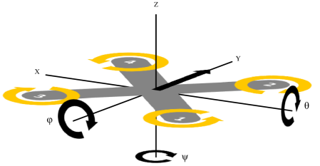
Figure 2$\cdot$1: Axis of rotation

The aerodynamic effect that each $\omega_{i}$ produces depends upon the configuration of the motors. The motor configuration (i.e., location of each motor) can have a significant affect in flight performance depending on the distance the motors are from each axis of rotation. Intuitively the greater the distance the motor is from the axis of rotation the more torque will be required to travel along this arc compared to when a motor is mounted closer to the axis. In the context of classical mechanics, torque is defined as $\tau=l\times F$ where $l$ is the length of the lever and $F$ is the applied force. Translated to a quadcopter, each motor and propeller pair generates a force $F$ at some distance $l$ from the axis of rotation.

The most popular configuration is an X configuration, depicted in Fig. 2$\cdot$1 which has the motors mounted in an X formation relative to what is considered the front of the aircraft. This configuration provides more stability compared to a + configuration which in contrast has its motor configuration rotated an additional $45^{\circ}$ along the z-axis. This is due to the differences in torque generated along each axis of rotation in respect to the distance of the motor from the axis. Additionally the X configuration is a more practical arrangement for mounting cameras used for navigation.

For a + configuration the distance, in relation to pitch, is equivalent to the distance of the arm $l$. An X configuration with the same arm length $l$ has a distance from the axis $l\times cos(\pi/4)$ resulting in less torque required. A decrease in the arm length provides increased responsiveness. Furthermore the motor rotation in a + configuration is in the same direction along an axis of rotation leading to less stability than an X configuration. Based on these dynamics, frames are optimized depending on their application. For example racing frames are often stretched such that the distance between motors 3 and 4, and motors 1 and 2, are at a greater distance than between motors 1 and 3, and motors 2 and 4. This results in less torque along the roll axis providing a more responsive aircraft for performing turns.

The aerodynamic affect $U$ that each rotor speed $\omega_{i}$ has on thrust and Euler angles, is given by:

$$U_{T} =B(\omega_{0}^{2}+\omega_{1}^{2}+\omega_{2}^{2}+\omega_{3}^{2})$$ (2.1)

$$U_{\phi} =B(\omega_{0}^{2}+\omega_{1}^{2}-\omega_{2}^{2}-\omega_{3}^{2})$$ (2.2)

$$U_{\theta} =B(\omega_{0}^{2}-\omega_{1}^{2}+\omega_{2}^{2}-\omega_{3}^{2})$$ (2.3)

$$U_{\psi} =B(\omega_{0}^{2}-\omega_{1}^{2}-\omega_{2}^{2}+\omega_{3}^{2})$$ (2.4)

where $U_{T},U_{\phi},U_{\theta},U_{\psi}$ is the thrust, roll, pitch, and yaw effect respectively, while $B$ is a thrust factor that captures propeller geometry and the motor configuration. The torque $\tau_{B}$ applied to the aircraft is the torque applied to each axis $\phi,\theta,\psi$ for roll, pitch, yaw respectively. The model developed by [Luukkonen, 2011, Bouabdallah et al., 2004] modified for X configuration as,

$$\tau_{B}=\begin{bmatrix}\tau_{\phi}\\ \tau_{\theta}\\ \tau_{\psi}\\ \end{bmatrix}=\begin{bmatrix}lcos(\pi/4)B(\omega_{0}^{2}+\omega_{1}^{2}-\omega_{2}^{2}-\omega_{3}^{2})\\ lcos(\pi/4)B(\omega_{0}^{2}-\omega_{1}^{2}+\omega_{2}^{2}-\omega_{3}^{2})\\ \sum_{i=0}^{M-1}\tau_{M_{i}}\end{bmatrix}$$ (2.5)

where $\tau_{M_{i}}$ is the torque of each motor.

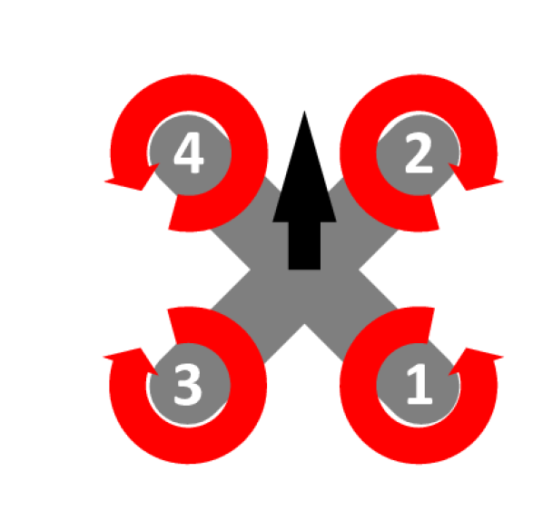
(a) Accel

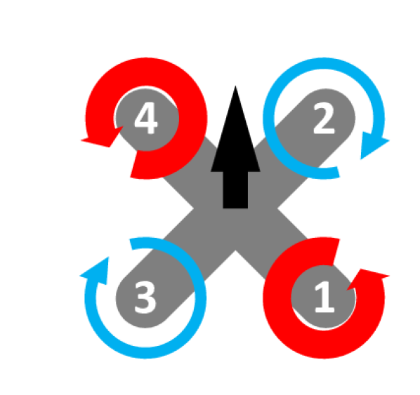
(b) Yaw CW

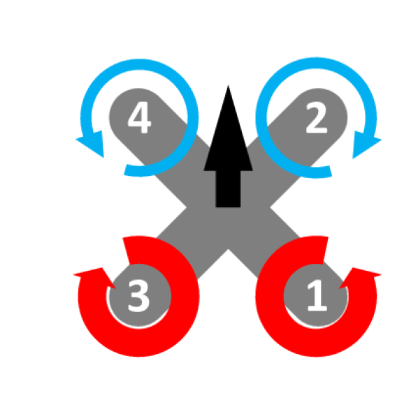
(c) Pitch forward

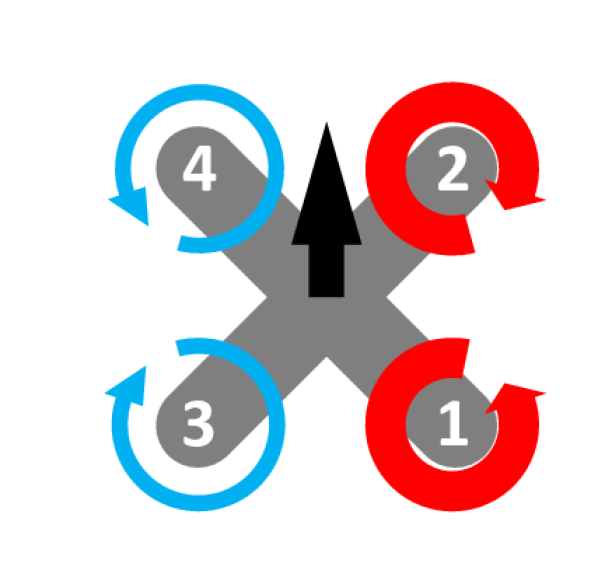
(d) Roll left

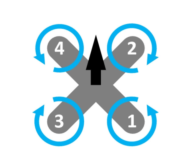
(e) Decel

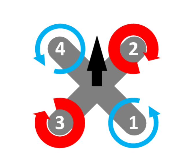
(f) Yaw CCW

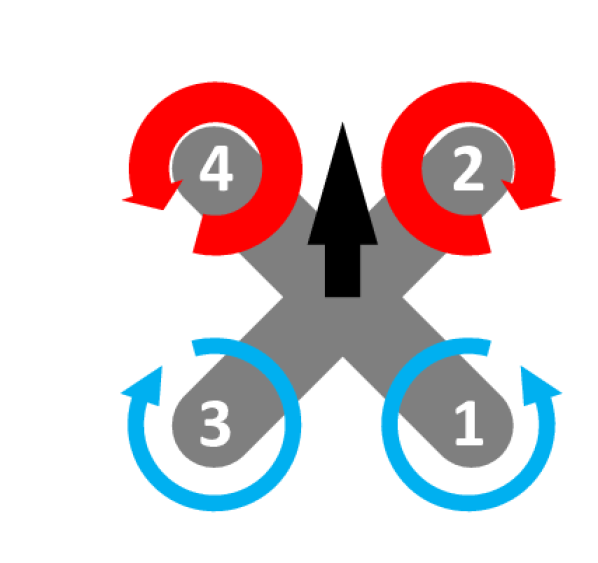
(g) Pitch backward

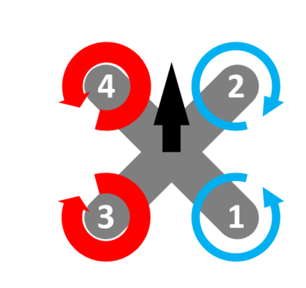
(h) Roll right

Figure 2$\cdot$2: Commands of a quadcopter. Red wide arrows represent faster angular velocity, while blue narrow arrows represent slower angular velocity. Faster and slower velocities are relative to when its net force is zero.

To perform rotational movement the velocity of each rotor is manipulated according to the relationship expressed in Eq. 2.2 Eq. 2.3, Eq. 2.4 and as illustrated in Fig. 2$\cdot$2. For example, to roll right (Fig. 2$\cdot$2(h)) more thrust is delivered to motor 3 and 4 (i.e., $\omega_{2}>\omega_{0}$ and $\omega_{3}>\omega_{1}$). However yaw is not achieved directly through difference in thrust generated by the rotor as roll and pitch are, but instead through a difference in torque generated by the velocity of the rotors. For example, as shown in Fig. 2$\cdot$2(b), higher rotational speed for rotors 1 and 4 allow the aircraft to yaw clockwise. A net positive torque of the rotors in the counter-clockwise direction causes the aircraft to rotate clockwise in the opposite direction due to Newton’s second law of motion.

Attitude, in respect to the orientation of the aircraft, can be expressed as the angular velocities of each axis $\Omega=[\Omega_{\phi},\Omega_{\theta},\Omega_{\psi}]$. The objective of attitude control is to compute the required motor control signals $u=[u_{0},\dots,u_{M-1}]$ to achieve some desired attitude $\Omega^{*}$. In autopilot systems attitude control is typically executed as an inner control loop and is time-sensitive. Once the desired attitude is achieved, translational movements (in the X, Y, Z direction) are accomplished by applying thrust proportional to each motor. For further details about the mathematical models of quadcopter dynamics please refer to [Bouabdallah et al., 2004].

2.3 Flight Control for Commercial UAVs

Of the commercially available flight control systems and open source flight control firmwares currently available every single one uses a static linear controller called proportional, integral, and derivative (PID) control [Ebeid et al., 2018].

A PID controller is a linear feedback controller expressed mathematically as,

$$y(t)=K_{P}e(t)+K_{I}\int_{0}^{t}e(\tau)d\tau+K_{D}\frac{de(t)}{dt}$$ (2.6)

where $K_{P},K_{I},K_{D}$ are configurable constant gains and $y(t)$ is the output. The effect of each term can be thought of as the P term considers the current error, the I term considers the history of errors and the D term estimates the future error. In the context of attitude control there is a PID controller to control each roll, pitch and yaw axis. The attitude controller controls the orientation of the aircraft, typically by its angular velocity. A PID attitude controller results in a total of 9 gains that must be collectively tuned for each aircraft.

Every time a PID attitude controller is evaluated, the PID for each axis is computed. The output of each of the PIDs must be combined together to form the control signal for each motor. This process is called mixing. Mixing uses a table consisting of constants to compensate for the motor configuration described in Section 2.2. The control signal for each motor $u_{i}$ is loosely defined as,

$$u_{i}=\mathbf{T}+m_{(i,\phi)}y_{\phi}+m_{(i,\theta)}y_{\theta}+m_{(i,\psi)}y_{\psi}$$ (2.7)

where $m_{(i,\phi)},m_{(i,\theta)},m_{(i,\psi)}$ are the mixer values for motor $i$ and $\mathbf{T}$ is the throttle.

To adapt to nonlinear dynamics experienced during flight, the firmware of some flight controllers (e.g., Betaflight [bet, 2018]) use gain scheduling. This gain scheduler adjusts the PID gains for certain operating regions such as the throttle value and battery voltage levels.

2.4 Flight Control Research in Academia

As flight control methods continue to develop for fixed wing crewed aircraft, accelerated growth in multicopters have forged new areas of research for this new bread of aircraft. This has been beneficial for flight control development in general as the low cost of a quadcopter has made it practical for anyone to engage in this research.

Quadcopters are naturally unstable and underactuated, meaning each of the six degrees of freedom cannot be controlled directly. These complex dynamics present an interesting control problem. In order to maintain stability, a quadcopter requires a control algorithm to calculate the power to apply to each motor.

In academia there has been extensive research in flight control systems for quadcopters [Zulu and John, 2014, Li and Song, 2012]. Optimal control algorithms have been applied using linear quadratic Gaussian (LQG) [Minh and Ha, 2010], and $H_{\infty}$ which minimize a specific cost function until an optimally defined criteria is achieved. However these algorithms tend to lack robustness [Zulu and John, 2014, Li and Song, 2012]. Adaptive control using feedback linearization [Palunko and Fierro, 2011] have also been applied which allows for the system control parameters to adapt to change over time however these algorithms typically rely on mathematical models of the aircraft.

Similar to flight control for crewed aircraft, there has also been a shift towards intelligent control methods for UAVs to address limitations of traditional control methods. Intelligent control is a control system that uses various artificial intelligent algorithms [Santoso et al., 2017]. These algorithms are broadly categorized into three different classes for what they provide: knowledge, learning and global search. Knowledge algorithms consist of fuzzy and expert systems, learning algorithms encompass NNs, and global search contains search and optimization algorithms such as genetic algorithms and swarm intelligence. Each of these algorithms have their own advantages and disadvantages when it comes to developing fight control systems. However knowledge and global search algorithms do not have the functionality and capabilities to provide direct control of the aircraft actuators. Knowledge-based algorithms are unable to adapt to new unseen events and lack robustness, qualities that are undesirable for control tasks with noisy sensors and complex nonlinear dynamics. While global search algorithms are far to time consuming for real-time control of an aircraft. NNs, on the other hand, have a number of characteristics that are attractive for control. They are universal approximators, resistant to noise [Miglino et al., 1995], and provide predictive control [Hunt et al., 1992].

Intelligent PID flight control [Fatan et al., 2013] methods have been proposed in which PID gains are dynamically updated online providing adaptive control as the environment changes. However these solutions still inherit disadvantages associated with PID control, such as integral windup, need for mixing, and most significantly, they are feedback controllers and therefore inherently reactive. On the other hand feedforward control (or predictive control) is proactive, and allows the controller to output control signals before an error occurs. For feedforward control, a model of the system must exist. Learning-based intelligent control has been proposed to develop models of the aircraft for predictive control using artificial NNs.

Notable work by [Dierks and Jagannathan, 2010] proposes an intelligent flight control system constructed with NNs to learn the quadcopter dynamics, online, to navigate along a specified path. This method allows the aircraft to adapt in real-time to external disturbances and unmodelled dynamics. Matlab simulations demonstrate that their approach outperforms a PID controller in the presence of unknown dynamics, specifically in regards to control effort required to track the desired trajectory. Nonetheless the proposed approach requires prior knowledge of the aircraft mass and moments of inertia to estimate velocities. While online learning is an essential component to construct a complete intelligent flight control system, nonetheless it is fundamental to develop accurate offline models to establish an initial stable controller. Offline learning can also teach the NN how to respond to rare occurring events ahead of time before encountering them in the real world [Santoso et al., 2017].

To build offline models, previous work has used supervised learning to train intelligent flight control systems using a variety of data sources such as test trajectories [Bobtsov et al., 2016], and PID step responses [Shepherd III and Tumer, 2010]. The limitation of this approach is that training data may not accurately reflect the underlying dynamics. In general, supervised learning on its own is not ideal for interactive problems such as control [Sutton and Barto, 1998].

There is, however, an alternative learning paradigm for building offline models that is ideal for continuous control tasks, does not make assumptions about the aircraft dynamics and is capable of creating optimal control policies. This learning paradigm is known as reinforcement learning (RL).

2.4.1 Flight Control via Reinforcement Learning

RL is a machine learning paradigm in which an agent interacts with its environment in order to learn a task over time. Deep RL refers to the use of a NN as the agent that contains two or more hidden layers. In this work we consider a deep RL architecture as depicted in Fig. 2$\cdot$3. We will now describe the agents interaction with the environment in the context of neuro-flight controller training.

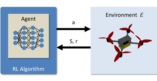
Figure 2$\cdot$3: Deep RL architecture.

At each discrete time-step $t$, the agent (i.e., NN) receives an observation $S_{t}$ from the environment $\mathcal{E}$. The environment consists of the aircraft and also the simulation world while observations are obtained through various sensors onboard the aircraft. Because the agent is only receiving sensor data, it is unaware of the entire physical environment and aircraft dynamics and therefore $\mathcal{E}$ is only partially observed by the agent. These observations are in the continuous observation spaces $S_{t}\in\mathbb{R}$. The observations are used as input to evaluate the agent to produce the action $a_{t}$. The action values are also in the continuous range $a_{t}\in\mathbb{R}^{M}$ and corresponds to the $M$ control signals to send to the ESC. This action is applied to the environment and in return the agent receives a single numerical reward $r_{t+1}$ indicating the performance of this action along with the updated state of the environment $S_{t+1}$.

In reality, during training, an RL algorithm acts as a shim between the agent and the environment. The RL algorithm uses the action, state, and reward history in order to adjust the weights of the NN.

The interaction between the agent and $\mathcal{E}$ is formally defined as a Markov decision processes (MDP) where the state transitions are defined as the probability of transitioning to state $s^{\prime}$ given the current state and action are $s$ and $a$ respectively, $Pr\{s_{t+1}=s^{\prime}|s_{t}=s,a_{t}=a\}$. The behavior of the agent is defined by its policy $\pi$ which is essentially a mapping of what action should be taken for a particular state. The objective of the agent is to maximize the returned reward overtime to develop an optimal policy. We invite the reader to refer to [Sutton and Barto, 1998] for further details on RL.

RL has similar goals to adaptive control in which a policy improves overtime interacting with its environment. RL has been applied to autonomous helicopters to learn how to track trajectories, specifically how to hover in place and perform various maneuvers  [Bagnell and Schneider, 2001, Kim et al., 2004, Abbeel et al., 2007]. Work by [Kim et al., 2004, Abbeel et al., 2007] validated their trained helicopter’s capabilities in helicopter competitions requiring the aircraft to perform advanced acrobatic maneuvers. Performance was compared to trained pilots, nevertheless it is unknown how their controllers compare to PID control for tracking trajectories.

The first use of RL in quadcopter control was presented by [Waslander et al., 2005] for altitude control. The authors developed a model-based RL algorithm to search for an optimal control policy. The controller was rewarded for accurate tracking and damping. Their design provided significant improvements in stabilization in comparison to linear control methods.

Up until recently control in continuous action spaces was considered difficult for RL. Significant progress has been made combining the power of NNs with RL. State-of-the-art algorithms such as Deep Deterministic Policy Gradient (DDPG) [Lillicrap et al., 2015], Trust Region Policy Optimization (TRPO) [Schulman et al., 2015] and Proximal Policy Optimization (PPO) [Schulman et al., 2017] have shown to be effective methods of training deep NNs [Duan et al., 2016, Koch et al., 2019b]. DDPG provides improvement to Deep Q-Network (DQN) [Mnih et al., 2013] for the continuous action domain. It employs an actor-critic architecture using two NNs for each actor and critic. It is also a model-free algorithm meaning it can learn the policy without having to first generate a model. TRPO is similar to natural gradient policy methods however this method guarantees monotonic improvements. PPO [Schulman et al., 2017] is known to out perform other state-of-the-art methods in challenging environments. PPO is also a policy gradient method and has similarities to TRPO. Its novel objective function allows for a Trust Region update to the policy at each training iteration. Many RL algorithms can be very sensitive to hyperparameter tuning in order to obtain good results. Part of the reason PPO is so widely adopted is due to it being easier to tune than other RL algorithms.

More recently [Hwangbo et al., 2017] has used deep RL for quadcopter control, particularly for navigation control. They developed a novel deterministic on-policy learning algorithm that outperformed TRPO [Schulman et al., 2015] and DDPG [Lillicrap et al., 2015] in regards to training time. Furthermore the authors validated their results in the real world, transferring their policy trained in simulation to a physical quadcopter. Path tracking turned out to be adequate. However the authors discovered major differences transferring from simulation to the real world.

The vast majority of prior work has focused on performance of navigation and guidance. There is limited and insufficient data justifying the accuracy and precision of NN-based intelligent attitude flight control and none previously for controllers trained via RL.

2.5 Transfer learning

The desire to train and evaluate intelligent control systems in simulation dates back to the 1990s as discussed in [Husbands and Harvey, 1992]. It is simply not practical to accomplish most training tasks in the real world as it would take far to long and be costly. However the fidelity and accuracy of the simulator drastically determines the controllers performance in the real world, in fact in some cases robots trained in simulated environments completely fail when transferred to a robot in the real world [Brooks, 1992]. To address these issues several studies have proposed methods to reduce the reality gap.

In [Miglino et al., 1995] the authors developed a simulator to train a neuro-controller for a two wheeled Khepera robot using evolutionary algorithms. The inputs of the NN was connected directly to eight infrared sensors, and the output was connected directly to two motors. During their research they found the accuracy of the infrared sensors varied drastically from one another. To adjust for these discrepancies in simulation the robot sensors were randomly sampled in the real world. To compensate for changes in light conditions noise was introduced in the simulated environment. Models of the robots motors were constructed in a similar way introducing noise to account for uncertainties in the environment (e.g., imperfections on the floor). Individuals were evaluated based on how fast they were able to travel in a straight line while still avoiding obstacles. Results show the robot had decreased in performance when transferred to a real robot, however continued training in the real world for a small number generations can revert and actually improve performance. The major contribution of this paper demonstrates the reality gap can be greatly reduced by introducing noise into the training data. Noise accounts for uncertainties found in the real world, as NNs are noise resistant the NN is able to learn the underlying dynamics despite the additional noise.

Around the same time, work by [Jakobi et al., 1995] explored three claims made by [Husbands and Harvey, 1992] to reduce the reality gap. First, a large amount of empirical data should be collected from the robots sensors, actuators and operating environment to be used to build accurate simulation environments. The authors discuss what is now referred to as hardware in the loop (HITL) as a method to further increase the accuracy by using the actual hardware of the robot. Second, noise should be injected at all inputs to blur the two running environments together. Third, adaptive noise tolerant elements should be used to absorb the discrepancies in the simulated environment from the real world.

The authors also performed their evaluations with the Khepera robot. First, mathematical models for each sensor and actuator in the system was defined based on elementary physics and control theory. Several experiments were conducted to collect empirical data on these devices and then mapping techniques were created to map the calculated value to the sampled value. To identify the ideal amount of noise to introduced into the simulation the NN was trained on three noise levels: zero, observed, and double observed. Observed noise is created from a Gaussian distribution with the standard deviation equal to that of the collected empirical data. Results verify previous work claims that the addition of noise in the simulator provides improved performance in the real world. Furthermore it was found that the normal observed noise level provided the best performance of the three. However there is a fine line in the amount of noise that is best, in some cases injecting double the observed noise performed worse than no noise at all.

If neuro-controllers synthesized in simulation via RL are to be adopted for use in real CPS, it is critical to reduce the reality gap. There have been several studies addressing the reality gap in the context of RL.

In [Tobin et al., 2017], the authors explore a method called domain randomization for reducing the reality gap. Domain randomization randomizes parts of the simulation environment with the idea being if the simulation has enough variety, the real world will just appear as another variation to the agent. In relation to the use of noise, domain randomization is a generalized method for adding variation to the environment which consists of the use of noise. The authors particular application is in computer vision in which a NN is trained to detect the location of an object. They randomize the location, number and shape of the objects. Additionally textures of object and environment were randomized. Similar to [Miglino et al., 1995] noise and also lighting conditions were also randomized. Their evaluation shows that domain randomization can provide high enough accuracy to locate and grasp an object from clutter.

In more recent work by [Andrychowicz et al., 2018] the authors applied deep RL to learn dexterous in-hand manipulation, a task that is beyond the capabilities of traditional control methods. The intention of this work is to show transferability of the learned policy to a real robot. To overcome the reality gap, the authors randomized most aspects of the simulation environment. In addition to applying noise to the observations, and randomizing visual properties they also randomized physical parameters such as friction and introduce delays and noise to the actions. Although domain randomization did narrow the reality gap, the real robot performed worse than in simulation. Transferability was most successful when the entire training environment state was randomized but they did point out that the affects of observation randomization had the least impact which they attribute to the accuracy of their motion capture system. Another interesting observation was the fact that training on a randomized environment converged significantly slower, than when trained without randomization.

In the context of flight control, authors in [Molchanov et al., 2019] investigate domain randomization for a RL-based stabilization flight controller. Particularity their focus is in developing a policy that can be transferred to multiple different quadcopter configurations. In this work they randomize the mass, the motor distance, motor response, torque and thrust characteristics. Training was conducted in their own simulation using mathematical models for the quadcopter dynamics. A Tensorflow based learning framework was used for training and the trained policy was transfer to hardware by extracting the trained NN parameters from the Tensorflow model to a custom NN C library. Policy evaluation was performed on three different quadcopters. Their results show the policy trained for a specific aircraft, without randomization performed best. Similar observations to [Andrychowicz et al., 2018] were reported in which domain randomization provided moderate improvements. Full randomization generalized better but other policies provided better performance for each particular aircraft.

To further reduce the reality gap and easy the transfer to hardware it is essential to increase the accuracy of the aircraft model (i.e., digital twin) used in simulation during training.

2.6 Digital Twinning

The concept of digital twinning was first introduced in Michael Grieves’s course on Product Lifecycle Management (PLM) in 2003 [Grieves, 2014]. He defines the digital twin concept to consist of three main parts, the physical asset in the real space, the virtual asset in virtual space, and a data connection link between these two spaces. With the rise of CPS, there is a plethora of sensor data available fueling new applications for digital twins.

In work provided by [Gabor et al., 2016] a generic software architecture for the integration of digital twins is proposed. There has been a paradigm shift from classical simulation architectures as the cognitive system (i.e., the system consisting of the logic to perform some desired functionality) now as the ability to communicate with both the physical world (i.e., the hardware) and a simulator (i.e., digital twin). From the CPS’s software perspective it should be indistinguishable whether it is interacting with hardware or its digital twin. Thus it is required the hardware and digital twin must implement identical interfaces. The authors introduce an observer design pattern to allow subcomponents in the software architecture to communicate.

Although the digital twinning concept was initially described in the context of manufacturing, in regards to aviation it has been adopted by NASA for vehicle health management [Glaessgen and Stargel, 2012] and GE Aviation for jet engine analytics and modelling.

Digital twinning has been proposed as a method to optimize practices regarding certification, fleet management and sustainment of future NASA and U.S. Air Force vehicles [Glaessgen and Stargel, 2012]. Current approaches are inefficient. Based on insufficient data of the aircraft, assumptions about system health are made based on statistics and heuristics from past observations and experiences. This can lead to unnecessary inspections, or worse, result in damage for an aircraft that has a unique, previously unseen experience. As next generation aircraft become more sophisticated, greater introspection of the individual aircraft will be required. A digital twin can address these issues by providing near real-time analytics and state of an individual aircraft. More specifically the authors describe the use of digital twins to provide a method to continuously predict the health of the aircraft. This has remarkable benefits such as the ability to predict future failures and address them early on before they become severe.

A digital twin is just one of the technologies used as part of larger vision of NASA’s to create self-aware vehicles [Tuegel et al., 2011]. The authors define a self-aware vehicle as “an aircraft, spacecraft or system is one that is aware of its internal state, has situational awareness of its environment, can assess its capabilities currently and project them into the future, understands its mission objectives, and can make decisions under uncertainty regarding its ability to achieve its mission objectives.”

Digital twinning provides the self-aware vehicle with the ability to monitor system health in real-time and forecast failures before they occur. This results in unparalleled degree of safety. Depending on the current aircraft state, a flight envelope can be uniquely establish to ensure predictable performance while operating in that range. Furthermore sensor data is relayed back to a ground stations to utilize the collective computational power of server farms to further assess the state of the aircraft.

In this dissertation we incorporate digital twinning concepts as a method to synthesize optimal flight controller policies that are unique to each individual aircraft.

Chapter 3 Reinforcement Learning for UAV Attitude Control

Over the last decade there has been an uptrend in the popularity of UAVs. In particular, quadcopters have received significant attention in the research community where a significant number of seminal results and applications have been proposed and experimented. This recent growth is primarily attributed to the drop in cost of onboard sensors, actuators and small-scale embedded computing platforms. Despite the significant progress, flight control is still considered an open research topic. On the one hand, flight control inherently implies the ability to perform highly time-sensitive sensory data acquisition, processing and computation of forces to apply to the aircraft actuators. On the other hand, it is desirable that UAV flight controllers are able to tolerate faults; adapt to changes in the payload and/or the environment; and to optimize flight trajectory, to name a few.

Autopilot systems for UAVs are typically composed of an “inner loop” responsible for aircraft stabilization and control, and an “outer loop” to provide mission level objectives (e.g., way-point navigation). Flight control systems for UAVs are predominately implemented using the Proportional, Integral Derivative (PID) control systems. PIDs have demonstrated exceptional performance in many circumstances, including in the context of drone racing, where precision and agility are key. In stable environments a PID controller exhibits close-to-ideal performance. When exposed to unknown dynamics (e.g., wind, variable payloads, voltage sag, etc), however, a PID controller can be far from optimal [Maleki et al., 2016]. For next generation flight control systems to be intelligent, a way needs to be devised to incorporate adaptability to mutable dynamics and environment.

The development of intelligent flight control systems is an active area of research [Santoso et al., 2017], specifically through the use of NNs which are an attractive option given they are universal approximators and resistant to noise [Miglino et al., 1995].

Online learning methods (e.g., [Dierks and Jagannathan, 2010]) have the advantage of learning the aircraft dynamics in real-time. The main limitation with online learning is that the flight control system is only knowledgeable of its past experiences. It follows that its performances are limited when exposed to a new event. Training models offline using supervised learning is problematic as data is expensive to obtain and derived from inaccurate representations of the underlying aircraft dynamics (e.g., flight data from a similar aircraft using PID control) which can lead to suboptimal control policies [Bobtsov et al., 2016, Shepherd III and Tumer, 2010, Williams-Hayes, 2005]. To construct high-performance intelligent flight control systems it is necessary to use a hybrid approach. First, accurate offline models are used to construct a baseline controller, while online learning provides fine tuning and real-time adaptation.

An alternative to supervised learning for creating offline models is RL. Using RL it is possible to develop optimal control policies for a UAV without making any assumptions about the aircraft dynamics. Recent work has shown RL to be effective for UAV autopilots, providing adequate path tracking [Hwangbo et al., 2017]. Nonetheless, previous work on intelligent flight control systems has primarily focused on guidance and navigation.

Open Challenges in RL for Attitude Control RL is currently being applied to a wide range of applications. each with its own set of challenges. Attitude control for UAVs is a particularly interesting RL problem for a number of reasons. We’ve highlighted three areas we find important below:

• Precision and Accuracy: Many RL tasks can be solved in a variety of ways. For example, to win a game there may be a number of sequential moves that will lead to the same outcome. In the case of optimal attitude control there is little tolerance and flexibility as to the sequence of control signals that will achieve the desired attitude (e.g. angular rate) of the aircraft. Even the slightest deviations can lead to instabilities. It remains unclear what level of control accuracy can be achieved when using intelligent control trained with RL for time-sensitive attitude control — i.e. the “inner loop”. Therefore determining the achievable level of accuracy is critical in establishing if RL is suitable for attitude flight control.

• Robustness and Adaptation: In the context of control, robustness refers to the controllers performance in the presence of uncertainty when control parameters are fixed while adaptiveness refers to the controllers performance to adapt to the uncertainties by adjusting the control parameters [Wang and Zhang, 2001]. It is assumed the NN trained with RL will face uncertainties when transfer to physical hardware due to the reality gap. However it remains unknown what range of uncertainty the controller can operate safely before adaptation is necessary. Characterizing the controllers robustness will provide valuable insight into the design of the intelligent flight control system architecture. For instance what will be the necessary adaptation rate and what sensor data can be collected from the real world to update the RL environment.

• Reward Engineering: In the context of attitude control, the reward must encapsulate the agent’s performance achieving the desired attitude goals. As goals become more complex and demanding (e.g. minimizing energy consumption, or stability in presence of damage ) identifying which performance metrics are most expressive will be necessary to push the performance of intelligent control systems trained with RL.

Our Contributions In this chapter we study in-depth C1, the accuracy and precision of attitude control provided by intelligent flight controllers trained using RL. While we specifically focus on the creation of controllers for the Iris quadcopter [iri, 2018], the methods developed hereby apply to a wide range of multi-rotor UAVs, and can also be extended to fixed-wing aircraft. We develop a novel training environment called GymFC with the use of a high fidelity physics simulator for the agent to learn attitude control. This being the initial release, it will be referred to as GymFCv1 for the remainder of the chapter. GymFCv1 is an OpenAI Environment [Brockman et al., 2016] providing a common interface for researchers to develop intelligent flight control systems. The simulated environment consists of an Iris quadcopter digital twin [Gabor et al., 2016]. The intention is to eventually be able to transfer the trained policy to physical hardware. Controllers are trained using state-of-the-art RL algorithms: Deep Deterministic Policy Gradient (DDPG), Trust Region Policy Optimization (TRPO), and Proximal Policy Optimization (PPO). We then compare the performance of our synthesized controllers with that of a PID controller. Our evaluation finds that controllers trained using PPO outperform PID control and are capable of exceptional performance. To summarize, this chapter makes the following contributions:

• GymFCv1, an open source [Koch et al., 2019b] environment for developing intelligent attitude flight controllers while providing the research community a tool to progress performance.

• A learning architecture for attitude control utilizing digital twinning concepts for minimal effort when transferring trained controllers into hardware.

• An evaluation for state-of-the-art RL algorithms, such as Deep Deterministic Policy Gradient (DDPG), Trust Region Policy Optimization (TRPO), and Proximal Policy Optimization (PPO), learning policies for aircraft attitude control. As a first work in this direction, our evaluation also establishes a baseline for future work.

• An analysis of intelligent flight control performance developed with RL compared to traditional PID control.

The remainder of this chapter is organized as follows. In Section 3.1 we review simulation environments and architectures currently used for training RL policies. In Section 3.3 we present our training environment and use this environment to evaluate RL performance for flight control in Section 3.4. Finally Section 3.5 concludes the chapter and provides a number of future research directions.

3.1 Background and Related Work

The release of OpenAI Gym [Brockman et al., 2016] made a huge splash in the RL community providing a common API for RL environments and a repository of various environments implementing this API. This common API has had a large impact on RL algorithm evaluations and has become the staple for benchmarking new algorithms. Since its release a number of popular RL algorithm libraries have added supported for OpenAI Gym including OpenAI Baselines [Dhariwal et al., 2017], Stable Baselines [Hill et al., 2018], Tensorforce [Schaarschmidt et al., 2017], Keras-RL [Plappert, 2016], and TF-Agents [Sergio Guadarrama, Anoop Korattikara, Oscar Ramirez, Pablo Castro, Ethan Holly, Sam Fishman, Ke Wang, Ekaterina Gonina, Neal Wu, Chris Harris, Vincent Vanhoucke, Eugene Brevdo, 2018].

Creating an instance of the environment is as easy as calling gym.make(env_id) in which env_id is a string representing the unique ID of the environment. The simplistic environment creation is beneficial for benchmarking purposes as it provides a consistent environment. Nonetheless, this is an issue for more complex environments that have the intention of using the trained policy in the real world. One could argue for a specific application there is no need for a common API. However one of the advantages of the Gym API as we previously mentioned is the vast adoption of the API by RL algorithm libraries. This allows one to stand up a training environment with only a few lines of code and easily allow users to switch from one RL algorithm to another.

Within the collection of environments, a number of continuous control environments exist such as controlling a lunar lander, race car, and a bipedal walker. Additionally there exist robotic tasks such as hand manipulation using the MuJoCo physics engine [Todorov et al., 2012]. Using OpenAI Gym’s API, researchers and developers have begun to create their own environments.

Gazebo [Koenig and Howard, 2004] is a mature open source high fidelity simulator and has been used as a simulator backend for training environments. It is also a popular simulator choice for SITL and HITL testing of flight control firmware projects, for example Betaflight [bet, 2018], PX4 [Meier et al., 2015] and Ardupilot [ard, 2018]. Gazebo supports the open source physics engines ODE [Smith, Russel, 2006], Bullet [Coumans, 2015], Simbody [Sherman et al., 2011] and DART [Lee et al., 2018] giving the user the flexibility to choose the best one for their application. Gazebo also provides a C++ API for developing custom models and dynamics as well as a Google Protobuf API for externally interacting with the simulation environment. Simulation worlds and models are constructed via the SDF file format [sdf, 2019] which is an XML file with a schema specific for describing robots and their environments.

In [Zamora et al., 2016] the authors present a gym learning framework for the robotic operating system (ROS) and Gazebo. This project contains an environment for the Erle-Copter [erl, 2019] to learn obstacle avoidance. The user must provide a autopilot backend such as PX4 to interface with the quadcopter. However since the release of this whitepaper, the project has been depreciated and the authors placed a focus on environments for robotics arms rather than flight control.

Airsim [Shah et al., 2018], a flight simulator developed by Microsoft, yields realistic visualizations which can reduce the reality gap for flight control systems using visual navigation. This is achieved using the Unreal Engine, due to the difficulties involved in trying to build large scale realistic environments using Gazebo. The architecture is designed in such a way to be interchangeable with various vehicles and protocols. Furthermore the simulator is capable of running at high frequencies to support HITL simulations. However Airsim on its own does not provide training environments.

To support RL training tasks, AirLearning [Krishnan et al., 2019] introduces a benchmarking platform for synthesizing high-level navigation flight controllers. The authors address challenges with generating random environments and provide a configurable way to change the difficulty of the generated environment. The architecture is developed with HITL simulation in mind with a unique approach of decoupling the policy with the hardware to allow evaluations to be conducted for a variety of hardware configurations. This work also evaluates trained policies with quality of flight metrics such as flight time, energy consumed and distance traveled.

3.2 Reinforcement Learning Architecture

In this work we consider an RL architecture depicted in Figure 3$\cdot$1 consisting of a NN-based flight controller as an agent interacting with an Iris quadcopter [iri, 2018] in a high fidelity physics simulated environment $\mathcal{E}$, more specifically using the Gazebo simulator [Koenig and Howard, 2004]. Given our goal is developing low level attitude controllers, we do not need a simulator with realistic visualizations. In this work we use the Gazebo simulator in light of its maturity, flexibility, extensive documentation, and active community.

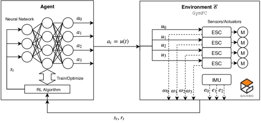
Figure 3$\cdot$1: RL architecture using the GymFC environment for training intelligent attitude flight controllers.

At each discrete time-step $t$, the agent receives an observation $x_{t}$ from the environments consisting of the angular velocity error of each axis $e=\Omega^{*}-\Omega$ and the angular velocity of each rotor $\omega_{i}$ which are obtained from the quadcopter’s emulated inertial measurement unit (IMU) and electronic speed controller (ESC) sensors respectively. These observations are in the continuous observation spaces $x_{t}\in\mathbb{R}^{(M+D)}$ where $D=3$ degrees of rotational freedom. Once the observation is received, the agent executes an action $a_{t}$ within $\mathcal{E}$. In return the agent receives a single numerical reward $r_{t}$ indicating the performance of this action. The action is also in a continuous action space $a_{t}\in\mathbb{R}^{M}$ and corresponds to the four control signals $u(t)$ sent to each ESC driving the attached motor . Because the agent is only receiving this sensor data it is unaware of the physical environment and the aircraft dynamics and therefore $\mathcal{E}$ is only partially observed by the agent. Motivated by [Mnih et al., 2013] we consider the state to be a sequence of the past observations and actions $s_{t}=x_{i},a_{i},\dots,a_{t-1},x_{t}$.

3.3 GymFCv1

In this section we describe our learning environment GymFCv1 for developing intelligent flight control systems using RL. The goal of the proposed environment is to allow the agent to learn attitude control of an aircraft with only the knowledge of the number of actuators. GymFCv1 includes both an episodic task and a continuous task. In an episodic task, the agent is required to learn a policy for responding to individual angular velocity commands. This allows the agents to learn the step response from rest for a given command, allowing its performance to be accurately measured. Episodic tasks however are not reflective of realistic flight conditions. For this reason, in a continuous task, pulses with random widths and amplitudes are continuously generated, and correspond to angular velocity set-points. The agent must respond accordingly and track the desired target over time. In Section 3.4 we evaluate our synthesized controllers via episodic tasks, but we have strong experimental evidence that training via episodic tasks produces controllers that behave correctly in continuous tasks as well (Section 3.4.3).

GymFCv1 has a multi-layer hierarchical architecture composed of three layers: (i) a digital twin layer, (ii) a communication layer, and (iii) an agent-environment interface layer. This design decision was made to clearly establish roles and allow layer implementations to change (e.g., to use a different simulator) without affecting other layers as long as the layer-to-layer interfaces remain intact. A high level overview of the environment architecture is illustrated in Figure 3$\cdot$2. We will now discuss in greater detail each layer with a bottom-up approach.

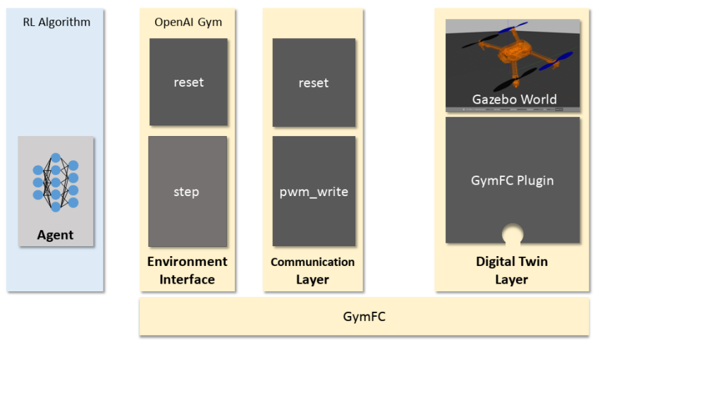
Figure 3$\cdot$2: Overview of GymFCv1 environment architecture.

3.3.1 Digital Twin Layer

At the heart of the learning environment is a high fidelity physics simulator which provides functionality and realism that is hard to achieve with an abstract mathematical model of the aircraft and environment. One of the primary design goals of GymFCv1 is to minimize the effort required to transfer a controller from the learning environment into the final platform. For this reason, the simulated environment exposes identical interfaces to actuators and sensors as they would exist in the physical world. In the ideal case the agent should not be able to distinguish between interaction with the simulated world (i.e., its digital twin) and its hardware counter part.

In a nutshell, the digital twin layer is defined by (i) the simulated world, and (ii) its interfaces to the above communication layer (see Figure 3$\cdot$2).

Simulated World The simulated world is constructed specifically for UAV attitude control in mind. The technique we developed allows attitude control to be accomplished independently of guidance and/or navigation control. This is achieved by fixing the center of mass of the aircraft to a ball joint in the world, allowing it to rotate freely in any direction, which would be impractical if not impossible to achieved in the real world due to gimbal lock and friction of such an apparatus. In this work the aircraft to be controlled in the environment is modeled off of the Iris quadcopter [iri, 2018] with a weight of 1.5 Kg, and 550 mm motor-to-motor distance. An illustration of the quadcopter in the environment is displayed in Figure 3$\cdot$3. Note during training Gazebo runs in headless mode without this user interface to increase simulation speed. This architecture however can be used with any multicopter as long as a digital twin can be constructed. Helicopters and multicopters represent excellent candidates for our setup because they can achieve a full range of rotations along all the three axes. This is typically not the case with fixed-wing aircraft. Our design can however be expanded to support fixed-wing by simulating airflow over the control surfaces for attitude control. Gazebo already integrates a set of tools for modelling lift and drag.

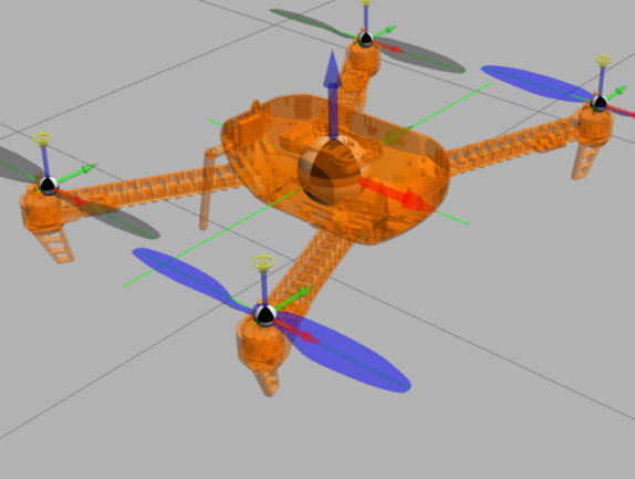
Figure 3$\cdot$3: The Iris quadcopter in Gazebo one meter above the ground. The body is transparent to show where the center of mass is linked as a ball joint to the world. Arrows represent the various joints used in the model.

Interface The digital twin layer provides two command interfaces to the communication layer: simulation reset and motor update. Simulation reset commands are supported by Gazebo’s API and are not part of our implementation. Motor updates are provided by a UDP server. We hereby discuss our approach to developing this interface.

In order to keep synchronicity between the simulated world and the controller of the digital twin, the pace at which simulation should progress is directly enforced. This is possible by controlling the simulator step-by-step. In our initial approach, Gazebo’s Google Protobuf [pro, 2018] API was used, with a specific message to progress by a single simulation step. By subscribing to status messages (which include the current simulation step) it is possible to determine when a step has completed and to ensure synchronization. However as we attempted to increase the rate of advertising step messages, we discovered that the rate of status messages is capped at 5 Hz. Such a limitation introduces a consistent bottleneck in the simulation/learning pipeline. Furthermore it was found that Gazebo silently drops messages it cannot process.

A set of important modifications were made to increase experiment throughput. The key idea was to allow motor update commands to directly drive the simulation clock. By default Gazebo comes pre-installed with an ArduPilot Arducopter [ard, 2018] plugin to receive motor updates through a UDP server. These motor updates are in the form of pulse width modulation (PWM) signals. At the same time, sensor readings from the inertial measurement unit (IMU) on board the aircraft is sent over a second UDP channel. Arducopter is an open source multicopter firmware and its plugin was developed to support SITL testing.

We derived our GymFC aircraft plugin from the Arducopter plugin with the following modifications (as well as those discussed in Section 3.3.2). Upon receiving a motor command, the motor forces are updated as normal but then a simulation step is executed. Sensor data is read and then sent back as a response to the client over the same UDP channel. In addition to the IMU sensor data we also simulate sensor data obtained from the electronic speed controller (ESC). The ESC provides the angular velocities of each rotor, which are relayed to the client too. Implementing our GymFC Plugin with this approach successfully allowed us to work around the limitations of the Google Protobuf API and increased step throughput by over 200 times.

3.3.2 Communication Layer

The communication layer is positioned in between the digital twin and the agent-environment interface. This layer manages the low-level communication channel to the aircraft and simulation control. The primary function of this layer is to export a high-level synchronized API to the higher layers for interacting with the digital twin which uses asynchronous communication protocols. This layer provides the commands pwm_write and reset to the agent-environment interface layer.

The function call pwm_write takes as input a vector of PWM values for each actuator, corresponding to the control input $u(t)$. These PWM values correspond to the same values that would be sent to an ESC on a physical UAV. The PWM values are translated to a normalized format expected by the GymFC Plugin, and then packed into a UDP packet for transmission to the GymFC Plugin UDP server. The communication layer blocks until a response is received from the GymFC Plugin, forcing synchronized writes for the above layers. The UDP reply is unpacked and returned in response.

During the learning process the simulated environment must be reset at the beginning of each learning episode. Ideally one could use the gz command line utility included with the Gazebo installation which is lightweight and does not require additional dependencies. Unfortunately there is a known socket handle leak [gzb, 2018] that causes Gazebo to crash if the command is issued more than the maximum number of open files allowed by the operating system. Given we are running thousands episodes during training this was not an option for us. Instead we opted to use the Google Protobuf interface so we did not have to deploy a patched version of the utility on our test servers. Because resets only occur at the beginning of a training session and are not in the critical processing loop, using the Google Protobuf API here is acceptable.

Upon start of the communication layer, a connection is established with the Google Protobuf API server and we subscribe to world statistics messages which includes the current simulation iteration. To reset the simulator, a world control message is advertised instructing the simulator to reset the simulation time. The communication layer blocks until it receives a world statistics message indicating the simulator has been reset and then returns back control to the agent-environment interface layer. Note the world control message is only resetting the simulation time, not the entire simulator (i.e., models and sensors). This is because we found that in some cases when a world control message was issued to perform a full reset the sensor data took a few additional iterations for reset. To ensure proper reset to the above layers this time reset message acts as a signalling mechanism to the GymFC Plugin. When the plugin detects a time reset has occurred it resets the whole simulator and most importantly steps the simulator until the sensor values have also reset ensuring above layers that when a new training session starts, reading sensor values accurately reflect the current state and not the previous state from stale values.

3.3.3 Environment Interface Layer

The topmost layer interfacing with the agent is the environment interface layer which implements the OpenAI Gym [Brockman et al., 2016] environment API. Each OpenAI Gym environment defines an observation space and an action space. These are used to inform the agent of the bounds to expect for environment observations and what are legal bounds for the action input, respectively. As previously mentioned in Section 3.2 GymFCv1 is in both the continuous observation space and action space domain. The state is of size $m\times(M+D)$ where $m$ is the memory size indicating the number of past observations; $M=4$ as we consider a four-motor configuration; and $D=3$ since each measurement is taken in the 3 dimensions. Each observation value is in $[-\infty:\infty]$. The action space is of size $M$ equivalent to the number of control actuators of the aircraft (i.e., four for a quadcopter), where each value is normalized between $[-1:1]$ to be compatible with most agents who squash their output using the hyperbolic tangent function.

GymFCv1 implements two primary OpenAI functions, namely reset and step. The reset function is called at the start of an episode to reset the environment and returns the initial environment state. This is also when the desired target angular velocity $\Omega^{*}$ or setpoint is computed. The setpoint is randomly sampled from a uniform distribution between $[\Omega_{min},\Omega_{max}]$. For the continuous task this is also set at a random interval of time. Selection of these bounds may refer to the desired operating region of the aircraft. Although it is highly unlikely during normal operation that a quadcopter will be expected to reach the majority of these target angular velocities, the intention of these tasks are to push and stress the performance of the aircraft.

The step function executes a single simulation step with the specified actions and returns to the agent the new state vector, together with a reward indicating how well the given action was performed. Reward engineering can be challenging. If careful design is not performed, the derived policy may not reflect what was originally intended. Recall from Section 3.2 that the reward is ultimately what shapes the policy. For this work, with the goal of establishing a baseline of accuracy, we develop a reward to reflect the current angular velocity error (i.e., $e=\Omega^{*}-\Omega$). In the future GymFCv1 will be expanded to include additional environments aiding in the development of more complex policies particularity to showcase the advantages of using RL to adapt and learn. We translate the current error $e_{t}$ at time $t$ into into a derived reward $r_{t}$ normalized between $[-1,0]$ as follows,

$$r_{t}=-clip\left(sum(|\Omega^{*}_{t}-\Omega_{t}|)/3\Omega_{max}\right)$$ (3.1)

where the $sum$ function sums the absolute value of the error of each axis, and the $clip$ function clips the result between the $[0,1]$ in cases where there is an overflow in the error. Since the reward is negative, it signifies a penalty, the agent maximizes the rewards (and thus minimizing error) overtime in order to track the target as accurately as possible. Rewards are normalized to provide standardization and stabilization during training [Karpathy, 2018].

Additionally we also experimented with a variety of other rewards. We found sparse binary rewards to give poor performance. We believe this to be due to complexity of quadcopter control. In the early stages of learning the agent explores its environment. However the event of randomly reaching the target angular velocity within some threshold was rare and thus did not provide the agent with enough information to converge. Conversely, we found that signalling at each timestep was best.

3.4 Evaluation

In this section we present our evaluation on the accuracy of studied NN-based attitude flight controllers trained with RL. To our knowledge, this is the first RL baseline conducted for quadcopter attitude control.

3.4.1 Setup

We evaluate the RL algorithms DDPG, TRPO, and PPO using the implementations in the OpenAI Baselines project [Dhariwal et al., 2017]. The goal of the OpenAI Baselines project is to establish a reference implementation of RL algorithms, providing baselines for researchers to compare approaches and build upon. Every algorithm is run with defaults except for the number of simulations steps which we increased to 10 million. For reference the hyperparameters can be found in Table 3.1, Table 3.2, and Table 3.3 for PPO, TRPO and DDPG respectively. The PPO, TRPO NN architectures have two hidden layers with 32 nodes each using hyperbolic tangent functions. The DDPG actor network has two hidden layers of 64 nodes using rectified linear units, while the output layer uses hyperbolic tangent functions. The DDPG critic layer also has the same internal structure however the output layer is unbounded.

Hyperparameter	Value
Horizon (T)	2048
Adam stepsize	$3\times 10^{-4}\times\rho$
Num. epochs	10
Minibatch size	64
Discount ($\gamma$)	0.99
GAE parameter ($\lambda$)	0.95

Table 3.1: PPO hyperparameters where $\rho$ is linearly annealed over the course of training from 1 to 0.

Hyperparameter	Value
Horizon	1024
Max KL-divergence	0.01
Value function learning rate	$1\times 10^{-3}$
Num. epochs	5
Discount ($\gamma$)	0.99
GAE parameter ($\lambda$)	0.98

Table 3.2: TRPO hyperparameters.

Hyperparameter	Value
Num. epochs	5000
Num. epochs per cycle	20
Num. rollout steps	100
Batch size	64
Noise type	adaptive-param_0.2
Actor learning rate	$1\times 10^{-4}$
Critic learning rate	$1\times 10^{-3}$
Discount ($\gamma$)	0.99

Table 3.3: DDPG hyperparameters.

The episodic task parameters were configured to run each episode for a maximum of 1 second of simulated time allowing enough time for the controller to respond to the command as well as additional time to identify if a steady state has been reached. The bounds the target angular velocity is sampled from is set to $\Omega_{min}=-5.24$ rad/s, $\Omega_{max}=5.24$ rad/s ($\pm$ 300 deg/s). These limits were constructed by examining PID’s performance to make sure we expressed physically feasible constraints. The max step size of the Gazebo simulator, which specifies the duration of each physics update step was set to 1 ms to develop highly accurate simulations. In other words, our physical world “evolved” at 1 kHz. Training and evaluations were run on Ubuntu 16.04 with an eight-core i7-7700 CPU and an NVIDIA GeForce GT 730 graphics card.

For our PID controller, we ported the mixing and SITL implementation from Betaflight [bet, 2018] to Python to be compatible with GymFCv1. The PID controller was first tuned using the classical Ziegler-Nichols method [Ziegler and Nichols, 1942] and then manually adjusted to improve performance of the step response sampled around the midpoint $\pm\Omega_{max}/2$. We obtained the following gains for each axis of rotation: $K_{\phi}=[2,10,0.005],K_{\theta}=[10,10,0.005],K_{\psi}=[4,50,0.0]$, where each vector contains to the $[K_{P},K_{I},K_{D}]$ (proportional, integrative, derivative) gains, respectively. Next we measured the distances between the arms of the quadcopter to calculate the mixer values for each motor $m_{i},i\in\{0,\ldots,3\}$. Each vector $m_{i}$ is of the form $m_{i}=[m_{(i,\phi)},m_{(i,\theta)},m_{(i,\psi)}]$, i.e., roll, pitch, and yaw (see Section 2.3). The final values were: $m_{0}=[-1.0,0.598,-1.0]$, $m_{1}=[-0.927,-0.598,1.0]$, $m_{2}=[1.0,0.598,1.0]$ and lastly $m_{3}=[0.927,-0.598,-1.0]$. The mix values and PID sums are then used to compute each motor signal $u_{i}$ according to Equation 2.7, where $\mathbf{T}=0$ for no additional throttle.

To evaluate and compare the accuracy of the different algorithms we used a set of metrics. First, we define “initial error” as the distance between the rest velocities and the current setpoint. A notion of progress toward the setpoint from rest can then be expressed as the percentage of the initial error that has been “corrected”. Correcting 0% of the initial error means that no progress has been made; while 100% indicates that the setpoint has been reached. Each metric value is independently computed for each axis. We hereby list our metrics. Success captures the number of experiments (in percentage) in which the controller eventually settles in an band within 90% an 110% of the initial error, i.e., $\pm 10\%$ from the setpoint. Failure captures the average percent error relative to the initial error after $t=500~{}ms$, for those experiments that do not make it in the $\pm 10\%$ error band. The latter metric quantifies the magnitude of unacceptable controller performance. The delay in the measurement ($t>500~{}ms$) is to exclude the rise regime. The underlying assumption is that a steady state is reached before $500~{}ms$. Rise is the average time in milliseconds it takes the controller to go from 10% to 90% of the initial error. Peak is the max achieved angular velocity represented as a percentage relative to the initial error. Values greater than 100% indicate overshoot, while values less than 100% represent undershoot. Error is the mean sum of the absolute value error of each episode in radians per second. This provides a generic metric for performance. Our last metric is Stability, which captures how stable the response is halfway through the simulation, i.e., at $t>500ms$. Stability is calculated by taking the linear regression of the angular velocities and reporting the slope of the calculated line. Systems that are unstable have a non-zero slope.

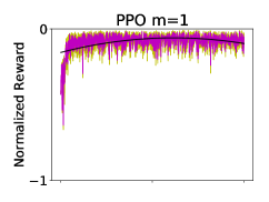
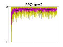
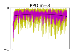
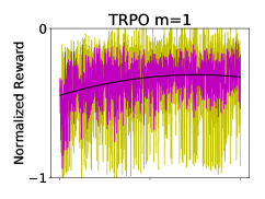
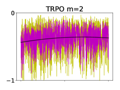
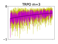
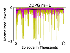
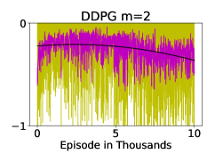
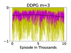
Figure 3$\cdot$4: Average normalized rewards shown in magenta received during training of 10,000 episodes (10 million steps) for each RL algorithm and memory $m$ sizes 1, 2 and 3. Plots share common $y$ and $x$ axis. Additionally, yellow represents the 95% confidence interval and the black line is a two degree polynomial added to illustrate the trend of the rewards over time.

Table 3.4: Rise time averages from 3,000 command inputs per configuration with 95% confidence.

		Rise (ms)
	$m$	$\phi$	$\theta$	$\psi$
PPO	1	65.9$\pm$2.4	94.1$\pm$4.3	73.4$\pm$2.7
	2	58.6$\pm$2.5	125.4$\pm$6.0	105.0$\pm$5.0
	3	101.5$\pm$5.0	128.8$\pm$5.8	79.2$\pm$3.3
TRPO	1	103.9$\pm$6.2	150.2$\pm$6.7	109.7$\pm$8.0
	2	161.3$\pm$6.9	162.7$\pm$7.0	108.4$\pm$9.6
	3	130.4$\pm$7.1	150.8$\pm$7.8	129.1$\pm$8.9
DDPG	1	68.2$\pm$3.7	100.0$\pm$5.4	79.0$\pm$5.4
	2	49.2$\pm$1.5	99.1$\pm$4.9	40.7$\pm$1.8
	3	85.3$\pm$5.9	124.3$\pm$7.2	105.1$\pm$8.6

Table 3.5: Peak averages from 3,000 command inputs per configuration with 95% confidence.

		Peak (%)
	$m$	$\phi$	$\theta$	$\psi$
PPO	1	113.8$\pm$2.2	107.7$\pm$2.2	128.1$\pm$4.3
	2	116.9$\pm$2.5	103.0$\pm$2.7	126.8$\pm$3.7
	3	108.9$\pm$2.2	94.2$\pm$5.3	119.8$\pm$2.7
TRPO	1	125.1$\pm$9.3	110.4$\pm$3.9	139.6$\pm$6.8
	2	100.1$\pm$5.1	144.2$\pm$13.8	101.7$\pm$5.4
	3	141.3$\pm$7.2	141.2$\pm$8.1	147.1$\pm$6.8
DDPG	1	133.1$\pm$7.8	116.6$\pm$7.9	146.4$\pm$7.5
	2	42.0$\pm$5.5	46.7$\pm$8.0	71.4$\pm$7.0
	3	101.0$\pm$8.2	158.6$\pm$21.0	120.5$\pm$7.0

Table 3.6: Error averages from 3,000 command inputs per configuration with 95% confidence.

		Error (rad/s)
	$m$	$\phi$	$\theta$	$\psi$
PPO	1	309.9$\pm$7.9	440.6$\pm$13.4	215.7$\pm$6.7
	2	305.2$\pm$7.9	674.5$\pm$19.1	261.3$\pm$7.6
	3	405.9$\pm$10.9	1403.8$\pm$58.4	274.4$\pm$5.3
TRPO	1	1644.5$\pm$52.1	929.0$\pm$25.6	1374.3$\pm$51.5
	2	1432.9$\pm$47.5	2375.6$\pm$84.0	1475.6$\pm$46.4
	3	1120.1$\pm$36.4	1200.7$\pm$34.3	824.0$\pm$30.1
DDPG	1	1201.4$\pm$42.4	1397.0$\pm$62.4	992.9$\pm$45.1
	2	2388.0$\pm$63.9	2607.5$\pm$72.2	1953.4$\pm$58.3
	3	1984.3$\pm$59.3	3280.8$\pm$98.7	1364.2$\pm$54.9

Table 3.7: Stability averages from 3,000 command inputs per configuration with 95% confidence.

		Stability
	$m$	$\phi$	$\theta$	$\psi$
PPO	1	0.0$\pm$0.0	0.0$\pm$0.0	0.0$\pm$0.0
	2	0.0$\pm$0.0	0.0$\pm$0.0	0.0$\pm$0.0
	3	0.0$\pm$0.0	0.0$\pm$0.0	0.0$\pm$0.0
TRPO	1	-0.4$\pm$0.1	-0.2$\pm$0.0	-0.1$\pm$0.0
	2	0.1$\pm$0.0	0.4$\pm$0.0	-0.1$\pm$0.0
	3	0.1$\pm$0.0	-0.1$\pm$0.1	-0.1$\pm$0.0
DDPG	1	0.0$\pm$0.0	-0.1$\pm$0.0	0.1$\pm$0.0
	2	-0.1$\pm$0.0	-0.1$\pm$0.0	-0.0$\pm$0.0
	3	0.0$\pm$0.1	0.2$\pm$0.1	0.0$\pm$0.0

Table 3.8: Success and Failure results for considered algorithms. The row highlighted in blue refers to our best-performing learning agent PPO, while the rows highlighted in yellow correspond to the best agents for the other two algorithms.

		Success (%)			Failure (%)
	$m$	$\phi$	$\theta$	$\psi$	$\phi$	$\theta$	$\psi$
PPO	1	99.8$\pm$0.3	100.0$\pm$0.0	100.0$\pm$0.0	0.1$\pm$0.1	0.0$\pm$0.0	0.0$\pm$0.0
	2	100.0$\pm$0.0	53.3$\pm$3.1	99.8$\pm$0.3	0.0$\pm$0.0	20.0$\pm$2.4	0.0$\pm$0.0
	3	98.7$\pm$0.7	74.7$\pm$2.7	99.3$\pm$0.5	0.4$\pm$0.2	5.4$\pm$0.7	0.2$\pm$0.2
TRPO	1	32.8$\pm$2.9	59.0$\pm$3.0	87.4$\pm$2.1	72.5$\pm$10.6	17.4$\pm$3.7	9.4$\pm$2.6
	2	19.7$\pm$2.5	48.2$\pm$3.1	56.9$\pm$3.1	76.6$\pm$5.0	43.0$\pm$6.5	38.6$\pm$7.0
	3	96.8$\pm$1.1	60.8$\pm$3.0	73.2$\pm$2.7	1.5$\pm$0.8	20.6$\pm$4.1	20.6$\pm$3.4
DDPG	1	84.1$\pm$2.3	52.5$\pm$3.1	90.4$\pm$1.8	11.1$\pm$2.2	41.1$\pm$5.5	4.6$\pm$1.0
	2	26.6$\pm$2.7	26.1$\pm$2.7	50.2$\pm$3.1	82.7$\pm$8.5	112.2$\pm$12.9	59.7$\pm$7.5
	3	39.2$\pm$3.0	44.8$\pm$3.1	60.7$\pm$3.0	52.0$\pm$6.4	101.8$\pm$13.0	33.9$\pm$3.4
PID		100.0$\pm$0.0	100.0$\pm$0.0	100.0$\pm$0.0	0.0$\pm$0.0	0.0$\pm$0.0	0.0$\pm$0.0

Table 3.9: RL rise time evaluation compared to PID of best-performing agent. Values reported are the average of 1,000 command inputs with 95% confidence. PPO $m=1$ highlighted in blue outperforms all other agents, including PID control. Metrics highlighted in red for PID control are outpreformed by the PPO agent.

		Rise (ms)
	$m$	$\phi$	$\theta$	$\psi$
PPO	1	66.6$\pm$3.2	70.8$\pm$3.6	72.9$\pm$3.7
	2	64.4$\pm$3.6	102.8$\pm$6.7	148.2$\pm$7.9
	3	97.9$\pm$5.5	121.9$\pm$7.2	79.5$\pm$3.7
TRPO	1	119.9$\pm$8.8	149.0$\pm$10.6	103.9$\pm$9.8
	2	108.0$\pm$8.3	157.1$\pm$9.9	47.3$\pm$6.5
	3	115.2$\pm$9.5	156.6$\pm$12.7	176.1$\pm$15.5
DDPG	1	64.7$\pm$5.2	118.9$\pm$8.5	51.0$\pm$4.8
	2	49.2$\pm$2.1	99.1$\pm$6.9	40.7$\pm$2.5
	3	73.7$\pm$8.4	172.9$\pm$12.0	141.5$\pm$14.5
PID		79.0$\pm$3.5	99.8$\pm$5.0	67.7$\pm$2.3

Table 3.10: RL peak angular velocity percentage evaluation compared to PID of best-performing agent. Values reported are the average of 1,000 command inputs with 95% confidence. PPO $m=1$ highlighted in blue outperforms all other agents, including PID control. Metrics highlighted in red for PID control are outpreformed by the PPO agent.

		Peak (%)
	$m$	$\phi$	$\theta$	$\psi$
PPO	1	112.6$\pm$3.0	109.4$\pm$2.4	127.0$\pm$6.2
	2	118.4$\pm$4.3	104.2$\pm$4.7	124.2$\pm$3.4
	3	111.4$\pm$3.4	111.1$\pm$4.2	120.8$\pm$4.2
TRPO	1	103.0$\pm$11.0	117.4$\pm$5.8	142.8$\pm$6.5
	2	69.4$\pm$7.4	117.7$\pm$9.2	126.5$\pm$7.2
	3	153.5$\pm$8.1	123.3$\pm$6.9	148.8$\pm$11.2
DDPG	1	165.6$\pm$11.6	135.4$\pm$12.8	150.8$\pm$6.2
	2	84.0$\pm$10.4	93.5$\pm$15.4	142.7$\pm$12.5
	3	103.7$\pm$11.5	126.5$\pm$17.8	119.6$\pm$8.2
PID		136.9$\pm$4.8	112.7$\pm$1.6	135.1$\pm$3.3

Table 3.11: RL error evaluation compared to PID of best-performing agent. Values reported are the average of 1,000 command inputs with 95% confidence. PPO $m=1$ highlighted in blue outperforms all other agents, including PID control. Metrics highlighted in red for PID control are outpreformed by the PPO agent.

		Error (rad/s)
	$m$	$\phi$	$\theta$	$\psi$
PPO	1	317.0$\pm$11.0	326.3$\pm$13.2	217.5$\pm$9.1
	2	329.4$\pm$12.3	815.3$\pm$31.4	320.6$\pm$11.5
	3	396.7$\pm$14.7	540.6$\pm$22.6	237.1$\pm$8.0
TRPO	1	1965.2$\pm$90.5	930.5$\pm$38.4	713.7$\pm$34.4
	2	2020.2$\pm$71.9	1316.2$\pm$49.0	964.0$\pm$31.2
	3	643.5$\pm$20.5	895.0$\pm$42.8	1108.9$\pm$44.5
DDPG	1	929.1$\pm$39.9	1490.3$\pm$83.0	485.3$\pm$25.4
	2	2074.1$\pm$86.4	2498.8$\pm$109.8	1336.9$\pm$50.1
	3	1585.4$\pm$81.4	2401.3$\pm$109.8	1199.0$\pm$74.0
PID		416.1$\pm$20.4	269.6$\pm$11.9	245.1$\pm$11.5

Table 3.12: RL stability evaluation compared to PID of best-performing agent. Values reported are the average of 1,000 command inputs with 95% confidence. PPO $m=1$ highlighted in blue outperforms all other agents, including PID control. Metrics highlighted in red for PID control are outpreformed by the PPO agent.

		Stability
	$m$	$\phi$	$\theta$	$\psi$
PPO	1	0.0$\pm$0.0	0.0$\pm$0.0	0.0$\pm$0.0
	2	0.0$\pm$0.0	0.0$\pm$0.0	0.0$\pm$0.0
	3	0.0$\pm$0.0	0.0$\pm$0.0	0.0$\pm$0.0
TRPO	1	0.7$\pm$0.1	0.3$\pm$0.0	0.0$\pm$0.0
	2	0.1$\pm$0.1	0.5$\pm$0.1	0.0$\pm$0.0
	3	0.1$\pm$0.0	0.0$\pm$0.0	0.0$\pm$0.0
DDPG	1	0.1$\pm$0.1	-0.2$\pm$0.1	0.1$\pm$0.0
	2	-0.1$\pm$0.0	-0.2$\pm$0.1	-0.0$\pm$0.0
	3	-0.1$\pm$0.1	-0.2$\pm$0.1	0.1$\pm$0.0
PID		0.0$\pm$0.0	0.0$\pm$0.0	0.0$\pm$0.0

3.4.2 Results

Each learning agent was trained with an RL algorithm for a total of 10 million simulation steps, equivalent to 10,000 episodes or about 2.7 simulation hours. The agents configuration is defined as the RL algorithm used for training and its memory size $m$. Training for DDPG took approximately 33 hours, while PPO and TRPO took approximately 9 hours and 13 hours respectively. The average sum of rewards for each episode is normalized between $[-1,0]$ and displayed in Figure 3$\cdot$4. This computed average in magenta is from 3 independently trained agents with the same configuration, while the 95% confidence is shown in yellow. Additionally we have added a two degree polynomial in black fit to the data to illustrate the reward trend over time. Training results show clearly that PPO converges consistently compared to TRPO and DDPG, and overall PPO accumulates higher rewards. What is also interesting and counter-intuitive is that the larger memory size actually decreases convergence and stability among all trained algorithms. Recall from Section 2.4.1 that RL algorithms learn a policy to map states to action. A reason for the decrease in convergence could be attributed to the state space increasing causing the RL algorithm to take longer to learn the mapping to the optimal action. As part of our future work, we plan to investigate using separate memory sizes for the error and rotor velocity to decrease the state space. Additionally increasing the size of the NN could compensate for the increase in state space. Reward gains during training of TRPO and DDPG are quite inconsistent with large confidence intervals. Although performance for DDPG $m=1$ looks promising, upon further investigation into the large confidence interval we found this was due to the algorithm completely failing to respond to certain command inputs thus questioning whether the algorithm has learned the underlying flight dynamics (this is emphasized later in Table 3.8).

In the future we plan to investigate methods to decrease training times by addressing challenges C2 and C3. Specific to C2 to support a large range of aircraft, we will explore whether we can construct a generic NN taught general flight dynamics (Section 2.2) which will provide a baseline to extend training to create intelligent controllers unique to an aircraft (otherwise known as domain adaptation [Blitzer et al., 2008]). Additionally considering C3 we will experiment with developing more expressive reward functions to decrease training times.

Each trained agent was then evaluated on 1,000 never before seen command inputs in an episodic task. Since there are 3 agents per configuration, each configuration was evaluated over a total of 3,000 episodes. The average performance metrics are reported in Table 3.4 for Rise, Table 3.5 for Peak, Table 3.6 for Error and Table 3.7 for Stability. Results show that the agent trained with PPO outperforms TRPO and DDPG in every measurement. In fact, PPO is the only one that is able to achieve stability (for every $m$), while all other agents have at least one axis where the Stability metric is non-zero.

Next the best performing agent for each algorithm and memory size is compared to the PID controller. The best agent was selected based on the lowest sum of errors of all three axis reported by the Error metric. The Success and Failure metrics are compared in Table 3.8. Results show that agents trained with PPO would be the only ones good enough for flight, with a success rate close to perfect, and where the roll failure of $0.2\%$ is only off by about $0.1\%$ from the setpoint. However the best trained agents for TRPO and DDPG are often significantly far away from the desired angular velocity. For example TRPO’s best agent, $39.2\%$ (60.8% success, see Table 3.8) of the time does not reach the desired pitch target with upwards of a $20\%$ error from the setpoint.

Next we provide our thorough analysis comparing the best agents in Table 3.9 for Rise, Table 3.10 for Peak, Table 3.11 for Error and Table 3.12 for Stability. We have found that RL agents trained with PPO using $m=1$ provide performance and accuracy exceeding that of our PID controller in regards to rise time, peak velocities achieved, and total error. What is interesting is that usually a fast rise time could cause overshoot however the PPO agent has on average a faster rise time and less overshoot. This is most likely explained by the faster switching and oscillations causes in the PWM control signal output of the PPO controller, allowing it to compensate quicker than PID control. However if transferred to the real world, the addition of these oscillations could be problematic. Both PPO and PID reach a stable state measured halfway through the simulation.

To illustrate the performance of each of the best agents a random simulation is sampled and the step response for each attitude command is displayed in Figure 3$\cdot$5 along with the target angular velocity to achieve $\Omega^{*}$. All algorithms reach some steady state however only PPO and PID do so within the error band indicated by the dashed red lines. TRPO and DDPG have extreme oscillations in both the roll and yaw axis, which would cause instability during flight. In this particular example we can observe PID to perform better with a 19% decrease in error compared to PPO, most visibly in yaw control. However globally speaking, in terms of error, PPO has shown to be a more accurate attitude controller.

To highlight the performance and accuracy of the PPO agent we sample another simulation and show the step response and also the PWM control signals generated by each controller in Figure 3$\cdot$6. In this figure we can see the PPO agent has exceptional tracking capabilities of the desired attitude. Compared to PID, the PPO controller has a 44% decrease in error. The PPO agent has a 2.25 times faster rise time on the roll axis, 2.5 times faster on the pitch axis and 1.15 time faster on the yaw axis. Furthermore the PID controller experiences slight overshoot in both the roll and yaw axis while the PPO agent does not. In regards to the control output, the PID controller exerts more power to motor three but then motor values eventually level off while the PPO control signal oscillates comparably more.

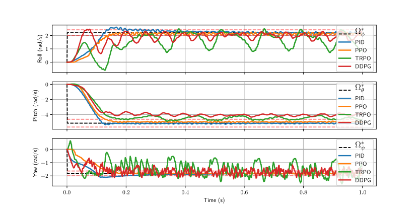
Figure 3$\cdot$5: Step response of best trained RL agents compared to PID. Target angular velocity is $\Omega^{*}=[2.20,-5.14,-1.81]$ rad/s shown by dashed black line. Error bars $\pm$10% of initial error from $\Omega^{*}$ are shown in dashed red.

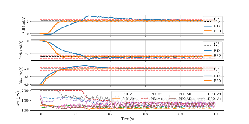
Figure 3$\cdot$6: Step response and PWM motor signals in microseconds ($\mu$s) of the best trained PPO agent compared to PID. Target angular velocity is $\Omega^{*}=[2.11,-1.26,5.00]$ rad/s shown by dashed black line. Error bars $\pm$10% of initial error from $\Omega^{*}$ are shown in dashed red.

3.4.3 Continuous Task Evaluation

In this section we briefly expand on our findings that show that even if agents are trained through episodic tasks their performance transfers to continuous tasks without the need for additional training. Figure 3$\cdot$7 shows that an agent trained with PPO using episodic tasks has exceptional performance when evaluated in a continuous task. Figure 3$\cdot$8 is a close up of another continuous task sample showing the details of the tracking and corresponding motor output. These results are quite remarkable as they suggest that training with episodic tasks is sufficient for developing intelligent attitude flight controller systems capable of operating in a continuous environment. In Figure 3$\cdot$9 another continuous task is sampled and the PPO agent is compared to a PID agent. The performance evaluation shows the PPO agent to have 22% decrease in overall error in comparison to the PID agent.

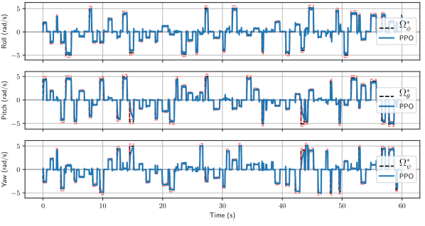
Figure 3$\cdot$7: Performance of PPO agent trained with episodic tasks but evaluated using a continuous task for a duration of 60 seconds. The time in seconds at which a new command is issued is randomly sampled from the interval $[0.1,1]$ and each issued command is maintained for a random duration also sampled from $[0.1,1]$. Desired angular velocity is specified by the black line while the red line is the attitude tracked by the agent.

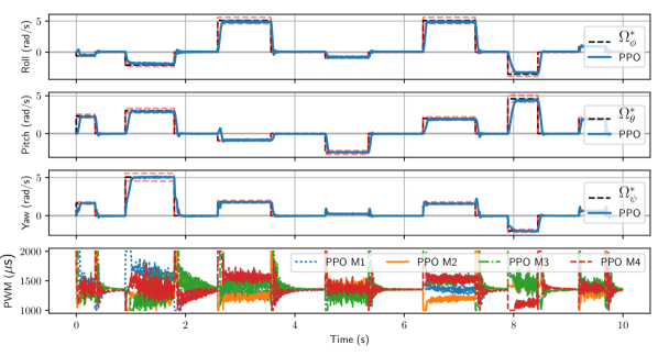
Figure 3$\cdot$8: Close up of continuous task results for PPO agent with PWM values.

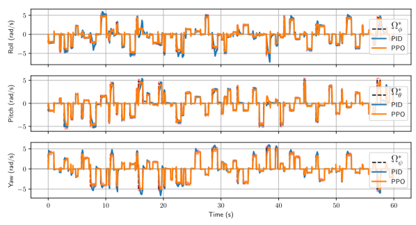
Figure 3$\cdot$9: Response comparison of a PID and PPO agent evaluated in continuous task environment. The PPO agent, however, is only trained using episodic tasks.

3.5 Future Work and Conclusion

In this chapter we presented our RL training environment GymFCv1 for developing intelligent attitude controllers for UAVs and addressed in-depth C1: Precision and Accuracy, which identifies if NNs trained with RL can produce accurate attitude controllers. We placed an emphasis on digital twinning concepts to allow transferability to real hardware. We used GymFCv1 to evaluate the performance of state-of-the-art RL algorithms PPO, TRPO and DDPG to identify if they are appropriate to synthesize high-precision attitude flight controllers. Our results highlight that: (i) RL can train accurate attitude controllers; and (ii) that those trained with PPO outperformed a fully tuned PID controller on almost every metric. It is important to note that although our analysis found our TRPO and DDPG policies to be insufficient in providing stable flight we did not perform any hyperparameter tuning in this work. Thus in future work further benchmarking will be required to discover the true capabilities and potential of these other algorithms.

Although we base our evaluation on results obtained in episodic tasks, we found that trained agents were able to perform exceptionally well also in continuous tasks without retraining (Section 3.4.3). This suggests that training using episodic tasks is sufficient for developing intelligent attitude controllers. The results presented in this work can be considered as a first milestone and a good motivation to further inspect the boundaries of RL for flight control.

With this premise, we plan to develop our future work along three main avenues. On the one hand, we plan to investigate C2: Robustness and Adaptation and C3: Reward Engineering to harness the true power of RL’s ability to adapt and learn in environments with dynamic properties (e.g., wind, variable payload, system damage and failure). On the other hand we intend to transfer our trained agents onto a real aircraft to evaluate their live performance including timing and memory analysis of the NN. This will allow us to define the minimum hardware specifications required to use NN attitude control. Furthermore, we plan to expand GymFCv1 to support other aircraft such as fixed wing, while continuing to increase the realism of the simulated environment by improving the accuracy of our digital twins.

Chapter 4 Neuroflight: Next Generation Flight Control Firmware

Recently there has been explosive growth in user-level applications developed for UAVs. However little innovation has been made to the UAV’s low-level attitude flight controller which still predominantly uses classic PID control. Although PID control has proven to be sufficient for a variety of applications, it falls short in dynamic flight conditions and environments (e.g., in the presence of wind, payload changes and voltage sags). In these cases, more sophisticated control strategies are necessary, that are able to adapt and learn. The use of NNs for flight control (i.e., neuro-flight control) has been actively researched for decades to overcome limitations in other control algorithms such as PID control. However the vast majority of research has focused on developing autonomous neuro-flight controller autopilots capable of tracking trajectories [Shepherd III and Tumer, 2010, Nicol et al., 2008, Dierks and Jagannathan, 2010, Bagnell and Schneider, 2001, Kim et al., 2004, Abbeel et al., 2007, Hwangbo et al., 2017, dos Santos et al., 2012].

In Chapter 3 we introduced our OpenAI gym environment GymFCv1. Via GymFCv1 it is possible to train NNs attitude control of a quadcopter in simulation using RL. Neuro-flight controllers trained with PPO [Schulman et al., 2017] were shown to exceed the performance of a PID controller. Nonetheless the attitude neuro-flight controllers were not validated in the real world, thus it remained as an open question if the NNs trained in GymFCv1 are capable of flight. As such, this chapter makes the following contributions:

• We introduce Neuroflight, the first open source neuro-flight controller firmware for multi-rotors and fixed wing aircraft. The NN embedded in Neuroflight replaces attitude control and motor mixing commonly found in traditional flight control firmwares (Section 4.2).

• To train neuro-flight controllers capable of stable flight in the real world we introduce GymFCv1.5, a modified environment addressing several challenges in making the transition from simulation to reality (Section 4.3).

• We propose a toolchain for compiling a trained NN to run on embedded hardware. To our knowledge this is the first work that consolidates a neuro-flight attitude controller on a microcontroller, rather than a multi-purpose onboard computer, thus allowing deployment on lightweight micro-UAVs (Section 4.4).

• Lastly, we provide an evaluation showing the NN can execute at over 2kHz on an Arm Cortex-M7 processor and flight tests demonstrate that a quadcopter running Neuroflight can achieve stable flight and execute aerobatic maneuvers such as rolls, flips, and the Split-S (Section 4.5). Source code for the project can be found at [Koch, 2018b] and videos of our test flights can be viewed at [Koch, 2018c].

The goal of this work is to provide the community with a stable platform to innovate and advance development of neuro-flight control design for UAVs, and to take a step towards making neuro-flight controllers mainstream. In the future we hope to establish NN powered attitude control as a convenient alternative to classic PID control for UAVs operating in harsh environments or that require particularly competitive set point tracking performance (e.g., drone racing).

4.1 Background and Related Work

Over time there has been a number of successes transferring controllers trained with RL to multicopters. This includes helicopters [Bagnell and Schneider, 2001, Kim et al., 2004, Abbeel et al., 2007] and quadcopters [Hwangbo et al., 2017, dos Santos et al., 2012]. Unfortunately none of these works have published any code thereby making it difficult to reproduce results and to build on top of their research. Furthermore evaluations are only in respect to the accuracy of position therefore it is still unknown how well attitude is controlled. Of the open source flight control firmwares currently available, every single one uses PID control [Ebeid et al., 2018].

In regards to methods and techniques for transferring trained policies to hardware, these are neglected in the helicopter control literature  [Bagnell and Schneider, 2001, Kim et al., 2004, Abbeel et al., 2007]. Given the resource constrained hardware onboard a quadcopter, hardware details are more commonly discussed, however strategies for policy transfer are still lagging behind. A common strategy for executing high-level navigation tasks is to use a separate companion (compute) board which computes the desired attitude commands and sends them over a serial connection to an off-the-shelf flight controller. For example the default configuration of the Intel Aero [int, 2019] uses an Intel compute board which communicates with a microcontroller running PX4. Previous research has used companion boards for onboard computation of RL controllers. In [Hwangbo et al., 2017] an Intel computer stick is used for the RL controller which outputs the desired motor thrust values. These are then provided as input to a software library for interfacing over serial to the separate flight control board. In [Palossi et al., 2019] the authors present an impressive vision based navigation system using an RL controller for the Crazyflie quadcopter. A companion board executes the NN and interfaces with the Crazyflie flight controller over the serial peripheral interface (SPI). Additionally this work provides an extensive evaluation of the architecture required to successfully perform vision navigation in such a resource constrained hardware environment.

To reduce weight and increase communication throughput a single control board should be used. Work by [Molchanov et al., 2019] executes their policy directly on the flight controller for a Crazyflie quadcopter. Nonetheless aircraft state estimation is offloaded to a ground station. Using a postprocessing stage after policy training, the network parameters from the trained model are extracted and compiled into a C function to be linked into the Crazyflie’s flight control firmware.

Developing a generic all-in-one flight control board capable of complex navigation tasks is challenging due to timing guarantees of time sensitive tasks. Advances made by [Cheng et al., 2018] have ported the flight control firmware Cleanflight [cle, 2018] to run within a real-time operating system. Their analysis on the Intel Aero compute board shows their approach is able to bound end-to-end latencies from sensor input to motor output.

4.2 Neuroflight Overview

Neuroflight is a fork of Betaflight version 3.3.3 [bet, 2018], a high performance flight controller firmware used extensively in first-person-view (FPV) multicopter racing. Internally Betaflight uses a two-degree-of-freedom PID controller (not to be confused with rotational degrees-of-freedom) for attitude control and includes other enhancements such as gain scheduling for increased stability when battery voltage is low and throttle is high. Betaflight runs on a wide variety of flight controller hardware based on the Arm Cortex-M family of microcontrollers. Flight control tasks are scheduled using a non-preemptive cooperative scheduler. The main PID controller task consists of multiple subtasks, including: (1) reading the remote control (RC) command for the desired angular velocity, (2) reading and filtering the angular velocity from the onboard gyroscope sensor, (3) evaluating the PID controller, (4) applying motor mixing to the PID output to account for asymmetries in the motor locations (see Section 2.3 for further details on mixing), and (5) writing the motor control signals to the ESCs.

Neuroflight replaces Betaflight’s PID controller task with a neuro-flight controller task. This task uses a single NN for attitude control and motor mixing. The architecture of Neuroflight decouples the NN from the rest of the firmware allowing the NN to be trained and compiled independently. An overview of the architecture is illustrated in Fig. 4$\cdot$1. The compiled NN is then later linked into Neuroflight to produce a firmware image for the target flight controller hardware.

To Neuroflight, the NN appears to be a generic function $y(t)=f(x(t))$. The input is $x(t)=[e(t),\Delta e(t)]$ where $\Delta e(t)=e(t)-e(t-1)$. The output $y(t)=[y_{0},\dots,y_{M-1}]$ where $M$ is the number of aircraft actuators to be controlled and $y_{i}\in[0,1]$ is the control signal representing the percent power to be applied to the $i^{th}$ actuator. This output representation is protocol agnostic and is not compatible with NNs trained with GymFCv1 from Chapter 3 whose output is the PWM to be applied to the actuator. PWM is seldomly used in high performance flight control firmware and has been replaced by digital protocols such as DShot for improved accuracy and speed [bet, 2018].

At time $t$, the NN inputs are resolved; $\Omega^{*}(t)$ is read from the RX serial port which is either connected to a radio receiver in the case of manual flight or an onboard companion computer operating as an autopilot in the case of autonomous flight, and $\Omega(t)$ is read from the gyroscope sensor. The NN is then evaluated to obtain the control signal outputs $y(t)$. However the NN has no concept of thrust ($\mathbf{T}$), therefore to achieve translational movement the thrust command must be mixed into the NN output to produce the final control signal output to the ESC, $u(t)$. The logic of throttle mixing is to uniformly apply additional power across all motors proportional to the available range in the NN output, while giving priority to achieving $\Omega^{*}(t)$. This approach does make the assumption the performance of each motor is identical, which may not always be the case. If any output value is over saturated (i.e., $\exists y_{i}(t):y_{i}(t)\geq 1$) no additional throttle will be added. The input throttle value is scaled depending on the available output range to obtain the actual throttle value:

$$\widehat{\mathbf{T}}(t)=\mathbf{T}(t)\left(1-\mathrm{max}_{i}\{y_{i}(t)\}\right)$$ (4.1)

where the function $\mathrm{max}$ returns the max value from the NN output. The readjusted throttle value is then proportionally added to each NN output to form the final control signal output:

$$u_{i}(t)=\widehat{\mathbf{T}}(t)+y_{i}(t).$$ (4.2)

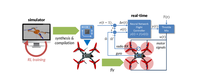
Figure 4$\cdot$1: Overview of the Neuroflight architecture.

4.3 GymFCv1.5

In this section we discuss the enhancements made to GymFCv1 to create GymFCv1.5. These changes primarily consist of a new state representation and reward system.

4.3.1 State Representation

GymFCv1 returns the state $x(t)=(e(t),\omega(t))$ to the agent at each time step. However not all UAVs have the sensors to measure motor velocity $\omega(t)$ as this typically involves digital ESC protocols. Even in an aircraft with compatible hardware, including the motor velocity as an input to the NN introduces additional challenges. This is because a NN trained on RPMs does not easily transfer from simulation to the real world, unless an accurate propulsion subsystem model is available for the digital twin. A mismatch between the physical propulsion system (i.e., motor/propeller combination) and the digital twin will result in the inability to achieve stable flight. Developing an accurate motor models is time-consuming and expensive. Specialized equipment is required to capture the relations between voltage, power consumption, temperature, rotor velocity, torque, and thrust.

To address these issues we investigated training using alternative environment states that do not rely on any specific characteristic of the motor(s). We posited that reducing the entire state to just angular velocity errors would carry enough information for the NN to achieve stable flight. At the same time, we expected that the obtained NN would transfer well to the real aircraft. Thus, our NN is trained by replacing $\omega(t)$ with the error differences $\Delta e(t)$. To identify the performance impact of this design choice, we trained two NNs. A first NN was trained with $\omega(t)$ in input. Its behavior was compared to a second NN trained in an environment that provides $\Delta e(t)$ instead. Both NNs were trained with PPO using hyperparameters from [Koch et al., 2019b] for 10 million steps. After training, each NN was validated against 10 never before seen random target angular velocities. Results show the NN trained in an environment with,

$$x(t)=(e(t),\Delta e(t))$$ (4.3)

experienced on average 45.07% less error with only an increase of 3.41% in its control signal outputs.

In RL the interaction between the agent and the environment can be formally modeled as a Markov Decision Process (MDP) in which the probability that the agent transitions to the next state depends on its current state and action to be taken. The behavior of the agent is defined by its policy which is essentially a mapping of states to actions. There may be multiple different state representations that are able to map to actions resulting in similar performance. For instance, it emerged from our experiments that using a history of errors as input to the NN also led to satisfactory performance. This approach has the disadvantage of requiring a state history table to be maintained, which ultimately made the approach less desirable.

The intuition why a state representation comprised of only angular velocity errors works can be summarized as follows. First, note that a PD controller (a PID controller with the integrative gain set to zero) is also a function computed over the angular velocity error. Because an NN is essentially a universal approximator, the expectation is that the NN would also be able to find a suitable control strategy based on these same inputs.

However, modifying the environment state alone is not enough to achieve stable flight. The RL task also needs to be adjusted. Training using episodic tasks, in which the aircraft is at rest and must reach an angular velocity never exposes the agent to scenarios in which the quadcopter must return to still from some random angular velocity. With the new state input consisting of the previous state, this is a significant difference from GymFCv1 which only uses the current state. For this purpose, a continuous task is constructed to mimic real flight, continually issuing commands. This task randomly samples a command and sets the target angular velocity to this command for a random amount of time. This command is then followed by an idle (i.e., $\Omega^{*}=[0,0,0]$) command to return the aircraft to still for a random amount of time. This is repeated until a max simulation time is reached.

4.3.2 Reward System

Reward engineering is a particularly difficult problem. As reward systems increase in complexity, they may present unintended side affects resulting in the agent behaving in an unexpected manner.

GymFCv1.5 reinforces stable flight behavior through our reward system defined as:

$$r=r_{e}+r_{y}+r_{\Delta}.$$ (4.4)

The agent is penalized for its angular velocity error, similar to GymFCv1, along each axis with:

$$r_{e}=-(e_{\phi}^{2}+e_{\theta}^{2}+e_{\psi}^{2}).$$ (4.5)

However we have identified the remaining two variables in the reward system as critical for transferability to the real world and achieving stable flight. Both rewards are a function of the agents control output. First $r_{y}$ rewards the agent for minimizing the control output, and next, $r_{\Delta}$ rewards the agent for minimizing oscillations.

The rewards as a function of the control signal are able to aid in the transferability by compensating for limitations in the training environment and unmodelled dynamics in the motor model.

Minimizing Output Oscillations. In the real world high frequency oscillations in the control output can damage motors. Rapid switching of the control output causes the ESC to rapidly change the angular velocity of the motor drawing excessive current into the motor windings. The increase in current causes high temperatures which can lead to the insulation of the motor wires to fail. Once the motor wires are exposed they will produce a short and “burn out” the motor.

The reward system used by GymFCv1 is strictly a function of the angular velocity error. This is inadequate in developing neuro-flight controllers that can be used in the real world. Essentially this produces controllers that closely resemble the behavior of an over-tuned PID controller. The controller is stuck in a state in which it is always correcting itself, leading to output oscillation.

In order to construct networks that produce smooth control signal outputs, the control signal output must be introduced into the reward system. This turned out to be quite challenging. Ultimately we were able to construct NNs outputting stable control outputs with the inclusion of the following reward:

$$r_{\Delta}=\beta\sum_{i=0}^{N-1}\text{max}\{0,\Delta y_{\text{max}}-\left(\Delta y_{i}\right)^{2}\}.$$ (4.6)

This reward is only applied if the absolute angular velocity error for every axis is less than some threshold (i.e., the error band). This allows the agent to be signaled by $r_{e}$ to reach the target without the influence from this reward. Maximizing $r_{\Delta}$ will drive the agent’s change in output to zero when in the error band. To derive $r_{\Delta}$, the change in the control output $y_{i}$ from the previous simulation step is squared to magnify the effect. This is then subtracted from a constant $\Delta y_{\text{max}}$ defining an upper bound for the change in the control output. The max function then forces a positive reward, therefore if $(\Delta y_{i})^{2}$ exceeds the limit no reward will be given. The rewards for each control output $N-1$ are summed and then scaled by a constant $\beta$, where $\beta>0$. Using the same training and validation procedure previously discussed, we found a NN trained in GymFCv1.5 compared to GymFCv1 resulted in a 87.95% decrease in $\Delta y$.

Minimizing Control Signal Output Values. Recall from Section 3.3.1, that the GymFCv1 environment fixes the aircraft to the simulation world about its center of mass, allowing it to only perform rotational movements. Due to this constraint the agent can achieve $\Omega^{*}$ with a number of different control signal outputs (e.g., when $\Omega^{*}=[0,0,0]$ this can be achieved as long as $y_{0}\equiv y_{1}\equiv y_{2}\equiv y_{3}$). However this poses a significant problem when transferred to the real world as an aircraft is not fixed about its center of mass. Any additional power to the motors will result in an unexpected change in translational movement. This is immediately evident when arming the quadcopter which should remain idle until RC commands are received. At idle, the power output (typically  4% of the throttle value) must not result in any translational movement. Another byproduct of inefficient control signals is a decreased throttle range (Section 4.2). Therefore it is desirable to have the NN control signals minimized while still maintaining the desired angular velocity. In order to teach the agent to minimize control outputs we introduce the reward function:

$$r_{y}=\alpha\left(1-\bar{y}\right)$$ (4.7)

providing the agent a positive reward as the output decreases. Since $y_{i}\leq 1$ we first compute the average output $\bar{y}$. Next $1-\bar{y}$ is calculated as a positive reward for low output usage which is scaled by a constant $\alpha$, where $\alpha>0$. NNs trained using this reward experience on average a 90.56% decrease in their control signal output.

Challenges and Lessons Learned. The fundamental challenge we faced was managing high amplitude oscillations in the control signal. In stochastic continuous control problems it is standard for the network to output the mean from a Gaussian distribution [Schulman et al., 2017, Chou et al., 2017]. However this poses problems for control tasks with bounded outputs such as flight control. The typical strategy is to clip the output to the target bounds yet we have observed this to significantly contribute to oscillations in the control output.

Through our experience we learned that due to the output being stochastic (which aids in exploration), the rewards must encapsulate the general trend of the performance and not necessarily at a specific time (e.g., the stochastic output naturally oscillates). Additionally we found the reward system must include performance metrics other than (but possibly in addition to) traditional time domain step response characteristics (e.g., overshoot, rise time, settling time, etc.). Given the agent initially knows nothing, there is no step response to analyze. In future work we will explore the use of goal based learning in an attempt to develop a hybrid solution in which the agent learns enough to track a step response, then use traditional metrics for fine tuning.

Although our reward system was sufficient in achieving flight, we believe this is still an open area of research worth exploring. In addition to aforementioned rewards, we experimented with several other rewards including penalties for over saturation of the control output (i.e., if the network output exceeded the clipped region), control output jerk (i.e., change in acceleration), and the number of oscillations in the output. When combining multiple rewards, balancing these rewards can be an exercise of its own. For example if penalizing for number of oscillations or jerk this can lead to an output that resembles a low frequency square wave if penalizing the amplitude is not considered.

4.4 Toolchain

In this section we introduce our toolchain for building the Neuroflight firmware. Neuroflight is based on the philosophy that each flight control firmware should be customized for the target aircraft to achieve maximum performance. To train a NN optimal attitude control of an aircraft, a digital twin of the aircraft must be constructed to be used in simulation. This work begins to address how digital twin fidelity affects flight performance, however it is still an open question that we will address in future work. The toolchain displayed in Fig. 4$\cdot$2 consists of three stages and takes as input a digital twin and outputs a Neuroflight firmware unique to the digital twin. In the remainder of this section we will discuss each stage in detail.

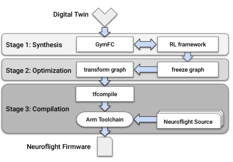
Figure 4$\cdot$2: Overview of the Neuroflight toolchain.

4.4.1 Synthesis

The synthesis stage takes as input a digital twin of an aircraft and synthesizes a NN attitude flight controller capable of achieving stable flight in the real world. Our toolchain can support any RL library that interfaces with OpenAI environment APIs and allows for the NN state to be saved as a Tensorflow graph. Currently our toolchain uses RL algorithms provided by OpenAI baselines [Dhariwal et al., 2017] which has been modified to save the NN state. In Tensorflow, the saved state of a NN is known as a checkpoint and consists of three files describing the structure and values in the graph. Once training has completed, the checkpoint is provides as input to Stage 2: Optimization.

4.4.2 Optimization

The optimization stage is an intermediate stage between training and compilation that prepares the NN graph to be run on hardware. The optimization stage (and compilation stage) require a number of Tensorflow tools which can all be found in the Tensorflow repository [ten, 2018]. The first step in the optimization stage is to freeze the graph. Freezing the graph accomplishes two tasks: (1) condenses the three checkpoint files into a single Protobuf file by replacing variables with their equivalent constant values (e.g., numerical weight values) and (2) extracts the subgraph containing the trained NN by trimming unused nodes and operations that were only used during training. Freezing is done with Tensorflow’s freeze_graph.py tool which takes as input the checkpoint and the output node of the graph so the tool can identify and extract the subgraph.

Unfortunately the Tensorflow input and output nodes are not documented by RL libraries (OpenAI baselines [Dhariwal et al., 2017], Stable baselines [Hill et al., 2018], TensorForce [Schaarschmidt et al., 2017]) and in most cases it is not trivial to identify them. We reverse engineered the graph produced by OpenAI Baselines (specifically the PPO1 implementation) using a combination of tools and cross referencing with the source code. A Tensorflow graph can be visually inspected using Tensorflow’s Tensorboard tool. OpenAI Baselines does not support Tensorboard thus we created a script to convert a checkpoint to a Probobuf file and then used Tensorflow’s import_pb_to_tensorboard.py tool to view the graph in Tensorboard. Additionally we used Tensorflow’s summarize_graph tool to summarize the inputs and outputs of the graph. Ultimately we identified the input node to be “pi/ob”, and the output to be “pi/pol/final/BiasAdd”.

Once the graph is frozen, it is optimized to run on hardware by running the Tensorflow transform_graph tool. Optimization provided by this tool allows graphs to execute faster and reduce its overall footprint by further removing unnecessary nodes. The optimized frozen ProtoBuf file is provided as input to Stage 3: Compilation.

4.4.3 Compilation

A significant challenge was developing a method to integrate a trained NN into Neuroflight to be able to run on the limited resources provided by a microcontroller. The most powerful of the microcontrollers supported by Betaflight and Neuroflight consists of 1MB of flash memory, 320KB of SRAM and an ARM Cortex-M7 processor with a clock speed of 216MHz [STM, 2018]. Recently there has been an increase in interest for running NNs on embedded devices but few solutions have been proposed and no standard solution exists. We found Tensorflow’s tool tfcompile to work best for our toolchain. tfcompile provides ahead-of-time (AOT) compilation of Tensorflow graphs into executable code primarily motivated as a method to execute graphs on mobile devices. Normally executing graphs requires the Tensorflow runtime which is far too heavy for a microcontroller. Compiling graphs using tfcompile does not use the Tensoflow runtime which results in a self contained executable and a reduced footprint.

Tensorflow uses the Bazel [baz, 2018] build system and expects you will be using the tfcompile Bazel macro in your project. Neuroflight on the other hand is using make with the GNU Arm Embedded Toolchain. Thus it was necessary for us to integrate tfcompile into the toolchain by calling the tfcompile binary directly. When invoked, an object file representing the compiled graph and an accompanying header file is produced. Examining the header file we identified three additional Tensorflow dependencies that must be included in Neuroflight (typically this is automatically included if using the Bazel build system): the AOT runtime (runtime.o), an interface to run the compiled functions (xla_compiled_cpu_function.o), and running options (executable_run_options.o) for a total of 24.86 KB. In Section 4.5 we will analyze the size of the generated object file for the specific neuro-flight controller.

To perform fast floating point calculations Neuroflight must be compiled with ARM’s hard-float application binary interface (ABI). Betaflight core, inherited by Neuroflight already defines the proper compilation flags in the Makefile however it is required that the entire firmware must be compiled with the same ABI meaning the Tensorflow graph must also be compiled with the same ABI. Yet tfcompile does not currently allow for setting arbitrary compilation flags which required us to modify the code. Under the hood, tfcompile uses the LLVM backend for code generation. We were able to enable hard floating points through the ABIType attribute in the llvm::TargetOptions class.

4.5 Evaluation

In this section we evaluate Neuroflight controlling a high performance custom FPV racing quadcopter named NF1, pictured in Fig. 4$\cdot$3(b). First and foremost, we show that it is capable of maintaining stable flight. Additionally, we demonstrate that the synthesized NN controller is also able to stabilize the aircraft even when executing advanced aerobatic maneuvers. Additional images of NF1 and its entire build log have been published to RotorBuilds [rot, 2018].

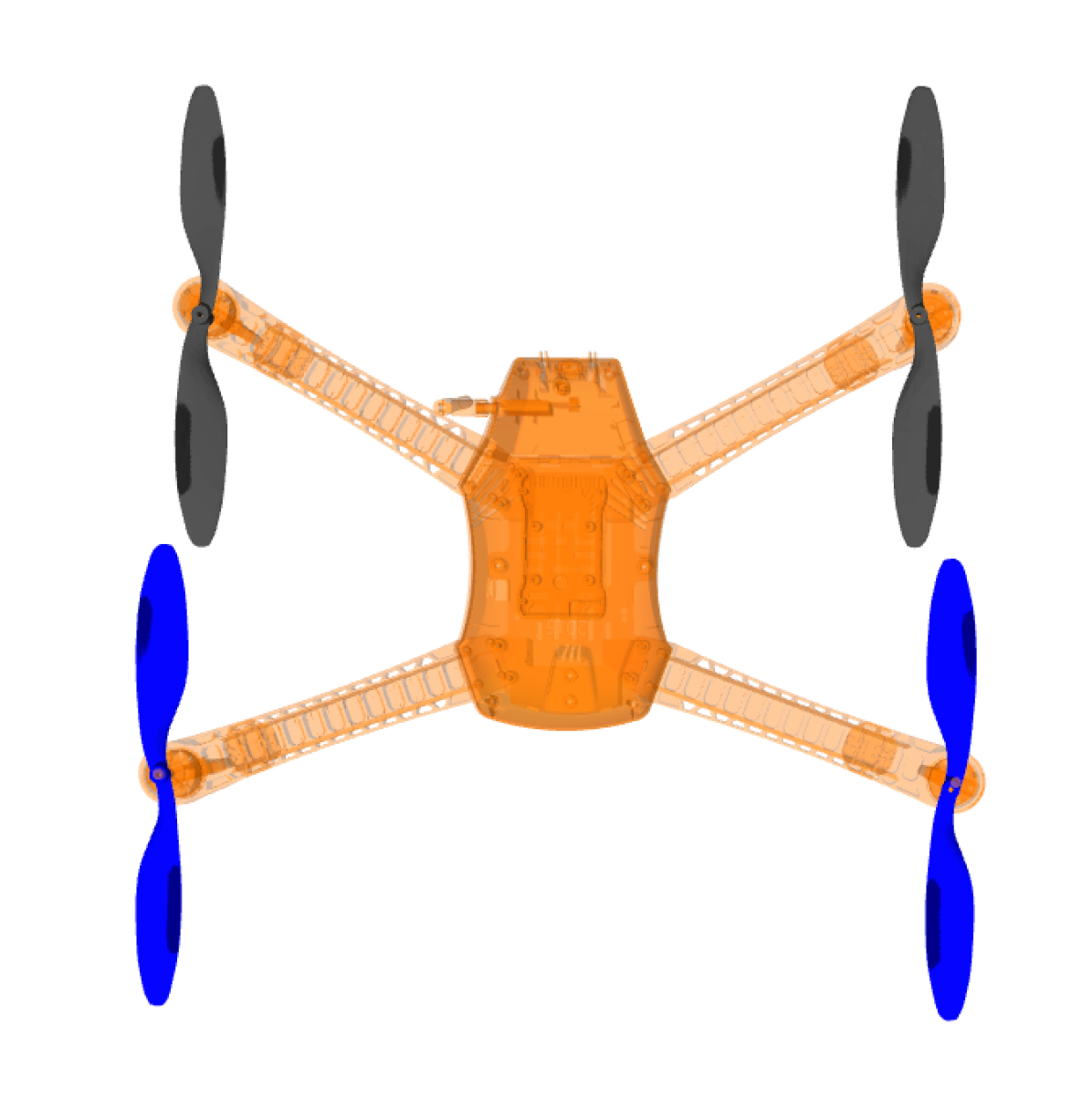
(a) Iris

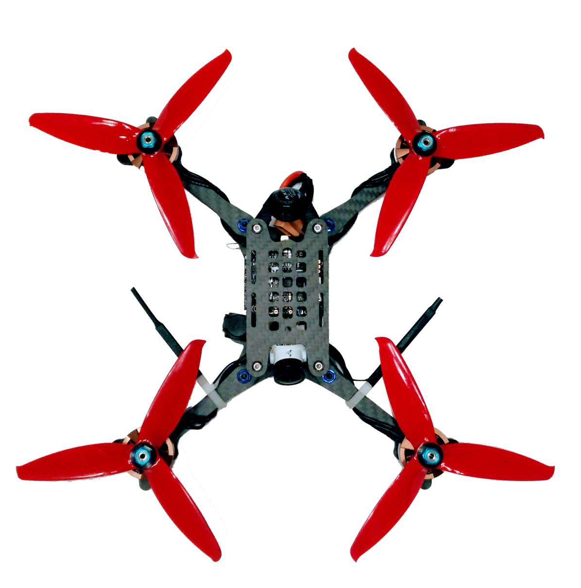
(b) NF1

Figure 4$\cdot$3: Iris simulated quadcopter compared to the NF1 real quadcopter.

4.5.1 Firmware Construction

We used the Iris quadcopter model included with the Gazebo simulator (which is also used by GymFCv1) with modifications to the motor model to more accurately reflect NF1 for our digital twin. The digital twin motor model used by Gazebo is quite simple. Each control signal is multiplied by a maximum rotor velocity constant to derive the target rotor velocity while each rotor is associated with a PID controller to achieve this target rotor velocity. We obtained an estimated maximum 33,422 RPMs for our propulsion system from Miniquad Test Bench [min, 2018] to update the maximum rotor velocity constant. We also modified the rotor PID controller (P=0.01, I=1.0) to achieve a similar throttle ramp.

NF1 is in stark contrast with the Iris quadcopter model used by GymFCv1 which is advertised for autonomous flight and imaging [iri, 2018]. We have provided a visual comparison in Fig. 4$\cdot$3 and a comparison between the aircraft specifications in Table 4.1. In this table, weight includes the battery, while the wheelbase is the motor to motor diagonal distance. Propeller specifications are in the format “LL:PPxB” where LL is the propeller length in inches, PP is the pitch in inches and B is the number of blades. Brushless motor sizes are in the format “WWxHH” where WW and HH is the stator width and height respectively. The motors $K_{v}$ value is the motor velocity constant and is defined as the inverse of the motors back-EMF constant which roughly indicates the RPMs per volt on an unloaded motor [lea, 2015]. Flight controllers are classified by the version of the embedded ARM Cortex-M processor prefixed by the letter ‘F’ (e.g., F4 flight controller uses an ARM Cortex-M4).

	Iris	NF1
Weight	1282g	432g
Wheelbase	550mm	212mm
Propeller	10:47x2	51:52x3
Motor	28x30 850$K_{v}$	22x04 2522$K_{v}$
Battery	3-cell 3.5Ah LiPo	4-cell 1.5Ah LiPo
Flight Controller	F4	F7

Table 4.1: Comparison between Iris and NF1 specifications.

Our NN architecture consists of 6 inputs, 4 outputs, 2 hidden layers with 32 nodes each using hyperbolic tangent activation functions resulting in a total of 1,344 tunable weights. The network outputs the mean of a Gaussian distribution with a variable standard deviation as defined by PPO for continuous domains [Schulman et al., 2017]. Training was performed with the OpenAI Baseline version 0.1.4 implementation of PPO1 due to its previous success in Chapter 3 which showed PPO to out perform DDPG [Lillicrap et al., 2015], and TRPO [Schulman et al., 2015] in regards to attitude control in simulation. A picture of the quadcopter during trained in GymFCv1.5 can be seen in Fig. 4$\cdot$4(a).

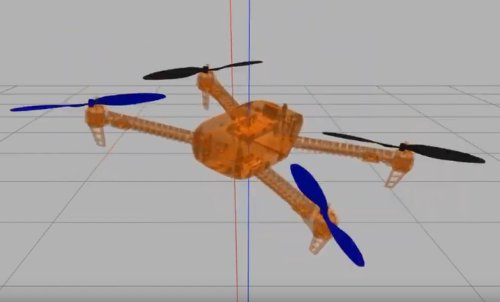
(a) Screenshot of the Iris quadcopter flying in simulation.

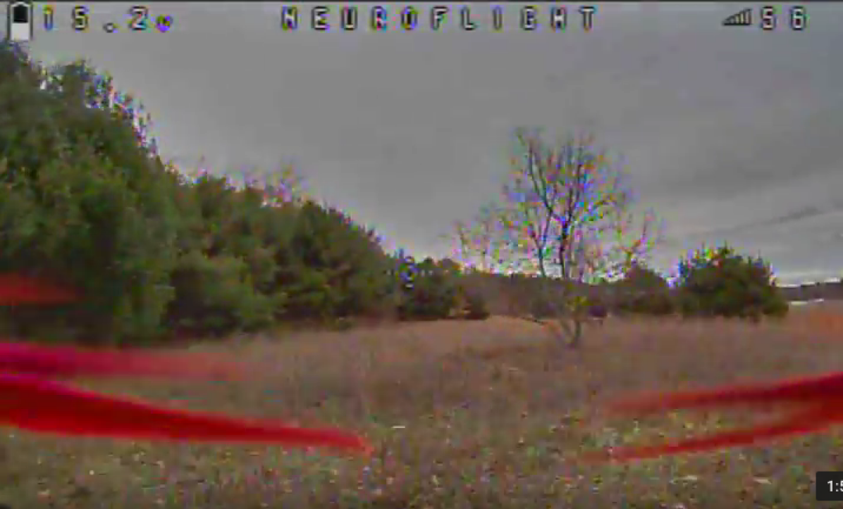
(b) Still frame of the FPV video footage acquired during a test flight.

Figure 4$\cdot$4: Flight in simulation (left) and in the real world (right).

The reward system hyperparameters used were $\alpha=300$, $\beta=0.5$, and $\Delta y_{max}=100^{2}$ and the PPO hyperparameters used are reported in Table 4.2. The reward hyperparameter $\Delta y_{max}$ is defined as the maximum delta in the output we are willing to accept, while $\alpha$ and $\beta$ were found through experimentation to find the desired balance between minimizing the output and minimizing the output oscillations. The discount and Generalized Advantage Estimate (GAE) parameters were taken from [Schulman et al., 2017] while the remaining parameters were found using random search. The agent was particularity sensitive to the selection of the horizon and minibatch size. To account for sensor noise in the real world we added noise to the angular velocity measurements which was sampled from a Gaussian distribution with $\mu=0$ and $\sigma=5$. The standard deviation was obtained by incrementing $\sigma$ until it began to impact the controllers ability to track the setpoint in simulation. We observed this to reduce motor oscillations in the real world.

A challenge we faced transferring the trained policy to hardware was that we were unable to get the quadcopter to idle. The control signals generated at at idle, $\Omega^{*}=[0,0,0]$, was producing a net force greater than the downward force of our aircraft. As a result, the quadcopter would not stay on the ground. A possible explanation to this behavior could be due to the differences between the simulated quadcopter and the real quadcopter. As a work around to make it easier for the agent to generate small control signals, we disabled gravity in the training environment. By doing so the agent does not have to fight the additional force of gravity while still being able to learn the relationship between the angular velocity and control outputs. In the real world, as long as a minimum throttle value is mixed in to the output of the NN during flight (e.g., either manually by the pilot or by configuring the firmware) such that the net force is greater or equal to zero, it will provide stable flight. Of course neglecting this force results in a less accurate representation of the real world. However our immediate goal is to show transferability. In future work we plan to investigate alternative environments to teach the quadcopter to idle without sacrificing real world dynamics. One possibility is to include a quaternion $q$ defining the quadcopters orientation, and the current throttle value as part of the aircraft state. Therefore the agent can be taught when $\textbf{T}=0$ and $q=[x=0,y=0,z=0,w=1]$ (i.e., no thrust and no rotation), to minimize the output small enough to idle.

Hyperparameter	Value
Horizon (T)	500
Adam stepsize	$1\times 10^{-4}\times\rho$
Num. epochs	5
Minibatch size	32
Discount ($\gamma$)	0.99
GAE parameter ($\lambda$)	0.95

Table 4.2: PPO hyperparameters where $\rho$ is linearly annealed over the course of training from 1 to 0.

Each training task/episode ran for 30 seconds in simulation. The simulator is configured to take simulation steps every 1ms which results in a total of 30,000 simulation steps per episode. Training ran for a total of 10 million time steps (333 episodes) on a desktop computer running Ubuntu 16.04 with an eight-core i7-7700 CPU and an NVIDIA GeForce GT 730 graphics card which took approximately 11 hours. However training converged much earlier at around 1 million time steps (33 episodes) in just over an hour (Fig. 4$\cdot$5). We trained a total of three NNs which each used a different random seed for the RL training algorithm and selected the NN that received the highest cumulative reward to use in Neuroflight. Fig. 4$\cdot$5 shows a plot of the cumulative rewards of each training episode for each of the NNs. The plot illustrates how drastic training episodes can vary simply due to the use of a different seed.

The optimization stage reduced the frozen Tensorflow graph of the best performing NN by 16% to a size of 12KB. The graph was compiled with Tensorflow version 1.8.0-rc1 and the firmware was compiled for the MATEKF722 target corresponding to the manufacturer and model of our flight controller MATEKSYS Flight Controller F722-STD. Our flight controller uses the STM32F722RET6 microcontroller with 512KB flash memory, and 256KB of SRAM.

We inspected the .text, .data and .bss section headers of the firmware’s ELF file to derive a lower bound of the memory utilization. These sections totalled 380KB, resulting in at least 74% utilization of the flash memory. Graph optimization accounted for a reduction of 280B, all of which was reduced from the .text section. Although in terms of memory utilization the optimization stage was not necessary, this however will be more important for larger networks in the future. Comparing this to the parent project, Betaflight’s sections totalled 375KB.

Using Tensorflow’s benchmarking tool we performed one million evaluations of the graph with and without optimization and found the optimization processes to reduce execution time on average by $1.1\mu s$.

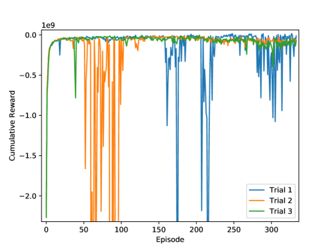
Figure 4$\cdot$5: Cumulative rewards for each training episode.

4.5.2 Simulation Evaluation

In this section we validate the best performing NN in simulation using the GymFCv1.5 environment. We execute the trained NN for five episodes in the environment for a total of 2.5 minutes simulation time. A zoomed in portion of one of the episodes is illustrated in Figure 4$\cdot$6. This figure also displays the control signals generated by the NN which is the value sent to the ESC. Note this is a different representation than that used in Chapter 3 which used PWM control signals. This is because the output must match that of the target flight control firmware for seamless transferability. If we compare the control output to that of the trained agent in Chapter 3, for example in Figure 3$\cdot$8, we can observe the impact this reward system has on reducing control signal values and oscillations.

From these validation episodes we computed the average performance metrics in Table 4.3. The controller does a decent job tracking the trajectory however it does suffer from overshooting the target particularly for the yaw axis which results in an increased error.

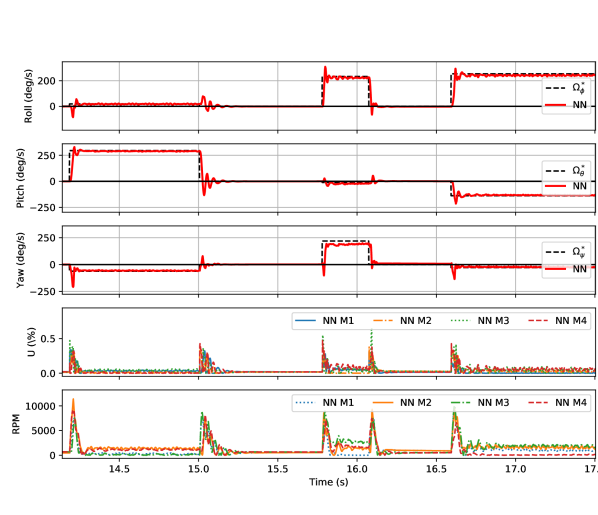
Figure 4$\cdot$6: Simulation validation of trained NN in GymFCv1.5 training environment. Actual aircraft angular velocity is represented by the red line, while the desired angular velocity is the dashed black line. Control signal and motor velocity is also shown.

	NN Controller (PPO)
Metric	Roll ($\phi$)	Pitch($\theta$)	Yaw ($\psi$)	Average
MAE	12	10	21	14
MSE	989	902	3,033	1,641
IAE	12,557	10,491	21,711	14,919
ISE	989,863	902,243	3,033,486	1,641,864
ITAE	180,688	152,279	324,266	219,078
ITSE	12,944,056	12,507,006	40,928,038	22,126,367

Table 4.3: Performance metric for NN training validation. Metric is reported for each individual axis, along with the average. Lower values are better.

4.5.3 Timing Analysis

Running a flight control task with a fast control rate allows for the use of a high speed ESC protocol, reducing write latency to the motors and thus resulting in higher precision flight. Therefore it is critical to analyze the execution time of the neuro-flight control task so the optimal control rate of the task can be determined. Once this is identified it can be used to select which ESC protocol will provide the best performance. We collect timing data for Neuroflight and compare this to its parent project Betaflight. Times are taken for when the quadcopter is disarmed and also armed under load for the control algorithm (i.e., evaluation of the NN and PID equation) and also the entire flight control task which in addition to the control algorithm includes reading the gryo, reading the RC commands and writing to the motors.

		WCET ($\mu s$)	BCET ($\mu s$)	Var. Window (%)
Disarmed	Neuroflight	204	194	4.9
	Betaflight	14	9	35.7
Armed	Neuroflight	210	195	7.1
	Betaflight	15	9	40.0

Table 4.4: Control algorithm timing analysis.

We instrumented the firmware to calculate the timing measurement and wrote the results to an unused serial port on the flight control board. Connecting to the serial port on the flight control board via an FTDI adapter we are able to log the data on an external PC running minicom. We recorded 5,000 measurements and report the worst-case execution time (WCET), best-case execution time (BCET) and the variability window in Table 4.4 for the control algorithm and Table 4.5 for the control task. The variability window is calculated as the difference between the WCET and BCET, normalized by the WCET, i.e., $(\text{WCET}-\text{BCET})/\text{WCET}$. This provides indication of how predicable is the execution of the flight control logic, as it embeds information about the relative fluctuation of execution times. Two remarks are important with respect to the results in Table 4.4. First, the NN compared to PID is about 14x slower (armed case), although the predictability of the controller increases. It is important to remember that, while executing the PID is much simpler than evaluating an NN, our approach allows removing additional logic that is required by a PID, such as motor mixing. Thus, a more meaningful comparison needs to be performed by looking at the overall WCET and predictability of the whole flight control task, which we carry out in Table 4.5. Second, because the NN evaluation always involve the same exact steps, an improvement in terms of predictability can be observed under Neuroflight.

		WCET $(\mu s)$	BCET $(\mu s)$	Var. Window (%)
Disarmed	Neuroflight	244	229	6.1
	Betaflight	58	45	22.4
Armed	Neuroflight	423	263	37.8
	Betaflight	238	78	67.2

Table 4.5: Flight control task timing analysis.

The timing analysis reported in Table 4.5 reveals that the neuro-flight control task has a WCET of 423 $\mu s$ which would allow for a max execution rate of 2.4kHz. However in Neuroflight (and in Betaflight), the flight control task frequency must be a division of the gyro update frequency, thus with 4kHz gyro update and a denominator of 2, the neuro-flight control task can be configured to execute at 2kHz. To put this into perspective this is 8 times faster than the popular PX4 firmware [Meier et al., 2015].

Furthermore this control rate is 40 times faster than the traditional PWM ESC protocol used by commercial quadcopters (50Hz [Abdulrahim et al., 2019]) thereby allowing us to configure Neuroflight to use the ESC protocol DShot600 which has a max frequency of 37.5kHz  [Liang, 2018].

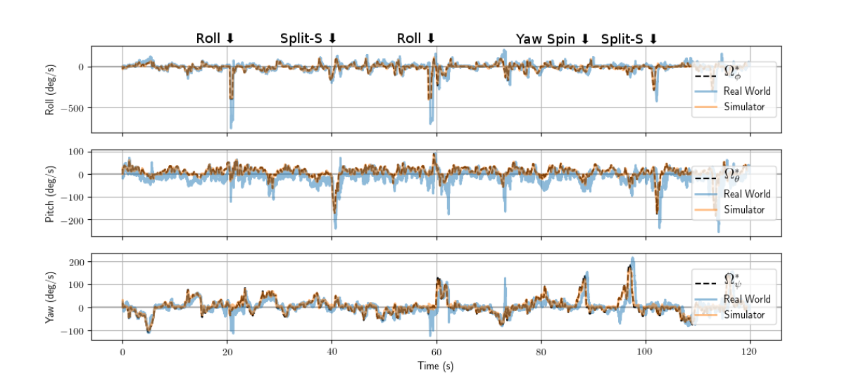
Figure 4$\cdot$7: Flight test log demonstrating Neuroflight tracking a desired angular velocity in the real world compared to in simulation. Maneuvers during this flight are annotated.

Given the simplicity of the PID algorithm it came as no surprise that the Betaflight flight control task is faster, yet this is only by a factor of 1.78 when armed. As we can see comparing Table 4.4 to Table 4.5 the additional subprocesses tasks are the bottleneck of the Betaflight flight control ask. However referring to the variability window, the Neuroflight control algorithm and control task are far more stable than Betaflight. The Betaflight flight control task exhibits little predictability when armed.

Recent research has shown there is no measurable improvements for control task loop rates that are faster than 4kHz [Abdulrahim et al., 2019]. Our timing analysis has shown that Neuroflight is close of this goal. To reach this goal there are three approaches we can take: (1) Support future microcontrollers with faster processor speeds, (2) experiment with different NN architectures to reduce the number of arithmetic operations and thus reduce the computational time to execute the NN, and (3) optimize the flight control sub tasks to reduce the flight control task’s WCET and variability window. In future work we immediately plan to explore (2) and (3), results obtained in these directions would not depend on the specific hardware used in the final assembly.

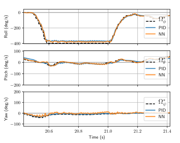
(a) Roll

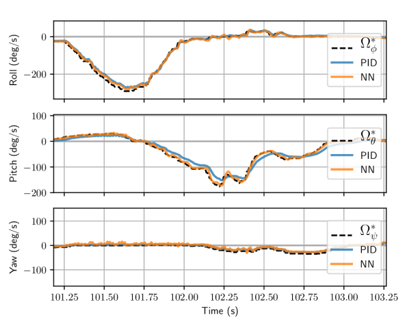
(b) Split-S

Figure 4$\cdot$8: Performance comparison of the NN controller versus a PID controller tracking a desired angular velocity in simulation to execute the Split-S and roll aerobatic maneuvers.

4.5.4 Power Analysis

The flight controller affects power consumption directly and indirectly. The direct power draw is a result of the execution of the control algorithm/task, while the indirect power draw is due to the generated control signals which determines the amount of power the ESC will draw.

As a first attempt to understand and compare the power consumption of a NN based controller to a standard PID controller, we performed a static power analysis. For NF1 running Neuroflight, we connected a multimeter inline with the battery power supply to measure the current draw and report the measurements for both when the quadcopter is disarmed (direct power consumption) and armed idling (indirect power consumption), similarly done to our timing analysis. We then take the same measurements for the NF1 running Betaflight (PID control). Results reported in Table 4.6 show there is no change using the NN based controller in regards to direct power draw of the control algorithm. This result was expected as the flight control firmware does not execute sleep instructions. However for the indirect power draw, there is a measurable 70mA (approximately 11%) increase in current draw for the NN controller. It is important to remember this particular NN controller has been trained to optimize its ability to track a desired angular velocity. Thus the increase in current draw does not come as a surprise as the control signals will be required to switch quickly to maintain the set point which results in increased current draw.

An advantage a NN controller has over a traditional PID controller is that it has the ability to optimize its performance based on a number of conditions and characteristics, such as power consumption. In the future we will investigate alternative optimization goals for the controller and instrument NF1 with sensors to record power consumption in flight to perform a thorough power analysis.

		Voltage (V)	Current (A)	Power (W)
Disarmed	Neuroflight	16.78	0.37	6.21
	Betaflight	16.78	0.37	6.21
Armed	Neuroflight	16.78	0.67	11.24
	Betaflight	16.78	0.6	10.07

Table 4.6: Power analysis of Neuroflight compared to Betaflight.

4.5.5 Flight Evaluation

To test the performance of Neuroflight we had an experienced drone racing pilot conduct five test flights for us. The FPV videos of the test flights can be viewed at [Koch, 2018c]. A still image extracted from the FPV video feed shows the view point of the pilot of one of the test flights can be seen in Fig. 4$\cdot$4(b). In FPV flying the aircraft has a camera which transmits the analog video feed back to the pilot who is wearing goggles with a monitor connected to a video receiver. This allows the pilot to control the aircraft from the perspective of the aircraft.

Neuroflight supports real-time logging during flight allowing us to collect gyro and RC command data to analyze how well the neuro-flight controller is able to track the desired angular velocity. We asked the pilot to fly a mix of basic maneuvers such as loops and figure eights and advanced maneuvers such as rolls, flips, dives and the Split-S. To execute a Split-S the pilot inverts the quadcopter and descends in a half loop dive, exiting the loop so they are flying in the opposite horizontal direction. Once we collected the flight logs we played the desired angular rates back to the NN in the GymFCv1.5 environment to evaluate the performance in simulation. This allows the performance gap between the two environments to be measured and identify the reality gap. Comparison between the simulated and real world performance for one of the test flights is illustrated in Fig. 4$\cdot$7 while specific maneuvers that occur during this test flight are annotated. We computed various error metrics for the flights including the Mean Absolute Error (MAE), and Mean Squared Error (MSE), as well as the discrete form of the Integral Absolute Error (IAE), Integral Squared Error (ISE), Integral Time-weighted Absolute Error (ITAE), and Integral Time-weighted Squared Error (ITSE). These values are reported in Table 4.7 are an average for the real flights and in Table 4.8 for the simulated flight .

	NN Controller (PPO)
Metric	Roll ($\phi$)	Pitch($\theta$)	Yaw ($\psi$)	Average
MAE	15	21	13	16
MSE	1,720	1,860	686	1,422
IAE	15,176	21,160	13,478	16,605
ISE	1,711,764	1,851,450	682,914	1,415,376
ITAE	705,614	1,001,476	638,513	781,868
ITSE	98,725,074	90,438,678	37,397,559	75,520,437

Table 4.7: Error metrics of the NN controller from 5 flight in the real world. Metrics are reported for each individual axis, along with the average. Lower values are better.

	NN Controller (PPO)
Metric	Roll ($\phi$)	Pitch($\theta$)	Yaw ($\psi$)	Average
MAE	3	2	4	3
MSE	23	6	27	19
IAE	2,888	1,523	4,072	2,827
ISE	23,227	5,589	27,203	18,673
ITAE	179,945	93,339	261,947	178,410
ITSE	1,499,076	369,577	1,893,954	1,254,202

Table 4.8: Error metrics for simulation playback using NN controller. Metric is reported for each individual axis, along with the average. Lower values are better.

	PID
Metric	Roll ($\phi$)	Pitch($\theta$)	Yaw ($\psi$)	Average
MAE	4	5	3	4
MSE	35	46	21	34
IAE	3,905	5,258	3,423	4,195
ISE	34,811	45,590	20,549	33,650
ITAE	236,408	320,205	217,343	257,985
ITSE	2,100,576	2,927,031	1,419,391	2,148,999

Table 4.9: Error metrics for simulation playback using PID controller. Metric is reported for each individual axis, along with the average. Lower values are better.

As we can see there is a considerable increase in error (16 degrees per second on average) transferring from simulation from reality, however this was expected because the digital twin does not perfectly model the real system. There is a large increase in error for the integral measurements. A partial explanation for this is if we refer to Fig. 4$\cdot$7 (particularly the pitch axis) we can see the controller is consistently off by about 10 degrees which will continually add error to these measurements. Additionally the difference in squared errors is quite significant which will emphasize larger errors that occur.

The increased error on the pitch axis appears to be due to the differences in frame shape between the digital twin and real quadcopter, which are both asymmetrical but in relation to a different axis. This discrepancy may have resulted in pitch control lagging in the real world as more torque and power is required to pitch in our real quadcopter.

We also compared the average absolute difference in the control signals ($\overline{|\Delta u|}$) between the two worlds. In simulation we found this to be $0.007\pm 1e-4$, while in the real world there was a minor increase to $0.01\pm 5.5e-5$ but we found this did not result in any harm to the motors such as a noticeable increase in output oscillations or heat being generated.

A more accurate digital twin model can boost accuracy. Furthermore, during this particular flight wind gusts exceeded 30mph, while in the simulation world there are no external disturbances acting upon the aircraft. In the future we plan to deploy an array of sensors to measure wind speed so we can correlate wind gusts with excessive error. Nonetheless, as shown in the video, stable flight can be maintained demonstrating the transferability of a NN trained with our approach.

PID vs NN Control. Next we performed an experiment to compare the performance of the NN controller used in Neuroflight to a PID controller in simulation using the GymFCv1.5 environment. Although other control algorithms may exist in literature that out perform PID, of the open source flight controllers available for benchmarking, every single one uses PID [Ebeid et al., 2018]. A major contribution of this work is providing the research community an additional flight control algorithm for benchmarking.

The PID controller was tuned in simulation using the classical Ziegler-Nichols method [Ziegler and Nichols, 1942] and then manually adjusted to reduce overshoot to obtained the following gains for each axis of rotation: $K_{\phi}=[0.032029,0,0.000396]$, $K_{\theta}=[0.032029,0,0.000396]$, $K_{\psi}=[0.032029,0,0]$, where $K_{\text{axis}}=[K_{p},K_{i},K_{d}]$ for each proportional, integrative, and derivative gains, respectively. It took approximately a half hour to manually tune the 9 gains with the bottleneck being the time to execute the simulator in order to obtain the parameters to calculate Ziegler-Nichols. In comparison to training a NN via PPO, there is not a considerable overhead difference given this is an offline task. In fact the tuning rate by PPO is significantly faster by a factor of 75.

The RC commands from the real test flight where then replayed back to the simulator similar to the previous experiment, however this time using the tuned PID controller. A zoomed in comparison of the NN and PID controller tracking the desired angular velocity for two aerobatic maneuvers is shown in Fig. 4$\cdot$8. Although the performance is quite close, we can most visibly the NN controller tracking the pitch axis during a Split-S maneuver more accurately.

We also computed the same control measurements for the PID controller and reported them in Table 4.9. Results show, on average, the NN controller to outperform the PID controller for every one of our metrics.

It is important to note PID tuning is a challenging task and the PID controller’s accuracy and ability to control the quadcopter is only as good as the tune. The NN controller on the other hand did not require any manually tuning, instead through RL and interacting with the aircraft over time it is able to teach itself attitude control. As we continue to the reduce the gap between simulation and the real world, the performance of the NN controller will continue to improve in the real world.

4.6 Future Work and Conclusion

In this chapter we introduced Neuroflight, the first open-source neuro-flight control firmware for multicopters and fixed wing aircraft and its accompanying toolchain. There are four main directions we plan to pursue in future work.

1. Digital twin development. In this work we synthesized our NN using an existing quadcopter model that did not match NF1. Although stable flight was achieved demonstrating the NNs robustness, comparison between the simulated flight verse the actual flight is evidence inaccuracies in the digital twin has a negative affect in flight control accuracy. In future work we will develop an accurate digital twin of NF1 and investigate how the fidelity of a digital twin affects flight performance in an effort to reduce costs during development.

2. Adaptive and predictive control. With a stable platform in place we can now begin to harness the NN’s true potential. We will enhance the training environment to teach adaptive control to account for excessive sensor noise, voltage sag, change in flight dynamics due to high throttle input, payload changes, external disturbances such as wind, and propulsion system failure.

3. Continuous learning. Our current approach trains NNs exclusively using offline learning. However, in order to reduce the performance gap between the simulated and real world, we expect that a hybrid architecture involving online incremental learning will be necessary. Online learning will allow the aircraft to adapt, in real-time, and to compensate for any modelling errors that existed during synthesis of the NN during offline (initial) training. Given the payload restrictions of micro-UAVs and weight associated with hardware necessary for online learning we will investigate methods to off-load the computational burden of incremental learning to the cloud.

4. NN architecture development. Several performance benefits can be realized from an optimal network architecture for flight control including improved accuracy (Section 4.5.5) and faster execution (Section 4.5.3). In future work we plan to explore recurrent architectures utilizing long short-term memory (LSTM) to improve accuracy. Additionally we will investigate alternative distributions such as the beta function which is naturally bounded [Chou et al., 2017]. Furthermore we will explore the use of the rectified linear unit (ReLU) activation functions to increase execution time which is more computationally efficient than the hyperbolic tangent function.

The economic costs associated with developing neuro-flight control will foreshadow its future, determining whether its use will remain confined to special purpose applications, or if it will be adopted in mainstream flight control architectures. Nonetheless, we strongly believe that Neuroflight is a major milestone in neuro-flight control and will provide the required foundations for next generation flight control firmwares.

Chapter 5 Aircraft Modelling for In Silico Neuro-flight Controller Synthesis

Tuning controllers in silico (i.e., in simulation) has numerous advantages over tuning in the real world. It is cost effective, runs faster than real time, allows for rapid prototyping and testing, and it is easily automated. Additionally, the controller can be exposed to environments and conditions that would otherwise be difficult and expensive to do in the real world (e.g., part failure, extreme weather, etc). Unfortunately it can be very challenging to obtain the same level of performance from the controller when transferred to hardware operating in the real world. This is primarily due to the simulator failing to capture all of the dynamics in the controller’s real world operating environment. To provide seamless transferability to hardware, the ultimate goal would be to eliminate the reality gap. But the world is a highly complex place with many unknowns. Modelling the known dynamics can require an extraordinary level of computation.

Several methods have been proposed to aid in transferring the NN trained in simulation to the real world such as sampling data from the real world environment, and integrating it into the simulation environment [Jakobi et al., 1995]. Additionally, injecting noise and domain randomizing have also been shown to improve performance in the real world [Tobin et al., 2017, Andrychowicz et al., 2018, Molchanov et al., 2019]. The idea behind these techniques is to train the NN on copious variations of the environment such that the actual real world just appears as another variation to the NN. This essentially blurs the reality gap for the controller.

To further improve performance, an ideal control system would, in addition, provide online tuning to account for unknown dynamics found in the real world. These tuning strategies form building blocks for hierarchical tuning (learning) frameworks. However before online tuning can be utilized, the controller must first be tuned in silico well enough to operate in the real world.

In Chapter 4 our quadcopter achieved stable flight in the real world with a NN-based controller trained by GymFCv1.5 via RL. However there was a significant, but expected, gap between the performance observed in simulation compared to the real world due to the inaccuracies in the aircraft model used during training. In this chapter we propose our methodology for creating a digital twin for a multicopter and use this methodology to create a digital twin of our aircraft, NF1. In summary this chapter makes the following contributions:

• GymFCv2, a universal flight control tuning framework. As a prerequisite to creating the digital twin, it was first necessary to revise GymFCv1.5 to easily support any aircraft. This update provides a framework for tuning any control algorithm, not just NN-based flight controllers. In addition to using the framework for training neuro-flight controller policies, we also demonstrate its modular design implementing a dynamometer simulation for validating motor performance, and a PID tuning platform.

• A methodology for creating multicopter digital twins. We outline, from the ground up, how to create a digital twin of a multicopter. This consists of creating the rigid bodies and modelling motor dynamics. To measure performance characteristics of our propulsion system we develop a dynamometer for collecting rotor velocity, thrust and torque measurements.

• Propulsion system modelling enhancements. Building upon the PX4 SITL motor models [px4, 2019], this work introduces enhancements to modelling motor response and throttle curves. These models have been ported to the GymFCv2 framework and have been made open source available from [Koch, 2019a].

• A simulation stability analysis. Multicopters are extremely agile, due to having full rotational range of motion, independent of translational motion. Aggressive angular velocity maneuvers are subjected to high centripetal forces, in simulation, and also in the real world. However in simulation, significant forces can introduce simulation instabilities. In this work we introduce a tool for measuring model stability in simulation and compare these results using two different physics engines used by the Gazebo simulator.

• Implementation of GymFCv2 for synthesizing neuro-flight controllers trained via RL. We propose our user modules consisting of a new environment and reward function to further reduce errors and aid in transferring the trained policy to the real world.

• Evaluation of a neuro-flight controller synthesized with its digital twin. We first evaluate the neuro-flight controller in simulation and find it to exceed the performance of a PID controller, in regards to minimizing error, and also having a larger flight envelope. Next, we transfer the trained policy to hardware and perform a number of flight tests. Although our flight logs show control signals oscillations are high, they do not have any impact on the stability of the aircraft. In fact, in regards to tracking error, our analysis finds training on the digital twin greatly reduces error, resulting in a smoother more accurate controller than previously obtained.

The remainder of this chapter is organized as follows. In Section 5.1 we introduce GymFCv2 as a means to standardize flight control tuning in silico. Next, in Section 5.2, we propose our methodology for developing multicopter digital twins and walk through the processes of creating a digital twin for our aircraft NF1. In Section 5.3 we verify the stability of our digital twin in simulation before it is used for training. Next, we describe the changes we made to the training environment in Section 5.4 and then we evaluate the performance of the synthesized neuro-controller in Section 5.5. In Section 5.6 we review other flight simulators, aircraft models and data sources. Finally, in Section 5.7, we conclude with our final remarks and future work.

5.1 GymFCv2

In this section we introduce GymFCv2, a powerful tool for flight control development. The new version has a redesigned architecture to address limitations in the previous versions. An illustration of its typically usage is depicted in Fig. 5$\cdot$1.

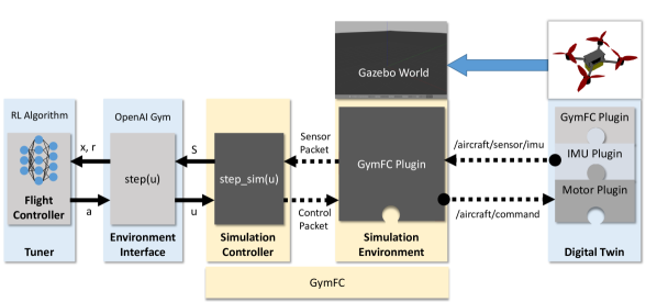
Figure 5$\cdot$1: Instance of GymFCv2 architecture for synthesizing RL-based flight controller.

The main drawbacks with the previous versions of GymFC is that it is tightly coupled to the aircraft model and was specifically developed as an RL environment. The new architecture of GymFCv2 is aircraft agnostic ( meaning it does not care what type of aircraft is being controlling) and is a generic tool for flight controller development (that is, it is not strictly for NN-based flight controllers). To synthesize optimal flight controllers, each controller must be trained for its unique aircraft digital twin. Thus the primary motivation for the new architecture was to provide an easy way to use any aircraft model.

To support a more generic framework, GymFCv1 was reduced to only the core implementation for providing the training environment and interfaces with the simulation environment and the aircraft. The remaining functionality has been moved to user provided modules. This increases flexibility allowing the client to provide their own controller environments and aircraft models. For example, this allows a user to test and develop any type of flight controller, not only for neuro-based controllers but also more traditional controllers such as PID. Additionally, for those developing neuro-based controllers, this allows the user to develop, maintain and version control their training interfaces independent of GymFC. Furthermore, reward engineering for RL-based training is a challenging problem dependent on many factors such as aircraft type and performance optimization goals. During development it will be common for users to be experimenting with different implementation which is easier to do within the new architecture.

In the remainder of this section we will first discuss the details of the GymFCv2 architecture and then the user provided modules.

5.1.1 Architecture

GymFCv2 consists of two modules, a simulation controller providing a client interface for interacting with the simulator and the simulator environment which provides the tuning environment and an aircraft interface.

Simulation Controller

The simulation controller is the client facing module in the form of a Python library. Its purpose is to provide an interface for the user to configure and control the tuning environment.

Configuration. GymFCv2 is initialized with an aircraft configuration file. The aircraft configuration file is in the SDF file format [sdf, 2019] which is an XML file with a schema specific for describing robots and their environments made popular by Gazebo. The configuration file describes the aircraft model for use by the Gazebo simulator such as the locations to the 3D mesh files, geometric properties, and also the definitions of the plugins to be loaded for modelling dynamics. In an SDF file, the plugin element contains a filename attribute that points to the name of a shared library to be loaded at run time.

To simply user configuration, without requiring multiple configuration files, information specifically needed by the GymFCv2 simulation environment is also embedded in the aircraft configuration. However due to constraints in the SDF schema, arbitrary XML elements are not allowed in the file. Fortunately, the SDF plugin element does allow for arbitrary elements to be defined. Thus as a workaround, the user must define our dummy plugin libAircraftConfigPlugin.so that contains the information needed by the GymFCv2 simulation environment plugin. This plugin does not provide any dynamic capabilities, it is merely a method to provide GymFCv2 configuration information.

This plugin defines the number of actuators the aircraft uses for control as well as the sensors that are supported by the aircraft. Knowledge of the supported sensors is strictly for optimization purposes which will be discussed later in this section.

For attitude controllers, the configuration must also specify the aircraft’s center of thrust which the simulator environment will use to fix the aircraft to in the simulation world. An example of this plugin for our quadcopter, NF1, is displayed in Listing 1. Although our aircraft supports additional sensors, for training and tuning purposes we only require angular velocity values.

⬇

<plugin name="cfg" filename="libAircraftConfigPlugin.so">

<motorCount>4</motorCount>

<centerOfThrust>

<link>battery</link>

<offset>0 0 0.058</offset>

</centerOfThrust>

<sensors>

<sensor type="imu">

<enable_angular_velocity>true</enable_angular_velocity>

</sensor>

</sensors>

</plugin>

Listing 1: NF1 configuration for GymFCv2

Simulation Control. The client can control the simulator in two ways (1) stepping the simulator through the step_sim function and (2) resetting the simulator and aircraft state by the reset function. The step_sim function takes as input an array of control signals $u$ for each aircraft actuator and performs a single simulation step, returning a flattened array of the aircraft sensor values in order as defined in the aircraft configuration file. The controller also exposes class attributes for the sensor values to be accessed directly.

The simulation controller communicates with the simulation environment through a UDP network channel which encodes the control signal and sensor messages in Google Protobuf messages.

Simulation Environment

The simulation environment (specifically the Gazebo GymFCv2 plugin) provides the majority of the heavy lifting and is constructed specifically for the task of tuning flight controllers. The environment supports attitude control tuning as in the initial version, as well as environments for motor modelling and navigation tasks. The new architecture also allows users to provide their own simulation worlds for more complex training such as obstacle avoidance. The simulation environment can be thought of as a Gazebo simulation wrapper with custom APIs for interacting with an aircraft in simulation.

Upon launch, the environment reads the location of aircraft configuration file from an environment variable set by the simulation controller. The environment then dynamically loads the aircraft model into the simulator and is ready to start accepting motor control messages from the controller. These motor messages also doubles as the simulation clock, every call to step_sim sends a motor message triggering a simulation step.

A challenge encountered dynamically loading the aircraft model was developing a communication channel to send and receive messages from the aircraft while still remaining decoupled from GymFCv2. We solved this problem by developing a topic based publish-subscribe messaging API which is summarized in Table 5.1. This API provides messages for sending the motor control signals, as well as reading sensors. Additionally, values such as motor torque and force exist which can be beneficial for motor model validation and reward engineering. In the future we plan to support additional sensors to aid in navigation tasks such video, sonar, and LIDAR.

During initialization, the GymFCv2 simulation plugin initializes a publisher for the /aircraft/command topic, and will also subscribe to every sensor topic of the sensors enabled in the aircraft configuration file. The enabled senors are required by the aircraft configuration to allow the GymFCv2 plugin to know it has received all of the sensor messages before returning the state back to the controller. At a high level, the following events complete a single simulation step,

1. Upon receiving a motor control message from the simulation controller, publish topic /aircraft/command with an array of the control signals, where the array index corresponds to the motor/actuator identifier.

2. Increment the simulation one time step. This triggers any digital twin plugin to execute.

3. Wait to receive sensor messages from the enabled /aircraft/sensor topics.

4. Pack received sensor values and simulation state into single message and send back to the simulation controller.

This decoupled communication channel provides the aircraft model designer the freedom to implement a variety of different aircraft architectures, without requiring GymFCv2 to know these details. For example, a designer may choose to model a single virtual ESC as one plugin which will subscribe to the /aircraft/command topic (i.e., one to one) while another option would be have a separate ESC/motor plugin instances for each motor who will each subscribe to the command topic and extract their value at the corresponding array index (i.e., one to many).

Although the publish-subscribe API provides a modular, flexible channel, it does increase complexity due to its asynchronous behavior. Messages are received out of order thus the GymFCv2 plugin uses a rendezvous point which blocks the state from being sent to the simulation controller until all sensor value are received. This enforces the required sequential time steps between the simulation controller and its environment.

Topic	Direction	Values
/aircraft/command	$\rightarrow$	Control Signals
/aircraft/sensor/imu	$\leftarrow$	Angular Velocity
		Linear Acceleration
		Orientation
/aircraft/sensor/esc/$<$id$>$	$\leftarrow$	Angular Velocity
		Temperature
		Voltage
		Current
		Force
		Torque
/aircraft/sensor/current	$\leftarrow$	Current
/aircraft/sensor/voltage	$\leftarrow$	Voltage
/aircraft/sensor/gps	$\leftarrow$	Longitude and Latitude

Table 5.1: Digital twin API. This table summarizes the topics and their corresponding message values. Direction specifies who is the publisher where $\rightarrow$ is a message published by the flight controller plugin and $\leftarrow$ is a message published by a sensor.

5.1.2 User Provided Modules

A typical instance of GymFCv2 is composed of four additional user provided modules: a flight control algorithm, a flight control algorithm tuner, an environment interface, and a digital twin. The modules provide researchers and developers an easy way to share. A number of off-the-self solutions exist for the first two modules, however custom implementations are typically required for developing the environment interface and the aircraft model. This section will describe each in detail.

Flight controller algorithm. The flight control algorithm performs some evaluation to derive the motor control signals. The algorithm can generically be represented as the function $u(t)=f(S(t),w)$ which takes as input the current state representation of the aircraft $S(t)$ and a set of tunable parameters $w$ and outputs an array of control signals $u(t)$ for each aircraft actuator. For example, this can be a NN-based controller with adjustable network weights $w=W$, or a PID controller with tunable gains $w=\{K_{P},K_{I},K_{D}\}$ for each roll, pitch and yaw axis. Our goal is to find $w$.

Flight controller algorithm tuner. The tuner interacts with the flight control algorithm and the environment interface to find an optimized $w$ depending on some performance goals (e.g., minimizing error, increasing flight time, etc). For NNs trained using RL, a number of off-the-self solutions exist such as OpenAI Baselines [Dhariwal et al., 2017], Tensorforce [Schaarschmidt et al., 2017], and others. These RL frameworks also provide the NN implementation.

Environment interface. The environment interface is intended to be a light weight shim that either inherits or creates an instance of the GymFCv2 simulation controller and performs any additional implementation required for interfacing with the control algorithm, and to support tuning.

It is common for the input and output of the control algorithm to differ from the aircraft state, and the actuator control signal respectively. For example, a NN controller with an output layer consisting of hyperbolic tangent activation functions (i.e., in the range $[-1,1])$ may be synthesized for a flight control firmware requiring each control signals to be in the range $u\in[0,1]$. Furthermore, for PID control (and also our NN), the input is a function of the error. The error must be computed from the angular velocity of the aircraft state. This module must provide a transformation function to provide these required mappings. The transformation function should implement the same API found in the target flight control firmware.

When executing, the flight control algorithm should not be able to distinguish between the environment interface module, and the firmware. The goal of this framework is to provide seamless transfer from the simulation environment to hardware. Once the flight control algorithm is tuned, it can be “dropped” into the firmware without any modification.

This module shall also provide any additional information required by the tuner. For RL-based tuners, one of the most important functions of this module is to provide the reward function. Additionally if the user wishes be compatible with OpenAI Gym environments, this module would also need to inherit gym.Env. Note, this is a change from GymFCv1 which was an OpenAI environment by default.

Digital Twin. The digital twin is a digital replica of the real aircraft the flight control algorithm will ultimately control. It consists of the aircraft configuration, 3D meshes, and the plugins for modelling the sensors and actuators. Unlike the previous user modules that have more freedom defining the interfaces between them, the digital twin interacts only with GymFCv2 and has a strict API that must be followed as previously outlined in Table 5.1. At a minimum to achieve flight, the digital twin must implement an IMU plugin which publishes angular velocities to the /aircraft/sensor/imu topic, and a motor plugin which subscribes to the /aircraft/command topic. GymFCv2 does not have knowledge of the unit of measure for the data provided by the sensors, it is up to the user to ensure consistency between the values published by the digital twin and the other user provided modules.

In the following section we will discuss our method for creating a digital twin of our aircraft.

5.2 Digital Twin Modelling

In this section we will discuss our method for developing an aircraft model (i.e., digital twin) for our real quadcopter, NF1, for which the neuro-flight controller will be uniquely synthesized for. At a high level this involves defining the rigid bodies (Section 5.2.1) of each aircraft part (known in Gazebo as a link), developing models for the motor dynamics and modelling sensor noise (e.g., from the gyro).

5.2.1 Rigid Body

One of the challenges of developing a rigid body for the aircraft is computing the moments of inertia. One approach is to experimentally measure the moments of inertia using techniques such as a torsional pendulum [Ringegni et al., 2001], however this does not scale well. The second approach is to compute the moments of inertia using a computer model of the object. Most software tools for computing the inertia of an object assume a uniform mass distribution [Cignoni et al., 2008]. However for a quadcopter, the majority of the mass is located at the center (battery) and end of the arms (motors). To account for the non-homogeneous mass distribution, the aircraft can be decomposed into its individual parts and a rigid body can be created for each one assuming the mass density is more uniform in the individual part. There is a trade-off associated with the number of parts to model. In one hand we will gain a higher fidelity model, yet on the other hand this will require more computation power for simulation.

Given we require the aircraft computer models for training in simulation, we use the second approach for computing the mass properties via software. We used FreeCAD [fre, 2019] to develop models for the frame, motor, battery, flight control stack. For simplicity, the flight control stack was modelled as a single component however in reality the flight control stack is composed of the ESC, flight controller, and video transmitter (VTX). Additionally we omitted models for the VTX antenna, and camera. We obtained the propellers from GRABCAD [Persopolo, 2019]. A picture of the digital twin, compared to the real aircraft is displayed in Fig. 5$\cdot$2.

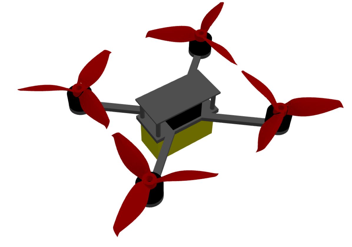
(a) Digital twin of NF1

(b) NF1

Figure 5$\cdot$2: Digital twin of NF1 compared to real quadcopter.

The frame geometry is particularity important as it affects the aircraft’s flight performance. In modern UAV flight controllers, asymmetries in the placement of actuators is accounted for through mixing which is essentially a lookup table that scales the control signal depending on the distance the motor is from each axis of rotation. For RL synthesized controllers, the agent will learn the geometry of the frame and encode this into the NN.

The mass of each individual part of the quadcopter was measured. We then used Numpy-STL [Hattem, 2019] to compute the volume and mass properties for each part, including the center of mass (CoM) and the moments of inertia, $I^{\prime}$. As documented by Gazebo [ine, 2019], the computed moments of inertia must be scaled by the length units (unit_scale), and the density to derive the actual inertia tensor $I$,

$$I=I^{\prime}\text{unit\_scale}^{2}m/V$$ (5.1)

The individual aircraft parts, and their corresponding mesh and mass properties are added to a single SDF file. The position of each aircraft part is then adjusted by modifying the pose XML element to correctly assemble the aircraft. Loading the model in Gazebo, we were able to validate the position of all the parts. When assembling the aircraft, it is essential to make sure the aircraft aligns with the correct axis of rotation, otherwise the IMU will not report the expected values (discussed in detail the following section). In Gazebo the axis lines, (R)ed, (G)reen, and (B)lue, map to the axis (R)oll, (P)itch and (Y)aw respectively. This SDF file also includes the GymFCv2 plugin definition provided in Listing 1.

We obtain the center of thrust value by measuring offset from the bottom of the model to the base of the rotor. In the follow sections we discuss our method for configuring the motor model and IMU plugins which will also be added to the SDF.

5.2.2 IMU Model

To model the IMU we ported over the IMU plugin provided by PX4 [px4, 2019], and implemented the digital twin API. For angular velocity measurements, essentially all this plugin does is query the Gazebo API for the angular velocity for a particular link in the world. Thus the IMU plugin must be configured with a link that will emulate the flight control stack on the real quadcopter. We assigned it to our FC stack link, however one must pay special attention to validate the orientation of the part. If assembled according to the procedure in the previous section, there should be no problems. However this can be confirmed using the test scripts included with GymFCv2 to step the simulator with specific control signals to rotate the aircraft while monitoring the IMU values provided by the plugin. For example, set $u=[0,0,1,1]$ to roll right, the IMU values should match this movement.

In order to increase the fidelity of our digital twin, we introduce gyro noise. In past literature [Jakobi et al., 1995, Andrychowicz et al., 2018, Molchanov et al., 2019] noise has been sampled from a Gaussian distribution. To introduce noise into the model we must identify the gyro noise mean and variance for each axis, $\eta_{(\phi,\mu)}$, $\eta_{(\phi,\sigma)}$, $\eta_{(\theta,\mu)}$, $\eta_{(\theta,\sigma)}$, $\eta_{(\psi,\mu)}$, and $\eta_{(\psi,\sigma)}$.

We would like to point out that we introduce gyro noise during training from within our environment interface user module, not from within the IMU plugin. This provided us with additional flexibility such as easily evaluating the performance of controllers with different noise parameters than having to modify the SDF file to make these changes. In the future we will explore ways to make noise configuration easier for the plugin.

5.2.3 Motor Model

In this section we will discuss our method for developing the motor model for NF1. In Gazebo, model dynamics are implemented by C++ plugins. Each plugin definition is associated with a set of configurable options that are defined in the models SDF file. Our motor models are based on the PX4 Gazebo SITL motor model plugins [px4, 2019] that have been ported to GymFCv2. We have made our motor plugins open source at the following link [Koch, 2019a] allowing the community to utilize them in their own research and improve upon them. In this section we discuss the values that must be configured in the plugin, and the methodology for deriving the values in order to use the motor model plugins. Given the modular architecture of GymFCv2, researchers can also easily use their own motor models.

The PX4 motor models derive force and torque approximations for a propeller propulsion system using blade element theory [McCormick, 1995]. The propeller performance can be defined by two dimensionless coefficients $C_{T}$ and $C_{Q}$ for the thrust and torque coefficient respectively. The thrust coefficient is given as,

$$C_{T}=\frac{T}{\rho n^{2}D^{4}}$$ (5.2)

where $T$ is the thrust, $\rho$ is the air mass density, $n$ is the propeller rotational speed in revolutions per second, and $D$ is the propeller diameter. The torque coefficient is given as,

$$C_{Q}=\frac{Q}{\rho n^{2}D^{5}}$$ (5.3)

where $Q$ is the torque. The values for $T$, $Q$, $\rho$, and $D$ must have consistent units.

The thrust and torque coefficients are a function of the dimensionless advanced ratio $J$ which quantifies the effects of the propeller in forward motion in relation to its angular velocity given by,

$$J=\frac{V_{\infty}}{nD}$$ (5.4)

where $V_{\infty}$ is the freestream fluid velocity. When $J=0$, this is the static case in which $V_{\infty}=0$.

To develop a model for a propeller driven propulsion system to be used in simulation, an approximation of the thrust and torque for a given propeller rotational speed must be derived. The PX4 Gazebo SITL plugin computes the motor thrust in Netwons (N), for each motor by,

$$T(\omega)=\omega^{2}K_{T}$$ (5.5)

which is a function of the rotor’s current angular velocity, $\omega$, in radians per second for a configurable thrust constant $K_{T}$. Given $C_{T}$, one can derive the constant $K_{T}$ to be,

$$K_{T}=\frac{C_{T}\rho D^{4}}{(2\pi)^{2}}$$ (5.6)

where $\rho$ is in $\text{kg/}\text{m}^{3}$ and the propeller diameter $D$ is in meters. The PX4 Gazebo SITL plugin computes the torque in Newton meters ($N\cdot m$) as a function of the thrust,

$$Q(T)=TK_{Q}$$ (5.7)

where $K_{Q}$ is a configurable torque constant. Given $C_{T}$ and $C_{Q}$, $K_{Q}$ is defined as follows,

$$K_{Q}=\frac{C_{Q}D}{C_{T}}$$ (5.8)

The PX4 SITL motor model requires us to find $C_{T}$ and $C_{Q}$ experimentally for $J=0$ in order to calculate the constants $K_{T}$ and $K_{Q}$ .

Motor Response. In addition to modelling the thrust and torque of the propulsion system, we also need to model the motor response for a given control input. Most research related to quadcopter control do not model the motor response and assume the motor response to be instant, which can lead to inaccuracies [Molchanov et al., 2019].

For a known maximum rotational velocity, which is found experimentally, a PID controller can be used to model the motor response. We found this to provide a more realistic response than other methods, such as a discrete first order filter used by the PX4 SITL motor model. The PID controller computes the additive force $F(t)^{\prime}$ at time $t$ to apply to the rotor as follows,

$$F(t)^{\prime}=K_{p}e(t)+K_{i}\int_{0}^{t}e(\tau)d\tau+K_{d}\frac{de(t)}{dt}$$ (5.9)

where the error is defined as,

$$e(t)=\omega(t)-\omega(t)^{*}$$ (5.10)

which is the difference between the current rotor angular velocity $\omega(t)$, and desired rotor velocity $\omega(t)^{*}=H(u)$. Here, $H$ is the rotor velocity transfer function which is necessary to create the mapping $u\rightarrow\omega^{*}$ as there may not be a linear relationship between the control signal and the motor angular velocity.

To control the acceleration and deceleration of the motor response the output of the PID controller is clamped to a minimum value $F_{\text{min}}$ and maximum value $F_{\text{max}}$. Essentially these values control the slope of the response.

$$F(t)=\text{clamp}(F(t)^{\prime},F_{\text{min}},F_{\text{max}})$$ (5.11)

The clamped force $F(t)$ is then added to the propeller joint in the Gazebo simulator. The three PID gains, $K_{P}$, $K_{I}$, and $K_{D}$ along with $F_{\text{min}}$, $F_{\text{max}}$ must be tuned to achieve the desired step response.

In summary, to configure the motor model plugin we must derive the constants $K_{T}$, $K_{Q}$, $H$, $K_{P}$, $K_{I}$, $K_{D}$, $F_{\text{min}}$, and $F_{\text{max}}$ through experimental measurements. In the following section we will discuss our methodology for obtaining these values.

5.2.4 Experimental Methodology

In this section we introduce our experimental methodology for deriving the motor model configuration constants which requires specially designed equipment and procedures to obtain. For the IMU model, we did not require any special equipment or procedures to derive the values for our model.

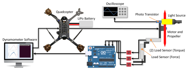
Figure 5$\cdot$3: Dynamometer diagram.

Equipment

To derive the motor constants defined in Section 5.2.3 we constructed a dynamometer (dyno) to measure thrust, torque and rotor angular velocity. A diagram of our system is illustrated in Fig. 5$\cdot$3. Our custom dyno software consists of two modules that run in parallel. The first module controls the motor and the second module captures and records sensor data. Our motor control module uses a unique approach in which the electronics from the aircraft are repurposed for controlling the speed of the motor. A complete build log, including the electronics of our aircraft, can be found at [rot, 2018]. This solution is cost effective and reduces any errors that may be introduced if using a dyno that uses hardware that differs from that found in the aircraft (e.g., latency caused by ESC protocols, power delivery of the ESC, etc.). The flight controller ran the Neuroflight firmware and our ESC uses the firmware BLHeli_32. The motor control module sends motor commands to the aircraft’s flight controller via the MultiWiiSerial (MSP) protocol over USB. The flight controller interprets the MSP command and writes the motor command to the ESC which applies the necessary power to achieve the desired output to the motor.

The sensor data capture module interfaces with an Arduino which is responsible for aggregating the sensor data obtained from the motor. The motor is mounted to a static testing apparatus from RCBenchmark [rcb, 2019] that is outfitted with the sensors to collect thrust, torque and rotor velocity measurements. The motor mount is attached perpendicular to two 1Kg load sensors that are separated from one another by 80mm for measuring torque. The torque is calculated from the average of the two load sensors $\text{LS}_{\tau_{1}}$ and $\text{LS}_{\tau_{2}}$ using the following equation,

$$\tau=\frac{|k_{\tau_{1}}\text{LS}_{\tau_{1}}|+|k_{\tau_{2}}\text{LS}_{\tau_{2}}|}{2}$$ (5.12)

where $k_{\tau_{1}}$ and $k_{\tau_{2}}$ are constants found during calibration. The absolute value of each is taken as one load sensor will experience a pull (outputting a negative value), while the other will experience a push (outputting a positive value).

The load sensors for measuring torque is attached perpendicular to a 2Kg load sensor $\text{LS}_{T}$ for measuring thrust. The resulting force is calculated by,

$$T=|k_{T}\text{LS}_{T}|$$ (5.13)

where $k_{T}$ is a constant found during calibration. The absolute value is taken to support both push and pull propellers. Each of the load sensors is connected to an amplifier to boost the signal to be read by the Arduino.

To measure rotor angular velocity, a photo transistor and a light source is used which triggers a pulse every time a propeller blade passes between the transistor and light source. Our first approach attempted to connect the output of the photo transistor to an interrupt pin on the Arduino which would cause a interrupt handler to be invoked every time a blade passed the photo transistor and light source. Based on the number of interrupts that occur within a predefined time window, the RPM could then be calculated. This approach was ideal as it would allow the entire system to be automated. However during validation using a Tektronix MDO3034 oscilloscope we found the readings from the Arduino were limited to about 75% throttle. Upon further inspection we discovered as the angular velocity increased, the voltage emitted from the sensor would decrease. This drop in voltage was enough to be below the $0.6\text{Vcc}$ threshold for what is considered a logic high on the Arduino. Due to this limitation, we decided to manually collect the velocity data using the oscilloscope which also has the added benefit of having a higher sampling rate. Using the oscilloscope, the voltage values were recorded during each measurement. Post processing of the data is performed to derive the RPM values. This is accomplished by parsing every $b=3$ voltage pulse as a single rotation. The RPMs were then calculated by the intermediate times between each complete propeller rotation.

Dynamometer simulator. To validate and develop our motor model, we used GymFCv2 to implement a dyno simulator to measure the motors thrust, torque, and RPMs in simulation. The dyno architecture is depicted in Fig. 5$\cdot$4. A motor model was created extracting the motor and propeller links used in the NF1 model. The aircraft configuration enabled the ESC sensor to obtain the thrust, torque, and RPMs measurements. A dyno software module interfaces with GymFCv2 to replicate the control inputs provided by the real dyno. At every simulation step the dyno module records the measurements and at the end of the simulation saves the data to a file for later processing. This dyno software is open source and is available from the GymFC code repository [Koch, 2018a].

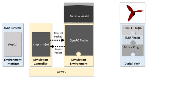
Figure 5$\cdot$4: Instance of GymFCv2 architecture for dyno validation.

Calibration

Calibration of the dyno was required to obtain accurate thrust and torque measurements from the load cells. For torque calibration, a lever 130mm in length was mounted to the center of the motor mounting plate, extending to the left, to allow torque to be applied to the motor mounting plate. Payloads starting at 200 grams were hung from the lever in increments of 200 grams until the max rating of the load sensor was reached. Both calculated torque load sensor readings were recorded. Once a measurement was recorded for a given payload, the payload was removed before the next incremented payload was measured to check for hysteresis. This process was then repeated with the lever extending to the right. A linear fit was then applied to each of the load cell data to derive a transfer function for each load cell torque measurements.

For thrust calibration, the dyno was rotated 90 degrees counter clockwise such that the motor mounting plate faced upward. Payloads were then added on top of the motor mount thus applying a positive force on the force load sensor. The sensor recording procedure was conducted in the same manner as the torque calibration and a linear fit was also then applied to the sensor data to derive a transfer function for thrust measurements.

Procedure

Using the dyno we have designed two experiments to measure and collect the necessary data to derive the motor model constants. The first experiment performs a step response and the second experiment performs a throttle ramp.

The step response experiment is conducted to identify the motor response parameters (i.e., $H$, $K_{P}$, $K_{I}$, $K_{D}$, $F_{\text{min}}$, and $F_{\text{max}}$). To perform these measurements a fixed throttle value is applied for one second to capture the acceleration, followed by a throttle value of zero for another additional second to capture deceleration. Four target throttle values are selected: 25%, 50%, 75%, and 100%.

Using the captured step response data, a throttle curve is generated to identify the relationship between the control signal (i.e., throttle value) and the corresponding achieved rotor velocity. This data is fitted to a polynomial function to derive the rotor velocity transfer function $H$.

Once the control signal to rotor velocity mapping is modelled to derive $H$, the dyno simulator can then be used to manually tune the motor model PID controller to fit the measured step response. We can do this independently of having a complete motor model because we are only interested in the rotor velocity and its response, not of its thrust and torque output.

The motor model plugin configuration is first updated with $H$. The $K_{P}$ term is then incremented until the desired target velocity was reached, while $F_{\text{min}}$ and $F_{\text{max}}$ are tuned to match the slope during acceleration and deceleration. If we recall from Section 5.2.3 the reason $F_{\text{min}}$ and $F_{\text{max}}$ cannot be computed directly from the experimentally measured slope is due to the fact that the output of the PID controller sets the accumulated force on the rotor, not the absolute RPM velocity of the rotor. In this work we set $K_{I}$ and $K_{D}$ to zero.

The throttle ramp experiment is used to measure the torque and thrust. The throttle ramp increments the throttle from 0 to 100% over the course of 20 seconds and then decrements the throttle from 100% to 0 for an additional 20 seconds. Using the maximum rotor velocity obtained from the step response experiment, the maximum thrust and torque values are used to calculate $K_{T}$, and $K_{Q}$.

With all of the constants identified and updated in the motor model plugin configuration, the dyno simulator is used to validate the motor model plugin against the real world measured data.

5.2.5 Experimental Results

In this section we report our empirical experimental results. Our gyro noise parameters are summarized in Table 5.2. The parameters obtained from the motor experimental measurements are summarized in Table 5.3 while the derived motor constants are summarized in Table 5.4.

Axis (ax)	Mean ($\mu$)	Variance ($\sigma$)
Roll ($\phi$)	-0.2546	1.3373
Pitch ($\theta$)	0.2419	0.9990
Yaw ($\psi$)	0.079	1.4516

Table 5.2: Normal PDF parameters for gyro noise mean ($\eta_{(\text{ax},\mu)}$) and variance ($\eta_{(\text{ax},\sigma)}$) in degrees per second.

Parameter	Value
Max $T$	6.59 $\pm$ 0.09 N
Max $Q$	0.0565 $\pm$ 0.0008 N $\cdot$ m
Max RPM	25042 RPM
$C_{T0}$	$2.87\times 10^{-2}$
$C_{Q0}$	$1.38\times 10^{-3}$

Table 5.3: Propeller propulsion system parameters.

Parameter	Value
$K_{T}$	$9.37\times 10^{-7}$
$K_{Q}$	$8.64\times 10^{-3}$
$K_{p}$	0.0001
$K_{i}$	0
$K_{d}$	0
$F_{\text{min}}$	-0.1
$F_{\text{max}}$	0.05
$H$	Eq. 5.14

Table 5.4: Propeller propulsion system model constants.

Gyro Noise

To obtain the parameters for they IMU noise model we recorded the gyroscope values from our real aircraft, NF1, when armed, for over 30 seconds to obtain 26,777 samples. We then plotted a histogram of the data for each axis. These plots are displayed in Fig. 5$\cdot$5. As we can see from the figure, we verify the data fits well to a normal distribution. Next we fit the data to the normal distribution probability density function (PDF) to obtain the mean and variance values for each axis as reported in Table 5.2.

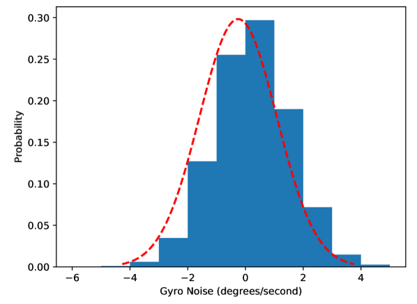
(a) Roll

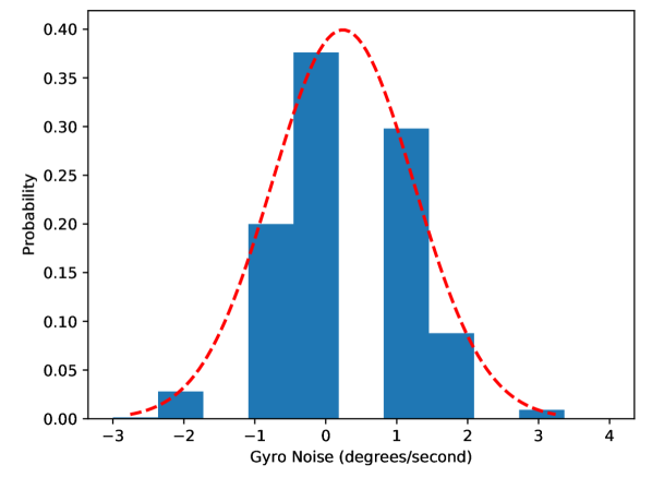
(b) Pitch

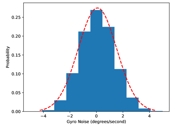
(c) Yaw

Figure 5$\cdot$5: Gyro Noise

Step Response

Results from the step response experiment are displayed in Fig. 5$\cdot$6 while the throttle curve is displayed in Fig. 5$\cdot$7 which is fitted to a two degree polynomial function to obtain the transfer function defined in Eq. 5.14.

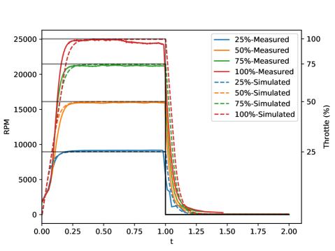
Figure 5$\cdot$6: Step response of motor model compared to real motor.

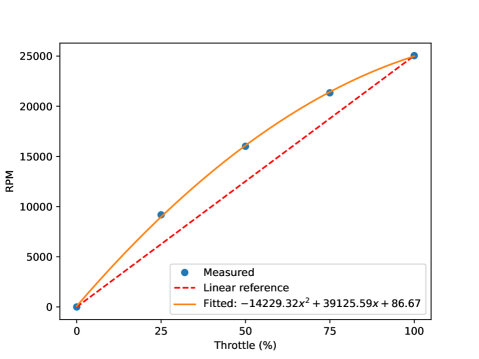
Figure 5$\cdot$7: Throttle curve.

$$H(u)=-14,229.32u^{2}+39,125.59u+86.67$$ (5.14)

These results signify the importance of using the ESC (and ESC firmware) used during flight for deriving the motor measurements in order to generate an accurate model. Each propulsion system will result in a unique motor response due to the current drawn for a given propeller and the capabilities of the ESC to delivery this power to the motor. Most ESC firmware for UAVs use an open-loop controller, that is, there is no feedback to reach its target. Unlike our simulated propulsion system, the real ESC is unaware of the maximum achievable rotor velocity as this will vary depending on the motor and propeller combination. The ESC will map the control signal to a duty cycle (i.e., switching frequency) to reach a particular angular velocity. It is up to the higher level attitude controller to compute the control signals to send to the ESC in order achieve the desired aircraft angular velocity.

After updating the motor model plugin configuration with the identified transfer function, the motor PID controller was tuned to obtain the desired motor response. Fig. 5$\cdot$6 also shows a comparison of the measured step response with the motor model plugin validated in simulation. Our analysis finds each simulation step response to have an angular velocity percent error (i.e., the MAE divided by the max RPMs) of 4.11%, 3.51%, 3.31% and 3.90% for the 25%, 50%, 75%, and 100% throttle values respectively. These results show the motor response of the digital twin is accurate to less than 5% error of the real motor response across all throttle values tested.

Throttle Ramp

We performed $N=20$ independent measurements and report the maximum thrust and torque values along with the 95% confidence interval in Table 5.3. Additionally, the data was averaged together to generate the thrust response displayed in Fig. 5$\cdot$8(a) and the torque response is displayed in Fig. 5$\cdot$8(b). In these figures, the dashed black line is the percent throttle value applied.

(a) Thrust

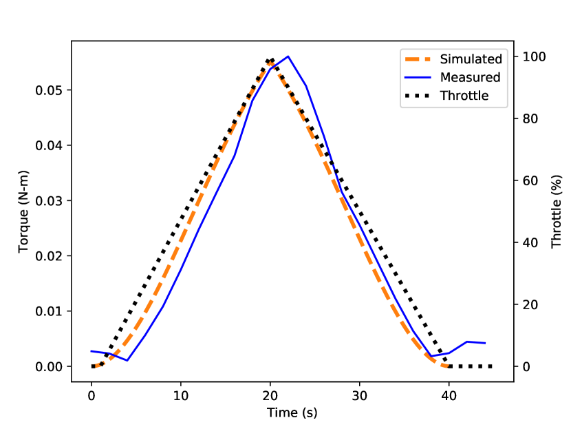
(b) Torque

Figure 5$\cdot$8: Throttle ramp measurements.

Motor Constants and Validation

Using the motor parameters found during experimentation we first derived the thrust and torque coefficients and then use these to calculate the motor constants. The thrust and torque coefficients in relation to the motor velocity is displayed in Fig. 5$\cdot$9 while the thrust and torque motor constants in relation to the motor velocity is displayed in Fig. 5$\cdot$10.

The motor model plugin configuration is completed with addition of the derived motor constants providing the thrust and torque dynamics in simulation. With the completed model, we are able to validate the model using the dyno simulator and compare the results to the experimental measured data. For thrust and torque these results are displayed in Fig. 5$\cdot$8. The results are comparable. We find the motor model to have an MAE of 0.003 N $\cdot$ m for the torque output compared to the real motor measurements, and an MAE of 0.588 N for the thrust output.

The real measurements do experience a greater delay however this is likely attributed to the use of static motor constants where we can visually see in Fig. 5$\cdot$10 the constants, as a function of the rotor velocity, are not only not static, but nonlinear.

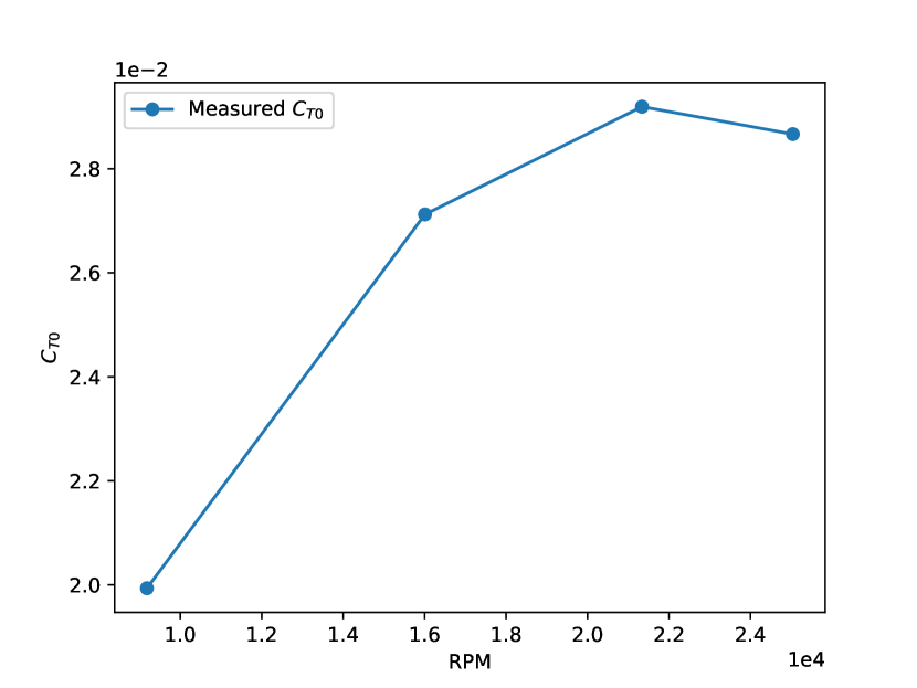
(a) Thrust coefficient

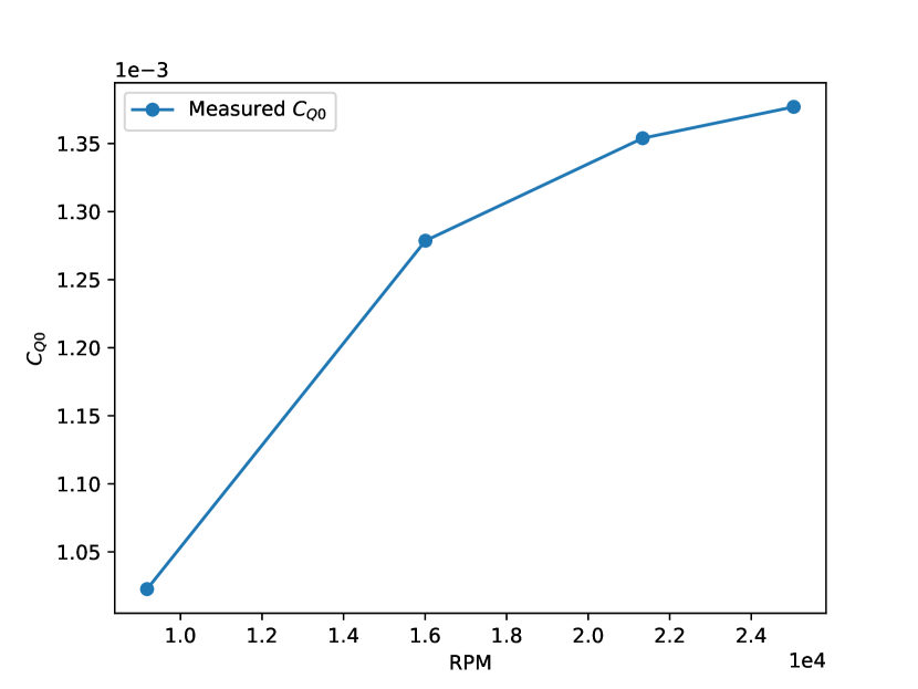
(b) Torque coefficient

Figure 5$\cdot$9: Propeller coefficients

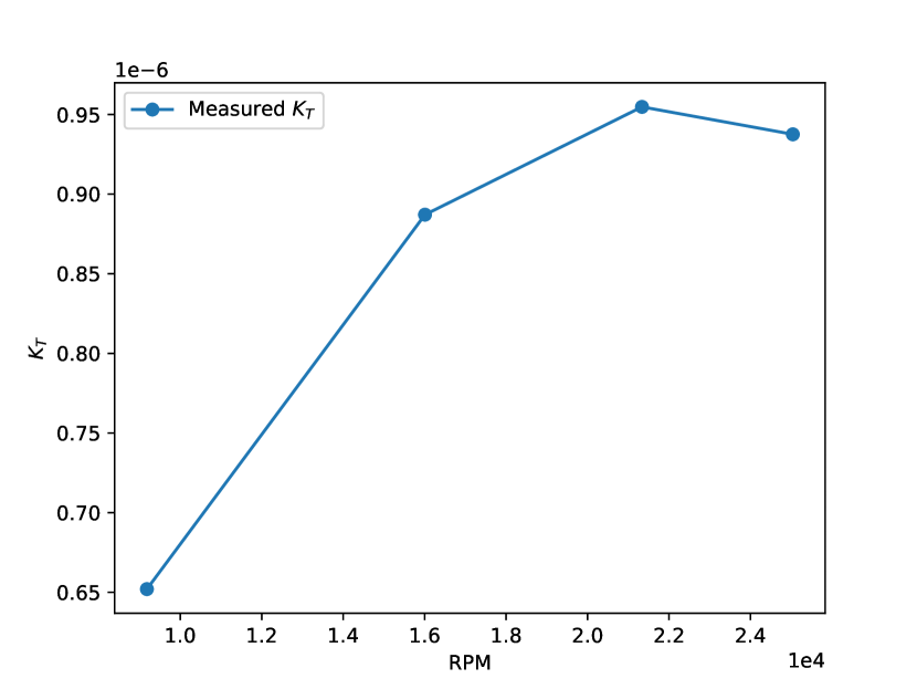
(a) Thrust constant

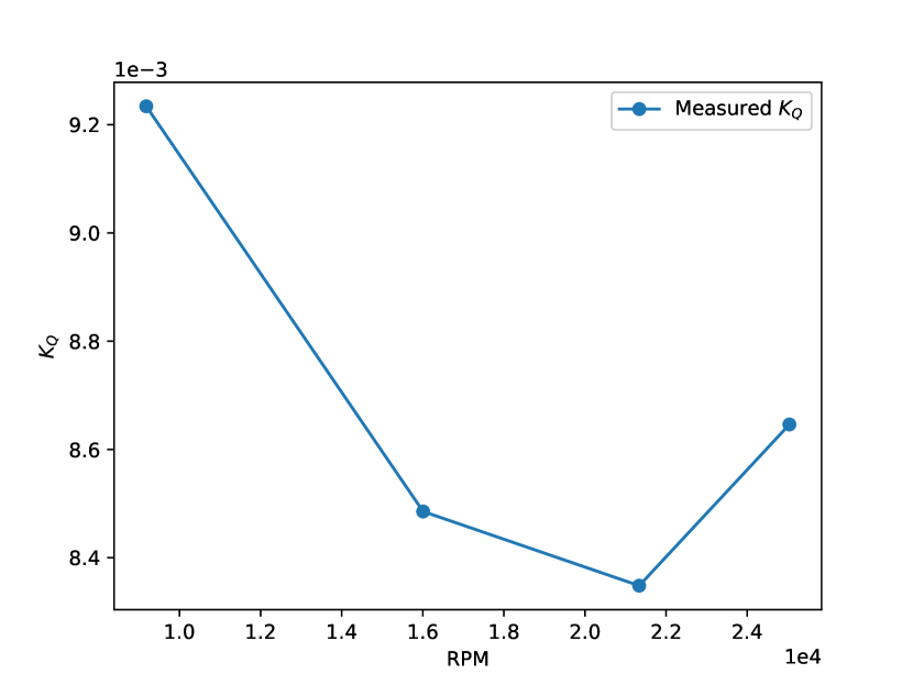
(b) Torque constant

Figure 5$\cdot$10: Motor model constants.

5.3 Simulation Stability Analysis

Multirotors capable of achieving high angular velocities, which induce large centripetal forces, are at risk of becoming unstable during simulation. The problem is exaggerated as the number of links in a model increase. The root cause of the simulation instability is due to the type of coordinate solver used by the physics engine. Generally speaking, a physics engine’s coordinate solver can be categorized as either a maximal coordinate solver or a generalized coordinate solver (also know as reduced coordinates) [Coumans, 2014]. A maximal coordinate solver treats each body (link) as a separate rigid body with 6 degrees of freedom (3 for position and 3 for orientation). Constraints are then used to connect bodies and enforce the intended degrees of freedom. Because the bodies are not represented as a single entity this solver is known to cause bodies to drift due to coordinate redundancies and inaccuracies enforcing constraints. On the other hand, a generalized coordinate solver represents the bodies only by the degrees of freedom.

The Gazebo simulator supports the following physics engines: ODE [Smith, Russel, 2006], Bullet [Coumans, 2015], Simbody [Sherman et al., 2011] and DART [Lee et al., 2018]. ODE, the default physics engine for Gazebo, uses a maximal coordinate system while DART advertises its self as being accurate and stable due its use of generalized coordinate solver.

In this section we evaluate the stability our model using both the ODE and DART physics engines as a precursor for establishing which will be necessary to use for flight controller synthesis.

5.3.1 Measuring Stability

In this section we describe our algorithm Alg 1 we developed for measuring the simulation stability of our aircraft model. In summary, this algorithm measures the stability metric $\delta$ defined as the sum of the absolute value differences between the current distances of the bodies from their initial state at each time step of the simulator (defined at line 8). The simulation is considered unstable is there occurs any drifting between the bodies (i.e., $\delta>0$).

As the forces between the bodies becomes more complex, the simulation becomes more likely to become unstable. Thus we must measure $\delta$ for a range of angular velocities starting from still to its maximum achievable angular velocity of the aircraft. To perform this measurement, we assume this is a precursor to developing the flight controller therefore the idea is to excite each motor permutation to reach a variety of angular velocities. More specifically we set each action $A$ (i.e., control signal set) of the total possible $2^{\text{M}}$ permutations ($\sigma$) where $M$ is the total actuator count of the aircraft and each motor control signal can either be off, $0$, or full throttle $1$. After each time step $t$, the simulator receives the current state $S$ which contains the aircraft’s current angular velocity $\Omega$ for each roll, pitch and yaw axis. We also obtain the set of all the aircraft’s individual links relative positions $V(t)$. We can think of the links as a undirected weighted graph where each link position is a vertex and the edge weight is the relative distance from one link to the other. Using the set of vertices we calculate a Euclidean distance matrix $D(t)_{i,j}$ for each of the $i$, $j$ link combinations. The stability metric is then calculated using this distance matrix and added to the result vector $Y$. One can then use $Y$ to find at which velocities the simulation is stable for.

Inputs : A GymFCv2 environment $E$ with the aircraft model to be measured.

Returns : A vector $Y$ where each element is a tuple of the stability measurement $\delta$ at the corresponding angular velocity $\Omega$.

1

2$Y\leftarrow\emptyset$

3

4for  $A\in\sigma$ do

5       while $t=1,2,\dots$  do

6             $S\leftarrow E.Step(A)$

7             $\Omega\leftarrow GetAngularVelocities(S)$

8             V(t) = GetBodyPoses(t)

9             $D(t)_{i,j}$ = EuclideanDistanceMatrix(V)

10             $\delta\leftarrow\displaystyle\sum_{i=0}^{N-1}\displaystyle\sum_{j=0}^{N-1}|D(t)_{i,j}-D(0)_{i,j}|$

11             $Y\leftarrow Y+\{(\delta,\Omega)\}$

12            

13      

14return Y

Algorithm 1 Model Stability Measurement

5.3.2 Implementation

To implement this algorithm we used GymFCv2 to issue the actions to the aircraft and wrote a script (available in GymFCv2) using py3gazebo[Koch, 2019b] to interface with Gazebo’s messaging API. This interface is based on a publish-subscribe architecture allowing the client to subscribe to a number of events. Our script implements the GetBodyPoses function (Alg. 1 line 6) by subscribing to the poses_stamped messages which contains an array of the model links and their corresponding positions $V(t)$. The stability metric results $Y$ are then used to generate 3D plots to visualize the stability of the model.

5.3.3 Stability Results

We evaluated the stability of our model using Gazebo’s default physics engine ODE with various simulation step sizes, and compared this to DART. Our results for ODE using step sizes of 2ms (500kHz), 1ms (1kHz), and 500$\mu s$ (2kHz) are displayed in Fig. 5$\cdot$11, Fig. 5$\cdot$12, Fig. 5$\cdot$13 respectively. Results for DART are displayed in Fig. 5$\cdot$14.

These simulation results show the execution of each of the motor permutations and the angular velocity that is achieved. A heat map is used to indicate the value of $\delta$ in meters for the corresponding angular velocity. As we can see the ODE physics engine with the maximal coordinate solver results in a very unstable simulation environment. For the largest step size of 2ms, bodies start to separate at as low as $\Omega=[-87,85,147]$ degrees per second with a max separation of 95mm. As the step size decreases (i.e., simulation rate increases), stability increases as the physics engine is able to calculate the state more frequently. At a step size of 1ms, instability begin to occur at $\Omega=[-263,269,364]$ degrees per second with a max separation of 39mm and at a step size of 500$\mu$s bodies begin to separate at $\Omega=[-617,428,693]$ degrees per second with a max separate of 10mm. Now if we refer to Fig. 5$\cdot$14 we can see that by using a generalized coordinate solver (i.e., DART) zero drifting occurs. Thus in summary, we find stability can be accomplished by two methods:

1. If using ODE or a maximal coordinate solver, decrease the step size until the minimum angular velocity in which body separate occurs is greater than the flight envelop of the aircraft.

2. Use a physics engine with a generalized coordinate solver such as DART. It is recommended to use this option unless there is a specific reason in which this solver can not be used.

Based on these findings GymFCv2 has DART enabled by default.

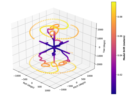
Figure 5$\cdot$11: ODE physics engine with $2ms$ step size (500Hz).

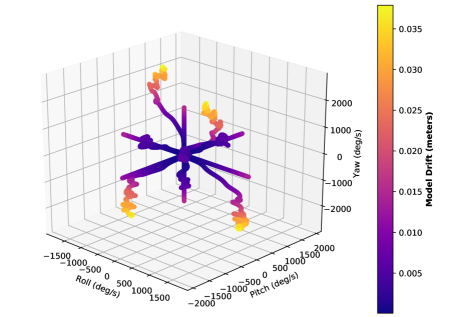
Figure 5$\cdot$12: ODE physics engine with $1ms$ step size (1kHz).

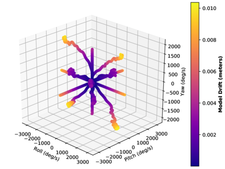
Figure 5$\cdot$13: ODE physics engine with $500\mu s$ step size (2kHz).

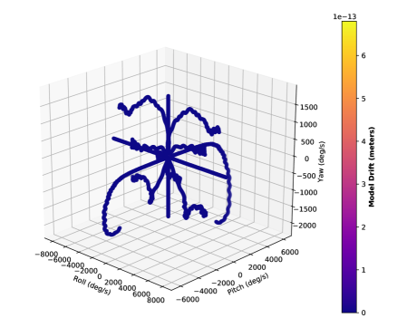
Figure 5$\cdot$14: DART physics engine with $1ms$ step size (1kHz).

5.4 Neuro-flight Controller Training Implementation

In Section 5.2 we discussed in great detail our methodology for creating a multicopter digital twin, one of the user provided modules. In this section we will discuss our implementation of the remaining user supplied modules to be used with GymFCv2 for synthesizing a neuro-flight controller via RL.

5.4.1 User Provided Modules

Control Algorithm and Tuner

We use a neural network with the same architecture as in Chapter 4 with the only difference being the number of hidden nodes has increased from 32 to 64. Increasing the size of the network further did not provide any additional performance benefits.

Similar to Chapter 4 we trained using the PPO1 implementation from OpenAI Baselines. We did put in a considerable amount of effort migrating to Tensorforce [Schaarschmidt et al., 2017] in order to experiment with the beta distribution and LSTM networks, however we could not reach even close to the level of performance we could with OpenAI Baselines. This was even after using a hyperparameter tuning [Falkner et al., 2018]. The primary challenge was due to the lack of documentation and using hyperparameter definitions that differ from the original PPO paper [Schulman et al., 2017]. An additional reason could be due to the differences in implementations of the algorithm, which prior research has shown to greatly affect performance [Henderson et al., 2018]. We did find that we needed to increase the step size to $1\times 10^{-3}$ when using the beta distribution, yet this was still not enough to match the performance provided by OpenAI Baselines.

For tuning (i.e., training) the NN we used the hyperparameters defined in Table 5.5. The horizon and batch size were slightly increased from Chapter 4.

Hyperparameter	Value
Horizon (T)	512
Adam stepsize	$1\times 10^{-4}\times\rho$
Num. epochs	5
Minibatch size	64
Discount ($\gamma$)	0.99
GAE parameter ($\lambda$)	0.95

Table 5.5: PPO hyperparameters where $\rho$ is linearly annealed over the course of training from 1 to 0.

Environment Interface

To support RL training, our environment interface implements an OpenAI Gym, to provide an interface for the PPO algorithm. The environment interface implements the OpenAI Gym functions, step, and reset. The step function makes a call to four important functions we have implemented for our training environment: transform_input, transform_output, generate_command and compute_reward. The functions transform_input and transform_output support transforming the aircraft state to the NN input, and the NN output to the control signal, respectively. The function generate_command generates the angular velocity setpoint for each axis of rotation the agent must achieve for the given time step. Lastly, the compute_reward function calculates the reward for the agent at each time step. In the remainder of this section we will discuss each function in detail.

Transformation functions. The transform_input function takes as input the aircraft state, $S$ which contains the angular velocity $\Omega$ and the desired angular velocity $\Omega^{*}$, and computes the network input as defined in Eq. 4.3.

The transform_output functions scales and adds a bias to the NN output $y$ to derive the control signals $u$ in the range $[0,1]$ required by the Neuroflight firmware. Because the output of the NN is the mean from the Gaussian distribution, the output is first clipped to the action bounds $y_{\text{low}}=-1$ and $y_{\text{high}}=1$. Next the scaling and bias is performed, where $u_{\text{low}}=0$, and $u_{\text{high}}=1$,

$$y =\text{clip}(y,y_{\text{low}},y_{\text{high}})$$ (5.15)

$$u =\frac{(u_{\text{high}}-u_{\text{low}})(y-y_{\text{low}})}{(y_{\text{high}}-y_{\text{low}})}+u_{\text{low}}$$ (5.16)

Command generation. The generate_command function computes the angular velocity setpoint. The objective of the agent is to reach this setpoint. From Chapter 4 we found that is was important to expose the agent to, not only acceleration, but also deceleration for transferring the agent to the real world. Thus GymFCv1.5 continuously generates new commands until a predefined time out is reached. However, with such a long episode, analyzing the individual step response caused by the change in the command input increases in complexity as you have to slice the episode into the individual pulses before analyzing. Additionally, during early stages of training, the agent can get the aircraft into extremely fast angular velocities, well exceeding the target, which is undesirable to allow this behavior to last the entire episode.

To address these concerns, this command generator simplifies the environment to only a single pulse. We begin by setting $\Omega^{*}=[0,0,0]$ for half a second. This allows the agent to learn its idle or hover state. A command is then randomly sampled and held for two seconds which teaches the agent to accelerate to a desired angular velocity, followed by a steady state. The command is then set back to $\Omega^{*}=[0,0,0]$ for an another additional two seconds to teach deceleration. The question becomes, what is the best distribution to sample the setpoints from? In previous chapters we sampled from uniform random, however through our experience, the agent will perform best through its sampled range. It is more desirable to be accurate within the flight envelop than extreme cases.

To discover the underlying command input distribution, we obtained a total of 786,022 pilot input commands, from real test flights, and created a histogram with 20 bins. Results are show in Fig. 5$\cdot$15 for each axis, while a dashed red line is a fitted to a normal distribution PDF. As we can see the command inputs roughly fit a normal distribution with an average control input of -2.3 deg/s with a standard deviation of 12.4 deg/s. The average command input, centering around zero degrees, was expected. This is because the majority of the time during flight a heading is maintained in which the angular velocity changes very little. Minor adjustments may be made to compensate for external disturbances acting upon the aircraft. The variance will be correlated to the type of flying performed. For example, frequent aggressive aerobatic maneuvers would use a greater range of the flight envelope resulting in a wider variance, while more conservative tasks, such as aerial photography and video would result in a narrower variance. Based on these results, the command generation function samples from a normal distribution with $\mu=0$, however we increase the standard deviation to $\sigma=100$ because we want to evaluate the performance performing aggressive maneuvers on the edge of the flight envelope.

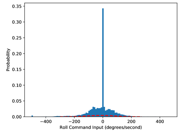
(a) Roll

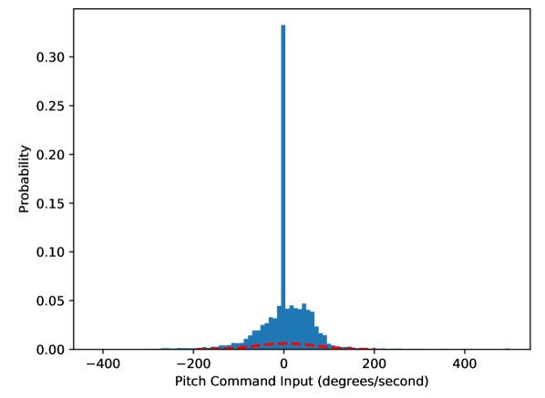
(b) Pitch

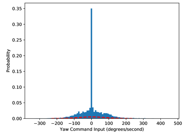
(c) Yaw

Figure 5$\cdot$15: PDF of Pilot Command Inputs

Reward function. Our reward function is an improved iteration from Chapter 4 with some additional changes to increase stability. The reward function is defined in Alg. 2 and is called at each time step. In lines 1-4, a reward is given capturing the agents progress to minimizing the error. We found this to provide more stability than the sum of squared errors. At line 5, the agent is penalized for the max changes in the control signal to reduce output oscillations. This is scaled by the constant $\beta>0$. At line 6 and 7, a reward is given to the agent for reducing their average control signal output if they are in an error band defined by the percent $\epsilon$ of the target angular velocity. The remaining penalties, defined in lines 8 to 12, are to help stabilize the learning process and consist of events that should never happen. We define a max penalty high enough such that the agent will not repeat the behavior. We set MAX_PENALTY = $1\times 10^{9}$ however there is some flexibility to this value. Line 8, penalizes the agent for saturating the output. Recall the agents output ($a$), for a stochastic policy, is the mean of a Gaussian distribution. The action is unbounded and thus can exceed the bounds of the control signal. Although this value is clipped during the transformation function, we found without this penalty, the angular velocity of the aircraft would rapidly increase and not come back down. We believe this to be primarily caused by the delayed motor response as the control signal provided by the agent will not immediately result in a change. Lines 9 and 10 penalize the agent if they have saturated all the control outputs which should never happen. While lines 11 and 12 penalize the agent in cases where they do nothing. This penalty is derived from the basic quadcopter dynamics such that at least two motors are required to preform one of desired commands. If more than two motors are zero, and the target angular velocity is not zeros, the penalty is applied.

Returns : Reward $r$ at time $t$

1 $r\leftarrow 0$

2 $r_{e,t}\leftarrow-(e_{\phi}^{2}+e_{\theta}^{2}+e_{\psi}^{2})$

3 $r\leftarrow r+r_{e,t}-r_{e,t-1}$

4 $r_{e,t-1}\leftarrow r_{e,t}$

5 $r\leftarrow r-\beta\texttt{max}(|u_{t}-u_{t-1}|)$

6 if $|e|<\epsilon|\Omega^{*}|$ then

7       $r\leftarrow\alpha\left(1-\bar{u}\right)$

8      

9$r\leftarrow r-\texttt{MAX\_PENALTY}\sum\texttt{max}(a-1,0)$

10 if $\forall u_{i}\in u,u_{i}\equiv 1$ then

11       $r\leftarrow r-\texttt{MAX\_PENALTY}$

12      

13if $2<\sum_{u_{i}\in u:u_{i}\neq 0}1\texttt{~{}and~{}}\exists\Omega_{i}\in\Omega^{*}:\Omega_{i}>0$ then

14       $r\leftarrow r-\texttt{MAX\_PENALTY}$

15      

return r

Algorithm 2 Reward function

5.5 Evaluation

In this section we synthesize a neuro-controller via RL using the GymFCv2 implementation. Most importantly, the evaluations differs from the other evaluations such that the controllers are tuned and evaluated in simulation using our digital twin of NF1.

We evaluate the flight controller in simulation, and also in the real world. As we have done in earlier chapters, we also provide a simulation baseline using a PID controller. Using a PID tuning platform implementation of GymFCv2, we tune our PID controller and compare the performance to that of the neuro-flight controller in simulation.

5.5.1 Neuro-Controller Synthesis

Before training, we disabled gravity in the simulation environment as we did in GymFCv1.5. We did experiment with gravity enabled, and while the agent is able to minimize the error without problem, minimizing the control output and oscillations were more difficult. We believe this is partially explained by less exposure to certain conditions that encourage our desired behavior. In other words, with gravity disabled, we have no additional downward force acting on the aircraft, therefore, in the simulation environment we do not need to care about how the orientation will affect the control of the aircraft. With gravity enabled, if a command puts the aircraft in a state outside of its flight envelope, (e.g., perpendicular to the ground), it will negatively affect training. Thus the only time the agent is exposed to a condition for idle, is at the beginning of episode when the setpoint is zeros. Intuitively we thought adding a quaternion to the NN input would help the agent distinguish between these states however this did not help reduce the control output and oscillations. In future work we will investigate how we can build more stable training environments for when gravity is enabled to create a more realistic training environment.

Using our RL implementation of GymFCv2, we train our NN for 10 million time steps with the architecture and hyperparameters defined in Section 5.4.1. Training was conducted on a desktop computer running Ubuntu 18.04 with an eight-core i7-7700 CPU and an NVIDIA GeForce GT 730 graphics card.

During training, every 100,000 steps, a Tensorflow checkpoint of the policy is saved. In parallel, a monitoring program watches for new checkpoints. The monitoring program allows for the training progress to be monitored and evaluation of the performance of the controller. This is helpful during reward engineering to identify if the rewards are doing what we actually intend them to do and identify trends. If we recall from Section 4.3.2, during training the output of the NN is stochastic to aid in exploration. However when deployed, we use the deterministic output of the NN. The monitoring program evaluates each checkpoint, deterministically, for a total of five episodes.

Fig. 5$\cdot$16 displays the results of the checkpoint validations throughout training for four metrics. The plots report the average metrics for each checkpoint indicated by the black line, while the red regions define the min and max values experienced for each metric. The first subplot reports the mean absolute error represented by $|e|$. The second subplot is the average control output $u$, while the third subplot is the average change in the control output $\Delta u$. Last we have the average reward $r$ the controller would have received during training (remember this is validation, not training).

From the validation plot we can see the agent first minimizes the error which, in turn, accumulates the majority of the reward. This happens very quickly and consistently, within one million time steps. Once the error has been minimizes, and the agent is in the error band, the agent begins to accumulate more reward for minimizing the control output. Minimizing the control output, also helps to reduce high amplitude oscillations and reduce the output oscillations. As we can see by the increase in red, there is more variation in the change to the control signal. Developing a reward system to balance the control output effort and oscillations has been one of the greater challenges. The last subplot, displaying the reward, uses a symmetrical log scale on the y axis. The dip we see is due to the agent attempting to further decrease the error by increasing acceleration, and in turn, over saturating its control outputs. As a result it is hit with the maximum penalty. Eventually toward the end of training the agent consistently acquires the maximum rewards.

Once training was complete, we select the checkpoint that provided the most stable step responses, which occurred after 2,500,000 steps to use as our flight controller policy.

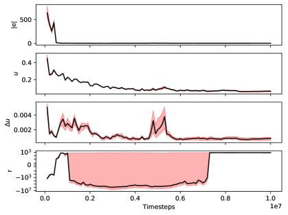
Figure 5$\cdot$16: PPO training validation.

PID Baseline Evaluation

To provide a performance baseline for our simulation evaluation, we use the traditional PID control algorithm. However the PID attitude controller requires 9 static gains to be tuned specific for our new digital twin. To accomplish this task we implemented a tuning platform using GymFCv2. This architecture is displayed in Fig. 5$\cdot$17. We will now discuss the user provided modules.

Control algorithm and tuner. We use the open source Ivmech PID Controller[pid, 2019] for the implementation of our attitude PID controller, for each of the three axis. As we have previously discussed in Section 2.3, the collective output of the three PID controllers, must be mixed together to form the control signal. We ported over the mixing implementation from Betaflight [bet, 2018] and with a little glue code to create our PID controller. To tune the PID controller, we use the classical Ziegler-Nichols method [Ziegler and Nichols, 1942].

Environment Interface We create an environment interface to provide command generation, and transformation functions of the aircraft state. To support tuning using the Ziegler-Nichols method, at $t=0$, we issue a command that is held for the entire duration of the simulation to obtain the step response from the controller. The environment can be provided with a specific setpoint to allow each axis to be tuned independently, or if absent, defaults to randomly sampling a setpoint so the performance can be randomly evaluated. The environment interface also transforms the aircraft state, into the angular velocity error which is requires as input to the PID controller.

Using the GymFCv2 PID tuning platform, we obtained the following gains for each axis of rotation: $K_{\phi}=[2.4,33.24,0.033]$, $K_{\theta}=[4.2,64.33,0.059]$, $K_{\psi}=[2,5,0]$, where $K_{\text{axis}}=[K_{P},K_{I},K_{D}]$ for each proportional, integrative, and derivative gains, respectively.

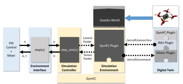
Figure 5$\cdot$17: Implementation of GymFCv2 for PID control tuning and SITL testing.

5.5.2 Simulation Evaluation

In this section we evaluate the neuro-flight controllers performance in simulation, and compare it to the previously tuned PID controller. We evaluated both controllers against 100 never before seen command inputs, using the episode environment (pulse control input) used during training of the NN-based controller. The average metrics are reported in Table 5.6 for the NN-based controller, while the PID controller metrics are reported in Table 5.7. Overall, results are consistent from our previous findings. The NN-based controller trained via PPO outperforms the PID controller in all of our error metrics. We additionally calculated the average control output produced by the controller, as well as the average absolute change in the control output. These values are also associated with their error, falling within a 95% confidence interval. For the NN controller, the average control output and change in output was $\overline{u}=$$0.12\pm 0.01$, and $\overline{|\Delta u|}=$$0.02\pm 0.01$ respectively. While for the PID controller, the average control output and change in output was $\overline{u}=$$0.03\pm 0.019$ and $\overline{|\Delta u|}=$$0.04\pm 0.02$ respectively. Although the PID controller uses less effort, for the first time in this work, we have been able to synthesize a controller that results in less change to the control output, and in effect, less oscillations, than that produced by a PID controller.

	NN Controller (PPO)
Metric	Roll ($\phi$)	Pitch($\theta$)	Yaw ($\psi$)	Average
MAE	3	2	2	2
MSE	148	135	66	117
IAE	3,311	2,235	2,075	2,541
ISE	148,804	135,805	66,807	117,138
ITAE	6,233	4,033	3,435	4,567
ITSE	237,168	211,846	95,983	181,666

Table 5.6: Simulation validation of performance metrics of NN controller trained with policy using digital twin. Metrics are reported for each individual axis, along with the average. Lower values are better.

	PID Controller
Metric	Roll ($\phi$)	Pitch($\theta$)	Yaw ($\psi$)	Average
MAE	4	4	3	4
MSE	414	492	199	368
IAE	4,773	4,941	3,829	4,514
ISE	414,216	493,033	199,662	368,970
ITAE	7,680	7,937	6,574	7,397
ITSE	608,092	712,863	300,222	540,392

Table 5.7: Simulation validation of performance metrics of PID controller trained with policy using digital twin. Metrics are reported for each individual axis, along with the average. Lower values are better.

We visually compare the performance between the PPO controller and the PID controller in Fig. 5$\cdot$18. In this example, the PID controller suffers significant overshoot in the yaw axis. With the exception of minor overshoot on the roll axis, the PPO controller tracks the setpoint quite well. We sample another episode and zoom in on the step response to the command in Fig. 5$\cdot$19. Here we can more clearly compare the control signals between the two controllers. In this figure, the legend is shared between the last two subplots which correspond to the control signal and motor RPM respectively. The control signals generated by the two controllers are very similar and follow similar responses. In the RPM plot, we can see the affect each control signal has on each motor velocity.

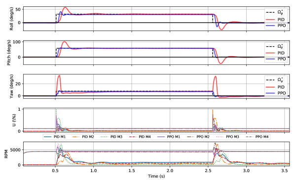
Figure 5$\cdot$18: Step response comparison between PPO-based flight controller, and PID flight controller.

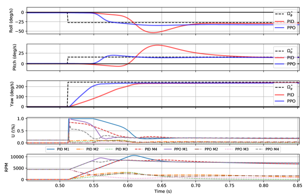
Figure 5$\cdot$19: Zoomed in comparison between PPO-based flight controller, and PID flight controller.

Flight envelope. In the following experiment, we wish to characterize the flight envelope of the two controllers. More specifically we would like to compare the operating regions of each controller, in regards to how well the controller can maintain a desired angular velocity.

To perform this measurement, we used the step input environment created for tuning the PID controller to randomly sample an angular velocity from a Gaussian distributions with $\mu=0$ and $\sigma=300$. For each controller we evaluate 1,000 different setpoints. For each trial, the mean absolute error (MAE) is calculated. We then created a 3D scatter plot, where each point is a setpoint, and its color corresponds to the MAE. Results for the PID controller and NN controller are displayed in Fig. 5$\cdot$20 and Fig. 5$\cdot$21 respectively. Looking closely at the scale of the color bar, we can see that the NN controller experiences almost three times less error in the evaluation region. To measure stability, we counted the number of times each controller was able to remain in a 10% error band, in relation to the setpoint, after 500ms have lapsed. The NN controller was able to stay within the error band, 72% of the time, compared to PID controller only doing so 16% of the time. We speculated the poor performance of the PID controller could be due to the slower rise time, or overshoot. We increased the time before we started measuring the error band till after 750ms which only increased the PID controller to 29%, however this also increased the NN to 76%. Manually inspecting the step response it became clear that once the set points diverged greatly from its tuning region, its became very unstable with significant oscillations. On the other hand, the NN controller was able to maintain stability upwards to angular velocities exceeding 1,000 degrees per second. These results showcase the robustness of the NN controller, and the expanded flight envelope in comparison to PID control.

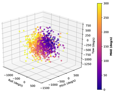
Figure 5$\cdot$20: Flight envelope of PID flight controller.

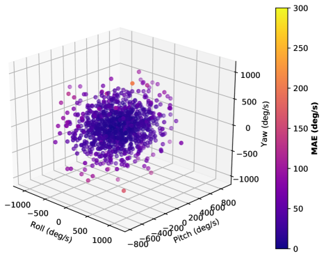
Figure 5$\cdot$21: Flight envelope of neuro-flight controller.

5.5.3 Neuroflight Flight Evaluations

In this section we perform real flight evaluation of the NN policy. Before conducting these test flights, we compile the policy into the Neuroflight firmware and flash our flight controller using the Neuroflight toolchain described in Section 4.4.

We conducted a total of 7 test flights executing a variety of basic and advanced flight maneuvers while logging the angular velocity reported by the gyro, the desired setpoint, and the motor control signals. All FPV videos of the test flights can be viewed at [Koch, 2018c]. The pilot reported precise and smooth handling. The FPV videos do not show any signs of oscillations of other issues. Furthermore the pilot did not experience the drifting issues that were reported in the policy trained with GymFCv1.5. Fig. 5$\cdot$22 shows the performance of the NN controller tracking the desired setpoint during one of the real flights. The controller is able to track the pitch axis remarkably well. To inspect the tracking more closely, we zoomed in on a roll being performed in Fig. 5$\cdot$23. With the exception of some minor oscillations in the pitch axis, the tracking of the setpoints is observed to be quite smooth.

Afterward the test flights were conducted, we analyzed the flight logs and generated the performance metrics reported in Table 5.8. These error metrics are an average across all test flights. Comparing these average errors to those from the controller trained with GymFCv1.5 in Table 4.7, we can see the drastic reduction in error through the use of training the policy using the digital twin. There is an 11 degrees per second decrease in the MAE as well as a significant drop is MSE indicating a decrease in large fluctuations in the error.

To measure the performance gap between the real world and simulation world, we took the desired angular velocities recorded during the test flights and played them back to the NN controller in the GymFCv2 simulation environment controlling the digital twin. The same error metrics were generated and are reported in Table 5.9. From this comparison we can see the reality gap has been greatly reduced. The average MAE for the simulation playback is 3 degrees per second which was also the same measured in the GymFCv1.5 environment. However we now only have a 2 degrees per second increase in MAE in the real world compared to 13 degrees per second previously measured when not using the digital twin (Table 4.7).

One important observation we made during the test flights was the immense heat being generated by the motors. This is usually a sign of rapid switching of the ESC. To prevent motor damage, we would allow the motors to cool between test flights. To quantify the switching in the control signals, we calculated the average absolute change in the control output ($\overline{|\Delta u|}$) to be $0.01\pm 5.5e-5$ in the real world, and $0.08\pm 2e-4$ in the simulation world.

The increase in the control signal output is problematic and confirmed our suspicions while in the field conducting test flights. Further experimental tests need to be conducted to validate whether the heat generated by the control signal oscillations are significant enough to cause damage to the motor wires and permanent magnets. Visually we can confirm the aggressive oscillations in Fig. 5$\cdot$23 of one of the test flights. What is most surprising is the significant gap in the performance between the oscillations in simulation verse the real world. Although we found the reward and environment described in Section 5.4 to train policies to transfer well to the real world, we experimented with dozens of other policies, each of which contained such severe visual oscillations, the test flights had to be abandoned. Through our experience, minimizing the control signal oscillations has been the greatest challenge.

Nevertheless, the accuracy of the NN controller in the real world, when trained using the digital twin, demonstrates remarkable tracking performance. We have established a solid foundation for synthesizing accurate controllers which can now be used to develop controllers with advanced control goals.

	NN Controller (PPO)
Metric	Roll ($\phi$)	Pitch($\theta$)	Yaw ($\psi$)	Average
MAE	6	5	3	5
MSE	136	64	53	84
IAE	4,438	3,846	2,748	3,677
ISE	96,779	46,009	37,865	60,218
ITAE	171,530	145,893	103,179	140,201
ITSE	3,952,545	1,847,723	1,866,962	2,555,743

Table 5.8: Average error metrics of the NN controller from flights in the real world trained with the digital twin. Metrics are reported for each individual axis, along with the average. Lower values are better.

	NN Controller (PPO)
Metric	Roll ($\phi$)	Pitch($\theta$)	Yaw ($\psi$)	Average
MAE	3	3	4	3
MSE	35	20	26	27
IAE	3,879	3,337	4,091	3,769
ISE	35,144	20,928	26,893	27,655
ITAE	101,586	86,477	106,814	98,293
ITSE	955,123	554,219	708,319	739,220

Table 5.9: Error metrics of simulation playback NN controller trained with policy using digital twin. Metrics are reported for each individual axis, along with the average. Lower values are better.

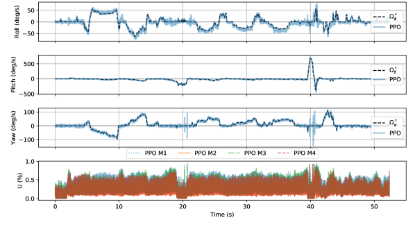
Figure 5$\cdot$22: Flight test for neuro-flight controller synthesized with digital twin.

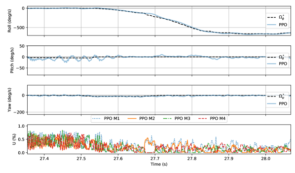
Figure 5$\cdot$23: Zoomed in portion of a roll being executed.

5.5.4 Discussion

Throughout this research, one of the most difficult challenges has been managing the NN control signal oscillations. Through discussions with other researchers, this appears to be a challenge, not only for flight control, but neuro-control in general. Reducing oscillations has been discussed briefly in some of the literature. For helicopter RL-based navigation controllers, [Bagnell and Schneider, 2001] added a low pass digital filter to the control signal outputs, while in [Kim et al., 2004], a penalty based on the quadratic sum of actions is used to promote smooth and small changes to the output.

It is perplexing that the only other work that discusses concerns with output oscillations for quadcopter control is in [Molchanov et al., 2019]. In this work they found removing the gyro low pass filter in the CrazyFlie firmware, decrease delay, while also decreasing physical oscillations. However we did not find this to help. This is most likely due to us sampling the gryo at a considerably faster speed. In this work we sample the gyro at 4kHz and execute our control loop at 1kHz, while work in [Molchanov et al., 2019] executes their control loop at 500Hz. This work also reports the highest frequency found in the control signal output, however without any relationship to performance (i.e., causes visual oscillations, increases motor temperature, etc.) these metrics are not meaningful as different propeller propulsion systems will be affected differently by the control signal.

Other work related to NN-based flight control [Hwangbo et al., 2017, Palossi et al., 2019] have not reported any details relating to the control signals generated by their neuro-controller. Thus the questions arise, do the control signals oscillate more than traditional control methods, such as PID? If not, what is different about their approach such that this is not a concern? In [Hwangbo et al., 2017] the authors combine the output of a PD controller with the NN, for attitude control, during training in order to stabilize the learning process. The authors mention it does not aid the controller after the training process however it is unclear if it is removed from the controller when transferred to hardware. If it is removed, this work does not discuss how the controller compensates for the absence of the PD controller output. One possible reason high oscillations are not as prominent could be due to the differences in control goals. Our work is concerned with low level control while the previously mentioned work is related to guidance and navigation tasks. Perhaps position estimation provided by motion capture systems and video results in decreased control signal oscillations. If this can be verified it would be interesting future work to explore.

5.6 Related Work

In this section we will review simulators used for flight control testing, the aircraft models they provide and motor models they use. Additionally we will review work related to UAV propulsion system modelling.

5.6.1 Flight Simulators and Aircraft Models

The Gazebo simulator provides an Iris quadcopter, and Zephr fixed wing UAV aircraft model. To achieve flight, an aerodynamic plugin is provided. For a multicopter, the aerodynamic plugin calculates the lift for each blade and motor response from a PID controller.

RotorS [Furrer et al., 2016] is a micro air vehicle (MAV) Gazebo simulator framework for software in the loop testing of flight control systems with a focus in navigation and guidance. The framework is tightly integrated with the Robotics Operating System (ROS) and includes a number of multirotor models such as the AscTec Hummingbird, the AscTec Pelican, or the AscTec Firefly. Their documentation briefly describes how to assemble your own MAV into their simulator however this does not describe methods for motor modelling. Additionally they acknowledge challenges transferring to a real MAV and share the same goals as this work to reduce effort transferring to real hardware however this also requires the target real aircraft to support ROS as well.

The PX4 project has extracted the motor models and dynamics from RotorS to create a new project that is independent of ROS for SITL and HITL testing [px4, 2019]. Unfortunately there does not exist any documentation for deriving your own motor models.

AirSim [Shah et al., 2018] has similar goals to RotorS with a focus in computer vision. To create realistic environments, this simulator uses the Unreal engine which is difficult to achieve in Gazebo. The Unreal engine uses PhysX [phy, 2019] as the physics engine backend which supports both generalized and maximal coordinate solvers.

Both RotoS and AirSim derive the motor forces and torques in a similar fashion using element blade element theory [McCormick, 1995] and model motor response using first order filters. This method derives the force and torques from the entire motor and propeller pair rather than Gazebo’s aerodynamic which calculates these forces from the individual blades.

Our work shares many of the same ambitions as the previous work primarily in regards of providing seamless transfer to hardware. However previous work is primarily focused in higher level tasks while GymFC’s primary goal is to provide a tuning framework with a focus in low level attitude control.

5.6.2 Propeller Propulsion System Data

A propeller database published by University of Illinois Urbana-Champaign contains wind tunnel measurements for over 200 small-scale propellers [Brandt et al., 2015]. The database contains the advance ratios, thrust and torque coefficients. Details of the experimental methodology and the test stand are presented in [Deters et al., 2014]. Follow up work [Deters et al., 2017] performed static propeller testing for four popular quadcopters including the 3D Robotics Solo and DJI Phantom 3. Thrust and power coefficients are also reported.

In [Gong et al., 2018] a study of propeller propulsion systems, including the ESC was conducted. Models were also developed for the ESC. The model was derived by fitting the efficiency data to a bi-linear equation as a function of the throttle and current.

Unfortunately of the previously discussed work, time behavior of the propulsion system is not reported thus a motor response model can be not obtained.

A large database of static propeller propulsion system performance data, commonly found on multicopters has been published by MiniquadTestBench [min, 2018]. Thrust, torque, power and motor velocity have been recorded for a number of different control inputs. Although thrust and power coefficients are not provided, one could derive these values from the raw data. Given the raw data one is also able to measure the motor response.

5.7 Conclusion and Future Work

In this work we present a universal tuning framework, GymFCv2, as a means to synthesizing neuro-flight controllers unique to their digital twin aircraft. We introduce our methodology for creating a digital twin and demonstrate the approach producing a digital twin for the NF1. Using our digital twin we analyze its stability in the Gazebo simulator using the default physics engine ODE and compare these results to DART.

We further showcase the flexibility of the GymFCv2 framework through the implementation of a dynamometer for validating motor model thrust, torque and velocity performance, as well as a platform for PID tuning. Evaluating our synthesized neuro-flight controller in simulation, we find this class of controllers has a larger flight envelope than a classical PID controller. Our real world flight evaluations provide convincing evidence training using the digital twin reduced the reality gap. Nonetheless, the controller experienced high frequency motor output oscillations that must be addressed in future work. In summary, our future work consists of making improvements to the digital twin, and addressing control signal oscillations.

We have identified three potential sources of error in the aircraft model that need further attention in future work.

1. Moments of inertia. In this work we compute the moments of inertia using the measured mass of each individual aircraft part and the moments of inertia matrix measured from each mesh model. However as we previously discussed in Section 5.2.1 these methods assume a uniform mass distribution of the object. In future work we will investigate methods for validating the accuracy of our approach through experimental real world measurements. Possible approaches may consist of building a torsional pendulum and an apparatus for the aircraft body to derive the inertia measurements.

2. Motor model. To model motor dynamics we have used the PX4 motor models as a foundation which embodies established models from element blade theory. However as we have seen in our experimental measurements, the torque and thrust coefficients greatly vary in relation to the motor RPM. Thus using static thrust and torque coefficient will introduce errors. Based on these observations in the future we plan to develop more accurate models and investigate using NN to train an inverse plant model of the motor model.

3. Aircraft attitude. The challenge of developing the digital twin is being able to model the individual components and then compose them such that the resulting model is accurate. In regards to the motor performance, we were able to validate the thrust, torque and rotor velocity models in simulation. In the future we plan to validate the angular velocity of the aircraft in the real world. This will require the developed of an apparatus to fix the aircraft along each axis with sensors to measure the angular velocity of the aircraft body. From this data we can calculate other forces acting upon the aircraft such as drag to further improve the accuracy of the simulation.

In regards to addressing oscillations in the control signal outputs experienced in the real world, we plan to take the following approaches.

1. NN state and architectures The ultimate goal is to develop a neuro-controller which can make its decisions based on the complete internal state of the aircraft. Thus we must work towards integrating addition sensors as input, while still maintaining a high level of performance. For one, we would like to perform experiments to identify if any correlation exists between the motor temperate and the ESC temperature. If so, we are able to access the ESC temperate through ESC telemetry which can aid in building policies to prevent the aircraft getting into a state that could cause damage, for example shorting the motor wires.

2. Domain randomization In the future we plan to integrating additional dynamics and forces, such wind, gravity, and other generic force acting upon the aircraft body. In this work we emulated gyro noise that was modelled from empirical data. However in future work we plan to investigate other domain randomization techniques such action delays and noise to the set point.

Work and results outlined in this chapter have helped progress the state-in-the-art in intelligent flight control, bringing us one step closer to these controllers being practical to be adopted in the real world.

Chapter 6 Conclusions

The rapid advances in machine learning, big data, material sciences and manufacturing will transform the aviation industry as we know it. The aircraft of the future will be self-aware providing remarkable levels of performance, safety and reliability. This will be in part due to advanced flight control systems, providing the abilities to learn, plan and adapt. For example, the aircraft will be able to learn its current flight envelope to determine what its current capabilities are. Furthermore, the aircraft will be able to plan, in real-time, for potential future system failures and mitigate them from occurring before they happen. Lastly, the aircraft will be able to adapt to changes, such as shifts in payload. To support these advanced control goals we require a new generation of intelligent control systems that will be capable of providing high order executive functions. To that end, this dissertation makes the following contributions.

6.1 Summary of Contributions

This dissertation investigates using the digital twinning paradigm for synthesizing NN based flight control systems. The resulting flight controller is unique to the digital twin, providing optimal control for the specific aircraft digital twin. Using NNs, these controllers have the fundamental building blocks to support our future advanced control goals that are out of reach of traditional control methods. This work has established a foundation for these next generation flight control systems, by developing software to synthesize stable, precise and accurate NN-based attitude controllers. Specifically, we developed a full solution stack for synthesizing NN-based flight controllers via RL. This solution stack consists of a universal tuning framework called GymFC, a digital twin development methodology, and a NN supported flight control firmware named Neuroflight. In summary this dissertation makes the following contributions in the study of intelligent flight control systems.

Tuning framework and training environment. In this work we introduce GymFC, an open source universal flight control tuning framework. We implement an RL training environment using GymFC and benchmark a number of state-of-the-art RL algorithms, in simulation for quadcopter attitude control, including DDPG, TRPO and PPO. We find PPO to out perform all other RL algorithms, as well as traditional PID control.

We introduce the reward function used to synthesize attitude flight controllers via RL which achieves remarkable accuracy in the real world. We further showcase the modular design of the GymFC framework implementing a virtual dynamometer for motor modelling and an environment for PID control tuning. The GymFC architecture provides a platform for researchers to develop tools and environments to aid in developing next generation flight control. Furthermore, GymFC opens up new possibilities for performing SITL and HITL sensitivity analysis of various environment, controller and aircraft parameters to aid in controller and aircraft design.

Digital twin development. To reduce the reality gap we have proposed our methodology for creating a digital twin of a multicopter. This included the creation of the aircraft rigid bodies, and the construction of a dynamometer to obtain measurements for deriving motor models. We have developed motor response models to increase realism of the motor dynamics. Additionally, we have published software to perform a stability analysis of the digital twin in simulation. Our evaluations show the digital twin has almost completely eliminated the reality gap in terms of angular velocity error.

Flight control firmware. This dissertation introduced Neuroflight, the world’s first open source NN supported flight control firmware. We have proposed our toolchain for deploying a trained NN policy to highly resource constrained off-the-shelf microcontrollers. Our timing analysis shows the NN controller can execute faster than 2kHz allowing for faster digital ESC protocols to be utilized to support high precision flight. Our real world flight evaluations demonstrate the NN policies provide stable, accurate flight and are capable of performing aerobatic maneuvers.

6.2 Open Challenges and Future Work

The work proposed in this dissertation establishes a foundation for next generation flight control systems however this is just the first stepping stone and a number of opportunities lie ahead for future work.

1. Simulation improvements. GymFC is able to train attitude controllers independent of navigation tasks through our approach of fixing the aircraft about its center of thrust to the simulation world. Although autonomous flight control is currently more prominent in literature than low level attitude control, manual override and be necessary for these control systems to be adopted in the real world. Unfortunately the majority of work related to autonomous flight do not address these issues. Our training strategy allows for the agent to learn the mapping of the desired angular velocity setpoint to the corresponding motor control signal however there are side affects that we have previously discussed in Section 4.3.2 such as the agent using more power than needed. We are able to compensated for this undesired behavior through the reward functions however this is not ideal as increasing reward complexity can affect tracking accuracy.

   The quadcopters we have trained in this work are agile racing drones, however one must be careful with command generation if the aircraft is not balanced. Multicopters where the center of mass does not equal the center of thrust, for example because of a gimbal, may not have the capability to perform full rotations in the simulation environment. For these type of aircraft one must make sure they will stay within their flight envelope, which will result in additional logic for command generation during training.

   To further increase realism of the environment additional environment dynamics need to be modelled such as gravity, wind, aerodynamic affects of the aircraft and other external disturbances acting upon the body during flight.

2. Digital twin development. The modular design of the GymFC framework opens up a number of possibilities for increasing the fidelity of the digital twin. This could include the integration of power models to simulate discharging of a battery, and modelling material stress-strain analysis. Furthermore, in Chapter 5.2 we identified and discussed a number of errors in the motor model, such as using a static torque and thrust coefficient which does not accurately model the nonlinear motor dynamics that are exaggerated for smaller multicopters such as our racing drone.

   This work has been scoped to synthesizing flight controllers offline and as a result we have not investigated methods for synchronizing the digital twin with the real aircraft after it is deployed in the real world. To achieve the true potential of the digital twin, future work must develop methods for updating the digital twin with data obtained from the real aircraft so the controller, in the virtual environment, can continually be improved. Essentially we need to create an inverse plant of the aircraft however current modelling depends on the thrust and torque of each motor which can be difficult to obtain during flight.

3. Continuous learning. Our current approach trains NNs exclusively using offline learning. However, in order to reduce the performance gap between the simulated and real world we expect that a hybrid architecture involving online incremental learning will be necessary. Online learning will allow the aircraft to adapt, in real-time, and compensate for any modelling errors that existed during offline training. This presents interesting challenges for designing architectures to hot-swap the NN weights. If we recall from Chapter 4 when the flight controller is trained offline, the resulting NN graph is “frozen” and AOT-compiled to execute on the quadcopters onboard controller. The compiled NN is a mix of arithmetic operations and hard-coded network weights and is treated just as any other function. For resource constrained environments loading large networks into memory may not be an option. Thus we will need to develop new software, and hardware architectures that can support this functionality.

   Online learning will be complimentary to training on the digital twin. The digital twin can utilize the power of the cloud to perform heavier computation than the aircraft’s onboard computer. For example, the digital twin can be used to run through multiple different scenarios, and forecast system failures before they occur.

4. NN architecture. Several performance benefits can be realized from an optimal network architecture for flight control including improved accuracy and faster execution. An extensive survey needs to be conducted investing the pros and cons of various architectures.

   Long short-term memory (LSTM) networks may help with time varying dynamics such as the motor response. Alternative distributions such as the beta function which is naturally bounded [Chou et al., 2017] may help with motor oscillation issues. Furthermore the use of the rectified linear unit (ReLU) activation functions may reduce the execution time of the NN due to it being more computationally efficient than the hyperbolic tangent function.

   Moving forward it will be important to develop modular networks. The current research direction of RL based flight controllers for navigation are do not allow for manual flight [Hwangbo et al., 2017, Palossi et al., 2019]. For these controllers to be deployed in the real world there must be a way to manually pilot the aircraft for maintenance and management purposes. Using hierarchical network structures could be beneficial in creating modular neuro-flight controllers.

An exciting future lies ahead for developing next generation aircraft and their corresponding flight control systems. As embedded computing platforms continue to reduce in size, it will allow for revolutionary advancements in flight control, supporting sophisticated control goals such as the ability to learn, plan and adapt. The work presented in this thesis has provided a foundation for the community to build upon, using our solution stack to explore the full potential of NN-based flight control systems.

Education

• Boston University Boston, MA
  PhD in Computer Science Sept. 2014 - Sept. 2019
  Thesis title: Flight Controller Synthesis via Deep Reinforcement Learning
  GPA: 3.7/4.0

• Stevens Institute of Technology Hoboken, NJ
  M.S. in Computer Engineering Jan. 2012 - Dec. 2013
  Thesis title: A framework for assisting learners by incorporating knowledge to aid in predicting nerve guidance conduit performance
  GPA: 3.8/4.0

• University of Rhode Island Kingston, RI
  B.S. in Computer Engineering, Minor in Mathematics Sept. 2003 - May 2008
  GPA: 3.2/4.0

Research Experience

• Boston University Boston, MA
  Research Assistant Jan. 2017 - Present

  • Developing next generation flight control systems through the use of machine learning including the worlds first open-source neural network powered flight control firmware, Neuroflight.

  • Conducted research in wide area of cyber security including static and dynamic malware analysis, vulnerability analysis, cyber defense and attacks and mobile security.

• MIT Lincoln Laboratory Lexington, MA
  Cyber Security Research Intern Jan. 2016 - June 2016

  • Developed novel SDN attack called Persona Hijacking which has been published in USENIX Security Symposium.

• Stevens Institute of Technology Hoboken, NJ
  Research Assistant Jan. 2012 - Dec. 2013

  • Worked on multi-discipline team consisting of biomedical and computer engineers to advance nerve guidance conduit performance.

  • Developed novel machine learning algorithms to predict nerve guidance conduit performance.

Teaching Experience

• Boston University Boston, MA
  Teaching Fellow Fall 2017, Spring 2019

  • Designed lesson plans, taught discussion sections, developed written and programming assignments for class Fundamentals of Computing Systems.

• Internal Drive Tech Camps Princeton, NJ
  Programming Instructor June 2016 - Aug. 2018

  • Created lesson plans for wide range of skill levels including object oriented fundamentals, polymorphism, exception handling and third-party library integration.

  • Emphasized lessons on coding style and best practices not taught and enforced in academia.

  • Advised students through final projects ranging from web crawlers to video games.

• Stevens Institute of Technology Hoboken, NJ
  Teachers Assistant Jan. 2012 - Dec. 2013

  • Grader for graduate class CPE-555 Real-Time and Embedded Systems and undergraduate class EE-250 Mathematics for Electrical Engineers.

Additional Experience

• Boston Drone Racing Boston, MA
  Founder Jan. 2017 - Present

  • Created website and designed logo. Established communication channels. Manage social media networks.

  • Secured funding for racing track and supplies.

  • Organize weekly races and monthly hack nights.

• Capsules, LLC Madison, CT
  Co-Founder/CEO June 2013 - Aug. 2014

  • Managed team to create a geo-location based augmented reality mobile app.

  • Lead mobile developer responsible for overall architecture, design and implementation.

• Sikorsky Aircraft (subcontracted through AIS Consulting and Sila SG) Shelton, CT
  Software Engineer Jun. 2006 - Jan. 2012

  • Lead software engineer on seven software applications for the Sikorsky CH-53K Aircraft’s Integrated Support System (ISS).

  • Designed and implemented continuous integration environment.

  • Responsible for integration between third-party vendors.

• CT Hackerspace Watertown, CT
  Co-founder/Chairman Aug. 2010 - Aug. 2011

  • Established organization through the development of bylaws, identity, physical and web presence.

  • Ran monthly board meetings to facilitate in the growth and direction of the hackerspace.

Select Publications

• Neuroflight: Next Generation Flight Control Firmware William Koch, Renato Mancuso, and Azer Bestavros, In submission 2019

• Reinforcement Learning for UAV Attitude Control William Koch, Renato Mancuso, Richard West, and Azer Bestavros, ACM Transactions on Cyber-Physical Systems 2019

• S3B: Software-Defined Secure Server Bindings William Koch, and Azer Bestavros, IEEE International Conference on Distributed Computing Systems (ICDCS) 2018

• Semi-automated discovery of server-based information oversharing vulnerabilities in Android applications William Koch, Abdelberi Chaabane, Manuel Egele, William Robertson, and Engin Kirda, ACM SIGSOFT International Symposium on Software Testing and Analysis 2017

• PayBreak: defense against cryptographic ransomware. Eugene Kolodenker, William Koch, Gianluca Stringhini, and Manuel Egele, ACM on Asia Conference on Computer and Communications Security 2017

• Identifier Binding Attacks and Defenses in Software-Defined Networks Samuel Jero, William Koch, Richard Skowyra, Hamed Okhravi, Cristina Nita-Rotaru, and David Bigelow, USENIX Security Symposium 2017

• Markov modeling of moving target defense games Hoda Maleki, Saeed Valizadeh, William Koch, Azer Bestavros, and Marten van Dijk, In Proceedings of the 2016 ACM Workshop on Moving Target Defense 2016

• Provide: Hiding from automated network scans with proofs of identity William Koch, and Azer Bestavros, IEEE Workshop on Hot Topics in Web Systems and Technologies (HotWeb) 2016

Projects

• Neuroflight Neuroflight is the first open-source neuro-flight controller software (firmware) for remotely piloting multi-rotors and fixed wing aircraft. Neuroflight’s primary focus is to provide optimal flight performance.
  https://github.com/wil3/neuroflight

• GymFC GymFC is an OpenAI Gym environment designed for synthesizing intelligent flight control systems using reinforcement learning. This environment is meant to serve as a tool for researchers to benchmark controllers to progress the state-of-the art of intelligent flight control.
  https://github.com/wil3/gymfc

Bibliography

- [lea, 2015] (2015). Brushless motor constant explained. http://learningrc.com/motor-kv/. Accessed: 2018-12-07.
- [ard, 2018] (2018). ArduPilot. http://ardupilot.org/. Accessed: 2018-03-13.
- [baz, 2018] (2018). Bazel - a fast, scalable, multi-language and extensible build system. https://bazel.build/. Accessed: 2018-11-25.
- [bet, 2018] (2018). BetaFlight. https://github.com/betaflight/betaflight. Accessed: 2017-10-18.
- [cle, 2018] (2018). CleanFlight. Accessed: 2018-11-25.
- [gzb, 2018] (2018). gzserver doesn’t close disconnected sockets. https://bitbucket.org/osrf/gazebo/issues/2397/gzserver-doesnt-close-disconnected-sockets. Accessed: 2018-03-13.
- [iri, 2018] (2018). Iris Quadcopter. http://www.arducopter.co.uk/iris-quadcopter-uav.html. Accessed: 2018-03-28.
- [min, 2018] (2018). Motor Data Explorer. https://www.miniquadtestbench.com/motor-explorer.html. Accessed: 2018-11-25.
- [rot, 2018] (2018). NF1: Neuroflight Test Aircraft 1. https://rotorbuilds.com/build/15163. Accessed: 2018-11-25.
- [pro, 2018] (2018). Protocol Buffers. https://developers.google.com/protocol-buffers/. Accessed: 2018-03-13.
- [STM, 2018] (2018). STM32F745VG. https://www.st.com/en/microcontrollers/stm32f745vg.html. Accessed: 2018-11-25.
- [ten, 2018] (2018). Tensorflow:An Open Source Machine Learning Framework for Everyone. https://github.com/tensorflow/tensorflow/. Accessed: 2018-11-25.
- [erl, 2019] (2019). Erle-copter. http://docs.erlerobotics.com/erle_robots/erle_copter. Accessed: 2019-07-26.
- [fre, 2019] (2019). FreeCAD. https://www.freecadweb.org/. Accessed June 17, 2019.
- [px4, 2019] (2019). Gazebo Sim Plugin. https://github.com/PX4/sitl_gazebo. Accessed June 17, 2019.
- [ine, 2019] (2019). Inertial parameters of triangle meshes. http://gazebosim.org/tutorials?tut=inertia&cat=build_robot. Accessed June 17, 2019.
- [int, 2019] (2019). Intel Aero. https://click.intel.com/intel-aero-ready-to-fly-drone-2679.html. Accessed: 2019-07-26.
- [phy, 2019] (2019). PhysX. https://gameworksdocs.nvidia.com/PhysX/4.0/documentation/PhysXGuide/Manual/Introduction.html. Accessed: 2019-07-20.
- [pid, 2019] (2019). Python PID Controller. https://github.com/ivmech/ivPID. Accessed: 2019-07-26.
- [rcb, 2019] (2019). RCbenchmark. https://www.rcbenchmark.com/. Accessed June 17, 2019.
- [sdf, 2019] (2019). SDFormat. http://sdformat.org/. Accessed June 17, 2019.
- [Abbeel et al., 2007] Abbeel, P., Coates, A., Quigley, M., and Ng, A. Y. (2007). An application of reinforcement learning to aerobatic helicopter flight. In Advances in neural information processing systems, pages 1–8.
- [Abdulrahim et al., 2019] Abdulrahim, M., Bates, T., Nilson, T., Bloch, J., Nethery, D., and Smith, T. (2019). Defining flight envelope requirements and handling qualities criteria for first-person-view quadrotor racing. In AIAA Scitech 2019 Forum, page 0825.
- [Andrychowicz et al., 2018] Andrychowicz, M., Baker, B., Chociej, M., Jozefowicz, R., McGrew, B., Pachocki, J., Petron, A., Plappert, M., Powell, G., Ray, A., et al. (2018). Learning dexterous in-hand manipulation. arXiv preprint arXiv:1808.00177.
- [Åström and Wittenmark, 2013] Åström, K. J. and Wittenmark, B. (2013). Adaptive control. Courier Corporation.
- [Bagnell and Schneider, 2001] Bagnell, J. A. and Schneider, J. G. (2001). Autonomous helicopter control using reinforcement learning policy search methods. In Robotics and Automation, 2001. Proceedings 2001 ICRA. IEEE International Conference on, volume 2, pages 1615–1620. IEEE.
- [Black et al., 2014] Black, W. S., Haghi, P., and Ariyur, K. B. (2014). Adaptive systems: History, techniques, problems, and perspectives. Systems, 2(4):606–660.
- [Blitzer et al., 2008] Blitzer, J., Crammer, K., Kulesza, A., Pereira, F., and Wortman, J. (2008). Learning bounds for domain adaptation. In Advances in neural information processing systems, pages 129–136.
- [Bobtsov et al., 2016] Bobtsov, A., Guirik, A., Budko, M., and Budko, M. (2016). Hybrid parallel neuro-controller for multirotor unmanned aerial vehicle. In Ultra Modern Telecommunications and Control Systems and Workshops (ICUMT), 2016 8th International Congress on, pages 1–4. IEEE.
- [Bouabdallah et al., 2004] Bouabdallah, S., Murrieri, P., and Siegwart, R. (2004). Design and control of an indoor micro quadrotor. In Robotics and Automation, 2004. Proceedings. ICRA’04. 2004 IEEE International Conference on, volume 5, pages 4393–4398. IEEE.
- [Brandt et al., 2015] Brandt, J. B., Deters, R. W., Ananda, G. K., and Selig, M. S. (2015). https://m-selig.ae.illinois.edu/props/propDB.html. Accessed: 2019-07-20.
- [Brockman et al., 2016] Brockman, G., Cheung, V., Pettersson, L., Schneider, J., Schulman, J., Tang, J., and Zaremba, W. (2016). OpenAI Gym. arXiv preprint arXiv:1606.01540.
- [Brooks, 1992] Brooks, R. A. (1992). Artificial life and real robots. In Proceedings of the First European Conference on artificial life, pages 3–10.
- [Cheng et al., 2018] Cheng, Z., West, R., and Einstein, C. (2018). End-to-end analysis and design of a drone flight controller. IEEE Transactions on Computer-Aided Design of Integrated Circuits and Systems, 37(11):2404–2415.
- [Chou et al., 2017] Chou, P.-W., Maturana, D., and Scherer, S. (2017). Improving stochastic policy gradients in continuous control with deep reinforcement learning using the beta distribution. In Proceedings of the 34th International Conference on Machine Learning-Volume 70, pages 834–843. JMLR. org.
- [Cignoni et al., 2008] Cignoni, P., Callieri, M., Corsini, M., Dellepiane, M., Ganovelli, F., and Ranzuglia, G. (2008). Meshlab: an open-source mesh processing tool. In Eurographics Italian chapter conference, volume 2008, pages 129–136.
- [Coumans, 2014] Coumans, E. (2014). Exploring mlcp solvers and featherstone. In Game Developers Conf, pages 17–21.
- [Coumans, 2015] Coumans, E. (2015). Bullet physics simulation. In ACM SIGGRAPH 2015 Courses, SIGGRAPH ’15, New York, NY, USA. ACM.
- [Cybenko, 1989] Cybenko, G. (1989). Approximation by superpositions of a sigmoidal function. Mathematics of control, signals and systems, 2(4):303–314.
- [Deters et al., 2014] Deters, R. W., Ananda Krishnan, G. K., and Selig, M. S. (2014). Reynolds number effects on the performance of small-scale propellers. In 32nd AIAA applied aerodynamics conference, page 2151.
- [Deters et al., 2017] Deters, R. W., Kleinke, S., and Selig, M. S. (2017). Static testing of propulsion elements for small multirotor unmanned aerial vehicles. In 35th AIAA Applied Aerodynamics Conference, page 3743.
- [Dewey, 2014] Dewey, D. (2014). Reinforcement learning and the reward engineering principle. In 2014 AAAI Spring Symposium Series.
- [Dhariwal et al., 2017] Dhariwal, P., Hesse, C., Klimov, O., Nichol, A., Plappert, M., Radford, A., Schulman, J., Sidor, S., and Wu, Y. (2017). Openai baselines. https://github.com/openai/baselines.
- [Dierks and Jagannathan, 2010] Dierks, T. and Jagannathan, S. (2010). Output feedback control of a quadrotor uav using neural networks. IEEE transactions on neural networks, 21(1):50–66.
- [dos Santos et al., 2012] dos Santos, S. R. B., Givigi, S. N., and Júnior, C. L. N. (2012). An experimental validation of reinforcement learning applied to the position control of uavs. In 2012 IEEE International Conference on Systems, Man, and Cybernetics (SMC), pages 2796–2802. IEEE.
- [Duan et al., 2016] Duan, Y., Chen, X., Houthooft, R., Schulman, J., and Abbeel, P. (2016). Benchmarking deep reinforcement learning for continuous control. In International Conference on Machine Learning, pages 1329–1338.
- [Ebeid et al., 2018] Ebeid, E., Skriver, M., Terkildsen, K. H., Jensen, K., and Schultz, U. P. (2018). A survey of open-source uav flight controllers and flight simulators. Microprocessors and Microsystems, 61:11–20.
- [Falkner et al., 2018] Falkner, S., Klein, A., and Hutter, F. (2018). Bohb: Robust and efficient hyperparameter optimization at scale. arXiv preprint arXiv:1807.01774.
- [Farha, 2016] Farha, F. (2016). Hovakimyan’s adaptive control to be tested on fighter jet. https://mechanical.illinois.edu/news/hovakimyans-adaptive-control-be-tested-fighter-jet. Accessed: 2019-07-18.
- [Fatan et al., 2013] Fatan, M., Sefidgari, B. L., and Barenji, A. V. (2013). An adaptive neuro pid for controlling the altitude of quadcopter robot. In Methods and models in automation and robotics (mmar), 2013 18th international conference on, pages 662–665. IEEE.
- [Furrer et al., 2016] Furrer, F., Burri, M., Achtelik, M., and Siegwart, R. (2016). Robot Operating System (ROS): The Complete Reference (Volume 1), chapter RotorS—A Modular Gazebo MAV Simulator Framework, pages 595–625. Springer International Publishing, Cham.
- [Gabor et al., 2016] Gabor, T., Belzner, L., Kiermeier, M., Beck, M. T., and Neitz, A. (2016). A simulation-based architecture for smart cyber-physical systems. In Autonomic Computing (ICAC), 2016 IEEE International Conference on, pages 374–379. IEEE.
- [Glaessgen and Stargel, 2012] Glaessgen, E. H. and Stargel, D. (2012). The digital twin paradigm for future nasa and us air force vehicles. In 53rd Struct. Dyn. Mater. Conf. Special Session: Digital Twin, Honolulu, HI, US, pages 1–14.
- [Gong et al., 2018] Gong, A., MacNeill, R., and Verstraete, D. (2018). Performance testing and modeling of a brushless dc motor, electronic speed controller and propeller for a small uav application. In 2018 Joint Propulsion Conference, page 4584.
- [Grieves, 2014] Grieves, M. (2014). Digital twin: Manufacturing–excellence through virtual factory replication (white paper). Michael Grieves (University of Michigan) LLC (http://innovate. fit. edu/plm/documents/doc_mgr/912/1411.0 _Digital_Twin_White_Paper_Dr_Grieves. pdf).
- [Hagan and Demuth, 1999] Hagan, M. T. and Demuth, H. B. (1999). Neural networks for control. In American Control Conference, 1999. Proceedings of the 1999, volume 3, pages 1642–1656. IEEE.
- [Hattem, 2019] Hattem, R. (2019). numpy-stl. https://numpy-stl.readthedocs.io/en/latest/. Accessed June 17, 2019.
- [Henderson et al., 2018] Henderson, P., Islam, R., Bachman, P., Pineau, J., Precup, D., and Meger, D. (2018). Deep reinforcement learning that matters. In Thirty-Second AAAI Conference on Artificial Intelligence.
- [Hill et al., 2018] Hill, A., Raffin, A., Traore, R., Dhariwal, P., Hesse, C., Klimov, O., Nichol, A., Plappert, M., Radford, A., Schulman, J., Sidor, S., and Wu, Y. (2018). Stable baselines. https://github.com/hill-a/stable-baselines.
- [Hovakimyan et al., 2011] Hovakimyan, N., Cao, C., Kharisov, E., Xargay, E., and Gregory, I. M. (2011). L1 adaptive control for safety-critical systems. IEEE Control Systems, 31(5):54–104.
- [Hunt et al., 1992] Hunt, K. J., Sbarbaro, D., Żbikowski, R., and Gawthrop, P. J. (1992). Neural networks for control systems—a survey. Automatica, 28(6):1083–1112.
- [Husbands and Harvey, 1992] Husbands, P. and Harvey, I. (1992). Evolution versus design: Controlling autonomous robots. In AI, Simulation and Planning in High Autonomy Systems, 1992. Integrating Perception, Planning and Action., Proceedings of the Third Annual Conference of, pages 139–146. IEEE.
- [Hwangbo et al., 2017] Hwangbo, J., Sa, I., Siegwart, R., and Hutter, M. (2017). Control of a quadrotor with reinforcement learning. IEEE Robotics and Automation Letters, 2(4):2096–2103.
- [Jakobi et al., 1995] Jakobi, N., Husbands, P., and Harvey, I. (1995). Noise and the reality gap: The use of simulation in evolutionary robotics. Advances in artificial life, pages 704–720.
- [Karpathy, 2018] Karpathy, A. (2018). Deep Reinforcement Learning: Pong from Pixels. Accessed: 2018-03-29.
- [Kim et al., 1993] Kim, B. S., Calise, A., and Kam, M. (1993). Nonlinear flight control using neural networks and feedback linearization. In Proceedings. The First IEEE Regional Conference on Aerospace Control Systems,, pages 176–181. IEEE.
- [Kim et al., 2004] Kim, H. J., Jordan, M. I., Sastry, S., and Ng, A. Y. (2004). Autonomous helicopter flight via reinforcement learning. In Advances in neural information processing systems, pages 799–806.
- [Koch, 2018a] Koch, W. (2018a). GymFC. https://github.com/wil3/gymfc.
- [Koch, 2018b] Koch, W. (2018b). Neuroflight Github Repository. https://github.com/wil3/neuroflight.
- [Koch, 2018c] Koch, W. (2018c). Neuroflight Project Page. https://wfk.io/neuroflight.
- [Koch, 2019a] Koch, W. (2019a). GymFC Aircraft Plugins. Accessed June 17, 2019.
- [Koch, 2019b] Koch, W. (2019b). Py3Gazebo: Python3 bindings for the Gazebo multi-robot simulator. https://github.com/wil3/py3gazebo. Accessed June 17, 2019.
- [Koch et al., 2019a] Koch, W., Mancuso, R., and Bestavros, A. (2019a). Neuroflight: Next generation flight control firmware. arXiv preprint arXiv:1901.06553.
- [Koch et al., 2019b] Koch, W., Mancuso, R., West, R., and Bestavros, A. (2019b). Reinforcement learning for uav attitude control. ACM Transactions on Cyber-Physical Systems, 3(2):22.
- [Koenig and Howard, 2004] Koenig, N. and Howard, A. (2004). Design and use paradigms for gazebo, an open-source multi-robot simulator. In Intelligent Robots and Systems, 2004.(IROS 2004). Proceedings. 2004 IEEE/RSJ International Conference on, volume 3, pages 2149–2154. IEEE.
- [Krishnan et al., 2019] Krishnan, S., Borojerdian, B., Fu, W., Faust, A., and Reddi, V. J. (2019). Air learning: An ai research platform for algorithm-hardware benchmarking of autonomous aerial robots. arXiv preprint arXiv:1906.00421.
- [Lee et al., 2018] Lee, J., Grey, M. X., Ha, S., Kunz, T., Jain, S., Ye, Y., Srinivasa, S. S., Stilman, M., and Liu, C. K. (2018). Dart: Dynamic animation and robotics toolkit. The Journal of Open Source Software, 3(22):500.
- [Leith and Leithead, 2000] Leith, D. J. and Leithead, W. E. (2000). Survey of gain-scheduling analysis and design. International journal of control, 73(11):1001–1025.
- [Li and Song, 2012] Li, Y. and Song, S. (2012). A survey of control algorithms for quadrotor unmanned helicopter. In Advanced Computational Intelligence (ICACI), 2012 IEEE Fifth International Conference on, pages 365–369. IEEE.
- [Liang, 2018] Liang, O. (2018). Looptime and Flight Controller. https://oscarliang.com/best-looptime-flight-controller/. Accessed: 2018-11-25.
- [Lillicrap et al., 2015] Lillicrap, T. P., Hunt, J. J., Pritzel, A., Heess, N., Erez, T., Tassa, Y., Silver, D., and Wierstra, D. (2015). Continuous control with deep reinforcement learning. arXiv preprint arXiv:1509.02971.
- [Luukkonen, 2011] Luukkonen, T. (2011). Modelling and control of quadcopter. Independent research project in applied mathematics, Espoo.
- [Maleki et al., 2016] Maleki, K. N., Ashenayi, K., Hook, L. R., Fuller, J. G., and Hutchins, N. (2016). A reliable system design for nondeterministic adaptive controllers in small uav autopilots. In Digital Avionics Systems Conference (DASC), 2016 IEEE/AIAA 35th, pages 1–5. IEEE.
- [Maxwell, 1868] Maxwell, J. C. (1868). I. on governors. Proceedings of the Royal Society of London, (16):270–283.
- [McCormick, 1995] McCormick, B. (1995). Aerodynamics aeronautics and flight mechanics john wiley & sons inc.
- [Meier et al., 2015] Meier, L., Honegger, D., and Pollefeys, M. (2015). Px4: A node-based multithreaded open source robotics framework for deeply embedded platforms. In 2015 IEEE international conference on robotics and automation (ICRA), pages 6235–6240. IEEE.
- [Miglino et al., 1995] Miglino, O., Lund, H. H., and Nolfi, S. (1995). Evolving mobile robots in simulated and real environments. Artificial life, 2(4):417–434.
- [Minh and Ha, 2010] Minh, L. D. and Ha, C. (2010). Modeling and control of quadrotor mav using vision-based measurement. In Strategic Technology (IFOST), 2010 International Forum on, pages 70–75. IEEE.
- [Mnih et al., 2013] Mnih, V., Kavukcuoglu, K., Silver, D., Graves, A., Antonoglou, I., Wierstra, D., and Riedmiller, M. (2013). Playing atari with deep reinforcement learning. arXiv preprint arXiv:1312.5602.
- [Molchanov et al., 2019] Molchanov, A., Chen, T., Hönig, W., Preiss, J. A., Ayanian, N., and Sukhatme, G. S. (2019). Sim-to-(multi)-real: Transfer of low-level robust control policies to multiple quadrotors. arXiv preprint arXiv:1903.04628.
- [Nicol et al., 2008] Nicol, C., Macnab, C., and Ramirez-Serrano, A. (2008). Robust neural network control of a quadrotor helicopter. In Electrical and Computer Engineering, 2008. CCECE 2008. Canadian Conference on, pages 001233–001238. IEEE.
- [Palossi et al., 2019] Palossi, D., Loquercio, A., Conti, F., Flamand, E., Scaramuzza, D., and Benini, L. (2019). A 64mw dnn-based visual navigation engine for autonomous nano-drones. IEEE Internet of Things Journal.
- [Palunko and Fierro, 2011] Palunko, I. and Fierro, R. (2011). Adaptive control of a quadrotor with dynamic changes in the center of gravity. IFAC Proceedings Volumes, 44(1):2626–2631.
- [Persopolo, 2019] Persopolo (2019). Gemfan 5” propeller 5152R. https://grabcad.com/library/gemfan-5-propeller-5152r-1. Accessed June 17, 2019.
- [Plappert, 2016] Plappert, M. (2016). keras-rl. https://github.com/keras-rl/keras-rl.
- [Ringegni et al., 2001] Ringegni, P., Actis, M., and Patanella, A. (2001). An experimental technique for determining mass inertial properties of irregular shape bodies and mechanical assemblies. Measurement, 29(1):63–75.
- [Santoso et al., 2017] Santoso, F., Garratt, M. A., and Anavatti, S. G. (2017). State-of-the-art intelligent flight control systems in unmanned aerial vehicles. IEEE Transactions on Automation Science and Engineering.
- [Schaarschmidt et al., 2017] Schaarschmidt, M., Kuhnle, A., and Fricke, K. (2017). Tensorforce: A tensorflow library for applied reinforcement learning. Web page. Accessed: 2018-12-07.
- [Schulman et al., 2015] Schulman, J., Levine, S., Abbeel, P., Jordan, M., and Moritz, P. (2015). Trust region policy optimization. In International Conference on Machine Learning, pages 1889–1897.
- [Schulman et al., 2017] Schulman, J., Wolski, F., Dhariwal, P., Radford, A., and Klimov, O. (2017). Proximal policy optimization algorithms. arXiv preprint arXiv:1707.06347.
- [Sergio Guadarrama, Anoop Korattikara, Oscar Ramirez, Pablo Castro, Ethan Holly, Sam Fishman, Ke Wang, Ekaterina Gonina, Neal Wu, Chris Harris, Vincent Vanhoucke, Eugene Brevdo, 2018] Sergio Guadarrama, Anoop Korattikara, Oscar Ramirez, Pablo Castro, Ethan Holly, Sam Fishman, Ke Wang, Ekaterina Gonina, Neal Wu, Chris Harris, Vincent Vanhoucke, Eugene Brevdo (2018). TF-Agents: A library for reinforcement learning in tensorflow. https://github.com/tensorflow/agents. Accessed: 2019-07-26.
- [Shah et al., 2018] Shah, S., Dey, D., Lovett, C., and Kapoor, A. (2018). Airsim: High-fidelity visual and physical simulation for autonomous vehicles. In Field and service robotics, pages 621–635. Springer.
- [Shepherd III and Tumer, 2010] Shepherd III, J. F. and Tumer, K. (2010). Robust neuro-control for a micro quadrotor. In Proceedings of the 12th annual conference on Genetic and evolutionary computation, pages 1131–1138. ACM.
- [Sherman et al., 2011] Sherman, M. A., Seth, A., and Delp, S. L. (2011). Simbody: multibody dynamics for biomedical research. Procedia Iutam, 2:241–261.
- [Smith et al., 2010] Smith, T., Barhorst, J., and Urnes, J. M. (2010). Design and flight test of an intelligent flight control system. In Applications of Neural Networks in High Assurance Systems, pages 57–76. Springer.
- [Smith, Russel, 2006] Smith, Russel (2006). Open Dynamics Engine.
- [Sutton and Barto, 1998] Sutton, R. S. and Barto, A. G. (1998). Reinforcement learning: An introduction, volume 1. MIT press Cambridge.
- [Tobin et al., 2017] Tobin, J., Fong, R., Ray, A., Schneider, J., Zaremba, W., and Abbeel, P. (2017). Domain randomization for transferring deep neural networks from simulation to the real world. In 2017 IEEE/RSJ International Conference on Intelligent Robots and Systems (IROS), pages 23–30. IEEE.
- [Todorov et al., 2012] Todorov, E., Erez, T., and Tassa, Y. (2012). Mujoco: A physics engine for model-based control. In 2012 IEEE/RSJ International Conference on Intelligent Robots and Systems, pages 5026–5033. IEEE.
- [Tuegel et al., 2011] Tuegel, E. J., Ingraffea, A. R., Eason, T. G., and Spottswood, S. M. (2011). Reengineering aircraft structural life prediction using a digital twin. International Journal of Aerospace Engineering, 2011.
- [Wang and Zhang, 2001] Wang, L. Y. and Zhang, J.-F. (2001). Fundamental limitations and differences of robust and adaptive control. In American Control Conference, 2001. Proceedings of the 2001, volume 6, pages 4802–4807. IEEE.
- [Waslander et al., 2005] Waslander, S. L., Hoffmann, G. M., Jang, J. S., and Tomlin, C. J. (2005). Multi-agent quadrotor testbed control design: Integral sliding mode vs. reinforcement learning. In Intelligent Robots and Systems, 2005.(IROS 2005). 2005 IEEE/RSJ International Conference on, pages 3712–3717. IEEE.
- [Whitaker et al., 1958] Whitaker, H. P., Yamron, J., and Kezer, A. (1958). Design of model-reference adaptive control systems for aircraft. Massachusetts Institute of Technology, Instrumentation Laboratory.
- [Williams-Hayes, 2005] Williams-Hayes, P. S. (2005). Flight test implementation of a second generation intelligent flight control system. infotech@ Aerospace, AIAA-2005-6995, pages 26–29.
- [Zames, 1966] Zames, G. (1966). On the input-output stability of time-varying nonlinear feedback systems part one: Conditions derived using concepts of loop gain, conicity, and positivity. IEEE transactions on automatic control, 11(2):228–238.
- [Zamora et al., 2016] Zamora, I., Lopez, N. G., Vilches, V. M., and Cordero, A. H. (2016). Extending the openai gym for robotics: a toolkit for reinforcement learning using ros and gazebo. arXiv preprint arXiv:1608.05742.
- [Ziegler and Nichols, 1942] Ziegler, J. G. and Nichols, N. B. (1942). Optimum settings for automatic controllers. trans. ASME, 64(11).
- [Zulu and John, 2014] Zulu, A. and John, S. (2014). A review of control algorithms for autonomous quadrotors. Open Journal of Applied Sciences, 4(14):547.
CURRICULUM VITAE
William Frederick Koch III
wfkoch@bu.edu https://wfk.io