Dynamical Friction in a
Fuzzy Dark Matter Universe

Abstract

We present an in-depth exploration of the phenomenon of dynamical friction in a universe where the dark matter is composed entirely of so-called Fuzzy Dark Matter (FDM), ultralight bosons of mass $m\sim\mathcal{O}(10^{-22})\,$eV. We review the classical treatment of dynamical friction before presenting analytic results in the case of FDM for point masses, extended mass distributions, and FDM backgrounds with finite velocity dispersion. We then test these results against a large suite of fully non-linear simulations that allow us to assess the regime of applicability of the analytic results. We apply these results to a variety of astrophysical problems of interest, including infalling satellites in a galactic dark matter background, and determine that (1) for FDM masses $m\gtrsim 10^{-21}\,{\rm eV}\,c^{-2}$, the timing problem of the Fornax dwarf spheroidal’s globular clusters is no longer solved and (2) the effects of FDM on the process of dynamical friction for satellites of total mass $M$ and relative velocity $v_{\rm rel}$ should require detailed numerical simulations for $\left(M/10^{9}~{}M_{\odot}\right)\left(m/10^{-22}~{}{\rm eV}\right)\left(100~{}{\rm km}~{}{\rm s}^{-1}/v_{\rm rel}\right)\sim 1$, parameters which would lie outside the validated range of applicability of any currently developed analytic theory, due to transient wave structures in the time-dependent regime.

1 Introduction

The standard cosmological model, developed over the past several decades, has been extraordinarily successful in explaining the Universe that we observe around us on the largest scales. The Dark Energy ($\Lambda$) and Cold Dark Matter (CDM) model simultaneously explains the power spectrum of the Cosmic Microwave Background (CMB) radiation [1, 2] and the distribution of large-scale structure [3], while detailed numerical cosmological simulations of dark matter and baryons are able to self-consistently create a diverse population of realistic galaxies [4]. Yet, for all these successes, we lack a fundamental understanding of the nature of both dark energy and dark matter [5]. In the case of dark matter, there is an additional mismatch between the predictions of the theory of CDM and observations on cosmologically small scales [6, and references therein]. Though some of these discrepancies have standard astrophysical explanations [7, 8, 9, 10, 11, 12], they have also motivated the development of alternative theories of dark matter that can solve the small-scale discrepancies while remaining consistent with CDM on large scales [13, 14, 15, 16, 17].

A model that has become popular recently as an alternative to CDM treats the dark matter as an ‘ultralight’ boson field [15, 13]. This model posits that the dark matter is so light, with mass $m\sim\mathcal{O}\left(10^{-22}\,{\rm eV}\right)$, that it has a de Broglie wavelength on kiloparsec scales and thus exhibits wave phenomenon on galactic length scales [18, 19, 20, 21, 22, 23]. Following the work of [15] and [13], we shall refer to this model as Fuzzy Dark Matter (FDM). Though FDM seems promising in explaining a number of small-scale observational inconsistencies with CDM theory, it can drastically change the dynamics of galaxies as compared to CDM [13, 20, 18, 19, 24, 23]. Some ways in which galactic dynamics in FDM varies most strongly from CDM are dynamical heating and friction due to FDM’s wavelike substructure [13, 21, 22].

In this paper, we investigate how the phenomenon of dynamical friction, which controls the merging of galaxies [25, 26], the slowing down of spinning galactic bars [27, 28], and the coalescence of supermassive black holes (SMBH) in galaxy mergers [29, 30], changes in an FDM paradigm. The presence of quantum mechanical pressure and ‘quasi-particles’ arising in velocity-dispersed media in the FDM paradigm alters the formation of the dark matter wake and therefore warrants a detailed investigation of all relevant cases, including finite-size effects for the infalling objects. Dynamical interactions may also reshape the structure of the dark matter subhalos and reduce the tension between the predicted profiles of isolated halos [18] and the observed dwarf galaxy profiles [32]. A key achievement of this paper is the comparison of analytic perturbation theory results to fully non-linear numerical simulations in order to clearly identify where the perturbation theory results are applicable. We additionally identify how the application of perturbation theory in the non-linear regime can bias inferences.

This paper is organized as follows. In Section 2, we begin by summarizing our conventions and notation, including specifying the key dimensionless numbers which control dynamical friction effects for our systems of interest. In Section 3, we give an overview of the classical treatment of dynamical friction both in the context of dark matter and in collisional media, to provide a more familiar context for the discussion that follows. Next, in Section 4, we review the analytic theory of dynamical friction in an FDM background for a point mass, and derive new results for finite-size satellites and FDM backgrounds with velocity dispersion. We then perform a series of simulations of the formation of the dark matter wake in several different contexts to test our analytic predictions. These simulations are described in Section 5, and we compare the results of our analytic calculations to these numerical simulations in Section 6. Finally, in Section 7, we discuss the consequences of our results for several concrete astrophysical observables and the associated constraints on the FDM model, in particular deriving an upper bound on the FDM mass needed to explain the infall times of the Fornax globular clusters. We conclude in Section 8. The three Appendices contain technical details of our analytic calculations and numerical simulations.

2 Notation and Scales

We begin by defining our notation and specifying the physical systems of interest. In this paper, we investigate how a mass $M$ moving through an infinite background of average mass density $\rho$ with velocity $v_{\rm rel}$ relative to the background feels an effective drag force from the gravitational wake accumulated during its motion. The physical situation we have in mind is a large object like a globular cluster, a satellite galaxy, or an SMBH moving in a galactic dark matter halo, so we will refer to $M$ as a satellite. As we describe in Sec. 4.1, we can treat the FDM background as a condensate, and we will often refer to it as such. We will define the ‘overdensity’ $\alpha(\mathbf{x})$ of the background medium as the fractional change of the background density $\rho(\mathbf{x})$ from the mean density $\overline{\rho}$:

$$\alpha(\mathbf{x})\equiv\frac{\rho(\mathbf{x})-\overline{\rho}}{\overline{\rho}}\,.$$ (2.1)

There are several important reference scales that we will use throughout the paper. The first of these is the de Broglie wavelength associated with the relative velocity of the satellite and the condensate, which we will refer to as the background de Broglie wavelength :

$${\mkern 0.75mu\mathchar 22\relax\mkern-9.75mu\lambda}=\frac{\hbar}{mv_{\rm rel}}\,,$$ (2.2)

where $\hbar$ is the reduced Planck’s constant and $m$ is the mass of the FDM particle. In what follows, we will often put length scales in units of ${\mkern 0.75mu\mathchar 22\relax\mkern-9.75mu\lambda}$; we will indicate this by placing tildes above variables which are represented in units of ${\mkern 0.75mu\mathchar 22\relax\mkern-9.75mu\lambda}$ (i.e., $\tilde{x}\equiv x/{\mkern 0.75mu\mathchar 22\relax\mkern-9.75mu\lambda}$). We can also put wave vector quantities in these units as $\tilde{k}=k{\mkern 0.75mu\mathchar 22\relax\mkern-9.75mu\lambda}$.

There is a characteristic quantum size associated with the mass of the satellite $M$, which can be interpreted as a gravitational Bohr radius, defined as

$$L_{\rm Q}=\frac{(\hbar/m)^{2}}{GM}\,,$$ (2.3)

where $G$ is Newton’s constant. Its related velocity scale is

$$v_{\rm Q}=\frac{\hbar}{mL_{\rm Q}}\,.$$ (2.4)

For satellites of finite size, there is an additional length scale $\ell$ corresponding to the classical size of the satellite (for example, its core radius).

Finally, we will consider cases where there is some finite background velocity dispersion in the condensate, denoted by $\sigma$. The de Broglie wavelength associated with this dispersion is given by

$${\mkern 0.75mu\mathchar 22\relax\mkern-9.75mu\lambda}_{\sigma}\equiv\frac{\hbar}{m\sigma}\,.$$ (2.5)

Using ratios of the above quantities we can fully describe the most general system we will consider in terms of three dimensionless quantities:

• The quantum Mach number,

  $$\mathcal{M}_{\rm Q}\equiv\frac{v_{\rm rel}}{v_{\rm Q}}\,,$$ (2.6)

  which is equivalent to the inverse of the parameter $\beta$ discussed in Appendix D of [13]. Since $\mathcal{M}_{Q}$ is inversely proportional to $M$, we expect perturbation theory to work best in the limit of $\mathcal{M}_{Q}\gg 1$. To give an idea of the order-of-magnitude scale, we can write the quantum Mach number as:

  $$\mathcal{M}_{\rm Q}=44.56\left(\frac{v_{\rm rel}}{1~{}{\rm km}~{}{\rm s}^{-1}}\right)\left(\frac{m}{10^{-22}~{}{\rm eV}}\right)^{-1}\left(\frac{M}{10^{5}M_{\odot}}\right)^{-1}\,.$$ (2.7)

• The classical Mach number,

  $$\mathcal{M}_{\sigma}\equiv\frac{{\mkern 0.75mu\mathchar 22\relax\mkern-9.75mu\lambda}_{\sigma}}{{\mkern 0.75mu\mathchar 22\relax\mkern-9.75mu\lambda}}=\frac{v_{\rm rel}}{\sigma}\,.$$ (2.8)

  While the first expression defines $\mathcal{M}_{\sigma}$ as the ratio of two de Broglie wavelengths, the second expression makes clear that $\mathcal{M}_{\sigma}$ is purely classical (and independent of the satellite mass), facilitating comparisons to dynamical friction in systems with classical backgrounds.

• The dimensionless satellite size,

  $$\tilde{\ell}\equiv\frac{\ell}{{\mkern 0.75mu\mathchar 22\relax\mkern-9.75mu\lambda}}\,,$$ (2.9)

  which we define as the ratio of the satellite size to the background de Broglie wavelength. In this work, we consider for the first time effects that depend on nonzero $\tilde{\ell}$, which allows us to apply our results to realistic systems. Again, to give an idea of the scale of this dimensionless parameter, we may write:

  $$\tilde{\ell}=5.22\times 10^{-5}\left(\frac{\ell}{1~{}{\rm pc}}\right)\left(\frac{v_{\rm rel}}{1~{}{\rm km}~{}{\rm s}^{-1}}\right)\left(\frac{m}{10^{-22}~{}{\rm eV}}\right).$$ (2.10)

When we derive the dynamical friction forces below, it will be helpful to define a reference force value in terms of the dimensionful constants that we have listed above. We therefore define

$$F_{\rm rel}\equiv 4\pi\overline{\rho}\left(\frac{GM}{v_{\rm rel}}\right)^{2}\,.$$ (2.11)

From this, we may define the dimensionless dynamical friction coefficient,

$$C_{\rm rel}\equiv\frac{F_{\rm DF}}{F_{\rm rel}}\,,$$ (2.12)

where $F_{\rm DF}$ is the total dynamical friction force experienced by the satellite in any given scenario.

3 Classical Treatment of Dynamical Friction

In this section, we review the classical theory of dynamical friction. There are two fundamental ways of tackling this problem. The first consists of treating the background as an infinite medium of ‘field’ particles of mass $m_{\rm f}$ and number density $n_{\rm f}$ such that the background mass density is $\rho=m_{\rm f}n_{\rm f}$. We then consider the aggregate effect of many two-body interactions between the field masses and the satellite mass under the assumption that the satellite mass $M$ satisfies $M\gg m_{\rm f}$. As first discussed by [33], these assumptions lead to an estimate of the diffusion of the satellite or subject particle through phase space. We will discuss this approach in Section 3.1.

The second approach consists of calculating the form of the gravitational wake from the equations of motion of the background, treating the background as a continuous fluid [34, 35]. The dynamical friction force is then calculated by integrating the gravitational force of the over-dense wake on the satellite. This approach has been used to calculate the dynamical friction in various other contexts [36]; we will discuss it in Section 3.2.

3.1 Phase Space Diffusion

In this approach, we use the Fokker-Planck approximation to model how the satellite, often referred to as the ‘subject’ particle in this approach, interacts via many two-body interactions with ‘field’ particles [37, Sec. 7.4]. This approximation works in the context of the collisional Boltzmann Equation:

$$\frac{\mathrm{d}f}{\mathrm{d}t}=\Gamma\left[f\right]\,,$$ (3.1)

where $f$ is the phase-space distribution function of the satellite (treated as a point mass) and $\Gamma\left[f\right]$ is the encounter operator, which describes how collisions with field particles change the satellite’s ‘normal’ or ‘collisionless’ path through phase space. The encounter operator can be written in terms of the transition probability function $\Psi\left(\mathbf{w},\Delta\mathbf{w}\right)\mathrm{d}^{6}\left(\Delta\mathbf{w}\right)$, which describes the probability per unit time that the satellite at phase-space coordinate $\mathbf{w}$ is scattered into the volume of phase space $\mathrm{d}^{6}\left(\Delta\mathbf{w}\right)$ centered on $\mathbf{w}+\Delta\mathbf{w}$.

Under the Fokker-Planck approximation, we approximate the encounter operator in terms of the first two moments of the transition probability, $D\left[\Delta w_{i}\right]$ and $D\left[\Delta w_{i}\Delta w_{j}\right]$:

$$\Gamma\left[f\right]\approx-\sum_{i=1}^{6}\,\frac{\partial}{\partial w_{i}}\left\{D\left[\Delta w_{i}\right]f(\mathbf{w})\right\}+\frac{1}{2}\sum_{i,j=1}^{6}\frac{\partial^{2}}{\partial w_{i}\partial w_{j}}\left\{D\left[\Delta w_{i}\Delta w_{j}\right]f(\mathbf{w})\right\}\,,$$ (3.2)

where

$$D\left[\Delta w_{i}\right]\equiv\int\mathrm{d}^{6}\left(\Delta\mathbf{w}\right)\Psi\left(\mathbf{w},\Delta\mathbf{w}\right)\Delta w_{i}$$ (3.3)

quantifies the steady drift through phase space, and

$$D\left[\Delta w_{i}\Delta w_{j}\right]\equiv\int\mathrm{d}^{6}\left(\Delta\mathbf{w}\right)\Psi\left(\mathbf{w},\Delta\mathbf{w}\right)\,\Delta w_{i}\,\Delta w_{j}$$ (3.4)

quantifies the amount by which the star undergoes a random walk through phase space.

The second-order diffusion coefficient is scaled by a factor of $m_{\rm f}/M$ relative to the first-order diffusion coefficient. In the case where the satellite is much more massive than the field particles ($M\gg m_{\rm f}$), as we have here, the second-order diffusion coefficient is much smaller than the first-order diffusion coefficient, so we can ignore it. To evaluate $D\left[\Delta w_{i}\right]$, we adopt simple Cartesian positions and velocities $(x_{i},v_{i})$ as our coordinates on phase space. By the symmetries of the problem, the only diffusion coefficients that are non-zero are those in the direction of motion of the satellite. If we assume that the satellite is moving in the $\mathbf{\widehat{x}_{||}}$ direction, the only diffusion coefficients that we need to worry about are $D\left[\Delta v_{||}\right]$ and $D\left[\Delta x_{||}\right]$. In the case of dynamical friction, we can assume that the interactions between the satellite and field particles take place over a short enough period of time so that they only affect the velocity of the satellite and not its position, to first approximation [38, 37]. Thus, we only need to worry about $D\left[\Delta v_{||}\right]$ moving forward.

The evaluation of diffusion coefficients is dependent upon the distribution function of field particles $f_{\rm f}(\mathbf{w})$ and is provided in full in Appendix L of [37]. The result needed here is

$$D\left[\Delta v_{||}\right]=-\frac{16\pi^{2}m_{\rm f}\left(m_{\rm f}+M\right)\ln\Lambda}{v_{\rm rel}^{2}}\int_{0}^{v_{\rm rel}}\mathrm{d}v_{\rm f}\,v_{\rm f}^{2}\,f_{\rm f}(v_{\rm f})\,,$$ (3.5)

where we have assumed that the distribution of the field particles is homogeneous in position space and isotropic in velocity space, but have not yet specified $f_{\rm f}(v_{\rm f})$, the velocity distribution of the field particles. Note that field particles moving faster than the satellite do not factor into the diffusion coefficient, as indicated by the limits of the integral above. We have also introduced the Coulomb logarithm, $\Lambda$, which is defined as

$$\Lambda\equiv\frac{b}{\ell_{90}}\,,$$ (3.6)

where $b$ is the maximum distance at which the field particles are still interacting with the satellite and $\ell_{90}$ is the distance at which a field particle has to approach the satellite to be deflected by 90^∘. Note that this definition assumes that (1) the medium through which the satellite travels is infinite and (2) the satellite is a point mass. The first assumption means that if we include arbitrarily large scales, the dynamical friction would be infinite, as there would be an infinite number of field stars acting on the satellite. As a result, we must stop counting stars after a certain distance. The second assumption implies that a field star interacting with the satellite can have a large effect on the satellite’s motion, changing its relative motion by a factor of $2v_{\rm rel}$ for an impact parameter of 0. In this limit, our assumption of small velocity changes (a diffusion through phase space) breaks down, so we must regulate this assumption by only including contributions with impact parameters great than $\ell_{90}$.

For the case of a Maxwellian velocity distribution of the field stars, we can evaluate the diffusion coefficient above as:

$$D\left[\Delta v_{||}\right]=-\frac{4\pi^{2}MG^{2}\,\overline{\rho}\,\ln\Lambda}{\sigma^{2}}\mathbb{G}\left(X\right)\,,$$ (3.7)

where $\sigma$ is the one-dimensional velocity dispersion of the Maxwellian distribution of the field stars, $\overline{\rho}$ is their mean density, $X\equiv v_{\rm rel}/\sqrt{2}\sigma$, and

$$\mathbb{G}(X)=\frac{1}{2X^{2}}\left[{\rm erf}(X)-\frac{2X}{\sqrt{\pi}}e^{-X^{2}}\right]\,,$$ (3.8)

where ${\rm erf}(X)$ is the error function. We can then use Eqs. 3.1, 3.2, and 3.7 to relate the dynamical friction force to the diffusion coefficient as

$$F_{\rm DF}=-MD\left[\Delta v_{||}\right]=\frac{4\pi^{2}M^{2}G^{2}\,\overline{\rho}\,\ln\Lambda}{\sigma^{2}}\mathbb{G}\left(X\right)=2\pi F_{\rm rel}X^{2}\ln\Lambda\mathbb{G}\left(X\right)\,.$$ (3.9)

This result was first derived by [33].

3.2 Overdensity Calculation

An independent derivation of the dynamical friction force involves directly calculating the overdensity in the medium induced by the satellite’s gravity. We can then determine the dynamical friction force on the satellite, or ‘perturber’ as it is often referred to in this approach, by integrating the force from each mass element of the overdense medium. This approach has been employed in modeling classical collisionless particles with some velocity dispersion [34, 35], as well as collisional gases [36]. We will employ these methods in the majority of the rest of the paper to find the mathematical form of the overdensity, defined in Eq. 2.1.

For consistency, we briefly outline here the case of a medium of collisionless ‘field’ particles with a Maxwellian velocity distribution, as done in Section 3.1. For this case, the relevant evolution equation is the collisionless version of Eq. 3.1:

$$\frac{\mathrm{d}f_{\rm f}}{\mathrm{d}t}=\frac{\partial f_{\rm f}}{\partial t}+\mathbf{v}\cdot\frac{\partial f_{\rm f}}{\partial\mathbf{x}}-\frac{\partial U}{\partial\mathbf{x}}\cdot\frac{\partial f_{\rm f}}{\partial\mathbf{v}}=0\,,$$ (3.10)

where $f_{\rm f}$ is again the distribution function of the field particles and $U(\mathbf{x})$ is the gravitational potential of the satellite. To solve for the overdensity that the field stars make in response to the potential of the perturber, we first linearize Eq. 3.10 around the zeroth-order solution of a uniform medium with a Maxwellian velocity distribution at every point in space. We then solve the equation for the first-order deviation from this zeroth-order solution. We then simply integrate the first-order distribution function over all of velocity space to obtain the overdensity. This process is shown in detail in Appendix A of [38].

After obtaining the overdensity, we can compute the dynamical friction force using

$$F_{\rm DF}=\overline{\rho}\int\mathrm{d}^{3}\mathbf{x}\,\alpha(\mathbf{x})\,\left(\mathbf{\hat{x}}_{||}\cdot\nabla\right)U\left(\mathbf{x}\right)\,,$$ (3.11)

where $U(\mathbf{x})$ is the potential of the satellite and $\mathbf{\hat{x}}_{||}$ is the unit vector pointing in the direction of the satellite’s motion. We will go through the details of this calculation in much more depth below for the case of an FDM wake.

4 Dynamical Friction in a Condensate: Analytic Theory

In this section, we will modify the discussion of Sec. 3 for a condensate background, rather than a classical background. Here, when we say “condensate”, we simply mean a complex field $\psi$ whose equation of motion is the Schrödinger equation with a gravitational source term given by

$$i\frac{\partial\psi}{\partial t}=\left[-\frac{\hbar}{m}\frac{\nabla^{2}}{2}+\frac{m}{\hbar}U\right]\psi\,,$$ (4.1)

where $m$ is the mass of the constituent particle of the condensate. “Condensate” is intended to be synonymous with the FDM; we use this more general term rather than “superfluid” (which has also appeared in the literature) because we are agnostic as to the nature of the sign of a possible self-interaction term between FDM particles. It should be noted that this is a non-relativistic approximation to the underlying field theory that describes the field $\psi$ and as such is not applicable on short enough time/length scales, though it is valid for all scales probed in this paper [39]. The wave function is typically normalized so that the mass density of the condensate is given by $\rho=\left|\psi\right|^{2}$. We will assume that $U$ is dominated by the gravitational potential of the satellite. In principle, at high enough background densities, the condensate’s own self-gravity becomes important, and the $U$ in Eq. 4.1 becomes a combination of the gravity of the satellite and the self-gravity of the background.

As in the classical problem reviewed above, dynamical friction occurs due to the gravitational force between the satellite and the ‘wake’ in the condensate that forms behind it as it moves through the condensate background. Below, we will review how this wake forms in various treatments of the problem, varying the method of approach (exact solution versus linear perturbation theory), the mass distribution of the satellite (point source versus extended), and the nature of the velocity distribution of the condensate (plane wave versus velocity-dispersed).

4.1 Madelung Formalism

We begin by reviewing the key formalism for the treatment of this problem in linear perturbation theory (LPT): the Madelung formalism, developed nearly 100 years ago [40]. In this formalism the wave function $\psi$ is decomposed in terms of its magnitude and phase,

$$\psi=\sqrt{\rho}\,e^{i\theta}\,,$$ (4.2)

where as noted above, $\rho$ is interpreted as the mass density of the condensate and $\theta$ is the phase of the wave function. Defining

$$\mathbf{u}=\frac{\hbar}{m}\nabla\theta\,,$$ (4.3)

we may rewrite the Schrödinger equation 4.1 as two real partial differential equations in $\rho$ and $\mathbf{u}$ (equivalently $\theta$),

$$\frac{\partial\rho}{\partial t}+\nabla\cdot\left(\rho\mathbf{u}\right)=0$$ (4.4)

and

$$\frac{\partial\mathbf{u}}{\partial t}+\left(\mathbf{u}\cdot\nabla\right)\mathbf{u}=-\nabla U-\nabla U_{Q}\,,$$ (4.5)

which are simply the equations for an incompressible fluid under the potential $U$ with an additional term given by the gradient of a “quantum pressure”

$$U_{Q}\equiv-\frac{\hbar^{2}}{2m^{2}}\frac{\nabla^{2}\sqrt{\rho}}{\sqrt{\rho}}\,.$$ (4.6)

The correspondence between these equations and the classical fluid equations has been studied in depth in the literature [41, 42]. A particularly in-depth and recent numerical study of the correspondence between the Schrödinger-Poisson equation and the Madelung formalism is given in [43].

This formalism provides a convenient starting point from which to carry out the perturbation theory analysis, which follows [44]. We consider the problem in the rest frame of the satellite, and assume that $\rho$ and $\mathbf{u}$ have mean solutions $\overline{\rho}$ and $\mathbf{v}_{\rm rel}$, respectively, which are independent of time and space, and have small perturbations $\delta\rho$ and $\delta\mathbf{v}$, which are sourced by the satellite. This mean background solution would be expressed in the wave function as

$$\psi_{0}(\mathbf{x})=\sqrt{\overline{\rho}}\,e^{i\frac{m}{h}\mathbf{x}\cdot\mathbf{v}_{\rm rel}}\,.$$ (4.7)

If we make the replacements $\rho\to\overline{\rho}+\delta\rho$ and $\mathbf{u}\to\mathbf{v}_{\rm rel}+\delta\mathbf{v}$ in Eqs. 4.4 and 4.5, keeping only terms linear in the perturbations, Eq. 4.4 becomes (using the overdensity defined in Eq. 2.1)

$$\frac{\partial\alpha}{\partial t}+\left(\mathbf{v}_{\rm rel}\cdot\nabla\right)\alpha+\nabla\cdot\delta\mathbf{v}=0\,,$$ (4.8)

and Eq. 4.5 becomes

$$\frac{\partial\delta\mathbf{v}}{\partial t}+\left(\mathbf{v}_{\rm rel}\cdot\nabla\right)\delta\mathbf{v}=-\nabla U+\frac{\hbar^{2}}{4m^{2}}\nabla\left(\nabla^{2}\alpha\right)\,.$$ (4.9)

We now choose coordinates so that $\mathbf{v}_{\rm rel}=-v_{\rm rel}\mathbf{\hat{z}}$; that is, the satellite is moving in the $+\mathbf{\hat{z}}$ direction, so in the rest frame of the satellite, the mean velocity of the condensate is in the $-\mathbf{\hat{z}}$ direction. Taking the time derivative of Eq. 4.8 and the divergence of Eq. 4.9, combining them, and simplifying, we arrive at:

$$\frac{\partial^{2}\alpha}{\partial t^{2}}-2v_{\rm rel}\frac{\partial^{2}\alpha}{\partial z\partial t}+v_{\rm rel}^{2}\frac{\partial^{2}\alpha}{\partial z^{2}}-\nabla^{2}U+\frac{\hbar^{2}}{4m^{2}}\nabla^{4}\alpha=0\,.$$ (4.10)

Note that the only dependence on the mass of the satellite appears in Eq. 4.10 as $\nabla^{2}U$, which by Poisson’s equation is equal to $4\pi G\rho_{S}$, where $\rho_{S}$ is the mass density of the satellite. Thus this LPT formalism is applicable for an arbitrary $\rho_{S}$, as long as the total mass associated with the satellite is small enough for a linear regime treatment to be valid.

We will study analytically the case where $\alpha$ is independent of time, which can be understood as the infinite-time limit. That is, we imagine that at $t=-\infty$, the satellite is at rest at the origin in an (initially uniform) sea of quantum condensate moving with velocity $\mathbf{v}_{\rm rel}$ and with dynamics determined by Eq. 4.1, and we are interested in the configuration of the condensate as $t\to\infty$. Strictly speaking, this is not a self-consistent approximation, as can be seen by examining Eq. 4.1 and noting that spatial gradients will typically drive evolution in time. That said, we may anticipate that as $t\to\infty$, this temporal evolution will become oscillatory, and our time-independent solution is something like an average over these oscillations. Indeed, as we will show in Sec. 6, the assumption of time independence, carefully interpreted, gives excellent agreement with finite-time simulations.

4.2 Linear Perturbation Theory: Point Source

We will begin by treating the case in which the satellite is a point mass $M$ with a Keplerian potential

$$U_{K}=-\frac{GM}{r}\,,$$ (4.12)

where $r$ is the Euclidean distance from the satellite. The corresponding mass density is $\rho_{K}=M\delta^{3}(\mathbf{r})$. Assuming time-independence as discussed above, Eq. 4.10 becomes

$$v_{\rm rel}^{2}\frac{\partial^{2}\alpha}{\partial z^{2}}+\frac{\hbar^{2}}{4m^{2}}\nabla^{4}\alpha=4\pi GM\delta^{3}(\mathbf{r})\,.$$ (4.13)

To solve this, we proceed as in [44] by Fourier-transforming Eq. 4.13. In Fourier space, Eq. 4.13 becomes

$$\left(\frac{\hbar^{2}k^{4}}{4m^{2}}-v_{\rm rel}^{2}k_{z}^{2}\right)\hat{\alpha}=4\pi GM\,.$$ (4.14)

Note that $\hat{\alpha}$, the Fourier transform of the overdensity, has dimensions of $[\rm length]^{3}$. Using the background de Broglie wavelength, we define a dimensionless wave vector $\widetilde{\mathbf{k}}={\mkern 0.75mu\mathchar 22\relax\mkern-9.75mu\lambda}\mathbf{k}$, so Eq. 4.14 becomes

$$\left(\tilde{k}^{4}-4{\tilde{k}}_{z}^{2}\right)\hat{\alpha}=\frac{16\pi{\mkern 0.75mu\mathchar 22\relax\mkern-9.75mu\lambda}^{3}}{\mathcal{M}_{Q}}\,.$$ (4.15)

Defining a dimensionless length $\widetilde{\mathbf{r}}=\mathbf{r}/{\mkern 0.75mu\mathchar 22\relax\mkern-9.75mu\lambda}$, we may easily solve Eq. 4.14 algebraically for $\hat{\alpha}$ and perform the inverse Fourier transform to solve for $\alpha(\widetilde{\mathbf{r}})$:

$$\alpha(\widetilde{\mathbf{r}})=\frac{16\pi}{\mathcal{M}_{Q}}\int\frac{\mathrm{d}^{3}\widetilde{\mathbf{k}}}{(2\pi)^{3}}\frac{e^{i\widetilde{\mathbf{k}}\cdot\widetilde{\mathbf{r}}}}{(\tilde{k}^{4}-4\tilde{k}_{z}^{2})}\,.$$ (4.16)

The only preferred direction in the problem is set by the velocity $v_{\rm rel}\hat{\mathbf{z}}$, so we work in dimensionless cylindrical coordinates $(\widetilde{R},\phi,\tilde{z})$. The integral over $\tilde{k}_{\phi}$ can be performed analytically, giving

$$\alpha(\widetilde{\mathbf{r}})=\frac{16\pi}{(2\pi)^{2}\mathcal{M}_{Q}}\int_{0}^{\infty}\mathrm{d}\tilde{k}_{R}\int_{-\infty}^{\infty}\mathrm{d}\tilde{k}_{z}\frac{\tilde{k}_{R}\,J_{0}(\tilde{k}_{R}\widetilde{R})\,e^{i\tilde{k}_{z}\tilde{z}}}{(\tilde{k}^{4}-4\tilde{k}_{z}^{2})}\,,$$ (4.17)

where $\tilde{k}_{R}$ is the dimensionless radial wavenumber and $J_{0}$ is the zeroeth-order Bessel function of the first kind. We can further simplify this result by integrating over $k_{z}$ using contour integration, which we perform in Appendix A.

In our setup, computing $\alpha(\widetilde{\mathbf{r}})$ is an intermediate step towards the dynamical friction force that results from this overdensity. By cylindrical symmetry, we know that the drag force will be in the $\mathbf{\hat{z}}$ direction. The formula for the net force in this direction is then (from Eq. 3.11)

$$F_{\rm DF}=2\pi GM\overline{\rho}{\mkern 0.75mu\mathchar 22\relax\mkern-9.75mu\lambda}\int_{0}^{\infty}\mathrm{d}\widetilde{R}\int_{-\infty}^{\infty}\mathrm{d}\tilde{z}\frac{\widetilde{R}\,\tilde{z}}{(\widetilde{R}^{2}+\tilde{z}^{2})^{3/2}}\,\alpha(\widetilde{R},\tilde{z})\,.$$ (4.18)

The drag force as defined above will be infinite, as the assumption of time-independence necessitates that there has been an infinite amount of time for the wake to accumulate. This is one manifestation of the ubiquitous Coulomb logarithm in gravitational scattering problems. We must therefore impose a cutoff, which we define physically as a maximum distance $b$ from the satellite beyond which we do not consider the mass that has accumulated. This is equivalent to the situation where the satellite has only been traveling for some finite time and therefore mass has only been able to accumulate out to a certain distance. Using the results from Appendix A and imposing a cutoff of $\tilde{b}=b/{\mkern 0.75mu\mathchar 22\relax\mkern-9.75mu\lambda}$, we have

$$C_{\rm rel}=-\int\displaylimits_{0}^{\tilde{b}}\!\!\mathrm{d}\widetilde{R}\int\displaylimits^{\sqrt{\tilde{b}^{2}-\widetilde{R}^{2}}}_{0}\!\!\!\!\!\!\!\mathrm{d}\tilde{z}\int\displaylimits_{0}^{2}\!\!\mathrm{d}x\,\frac{\widetilde{R}\,\tilde{z}\,J_{0}\left(\sqrt{2x-x^{2}}\widetilde{R}\right)}{\left(\widetilde{R}^{2}+\tilde{z}^{2}\right)^{3/2}}\frac{\sin(x\tilde{z})}{x}\,.$$ (4.19)

While a closed-form solution to this integral does not exist, $C_{\rm rel}$ can easily be evaluated numerically. For a point source, there is an alternate closed-form solution for $\alpha$ which permits a closed-form solution for $C_{\rm rel}$, which we will exploit below as a cross-check of this result. However, the formalism used in this section may be easily generalized to sources with finite extent $\ell$, unlike the case of the exact solution for the point mass.

4.3 Exact Solution of a Point Source

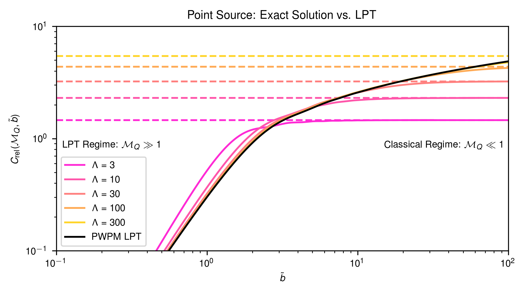
Figure 1: Dynamical friction coefficients for a point source moving in a uniform density background at fixed $\Lambda=\tilde{b}\mathcal{M}_{Q}$ as a function of the cutoff scale $\tilde{b}$. Solid colored lines plot the exact solution (Eq. 4.21), compared to the solution in LPT (plane wave, point mass, linear perturbation theory: PWPM LPT), as given in Eq. 4.26, in black. We use the plane wave, point mass linear perturbation theory curve as a reference curve in many of the other figures in the remainder of the paper. As $\tilde{b}$ becomes large at fixed $\Lambda$ ($\mathcal{M}_{Q}\ll 1$) the dynamical friction approaches the classical limit (dashed lines), which depends only on $\Lambda$ and is given above by the horizontal, dashed lines [13]. As $\tilde{b}$ becomes small for a given $\Lambda$ ($\mathcal{M}_{Q}\gg 1$) we approach the perturbation theory result (left side of the plot). This Figure is a recreation of Figure 2 from [13].

Figure 2: The density contrast, $\alpha\equiv\delta\rho/\overline{\rho}$, generated by a point-mass satellite at the origin in an asymptotically uniform FDM medium moving in the $z$-direction with relative velocity $v_{\rm rel}$, in the limit that the equations of motion can be approximated as time independent and the satellite mass is small ($\mathcal{M}_{Q}\to\infty$ or the LPT). The solution given in Eq. 4.25 is plotted here, where we set $\mathcal{M}_{Q}=1$ for simplicity; the gravitational wake behind the satellite is clearly visible.

For the special case of a point-mass satellite, the time-independent problem can actually be solved exactly, without resorting to perturbation theory. It should not be particularly surprising that this problem has been studied in some depth, as it is identical to the Coulomb scattering problem, which describes, for example, an incident beam of electrons scattered off a point-like nucleus through the Coulomb interaction [13]. In our case, the dark matter condensate plays the role of the electron beam and the satellite plays the role of the nucleus, but the mathematics (and quantum mechanics) of the attractive Coulomb potential between oppositely charged particles are identical to the universally-attractive Newtonian potential between two point masses.

The exact solution to this problem is given by the scattering states of the Coulomb potential, which can be found in a number of older quantum mechanics texts [47, 48]. The exact wave function which solves Eq. 4.1 in the time-independent regime with a gravitational potential given by Eq. 4.12, normalized so that it approaches $\sqrt{\overline{\rho}}$ at large distances, is

$$\psi(\widetilde{R},\tilde{z})=\sqrt{\overline{\rho}}\,e^{i\tilde{z}}e^{\frac{\pi}{2\mathcal{M}_{Q}}}\left|\Gamma\left(1-\frac{i}{\mathcal{M}_{Q}}\right)\right|{}_{1}F_{1}\left(\frac{i}{\mathcal{M}_{Q}},1,i\left(\sqrt{\widetilde{R}^{2}+\tilde{z}^{2}}+\tilde{z}\right)\right)\,,$$ (4.20)

where $\Gamma(x)$ is the gamma function, ${}_{1}F_{1}(a,b,c)$ is the confluent hypergeometric function [13], and the tildes represent variables in units of ${\mkern 0.75mu\mathchar 22\relax\mkern-9.75mu\lambda}$. Note that $\psi$ is a function only of $\widetilde{R}$ and $\tilde{z}$, as expected from cylindrical symmetry.

We compute the full density distribution by taking the squared norm of Eq. 4.20 and obtain the overdensity as defined in Eq. 2.1 through this density distribution. We derive the dynamical friction force experienced by the perturbing mass exactly as in Eq. 4.18. Defining $\tilde{q}\equiv\sqrt{\widetilde{R}^{2}+\tilde{z}^{2}}+\tilde{z}$, the dynamical friction coefficient is

$$C_{\rm rel}=\frac{\mathcal{M}_{Q}}{2}\,e^{\pi/\mathcal{M}_{Q}}\,\left|\Gamma\left(1-\frac{i}{\mathcal{M}_{Q}}\right)\right|^{2}\int_{0}^{2\tilde{b}}\mathrm{d}\tilde{q}\,\left|{}_{1}F_{1}\left(\frac{i}{\mathcal{M}_{Q}},1,i\tilde{q}\right)\right|^{2}\left(\frac{\tilde{q}}{\tilde{b}}-2-\log\frac{\tilde{q}}{2\tilde{b}}\right)\,.$$ (4.21)

This is the same as Equation D8 given in [13]. In Fig. 1, we compare $C_{\rm rel}$ as calculated from Eq. 4.21 with both the linear theory (equivalently derivable from Eq. 4.19 or the derivation below) and the classical limit.

As noted in Sec. 2, the LPT analysis performed in Section 4.2 applies in the regime where the quantum Mach number is much greater than 1, $\mathcal{M}_{Q}\gg 1$. In slightly more detail, we can write $\mathcal{M}_{Q}$ as

$$\mathcal{M}_{Q}\equiv\frac{v_{\rm rel}}{v_{Q}}=\frac{{\mkern 0.75mu\mathchar 22\relax\mkern-9.75mu\lambda}v_{\rm rel}^{2}}{GM}\,.$$ (4.22)

If we assume that the size of the system is some (probably large) multiple of ${\mkern 0.75mu\mathchar 22\relax\mkern-9.75mu\lambda}$ and use $v_{\rm rel}$ as a proxy for the circular velocity at some radius, then we can say $M_{\rm system}\approx A{\mkern 0.75mu\mathchar 22\relax\mkern-9.75mu\lambda}v_{\rm rel}^{2}/G$ for some dimensionless $A$. We see that $\mathcal{M}_{Q}$ is proportional to the ratio of the background system mass to the satellite mass. For a linear theory argument, we are clearly interested in the regime where this ratio is much greater than 1. One can also see from Eq. 4.22 that $\tilde{b}\mathcal{M}_{Q}=bv_{\rm rel}^{2}/GM$, where $GM/v_{\rm rel}^{2}\approx\ell_{90}$, the distance at which field particles passing by the satellite are deflected by 90^∘, as mentioned in Eq. 3.6. This is where the definition of the analogous $\Lambda$ in Fig. 1 comes from.

Expanding the hypergeometric and gamma functions in inverse powers of $\mathcal{M}_{Q}$, we have

$${}_{1}F_{1}\left(\frac{i}{\mathcal{M}_{Q}},1,iq\right) =1-\frac{{\rm Si}(q)}{\mathcal{M}_{Q}}-i\frac{{\rm Cin}(q)}{\mathcal{M}_{Q}}+\mathcal{O}\left(\mathcal{M}_{Q}^{-2}\right)$$ (4.23)

$$\Gamma\left(1-\frac{i}{\mathcal{M}_{Q}}\right) =1+\frac{i\gamma}{\mathcal{M}_{Q}}+\mathcal{O}\left(\mathcal{M}_{Q}^{-2}\right)\,,$$ (4.24)

where ${\rm Si}(q)\equiv\int_{0}^{q}\sin(t)\mathrm{d}t/t$ and ${\rm Cin}(q)\equiv\int_{0}^{q}(1-\cos(t))\mathrm{d}t/t$ are the sine and cosine integrals, respectively, and $\gamma$ is the Euler-Mascheroni constant. The corresponding density contrast is

$$\alpha(\tilde{q})=\frac{\pi-2\,{\rm Si}(\tilde{q})}{\mathcal{M}_{Q}}+\mathcal{O}\left(\mathcal{M}_{Q}^{-2}\right)\,,$$ (4.25)

which exactly matches Eq. 4.17 to machine precision to leading order in $1/\mathcal{M}_{Q}$. We plot this linear-regime overdensity in Fig. 2 in the $y-z$ plane; by cylindrical symmetry, the full three-dimensional result is obtained by rotating around the $z$-axis.

Inserting the expansion from Eqs. 4.23-4.24 into the expression for the dynamical friction in Eq. 4.21, we obtain an analytic expression for the dynamical friction coefficient in LPT:

$$C_{\rm rel}={\rm Cin}(2\tilde{b})+\frac{\sin(2\tilde{b})}{2\tilde{b}}-1+\mathcal{O}\left(\mathcal{M}_{Q}^{-1}\right)\,.$$ (4.26)

Again, this formula has been previously shown in Equation D14 of [13]. Note the dependence of the result on $\tilde{b}$, the cutoff we impose to make the integral finite. In Fig. 1, we compare this exact result with the LPT results in Sec. 4.2 and the classical limit from Sec. 3. From Fig. 1 it is clear that the exact solution approaches the perturbation theory result in the limit that $\mathcal{M}_{Q}\gg 1$, as expected.

We also refer the reader to calculations of a fixed point mass in a static FDM background with full self-gravity carried out in [49], which give rise to soliton-like solutions that resemble the ground state of the hydrogen atom in the limit that the point mass is large.

4.4 Linear Perturbation Theory: Extended Source

We would now like to generalize to the case where the satellite has an extended mass distribution, rather than simply being a point mass. We will work with the same LPT approach as in Section 4.2, starting from Eq. 4.10. We will assume a time-independent solution and take the satellite mass distribution to be a Plummer sphere [50]:

$$U_{P}=-\frac{GM}{\ell}\left(1+\left(\frac{r}{\ell}\right)^{2}\right)^{-1/2}\,.$$ (4.27)

This choice will facilitate comparison with the numerical simulations described in Sec. 5; we show in Appendix B that the qualitative features of a finite size $\ell$ do not depend sensitively on the precise mass distribution chosen. Specifically, in that Appendix, we compare the results for the Plummer sphere with that of the truncated isothermal sphere profile.

Using this potential and Fourier transforming the partial differential equation, we arrive at a slightly modified version of Eq. 4.14 for the Plummer profile,

$$\left(\frac{\hbar^{2}k^{4}}{4m^{2}}-v_{\rm rel}^{2}k_{z}^{2}\right)\tilde{\alpha}=4\pi GM\ell kK_{1}\left(\ell k\right)\,,$$ (4.28)

where $K_{1}(x)$ is the first modified Bessel function of the second kind. Changing to dimensionless variables in units of ${\mkern 0.75mu\mathchar 22\relax\mkern-9.75mu\lambda}$ gives the extended-source version of Eq. 4.15 as

$$\left(\tilde{k}^{4}-4\tilde{k}_{z}^{2}\right)\tilde{\alpha}=\frac{16\pi{\mkern 0.75mu\mathchar 22\relax\mkern-9.75mu\lambda}^{3}}{\mathcal{M}_{Q}}\tilde{\ell}\tilde{k}K_{1}(\tilde{\ell}\tilde{k})\,,$$ (4.29)

where we have also written $\ell$ relative to ${\mkern 0.75mu\mathchar 22\relax\mkern-9.75mu\lambda}$, denoted $\tilde{\ell}$ and defined in Eq. 2.9. We can then recover $\alpha$ by performing the inverse Fourier transform; our version of Eq. 4.17 is then

$$\alpha(\widetilde{\mathbf{r}})=\frac{16\pi\tilde{\ell}}{\mathcal{M}_{Q}(2\pi)^{2}}\int_{0}^{\infty}\mathrm{d}\tilde{k}_{R}\int_{-\infty}^{\infty}\mathrm{d}\tilde{k}_{z}\frac{\tilde{k}_{R}\,J_{0}(\tilde{k}_{R}\widetilde{R})\,e^{i\tilde{k}_{z}\tilde{z}}}{(\tilde{k}^{4}-4\tilde{k}_{z}^{2})}\tilde{k}K_{1}\left(\tilde{\ell}\tilde{k}\right)\,,$$ (4.30)

where $\tilde{k}=\sqrt{\tilde{k}_{R}^{2}+\tilde{k}_{z}^{2}}.$

We then carry out the $\tilde{k}_{z}$ integral in Eq. 4.30 using contour integration. The dynamical friction is given by

$$C_{\rm rel}=-2\tilde{\ell}\int\displaylimits_{0}^{\tilde{b}}\!\!\mathrm{d}\widetilde{R}\int\displaylimits^{\sqrt{\tilde{b}^{2}-\widetilde{R}^{2}}}_{0}\!\!\!\!\!\!\!\mathrm{d}\tilde{z}\int\displaylimits_{0}^{2}\!\!\mathrm{d}x\frac{\widetilde{R}\,\tilde{z}\,J_{0}\left(\sqrt{2x-x^{2}}\,\widetilde{R}\right)}{\left(\tilde{\ell}^{2}+\widetilde{R}^{2}+\tilde{z}^{2}\right)^{3/2}}\,\frac{\sin(x\tilde{z})}{\sqrt{2x}}\,K_{1}\left(\tilde{\ell}\sqrt{2x}\right)\,,$$ (4.31)

which is similar to Eq. 4.19 except for the regulation by $K_{1}(x)$. As a consistency check, we note that Eq. 4.31 becomes Eq. 4.19 in the limit where $\tilde{\ell}\to 0$.

In Fig. 3, we compare the results given by Eq. 4.31 for several values of $\tilde{\ell}$ to the LPT result given equivalently in Eqs. 4.19 and 4.26. Again, we can see graphically that the extended-source result approaches the point-source result for all values of $\tilde{b}$ as $\tilde{\ell}\to 0$. As one would expect, the extended-source result approaches the point-source result for $\tilde{b}\gg\tilde{\ell}$, where the source comes to ‘look like’ a point source. For $\tilde{b}\ll\tilde{\ell}$, we find that $C_{\rm rel}\propto\tilde{b}^{5}$, which one can verify from Eq. 4.19. One should not interpret the $\tilde{b}^{5}$ scaling as an extremely strong dynamical friction force on ‘fluffy’ objects; the dynamical friction only increases as $\tilde{b}^{5}$ for scales smaller than the size of the object. This growth is simply a cause of the response of the condensate to the presence of the satellite.

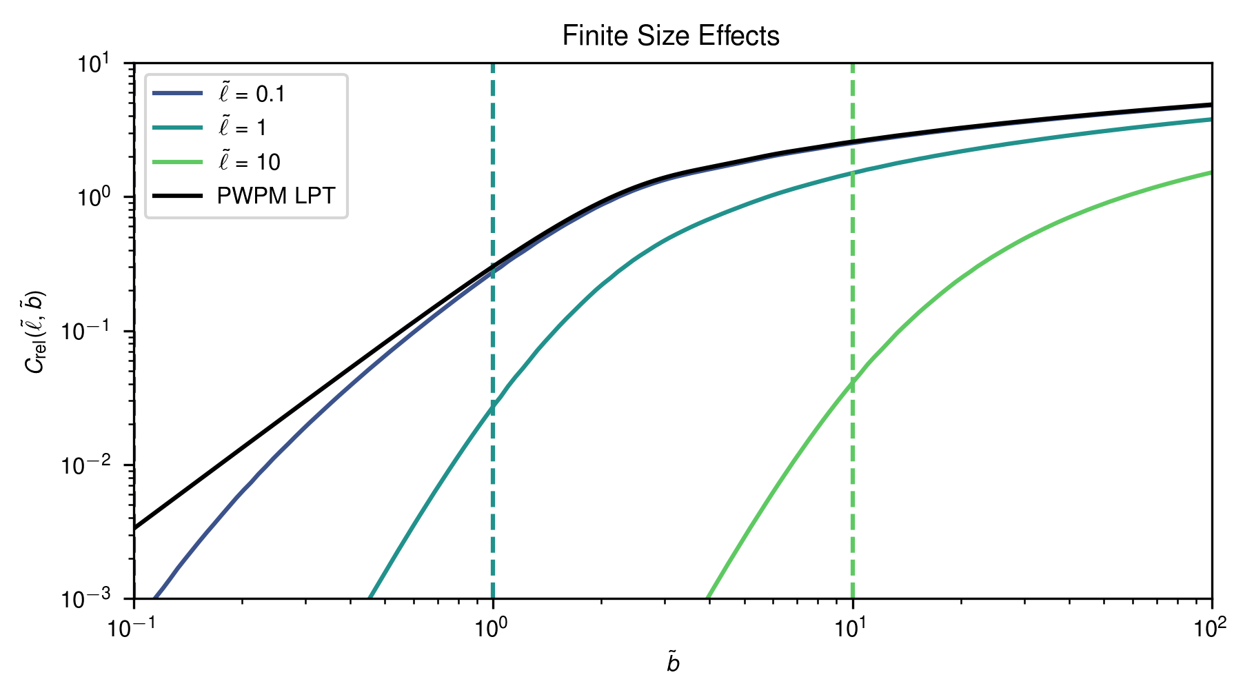
Figure 3: Effects of a finite-size satellite in the regime of linear perturbation theory, where $C_{\rm rel}$ is completely independent of the quantum mach number $\mathcal{M}_{Q}$. The perturbation theory calculation for a point mass is shown in black (PWPM LPT) along with the perturbation theory calculations for a satellite with a Plummer profile (Eq. 4.27) with varying scale length $\tilde{\ell}$ in units of the background de Broglie wavelength — these scales are also indicated by the vertical dashed lines for comparison. We can see how the finite size of the satellite suppresses dynamical friction on scales comparable to the finite size, though on scales on the order of $\sim 10^{2}$ larger, the dynamical friction only differs by a factor of order unity.

4.5 Velocity-Dispersed Condensate

In a realistic scenario, the FDM medium should have a distribution of velocities and cannot be modeled as a single plane wave, as was done above. In particular, while the core of an FDM halo may be dispersionless, the outer part of the halo is expected to have a Navarro-Frenk-White (NFW)-like profile with nonzero dispersion [13, 51]. This motivates us to investigate the behavior of the dynamical friction coefficient when the FDM medium has some velocity dispersion.

We can model this velocity dispersion by constructing the background wave function $\psi_{0}$, in analogy to Eq. 4.7, as a linear combination of plane waves [21]. In the absence of the perturbing satellite or any relative velocity, this background distribution would have a dependence on time and space given by

$$\psi_{0}(\mathbf{x},t)=\int\mathrm{d}^{3}\mathbf{k}\,\varphi(\mathbf{k})\,e^{i\mathbf{k}\cdot\mathbf{x}-i\omega(\mathbf{k})t}\,,$$ (4.32)

where the dispersion relation is given by the free Schrödinger equation:

$$\omega(\mathbf{k})=\frac{\hbar k^{2}}{2m}\,.$$ (4.33)

The function $\varphi(\mathbf{k})$ determines the distribution of velocities by weighting the individual plane waves. For an isotropic distribution, $\varphi$ is only a function of the magnitude $k$ and each plane wave is imbued with some random, uncorrelated phase shift. This behavior is expected for any realistic halo, formed through the collapse of many uncorrelated proto-halos and further randomized by violent relaxation and phase mixing [52]. This randomness would ensure that the function $\varphi(\mathbf{k})$ is a random field. We can also make the connection between $\varphi(\mathbf{k})$ and the actual velocity distribution function of the medium, $f(\mathbf{v})$, by writing

$$\left\langle\varphi(\mathbf{k})\varphi(\mathbf{k^{\prime}})\right\rangle_{\mathbf{k}}=f\left(\frac{\hbar\mathbf{k}}{m}\right)\delta(\mathbf{k}-\mathbf{k^{\prime}})\,.$$ (4.34)

For example, suppose that we would like to make our wave function mimic a classical Maxwell-Boltzmann distribution (in which case $\varphi(k)$ would be a Gaussian random field):

$$f(\mathbf{v})=\frac{\overline{\rho}}{(2\pi\sigma^{2})^{3/2}}\exp\left(\frac{-v^{2}}{2\sigma^{2}}\right)\,.$$ (4.35)

In the context of a numerical implementation where we only have a finite number of Fourier modes $\mathbf{k}_{i}$ to sum over, the coarse-grained version of Eq. 4.32 would look like

$$\psi_{0}(\mathbf{x})\propto\sum_{j}\sqrt{f(\mathbf{x},\mathbf{v}_{j})}{\rm e}^{im\mathbf{x}\cdot\mathbf{v}_{j}/\hbar+i\phi_{{\rm rand},\mathbf{v}_{j}}}\,\left(\Delta v\right)^{3/2}\,,$$ (4.36)

where the sum is over the discrete Fourier modes (which can be written equivalently in terms of $\mathbf{k}$ or the velocities $\mathbf{v}$), the phase angles $\phi_{{\rm rand},\mathbf{v}}\in[0,2\pi)$ are the manifestation of ensuring that the modes have random, uncorrelated phases, and $f(\mathbf{v})$ is the desired distribution function. The normalization is such that the average density is still $\overline{\rho}$ — see [42] for details and [53] for an example where this construction is used to model the axion dark matter field for direct-detection experiments. Eq. 4.36 shows that the classical and quantum phase space are closely related: the quantum wave function is a superposition of constant $v$ slices of the classical phase space, with amplitude $\mathbf{v}$ and random phases that give rise to interference patterns. If the initial condition had just a single velocity $\mathbf{v}_{0}$ at each location $\mathbf{x}$, then there is no interference and the classical and quantum densities agree exactly:

$$\rho(\mathbf{x})=|\psi(\mathbf{x})|^{2}=\int\left(\sqrt{f(\mathbf{x},\mathbf{v})}\right)^{2}\,\mathrm{d}^{3}\mathbf{v}\,.$$

Through the remainder of the text, when working with a medium that has a distribution of velocities, we will use an isotropic distribution of the form of Eq. 4.35, determined solely by the velocity dispersion, $\sigma$.

Such a system as described above would have a classical Mach number $\mathcal{M}_{\sigma}$ defined in Eq. 2.8. We can then describe the dynamical friction in such a velocity-dispersed medium by summing up the contributions from each plane wave, weighted by the distribution function of these plane waves [21]:

$$F_{\rm DF}=-4\pi G^{2}M^{2}\int\mathrm{d}^{3}{\mathbf{v}}\,\frac{v_{\rm rel}-\mathbf{v}\cdot\mathbf{\hat{z}}}{|\mathbf{v}_{\rm rel}-\mathbf{v}|^{3}}\,f(\mathbf{v})\,C_{\rm rel,pw}\left(\mathcal{M}_{Q},\tilde{b}\right)\,,$$ (4.37)

where the $C_{\rm rel,pw}(\mathcal{M}_{Q},\tilde{b})$ is the dimensionless dynamical friction coefficient for a plane wave, which in general depends on both the quantum Mach number and the cutoff scale of interactions. In practice, one can plug in either a fully non-linear function for $C_{\rm rel,pw}(\mathcal{M}_{Q},\tilde{b})$ such as Eq. 4.21, or the LPT theory Eq. 4.26, or even include finite-size effects by using Eq. 4.31, we leave this treatment to future work. Taking the distribution function to be Maxwellian, and changing variables to the dimensionless velocity $\tilde{\mathbf{v}}=\mathbf{v}/v_{\rm rel}$, we may state the above in terms of the dynamical friction coefficient as

$$C_{\rm rel}=-\frac{\mathcal{M}_{\sigma}^{3}}{(2\pi)^{3/2}}\int\mathrm{d}^{3}\tilde{\mathbf{v}}\,\frac{1-\tilde{\mathbf{v}}\cdot\mathbf{\hat{z}}}{|\mathbf{\hat{z}}-\tilde{\mathbf{v}}|^{3}}\,\exp\left(-\frac{u^{2}}{2}\mathcal{M}_{\sigma}^{2}\right)C_{\rm rel,pw}\left(\mathcal{M}_{Q},b\right)\,,$$ (4.38)

where, again, $C_{\rm rel,pw}\left(\mathcal{M}_{Q},b\right)$ is the dynamical friction coefficient in the case of a plane wave, and $C_{\rm rel}$ is the overall dynamical friction coefficient in the velocity-dispersed case.

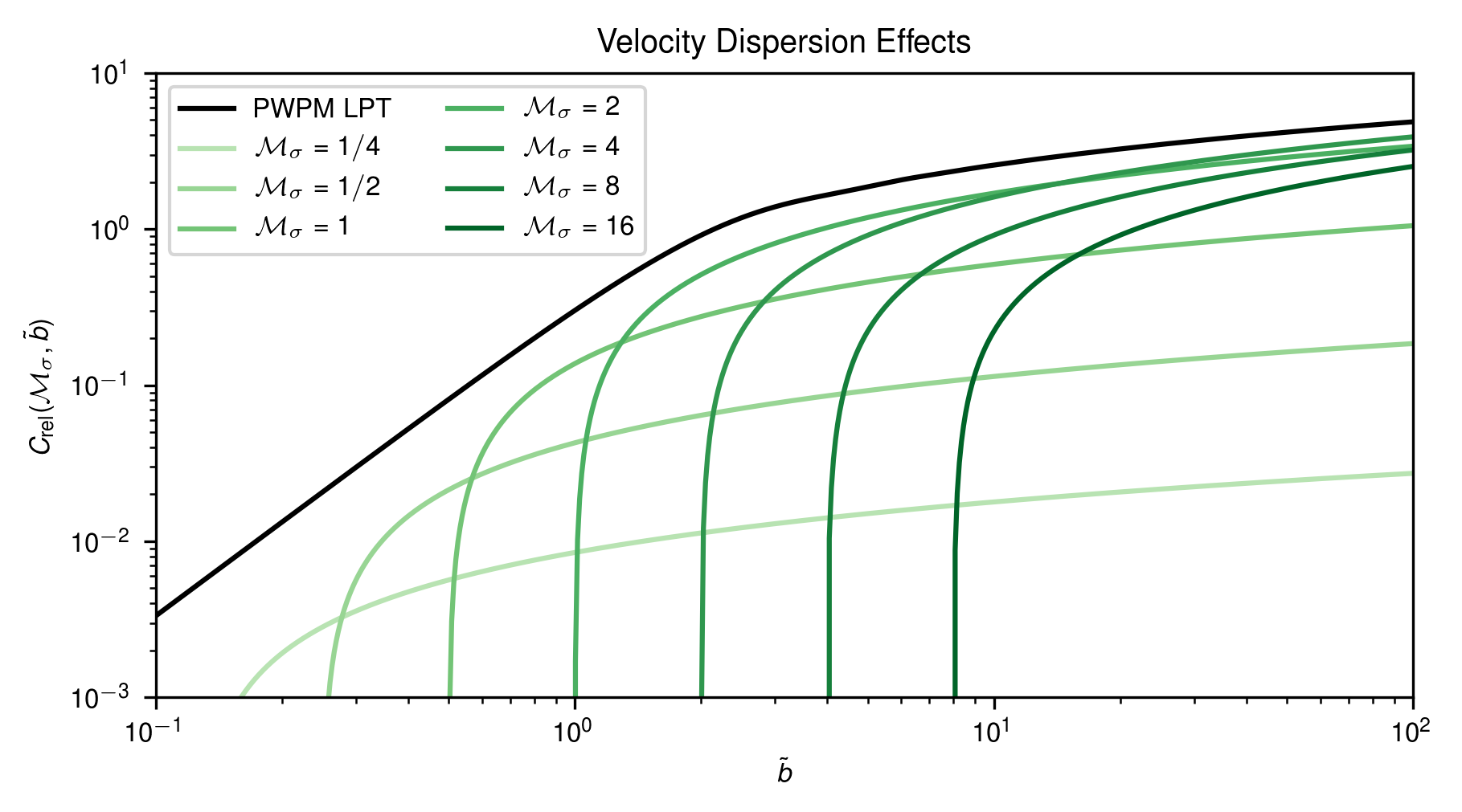
Figure 4: The dynamical friction coefficient $C_{\rm rel}$ for a point source, as derived using linear perturbation theory (LPT) and defined in Eq. 4.26, is shown in black. The green curves represent the coefficient as calculated by Eq. 4.39 for several different values of the classical Mach number $\mathcal{M}_{\sigma}$. See text for a detailed discussion of the effects shown here.

As we touched on in Sections 4.2 and 4.3, when $\mathcal{M}_{Q}\ll 1$ the time-independent dynamical friction calculation for a point source approaches the classical answer. However, in the limit of LPT, when $\mathcal{M}_{Q}\gg 1$, we can apply our perturbation theory argument to replace $C_{\rm rel,pw}$ above. Using these assumptions, along with the assumption that the cutoff scale $\tilde{b}$ is much larger than the dispersion de Broglie wavelength ${\mkern 0.75mu\mathchar 22\relax\mkern-9.75mu\lambda}_{\sigma}$, one can show [21] that the dynamical friction is given by

$$C_{\rm rel}=\mathcal{M}_{\sigma}^{2}\log\left(\frac{2\tilde{b}}{\mathcal{M}_{\sigma}}\right)\mathbb{G}\left(\frac{\mathcal{M}_{\sigma}}{\sqrt{2}}\right)\,,$$ (4.39)

where $\mathbb{G}(X)$ is defined in Eq. 3.8. Indeed, this result is the same as the classical Chandrasekhar result [33, 37] except with the Coulomb logarithm defined in terms of $\mathcal{M}_{\sigma}$. In Fig. 4, we compare the dynamical friction found in this case to that found in the case of a point mass in a uniform medium as given in Eq. 4.26. We can see that the formula given here breaks down when $b<{\mkern 0.75mu\mathchar 22\relax\mkern-9.75mu\lambda}_{\sigma}$, or, when $b$ is expressed in units of ${\mkern 0.75mu\mathchar 22\relax\mkern-9.75mu\lambda}$, $\tilde{b}<\mathcal{M}_{\sigma}$. We expect the velocity-dispersed solution to approach the point-source LPT solution in the limit that $\sigma\to 0$, or equivalently $\mathcal{M}_{\sigma}\to\infty$. However, this also implies that the de Broglie wavelength corresponding to the velocity dispersion ${\mkern 0.75mu\mathchar 22\relax\mkern-9.75mu\lambda}_{\sigma}=\hbar/m\sigma$ becomes very large, and the assumption that $b\gg{\mkern 0.75mu\mathchar 22\relax\mkern-9.75mu\lambda}_{\sigma}$ is no longer valid. In this regime, we can assume that ${\mkern 0.75mu\mathchar 22\relax\mkern-9.75mu\lambda}_{\sigma}$ is so large that we essentially have a uniform density background.

In practice, then, care must be taken to consider the comparative size of ${\mkern 0.75mu\mathchar 22\relax\mkern-9.75mu\lambda}_{\sigma}$ and the size of the system $b$. The results derived in this section only apply in the case that $b\gg{\mkern 0.75mu\mathchar 22\relax\mkern-9.75mu\lambda}_{\sigma}$. On the other hand, when $b\ll{\mkern 0.75mu\mathchar 22\relax\mkern-9.75mu\lambda}_{\sigma}$, we may apply the uniform density results. In the intermediate regime of $b\approx{\mkern 0.75mu\mathchar 22\relax\mkern-9.75mu\lambda}_{\sigma}$, individual over-densities and under-densities can strongly influence the satellite’s motion, and the true dynamical friction force becomes uncertain. The calculation behind Eq. 4.39 assumes that these over-/under-densities can be treated in a statistically averaged way, so it does not take this effect in to account. This is why we do not see any strange behavior at $\tilde{b}\approx\mathcal{M}_{\sigma}$ in Fig. 4.

5 Numerical Simulations

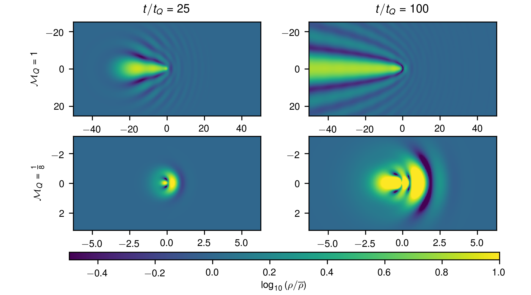
Figure 5: Density contrast in the $x=0$ plane at various time steps of our simulations, for a satellite moving in the $\mathbf{\hat{z}}$ direction, which points towards the right. The density scale is logarithmic and all plots are on the same scale. The simulations shown here have zero background velocity dispersion and a satellite with size $\ell/L_{Q}=0.5$, the smallest size we explore numerically and thus the closest to a point mass. The panels on the left show a snapshot of the simulations at earlier times, with later times in the right panel. The top panels show a simulation at a quantum Mach number of $\mathcal{M}_{Q}=1$ while the bottom panels show $\mathcal{M}_{Q}=0.125$. We see that at higher Mach number, the resulting wake is much less dense, indicative of the decrease in the dynamical friction. Spatial scales are indicated in units of ${\mkern 0.75mu\mathchar 22\relax\mkern-9.75mu\lambda}$, where the horizontal axis is the $z$-axis and the vertical axis is the $y$ axis.

Figure 6: Density contrast as in Fig. 5, but for the case of a background medium with some finite velocity dispersion. $\mathcal{M}_{\sigma}=4$ for all four panels and all other parameters are the same as Fig. 5. Spatial scales are in units of ${\mkern 0.75mu\mathchar 22\relax\mkern-9.75mu\lambda}$. Note that the logarithmic density scale for these plots is different than Fig. 5.

Now that we have explored the analytic results in different regimes, we move on to numerically calculate the time-dependent solutions in each of these regimes and compare them to the analytic results. We carry out time-dependent numerical simulations of the response of the wave function to a massive satellite with a Plummer mass density profile in order to measure the dynamical friction coefficient as a function of dimensionless parameters $\mathcal{M}_{\rm Q}$, $\tilde{\ell}$, and $\mathcal{M}_{\sigma}$ using the unitary spectral method of [20]. See Appendix C for details of the numerical implementation, which solves Eq. 4.1.

The perturbing satellite moves through half the distance of a periodic box of size $L_{\rm box}=64\pi L_{\rm Q}$. In this amount of time, the simulation is unaffected by the boundary conditions. Our numerical resolution is $512^{3}$ grid points. We simulate $65$ different relative velocities, corresponding to choices of $\mathcal{M}_{\rm Q}$ in $[0,2]$. We also simulate four different satellite sizes given by the Plummer profile, defined with respect to the quantum length scale as $\ell/L_{Q}=\frac{1}{2},1,2,4$. Finally, we simulate three different cases of background velocity dispersion, again defined with respect to the quantum length scale as ${\mkern 0.75mu\mathchar 22\relax\mkern-9.75mu\lambda}_{\sigma}/L_{Q}=\infty,8,4$, where $\infty$ corresponds to no velocity dispersion. This results in running a total of $780$ simulations. We verified that our solutions are numerically converged by comparing with simulations at $256^{3}$ resolution. For the velocity-dispersed simulations, we run ten additional simulations for each Mach number and satellite size, with different initial random phases, in order to obtain an ensemble average for the calculation of the dynamical friction.

In Fig. 5, we show representative slices through the plane $x=0$ for a few of our simulations that do not contain any velocity dispersion. The morphological similarities between these slices and the solution for the time-independent LPT result in Fig. 2 further increases our confidence in both results. We can also see from the $\mathcal{M}_{Q}=1/8$ simulations that the deviation from the LPT solution is significant at small $\mathcal{M}_{Q}$, as we expect.

In Fig. 6, we show a version of Fig. 5 except now with some finite velocity dispersion, specifically $\mathcal{M}_{\sigma}=4$. Here, we can see how the overdensities induced in the fluid from the finite velocity dispersion act to disrupt the gravitational wake and therefore decrease the effect of dynamical friction.

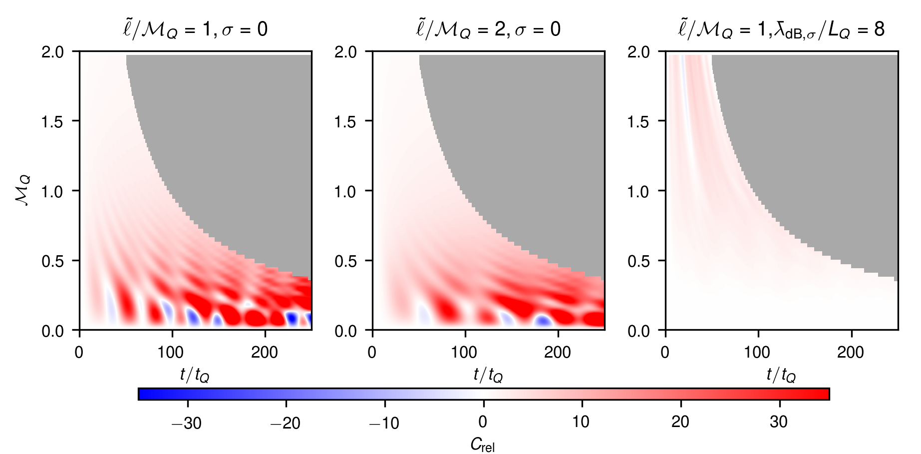
Figure 7: The instantaneous dynamical friction $C_{\rm rel}$ (defined in Eq. 2.11) as both a function of time and Mach number $\mathcal{M}_{Q}$ from our simulations. Across the three panels, we vary the size of the satellite relative to $L_{Q}$ and the presence of velocity dispersion in the background medium. The gray areas at the top right of each panel indicate where the satellites have traveled half the length of the simulation domain, and we therefore stop tracking the evolution. Left Panel: Fiducial case of no background velocity dispersion and a satellite size $\ell/L_{Q}=1$. Middle Panel: Same as the left panel, but with a satellite of twice the size. Right Panel: Same as the left panel, but with a velocity dispersion ${\mkern 0.75mu\mathchar 22\relax\mkern-9.75mu\lambda}_{{\rm dB},\sigma}/L_{Q}=8$ (see Sec. 2 for definitions).

6 Interpretation of Numerical Simulations

We extract dynamical friction coefficients as a function of time in our simulations of a finite-size satellite traveling with Mach number $\mathcal{M}_{Q}$ in constant and velocity-dispersed backgrounds. These were obtained by integrating the gravitational force of the perturbed dark matter density field acting on the satellite, taking into account the satellite’s extended mass distribution as well; implementation details are found in Appendix C. Fig. 7 shows the instantaneous dynamical friction coefficients for three different setups and Mach numbers $0\leq\mathcal{M}_{Q}\leq 2$. The three setups compare a fiducial case of an object of size $\ell/L_{Q}=1$ and no velocity dispersion $\sigma=0$ against a larger extended object of size $\ell/L_{Q}=2$ as well as with a velocity-dispersed background with dispersion ${\mkern 0.75mu\mathchar 22\relax\mkern-9.75mu\lambda}_{\sigma}/L_{Q}=8$.

The overall growth of the drag force is logarithmic in time, as expected from time-independent analytic theory. But a key feature of the time-dependent dynamical friction coefficients are oscillations. The duration of these oscillations occurs on the scale of the satellite size: it is seen in Fig. 7 that the period of oscillations approximately doubles in time when the satellite size is doubled. The size of the oscillations are strongest at low quantum Mach numbers $2\pi\mathcal{M}_{Q}\sim 1$. The overall dynamical friction force is also strongest at $2\pi\mathcal{M}_{Q}\sim 1$, and sharply drops to $0$ at $\mathcal{M}_{Q}=0$ which is when the object is at rest with respect to the medium. We note that the oscillations may be large enough at low quantum Mach numbers that the dynamical friction drag force can instantaneously be negative at times, e.g., when an interference crest ahead of the satellite pulls the satellite forward. However, on average, the addition of velocity dispersion in the background reduces the drag force, as the background interferes with the wake.

Below, we will compare a number of time-independent expressions for the dynamical friction in a given situation to the time-dependent simulations that we have run. This comparison, a priori, does not seem physical. However, we know that the time-independent calculations depend upon the dynamical friction cutoff scale $\tilde{b}$. We also know that, absent the quadratic dispersion relation given in Eq. 4.33, we can think of the wake forming outwardly from the satellite propagating roughly at a speed $v_{\rm rel}$. Thus we can treat the scale $v_{\rm rel}t$ as a stand-in for the cutoff scale $b$ that we use in our time-independent calculations, similar to the formalism of [36].

With this in mind, all of the comparisons discussed below will give the total dynamical friction in the simulation at time $t$ and relate it to the time-independent calculation integrated out to the cutoff scale $v_{\rm rel}t$. This scale will simply be referred to by the variable $b$ for the cutoff scale (typically in units of ${\mkern 0.75mu\mathchar 22\relax\mkern-9.75mu\lambda}$, indicated by $\tilde{b}$).

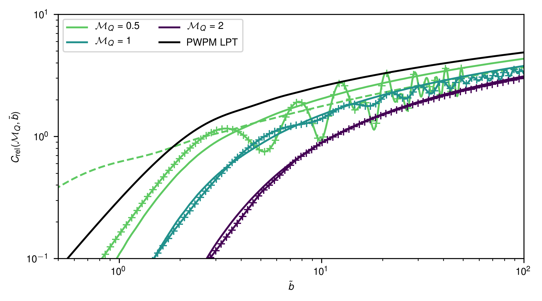
Figure 8: Dynamical friction coefficient $C_{\rm rel}$ as computed from LPT in Eq. 4.31 (solid lines), along with the values calculated in our simulations (‘+’ marks), for several different values of the quantum Mach number $\mathcal{M}_{Q}$. For the most strongly non-linear case ($\mathcal{M}_{Q}=0.5$) we also include the $C_{\rm rel}$ calculated from the exact solution for a point source (Eq. 4.21) with $\mathcal{M}_{Q}=0.5$ (dashed line). In our simulations, $\tilde{b}$ is associated with $v_{\rm rel}t$, as described in the text. All of the above pertain to a finite-size satellite with $\ell/L_{Q}=1$. We also show the LPT result for a point source as computed from Eq. 4.26 (black solid line). The LPT result for extended sources matches the $\mathcal{M}_{Q}=2$ simulation to better than 3% for $\tilde{b}\gtrsim 7$. For the non-linear case of $\mathcal{M}_{Q}=0.5$, it is clear that the exact point mass formula (Eq. 4.21) better matches the mean behaviour of the simulations. However, it clearly does not capture the significant oscillations away from this mean behavior, which are most likely due to the simulations taking place over a finite time, whereas Eq. 4.21 is computed in an infinite-time limit.

6.1 Comparison of Finite-Size Calculations to Simulations

Beginning first with the case of zero velocity dispersion, we investigate the accuracy of the LPT for finite-size satellites as discussed in Section 4.4. We expect our results to be most accurate in the LPT regime where $\mathcal{M}_{Q}\gg 1$, which is probed only to a limited extent by the simulations that we have run in this work, due to numerical resolution limitations. The results of this comparison can be seen in Fig. 8.

As expected, the LPT predictions perform exceedingly well against the simulations at higher Mach number. In particular, the $\mathcal{M}_{Q}=2$ case agrees to better than 3% for $\tilde{b}\gtrsim 7$. This case corresponds to $\tilde{\ell}=2$, since the simulations in Fig. 8 all have a satellite size of $\ell=L_{Q}$. On the other hand, in the non-linear regime of $\mathcal{M}_{Q}=0.5$, we see that while the LPT predicts the general trend of the dynamical friction force quite well, the true dynamical friction fluctuates much more strongly than the LPT case. The LPT result also tends to systematically overestimate the dynamical friction force in this non-linear regime, by a factor that becomes larger as one moves deeper into the non-linear regime. In the weakly non-linear regime of $\mathcal{M}_{Q}=0.5$ that is shown in Fig. 8, the over-estimate of $C_{\rm rel}$ is only of order unity.

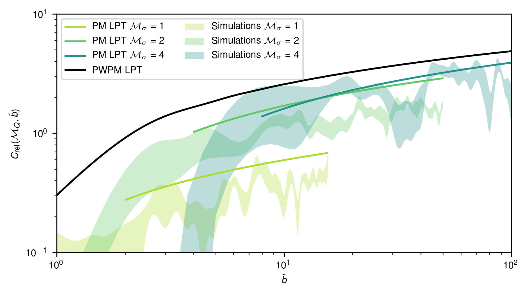
Figure 9: Dynamical friction coefficient $C_{\rm rel}$ as computed from Eq. 4.39 using LPT for a velocity-dispersed medium (solid lines), along with the values calculated in our simulations (shaded regions), for several different values of the quantum Mach number $\mathcal{M}_{Q}$. The shaded regions indicate the one-standard-deviation range of dynamical friction forces over the ensemble of simulations for a given $\mathcal{M}_{Q}$, with the other parameters set to $\ell/L_{Q}=1$ and $v_{Q}/\sigma=4$. Note that while the simulations are fully non-linear and use finite-size satellites, we are comparing to the theory for a point mass in the linear regime, and only show these analytic results in the regime $\tilde{b}>2\mathcal{M}_{\sigma}$ where they are applicable.

6.2 Comparison of Velocity-Dispersed Calculations to Simulations

We can also compare our simulations of dynamical friction in a velocity-dispersed FDM medium to the theory that we have developed for that scenario in Section 4.5. When making this comparison, we must keep in mind that any individual realization of a velocity-dispersed FDM medium will have a particular set of over- and under-densities (see Fig. 6) that will affect the temporal evolution of the dynamical friction. As mentioned in Section 5, we mitigate these effects by running an ensemble of simulations for a given set of parameters ($\mathcal{M}_{Q}$, $\mathcal{M}_{\sigma}$, $\mathcal{\ell}$) and then comparing our analytic theory with the range of values within one standard deviation over the ensemble of simulations. This comparison is shown in Fig. 9 for $\ell/L_{Q}=1$, $v_{Q}/\sigma=4$, and $\mathcal{M}_{Q}=0.25,0.5,1$.

While the simulations are of course fully non-linear in their treatment of the dynamical friction force and use finite-size satellites, we compare these simulations to the theory developed for point masses in a linear regime as given in Eq. 4.39. Nonetheless, the analytic results give decent agreement with the simulations. In particular, for $\mathcal{M}_{Q}=1$ which is the closest to the linear regime for the simulations shown, Eq. 4.39 does quite well at capturing the trends in the simulations. However, as with the results of Section 6.1, we see that the LPT results overestimate the dynamical friction force in the non-linear regime ($\mathcal{M}_{Q}=0.5$ here). Some of this difference could also be due to finite-size effects. These simulations have $\tilde{\ell}=0.5$, respectively, which corresponds to the $\mathcal{M}_{Q}=0.5$ cases shown in Fig. 8, from which we can see that the inclusion of finite size only changes the resulting dynamical friction force by a factor of order unity for $\tilde{b}\gtrsim 10$.

7 Applications to Astrophysical Systems

Now that we have thoroughly investigated the theory of dynamical friction in a universe composed of FDM, we would like to apply the theory to a few systems of interest. To do this, we must first identify the systems we are interested in and determine in what regime of dynamical friction they reside. Towards that end, we may refer to the formulae for inferring the scale of the dimensionless parameters of interest, namely $\mathcal{M}_{Q}$, $\mathcal{M}_{\sigma}$, and $\tilde{\ell}$, given in Section 2. It is important to note here that the regime that especially lies outside the validated regime of any analytic theory we have developed here is $\mathcal{M}_{Q}\approx\mathcal{O}(1/2\pi)$, based on our simulations. This restriction is equivalent to:

$$\left(\frac{M}{10^{9}\,M_{\odot}}\right)\left(\frac{m}{10^{-22}\,{\rm eV}}\right)\left(\frac{100\,{\rm km}\,{\rm s}^{-1}}{v_{\rm rel}}\right)\sim 1$$ (7.1)

Below we will treat the cases of the globular clusters around Fornax in depth, and illustrate why many massive satellites such as the Sagittarius dwarf and the Magellanic Clouds are likely well-described by the classical Chandrasekhar formula. The infall of supermassive black holes (SMBH) in an FDM halo has already been thoroughly discussed in [13] and [21], though our estimate above of the regime in which detailed simulations may be warranted suggests that it may be worth revisiting this case as well.

7.1 Fornax Globular Clusters

The Fornax dwarf spheroidal (dSph) galaxy is the most massive galaxy of its type orbiting the Milky Way (that shows no strong signs of tidal disruption) and has thus been extensively studied in the literature [54, 55, 56, 57, 58, 59, 60, 61, 62, 63]. The tendency for dSph galaxies to be heavily dynamically dominated by dark matter [64, 65, 66] has made them ideal test beds for the nature of dark matter on cosmologically small scales [67, 6].

One of Fornax’s unique features is the set of six globular clusters associated with it [57, 68]. These globular clusters have long puzzled astronomers as they all appear to be old ($\sim$10 Gyr), yet dynamical friction calculations show that globular clusters with similar orbits should have long ago sunk to the center of the Fornax dSph, assuming that they had been in these orbits for a significant fraction of their lifetimes [26, 69, 70, 71, 57]. Specifically, the classical treatment of the problem as first raised in [26] and subsequently discussed in [69, 70] indicated that the timescale for the infall of the globular clusters around Fornax to the center of the dSph due to dynamical friction should be on the order of $\tau_{\rm DF}\sim 1\,$Gyr [70], which is much shorter than the proposed age of the dSph of $\sim 10\,$Gyr [72, 73]. If the clusters are in fact still infalling, it seems extremely unlikely that we would happen to observe them all just before they fall into the center of Fornax. This issue has come to be known as the timing problem [26, 25].

There have been multiple proposed solutions to this problem, such as tidal effects of the Milky Way, a population of massive black holes which act to dynamically heat the clusters [70], non-standard dark matter models (such as we investigate here) [62], alterations to the dark matter distribution in the Fornax dSph [57], and more complicated treatments of the dynamical friction problem beyond a Chandrasekhar-type formula [33, 71, 62, 74]. We mention these arguments for the interested reader, but will not reiterate them here. Instead, we will focus on the extent to which FDM may be able to independently solve this problem.

Following the approach of [13], we will estimate the infall time of each globular cluster due to dynamical friction, $\tau_{\rm DF}$, as the angular momentum of the globular cluster’s orbit divided by the torque due to dynamical friction. Assuming that each globular cluster is on a circular orbit, this time is given by

$$\tau_{\rm DF}=\frac{L}{r|F_{\rm DF}|}=\frac{v_{\rm rel}^{3}}{4\pi\overline{\rho}G^{2}MC_{\rm rel}}\,,$$ (7.2)

where $v_{\rm rel}$ is the circular orbit velocity, $\overline{\rho}$ is the local density of dark matter at the position of the given globular cluster, $M$ is the mass of the globular cluster, $G$ is Newton’s constant, and $C_{\rm rel}$ is as defined in Eq. 2.12.

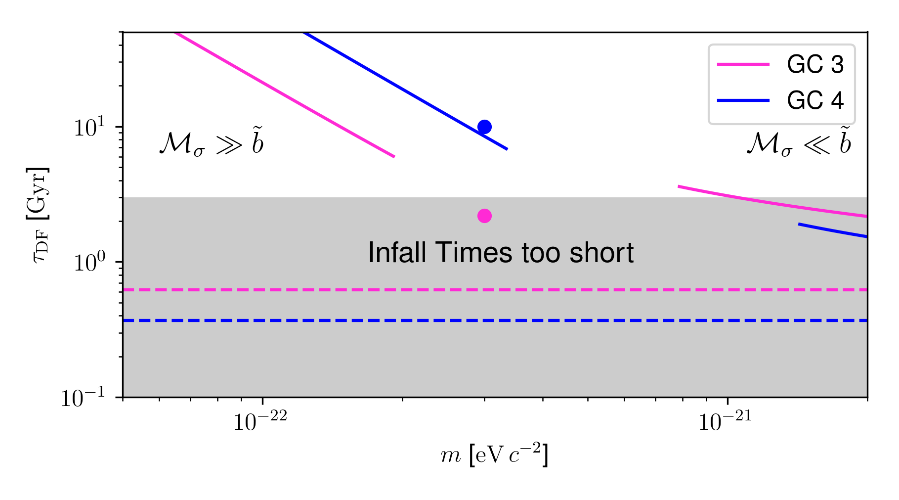
Figure 10: Infall times as a function of FDM particle mass for the two Fornax globular clusters with the shortest infall times, GC 3 and GC 4. The grey shaded region indicates $\tau_{\rm DF}<3\,$Gyr, roughly the region in which a timing problem exists. The horizontal dashed lines indicate the infall times in a $\Lambda$CDM universe as calculated in [13], which we can see clearly lies well within the timing-problem domain. The points indicate the infall times in an FDM scenario calculated by [13] for $m=3\times 10^{-22}\,{\rm eV}$ using Eq. 4.26. The solid lines indicate our estimates for the infall times in the FDM scenario where Eq. 4.26 is applied at the left-hand side of the plot and Eq. 4.39 is applied at the right-hand side of the plot. The break between the solid lines indicates the region where the velocity dispersion de Broglie wavelength is on the order of the size of the system and individual over- and under-densities make $\tau_{\rm DF}$ quite uncertain/stochastic. Our estimates differ from those of [13] (points) in that we use updated constraints on the dynamic properties of the Fornax dSph. Additionally, the [13] estimates are simply extrapolations of the point-mass LPT curves (curves shown on the left hand side of the plot) whereas we make sure to apply this theory only in the appropriate regime.

To estimate the infall time, we must determine the correct formula to use to calculate $C_{\rm rel}$. The typical size of the globular clusters in the Fornax dSph system is about $\ell\sim 2\,{\rm pc}$, they have a typical mass of about $M\sim 2\times 10^{5}\,M_{\odot}$, and a typical orbital velocity of $\sim 10\,{\rm km}\,{\rm s}^{-1}$ (assuming an isotropic velocity distribution) [57, 75, 76]. Though the distances from the center of the Fornax dSph vary over the collection of globular clusters, we will take the typical globular cluster to be located at the core radius of the King profile fit to the Fornax dSph, which is $r\approx 668\,{\rm pc}$ [77]. The density of dark matter at this radius has been estimated to be $\overline{\rho}\approx 2\times 10^{7}\,M_{\odot}\,{\rm kpc}^{-3}$ [78] and the velocity dispersion of the dark matter at this radius (estimated from the velocity dispersion of the stars) is $\sigma\approx 10\,{\rm km}\,{\rm s}^{-1}$ [77].

With these numbers in mind, we can calculate the dimensionless parameters of interest:

$$\tilde{\ell}\approx 1.04\times 10^{-3}\left(\frac{m}{10^{-22}\,{\rm eV}}\right)\ \ ,\ \ \tilde{b}\approx 3.47\times 10^{-1}\left(\frac{m}{10^{-22}\,{\rm eV}}\right)\ \$$ (7.3)

$$\mathcal{M}_{Q}\approx 90\left(\frac{m}{10^{-22}\,{\rm eV}}\right)^{-1}\ \ ,\ \ \mathcal{M}_{\sigma}\approx 1\,.$$ (7.4)

We can immediately see that we are almost always in the LPT regime ($\mathcal{M}_{Q}\gg 1$) and that the globular clusters can be accurately treated as point masses ($\tilde{b}\gg\tilde{\ell}$). At low FDM mass, the de Broglie wavelength of the velocity dispersion is much greater than the size of the system ${\mkern 0.75mu\mathchar 22\relax\mkern-9.75mu\lambda}_{\sigma}\gg b$ (or equivalently, $\mathcal{M}_{\sigma}\gg\tilde{b}$) and we may treat the background as constant density, applying Eq. 4.26 for $C_{\rm rel}$ in Eq. 7.2. At high FDM mass, we are in the opposite regime, $\mathcal{M}_{\sigma}\ll\tilde{b}$, and the inhomogeneities caused by the velocity dispersion are very small compared to the size of the system, so we may accurately apply Eq. 4.39. However, between these two regimes, the precise dynamical friction force will be strongly affected by the presence or absence of single over-densities/under-densities in the FDM caused by the velocity dispersion. In this regime, the infall time is uncertain.

We estimate the infall times for the two Fornax globular clusters with the shortest infall times (for which the timing problem is most severe). We use information on the mass $M$, projected radial distance from the center of the Fornax dSph $r_{\perp}$, and core sizes $\ell$ taken from [57, 75, 77]. These are the same parameters as used in [13]. Following the procedure of [13] further, we take the true radial distance of the globular clusters from the center of the Fornax dSph to be $r=2r_{\perp}/\sqrt{3}$ and then take the velocity dispersion curve to be roughly flat at $\sigma\approx 10\,{\rm km}\,{\rm s}^{-1}$ [57, 78]. We also take the globular clusters to be on circular orbits, with velocities determined as $v_{\rm rel}=\sqrt{GM_{\rm encl}(r)/r}$, where $M_{\rm encl}(r)$ is the mass of the Fornax dSph contained within the radius $r$. However, unlike [13], we use updated fits to the mass and density profiles of the Fornax dSph taken from [78] and we only apply Eq. 4.26 when $\mathcal{M}_{\sigma}>2\tilde{b}$, using Eq. 4.39 when $\mathcal{M}_{\sigma}<\tilde{b}/2$. As argued above, in the regime $\tilde{b}/2<\mathcal{M}_{\sigma}<2\tilde{b}$, the dynamical friction force is made uncertain by the presence of individual over-densities in the FDM, so we do not make a prediction for the infall time.

We show the results of this calculation in Fig. 10. It is clear that for FDM masses $m\gtrsim 10^{-21}\,{\rm eV}$, FDM no longer resolves the timing problem. It should also be noted that as $m$ becomes larger we will move first into the non-linear regime ($\mathcal{M}_{Q}\sim 1$) where our LPT calculations do not apply and one must be careful applying analytic arguments. As $m$ grows larger, we will move in to the classical regime ($m\to\infty$ or $\mathcal{M}_{Q}\ll 1$) where we may apply the classical Chandrasekhar formula. One must be aware of these different regimes when evaluating whether dynamical friction changes significantly in the FDM picture.

7.2 The Sagittarius Stream

The Sagittarius (Sgr) stream is a massive stellar stream that consists of the tidal debris of one of the Milky Way’s most massive recent accretion events  [79, 80, 81, 82, 83, 84, 85, 86, 87, 88, 89, 90]. A recent review of the literature is given in [87] with important, more recent, contributions in [88, 89, 90]. Dynamical modeling of the Sgr orbit can constrain the shape of the Galactic potential, and therefore the structure, of our Galaxy [80, 84, 85, 88, 90].

It has long been known that Sgr’s orbit depends sensitively on the effects of dynamical friction [91], making various families of orbital parameters viable for different ranges of initial masses for Sgr. Here, we simply make an estimate of the dimensionless parameters which determine the applicable theory for $C_{\rm rel}$, as a guide for future work investigating the infall of Sgr in an FDM universe.

To do this, we follow the orbital model of [88], taking the initial scale-size of Sgr (upon first infall) as $\ell=25\,{\rm kpc}$, the initial mass as $M_{\rm Sgr}=1.3\times 10^{10}\,M_{\odot}$, the initial distance from the center of the Milky Way as $d_{\rm init}=125\,{\rm kpc}$, and the initial velocity relative to the center of the Milky Way as $v_{\rm init}=72.6\,{\rm km}\,{\rm s}^{-1}$. Using these parameters, we infer

$$\mathcal{M}_{Q}=2.49\times 10^{-2}\left(\frac{m}{10^{-22}\,{\rm eV}}\right)^{-1}\ \ ,\ \ \tilde{\ell}=94.7\left(\frac{m}{10^{-22}\,{\rm eV}}\right)\ \ ,\ \ \tilde{b}=473\left(\frac{m}{10^{-22}\,{\rm eV}}\right)\,.$$ (7.5)

We can see that the large mass of the Sgr dwarf puts this problem strongly outside the regime of LPT, but most likely into the regime where classical arguments should still be viable ($\mathcal{M}_{Q}\ll 1$). Additionally, the size of the Sgr dwarf is large enough to play an important role in reducing the dynamical friction significantly.

Recent studies enabled by the data provided by the Gaia satellite [92, 93] have allowed authors to look at the shape of the velocity ellipsoid of the Milky Way’s stellar halo out to large Galactocentric radii [94, 95]. This allows us to estimate the final dimensionless parameter of interest, the classical Mach number $\mathcal{M}_{\sigma}$. Taking the one-dimensional velocity dispersion at Galactocentric radii of $r=125\,{\rm kpc}$ to be $\sigma\approx 80\,{\rm km}\,{\rm s}^{-1}$ [94], we see that $\mathcal{M}_{\sigma}\approx 1$, meaning that the finite velocity dispersion should be important, especially as the system is large. The parameter estimates above indicate that for most values of $m$ that are of interest, classical dynamical friction arguments should still accurately describe the orbit of Sagittarius.

7.3 The Magellanic Clouds

The Magellanic Clouds, consisting of the Large Magellanic Cloud (LMC) and the Small Magellanic Cloud (SMC), are some of the most massive satellites of the Milky Way and have been studied in depth in the literature [96, 97, 98, 99, 100, 101]. Dynamical friction has a very important role to play in the orbit of the Magellanic Clouds around the Milky Way, as was recently shown in [99] using high-resolution $N$-body simulations in a universe with ‘traditional’ CDM. In these simulations, the authors of [99] were able to show that the dark matter wake created by the infall of the LMC should have observable effects on the outer parts of the stellar halo.

Since the form of the DM wake formed in the FDM paradigm is so drastically different, we would of course expect the observable effects to change in the FDM scenario. Similarly as for Sgr, we aim here to estimate the values of the dimensionless parameters of interest to determine in what regime it lies. To this end, we take parameters for the LMC from [99], using a scale size of $\ell\approx 20\,{\rm kpc}$, a total mass of $M_{\rm LMC}\approx 2\times 10^{11}\,M_{\odot}$, and a total orbital velocity of $v_{\rm rel}\approx 325\,{\rm km}\,{\rm s}^{-1}$ gives us the dimensionless parameters of interest:

$$\mathcal{M}_{Q}=7.24\times 10^{-3}\left(\frac{m}{10^{-22}\,{\rm eV}}\right)^{-1}\ \ ,\ \ \tilde{\ell}=340\left(\frac{m}{10^{-22}\,{\rm eV}}\right)\ \ ,\ \ \tilde{b}=848\left(\frac{m}{10^{-22}\,{\rm eV}}\right)\,.$$ (7.6)

As we can see, this system, like Sgr, lies deeply in the non-linear regime, and the finite size of the system is large enough to play a significant role in altering the dynamical friction. The LMC system is in a regime where the classical Chandrasekhar formula will well-approximate the net dynamical friction on the object. However, the de Broglie wavelength of the relative motion of the system is not negligible: ${\mkern 0.75mu\mathchar 22\relax\mkern-9.75mu\lambda}\sim 60\,{\rm pc}$, and the gravitational wake will have transient structures on this length scale, which may have observable effects.

Physical Setup	Exact PM	LPT PM	LPT EM	LPT VD, PM
Relevant equation	4.21	4.19, 4.26	4.31	4.39

Table 1: Here we provide a reference to the relevant equations for dynamical friction coefficients in a given physical scenario. In the above we make the following abbreviations: point mass (PM), extended mass (EM), velocity dispersed (VD), and (as throughout the text) linear perturbation theory (LPT).

8 Conclusions

In this work, we have investigated the phenomenon of dynamical friction acting on a satellite moving through an FDM background. We provided a detailed exploration of the analytic theory associated with this phenomenon, in a formalism which allows the calculation of the spatial dependence of the overdensity created by the massive satellite. After briefly reviewing the case of a point-source satellite in a background with no velocity dispersion and checking our results against the known exact solution, we moved to linear perturbutation theory (LPT), where we derived results for (i) point masses, (ii) finite-size satellites with a Plummer density profile, and (iii) a point-mass satellite in a velocity-dispersed background of FDM.

To test our analytic results and to explore more non-linear regimes, we ran a large suite of fully non-linear simulations of the formation of the gravitational wake in an FDM medium. Comparing these simulations to our analytic results, we found excellent agreement in the linear regime, where our analytic results should be valid. Importantly, we determined that the LPT tends to overestimate the dynamical friction force when applied in the non-linear regime, both for the case of zero dispersion and finite dispersion.

Finally, having extensively validated and tested our analytic results, we applied them to the investigation of various astrophysical problems of interest: (i) the globular clusters in the Fornax dSph galaxy, (ii) the Sagittarius stream, and (iii) the Magellanic Clouds. Our application to the Fornax globular clusters allowed us to quantitatively show in what regime FDM solves the so-called timing problem. In the case of Sagittarius and the Magellanic Clouds, we determined that the net drag of dynamical friction on these bodies is most likely well within the regime where classical arguments are applicable. That said, transient wave-like effects in the gravitational wake of these objects could be significant enough to have observable consequences. Validating this would, however, require detailed simulations of the objects in question.

We summarize our main conclusions as follows:

• FDM particles with masses $m\gtrsim 10^{-21}\,{\rm eV}$ no longer solve the so-called ‘timing problem’ of the Fornax globular clusters.

• There are three distinct regimes for dynamical friction in FDM: (1) the de Broglie wavelength is large and the wake is set by the quantum pressure, well described by LPT; (2) the background fluid has velocity dispersion, de Broglie wavelength is small, and the wake behaves similarly to a collisionless Chandrasekhar wake; and (3) the length scales of the wake and the de Broglie wavelength of the velocity dispersion are comparable, and the wake has a stochastic character arising from interference crests of the background.

• LPT calculations overestimate the dynamical friction on a body when applied in the non-linear regime.

• Time-independent LPT is an excellent approximation to the true time-dependent answer, as long as it is applied in the correct way while in the linear regime ($\mathcal{M}_{Q}\gtrsim 1$).

• The dynamical friction force is relatively insensitive to the shape of the satellite’s density distribution as long as the ‘system size’ $b$ is much greater than the satellite’s size $\ell$. Instead, the parameter that matters the most for the overall dynamical friction force is the satellite’s size itself, $\ell$.

While FDM is an intriguing model of dark matter with the potential to resolve outstanding issues with small-scale structure, its unique phenomenology, with wave-like effects manifesting on galactic scales, offers numerous opportunities to constrain the model with astrophysical systems. Some constraints, such as those derived from pulsar timing [102, 103], are quite robust but are limited by instrumental sensitivity. On the other hand, the changes that the FDM model implies for dynamical friction provide several test beds for the model itself. Given the range of satellite masses probed by our application to classic dynamical friction problems (Fornax globular clusters, Sgr, LMC) it seems that some of the best tests of these effects could come in the intermediate mass regime where $\mathcal{M}_{Q}\sim\mathcal{O}(1/2\pi)$, which is outside the regime of both our analytic theory and that of classical treatments. As seen from Eqs. 2.6 and 7.1, for $m\sim 10^{-22}\ {\rm eV}$ and relative velocities $v_{\rm rel}\sim 100\ {\rm km/s}$, these effects will be seen for satellite masses of $M\sim 10^{9}M_{\odot}$. Some potential candidate objects could be nuclei of galaxies during mergers or SMBHs on the higher mass end, also during galaxy mergers. Thus, dedicated simulations of infalling intermediate-mass satellites are crucial, and we look forward to the development of such simulations to shed light on the nature of dark matter in our Galaxy.

Appendix A Integrals for Linear Perturbation Theory Results

We proceed here with the solution to the form of the overdensity (or wake) created as a point mass travels through an initially uniform condensate in the limit of infinite time. We continue where we left off with Eq. 4.17. To simplify the notation, we will drop all tildes for dimensionless quantities, and in this Appendix all distances and wave vectors will be in units of ${\mkern 0.75mu\mathchar 22\relax\mkern-9.75mu\lambda}$ or $1/{\mkern 0.75mu\mathchar 22\relax\mkern-9.75mu\lambda}$ as appropriate.

We note that we may perform the integral over $k_{z}$ with contour integration, which allows us to temporarily ignore the factor of $k_{R}J_{0}(k_{R}R)$. For simplicity we will now define the dimensionless integrand

$$I(z,k_{R})=\int_{-\infty}^{\infty}\mathrm{d}k_{z}\frac{e^{ik_{z}z}}{k^{4}-4k_{z}^{2}}\,,$$ (A.1)

This integral will be evaluated by contour integration, so it is useful to specify the poles of the integrand. As $k^{2}=k_{R}^{2}+k_{z}^{2}$, one can show that the denominator of the integrand above can be factorized as

$$k^{4}-4k_{z}^{2}=(k_{z}^{2}-\chi_{+}^{2})(k_{z}^{2}-\chi_{-}^{2})\,,$$ (A.2)

where $\chi_{\pm}=1\pm\sqrt{1-k_{R}^{2}}$. The poles of the integrand are then $k_{z}=+\chi_{+},-\chi_{+},+\chi_{-},-\chi_{-}$, which can either lie on or off of the real line depending on whether $k_{R}>1$ or $k_{R}<1$; we will deal with each of these cases individually. First we make the poles explicit by rewriting the integrand as

$$I(z,k_{R})=\int_{-\infty}^{\infty}\mathrm{d}k_{z}\frac{e^{ik_{z}z}}{(k_{z}-\chi_{-})(k_{z}+\chi_{-})(k_{z}-\chi_{+})(k_{z}+\chi_{+})}\,.$$ (A.3)

• $k_{R}>1$

  In this case, all of the poles of the integrand lie off of the real line. We show the poles and two possible contours in the complex plane of $k_{z}$ below, where the original integral $I(z,k_{R})$ is along the real axis.

  We see upon examining the exponential term in Eq. A.3 that we should close the contour in the upper-half of the complex plane when $z>0$ (making the contribution to the integral that is off of the real line exponentially small), and we thereby pick up the residues at $k_{z}=-\chi_{-},\chi_{+}$. Similarly, when $z<0$ we close in the lower-half plane and pick up the residues of the other two poles.

  Using the definitions of $\chi_{\pm}$ and Cauchy’s integral formula we can then easily evaluate the integral A.3. In principle, there should be distinct cases for $z$ positive and negative, but it turns out that the solution can be succinctly written as

  $$I(z,k_{R}>1)=\frac{\pi e^{-\sqrt{k_{R}^{2}-1}|z|}}{2\sqrt{k_{R}^{2}-1}k_{R}^{2}}\left(\cos(z)+\sqrt{k_{R}^{2}-1}\sin(|z|)\right).$$ (A.4)

  However, since this formula is even in $z$, this part of the integrand will not actually contribute to any dynamical friction forces, as the overdensity will be equal in front of and behind the perturber.

• $k_{R}<1$

  In this case, the poles all lie on the real line and the choice of contour will depend on a prescription for avoiding the poles. Below, we show our choice of pole prescription along the real line along with the two choices for closing the contour depending on the sign of $z$; we explain the rationale behind our pole prescription below.

  We know that the result of the integral must be real, as it is directly proportional to $\alpha$ via a real constant and $\alpha$ must be real. Returning to the integral in Eq. A.3, we can see that if all of the poles are real, then the denominators of all of the residues will be real. This means that, in order to have a chance of the overall integral being real, we need the imaginary part of the exponential term to cancel with another term. This only happens in the case that $\pm\chi_{+}$ are both on the same side of the contour, and similarly for $\pm\chi_{-}$. This fact leaves us with four options for our contour. Two of these four choices, the ones where all poles are placed on one half of the complex plane, leave the contribution from this case to be zero in one half of the plane. Though previous authors have motivated that this should be the case [44], the non-linear dispersion relation given in Eq. 4.33 points to the fact that a causality argument should not motivate this choice, as only linear dispersion relations have finite propagation speeds. Restricting to the case where the $\pm\chi_{-}$ and $\pm\chi_{+}$ terms lie on separate sides of the contour, we are left with two cases, corresponding to which terms we put on which side (e.g., $\pm\chi_{-}$ terms on the upper or lower half of the contour). Since our linear-theory, time-independent treatment has no notion of time, it is time-reversible, and indeed these two choices of contour correspond to a choice of the arrow of time (relative to the velocity vector) [104]. Thus, we find that the correct choice of contour for forward time is the one given above.

  If we choose the contour given in the figure above, then for $z>0$, we have

  $$I(z>0,k_{R}>1)=-\frac{\pi\sin\left(\chi_{+}z\right)}{2\chi_{+}\sqrt{1-k_{R}^{2}}}\,,$$ (A.5)

  and for $z<0$ we find

  $$I(z<0,k_{R}>1)=-\frac{\pi\sin\left(\chi_{-}z\right)}{2\chi_{-}\sqrt{1-k_{R}^{2}}}\,.$$ (A.6)

Now that we have evaluated Eq. A.1 in all relevant cases, we may return to the statement of the integral that we have for $\alpha$ in Eq. 4.17. Following [44], and noting that the form of the overdensity depends on the cases $k_{R}>1$ or $k_{R}<1$, we define

$$\alpha_{I}(\mathbf{r})\equiv\frac{16\pi}{(2\pi)^{2}\mathcal{M}_{Q}}\int_{0}^{1}\mathrm{d}k_{R}\int_{-\infty}^{\infty}\mathrm{d}k_{z}\frac{k_{R}J_{0}(k_{R}R)e^{ik_{z}z}}{k^{4}-4k_{z}^{2}}$$ (A.7)

and

$$\alpha_{II}(\mathbf{r})\equiv\frac{16\pi}{(2\pi)^{2}\mathcal{M}_{Q}}\int_{1}^{\infty}\mathrm{d}k_{R}\int_{-\infty}^{\infty}\mathrm{d}k_{z}\frac{k_{R}J_{0}(k_{R}R)e^{ik_{z}z}}{k^{4}-4k_{z}^{2}}\,,$$ (A.8)

so that we have $\alpha=\alpha_{I}+\alpha_{II}$. As we have solved for the integrals over $k_{z}$ in either case above, we can state these integrals in a more simplified way as

$$\alpha_{I}(\mathbf{r};z>0)=-\frac{2}{\mathcal{M}_{Q}}\int_{0}^{1}\mathrm{d}k_{R}k_{R}J_{0}(k_{R}R)\frac{\sin\left(\chi_{+}z\right)}{\chi_{+}\sqrt{1-k_{R}^{2}}}$$ (A.9)

$$\alpha_{I}(\mathbf{r};z<0)=-\frac{2}{\mathcal{M}_{Q}}\int_{0}^{1}\mathrm{d}k_{R}k_{R}J_{0}(k_{R}R)\frac{\sin\left(\chi_{-}z\right)}{\chi_{-}\sqrt{1-k_{R}^{2}}}\,.$$ (A.10)

We now make a change of variables in Eq. A.9 and A.10 so that the integrals are over $\chi_{\pm}$ instead of over $k_{R}$:

$$\chi_{\pm}=1\pm\sqrt{1-k_{R}^{2}}\ \ \ \ \mathrm{d}\chi_{\pm}=\mp\frac{k_{R}\,\mathrm{d}k_{R}}{\sqrt{1-k_{R}^{2}}}\ \ \ \ k_{R}=\sqrt{2\chi_{\pm}-\chi_{\pm}^{2}}$$ (A.11)

$$k_{R}=0\to\chi_{+}=2\,,\ \chi_{-}=0\ \ \ \ k_{R}=1\to\chi_{+}=1\,,\ \chi_{-}=1\,.$$ (A.12)

Implementing the change of variables above in Eqs. A.9 and A.10 ($\chi_{+}$ for A.9 and $\chi_{-}$ for A.10) and relabeling the dummy integration variables as $x$ in both cases, we have

$$\alpha_{I}(\mathbf{r};z>0)=-\frac{2}{\mathcal{M}_{Q}}\int_{1}^{2}\mathrm{d}xJ_{0}\left(\sqrt{2x-x^{2}}R\right)\frac{\sin\left(xz\right)}{x}$$ (A.13)

$$\alpha_{I}(\mathbf{r};z<0)=-\frac{2}{\mathcal{M}_{Q}}\int_{0}^{1}\mathrm{d}xJ_{0}\left(\sqrt{2x-x^{2}}R\right)\frac{\sin\left(xz\right)}{x}\,.$$ (A.14)

At this point, we can combine the cases $z<0$ and $z>0$ by integrating from 0 to 2 in $x$. Plugging this into the general expression for the dynamical friction, Eq. 4.18, gives Eq. 4.19. It is clear that $\alpha_{I}$ is not symmetric in $z$ and therefore will contribute to the dynamical friction.

For completeness, we also evaluate $\alpha_{II}$:

$$\alpha_{II}(\mathbf{r})=\frac{2}{\mathcal{M}_{Q}}\int_{1}^{\infty}\mathrm{d}k_{R}k_{R}J_{0}(k_{R}R)\frac{e^{-\sqrt{k_{R}^{2}-1}|z|}}{\sqrt{k_{R}^{2}-1}k_{R}^{2}}\left(\cos(z)+\sqrt{k_{R}^{2}-1}\sin(|z|)\right)\,.$$ (A.15)

This can be further simplified by a change of coordinates to $x\equiv\sqrt{k_{R}^{2}-1}$ so that the integral becomes:

$$\alpha_{II}(\mathbf{r})=\frac{2}{\mathcal{M}_{Q}}\int_{0}^{\infty}\mathrm{d}x\frac{J_{0}\left(\sqrt{x^{2}+1}R\right)e^{-x|z|}}{x^{2}+1}\left(\cos(z)+x\sin(|z|)\right).$$ (A.16)

As opposed to the previous term, this term is clearly symmetric in $z$ and will therefore not contribute to the dynamical friction force.

Appendix B Analytical Calculation for Truncated Isothermal Sphere

The density profile considered for most of this paper, the Plummer sphere, provides only one example of a possible matter distribution of the satellite. While the expression for the dimensionless coefficient of dynamical friction $C_{\textrm{rel}}$ can only be found analytically in a small number of cases, it is still instructive to probe the end of the density spectrum opposite to the Plummer sphere in order to determine the impact of the satellite mass distribution on dynamical friction. We therefore calculate $C_{\textrm{rel}}$ for a more concentrated model, namely an isothermal sphere with an exponential cutoff, below. As in Appendix A, we will drop all tildes for dimensionless quantities in order to simplify the notation, and all distances and wave vectors appearing in this Appendix will be in units of ${\mkern 0.75mu\mathchar 22\relax\mkern-9.75mu\lambda}$ or $1/{\mkern 0.75mu\mathchar 22\relax\mkern-9.75mu\lambda}$ as appropriate.

The truncated isothermal sphere potential we use is given by

$$\nabla^{2}U_{I}=\frac{GM}{r^{2}\ell}e^{-r/\ell}\,,$$ (B.1)

where $G$ is the gravitational constant, $M$ is the mass of the satellite, $\ell$ is a characteristic satellite size, and $r$ is the radial distance from the center of the satellite. Solving Poisson’s equation above yields a potential of the form

$$U_{I}=GM\left(\frac{e^{-r/\ell}-1}{r}+\frac{\textrm{Ei}\left(-\frac{r}{\ell}\right)}{\ell}\right)\,,$$ (B.2)

where $\textrm{Ei}\left(-\frac{r}{\ell}\right)$ is a one-argument exponential integral. To find the dynamical friction for this density profile, we begin with the analog of Eq. 4.28, but instead of using the potential for the Plummer sphere, we use the potential for the isothermal sphere:

$$\left({k}^{4}-4{k}_{z}^{2}\right)\hat{\alpha}=\frac{16\pi{\mkern 0.75mu\mathchar 22\relax\mkern-9.75mu\lambda}^{3}}{\mathcal{M}_{Q}}\frac{\tan^{-1}\left({k}{\ell}\right)}{{k}{\ell}}\,.$$ (B.3)

The analog of Eq. 4.30 can be obtained by transforming to dimensionless variables and writing the integral

$$\alpha(\mathbf{{r}})=\frac{16\pi}{(2\pi)^{2}\mathcal{M}_{Q}{\ell}}\int_{0}^{\infty}\textrm{d}{k}_{R}\int_{-\infty}^{\infty}\textrm{d}{k}_{z}\frac{{k}_{R}\tan^{-1}\left({k}{\ell}\right)J_{0}({k}_{R}{R})e^{i{k}_{z}{z}}}{{k}({k}^{4}-4{k}_{z}^{2})}\,;$$ (B.4)

performing the contour integration over $k_{z}$ as detailed in Appendix A and making the relevant change of variables yields

$$\alpha(\mathbf{{r}})=-\frac{2}{\mathcal{M}_{Q}{\ell}}\int\textrm{d}x\tan^{-1}\left(\sqrt{2x}{\ell}\right)J_{0}(\sqrt{2x-x^{2}}{R})\frac{\sin(x{z})}{\sqrt{2}x^{3/2}}\,.$$ (B.5)

Finally, the force is given by Eq. 3.11, which in this case is

$$F_{z}=GM{\mkern 0.75mu\mathchar 22\relax\mkern-9.75mu\lambda}\overline{\rho}\int\textrm{d}{R}\,\textrm{d}{z}\,\textrm{d}\theta\frac{\alpha({R},{z}){R}{z}}{\left({z}^{2}+{R}^{2}\right)^{3/2}}\left(e^{-\frac{\sqrt{R^{2}+{z}^{2}}}{\ell}}-1\right)\,,$$ (B.6)

where we have included the appropriate dimensional prefactors but all quantities in the integrand are dimensionless in units of ${\mkern 0.75mu\mathchar 22\relax\mkern-9.75mu\lambda}$. Plugging Eq. B.5 into this expression gives

$$F_{z}=-\frac{4\pi GM{\mkern 0.75mu\mathchar 22\relax\mkern-9.75mu\lambda}\overline{\rho}}{\sqrt{2}\mathcal{M}_{Q}{\ell}}\int\displaylimits_{0}^{b}\!\!\mathrm{d}R\!\!\!\!\!\!\int\displaylimits^{\sqrt{b^{2}-R^{2}}}_{0}\!\!\!\!\!\!\!\mathrm{d}z\int\displaylimits_{0}^{2}\!\!\mathrm{d}x\,\tan^{-1}\left(\sqrt{2x}{\ell}\right)\\ \frac{{R}{z}\,J_{0}(\sqrt{2x-x^{2}}{R})\,\sin(x{z})}{x^{3/2}\left({z}^{2}+{R}^{2}\right)^{3/2}}\left(e^{-\frac{\sqrt{R^{2}+{z}^{2}}}{\ell}}-1\right)\,,$$ (B.7)

or

$$C_{\textrm{rel}}=-\frac{1}{\sqrt{2}{\ell}}\int\displaylimits_{0}^{b}\!\!\mathrm{d}R\!\!\!\!\!\!\int\displaylimits^{\sqrt{b^{2}-R^{2}}}_{0}\!\!\!\!\!\!\!\mathrm{d}z\int\displaylimits_{0}^{2}\!\!\mathrm{d}x\,\tan^{-1}\left(\sqrt{2x}{\ell}\right)\frac{{R}{z}\,J_{0}(\sqrt{2x-x^{2}}{R})\,\sin(x{z})}{x^{3/2}\left({z}^{2}+{R}^{2}\right)^{3/2}}\left(e^{-\frac{\sqrt{R^{2}+{z}^{2}}}{\ell}}-1\right)\,.$$ (B.8)

One can confirm that this solution reduces to that of a point mass in the limit $\ell\rightarrow 0$.

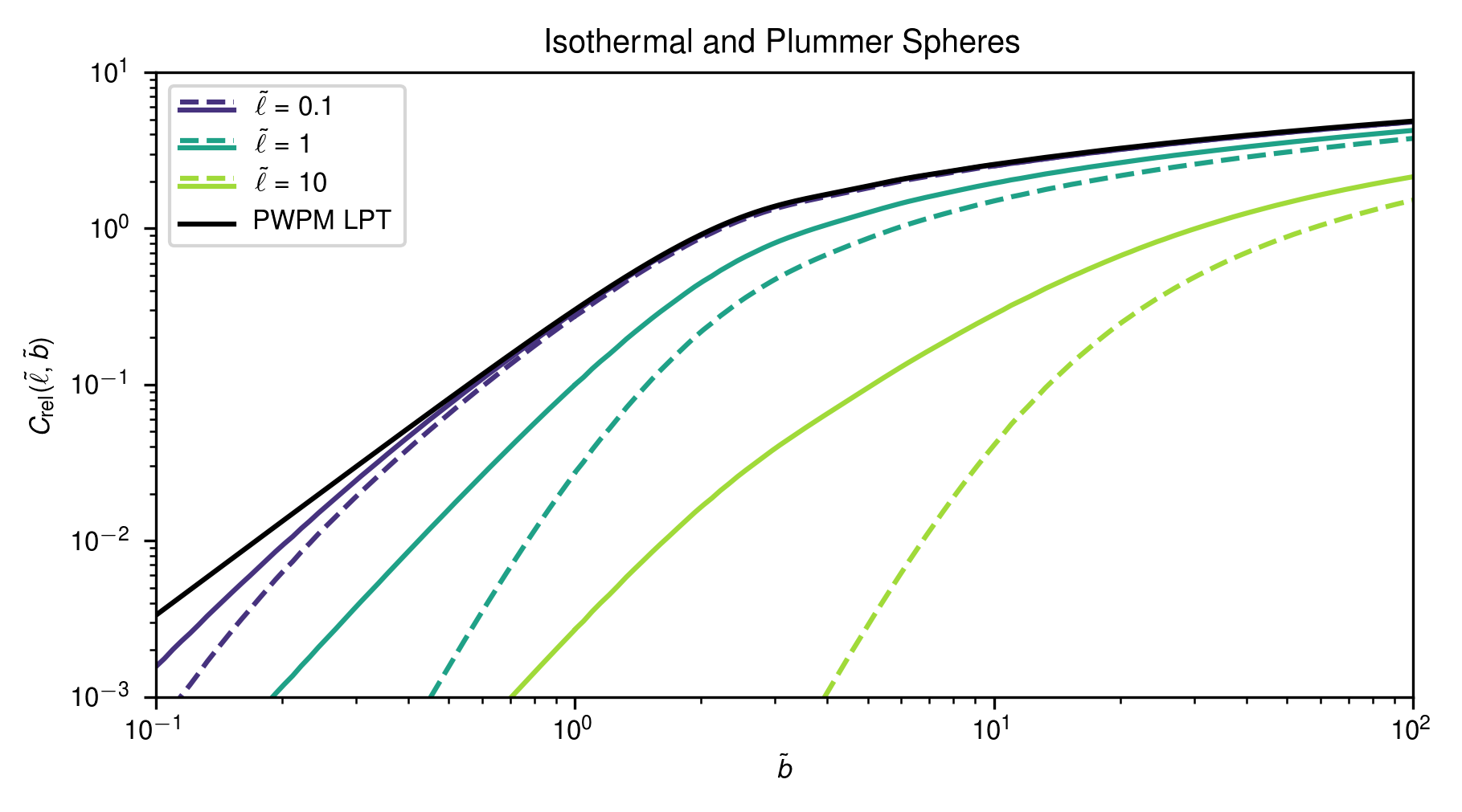
Figure 11: A comparison of the curves generated from plotting Eq. B.8 (shown in solid lines) and its analog for the case of a Plummer sphere (Eq. 4.31, shown in dashed lines) for three different satellite sizes, as a function of the dimensionless cutoff parameter $\tilde{b}$. The black line is the analagous curve for the perturbative solution in the case of a plane wave, point mass, linear perturbation theory (PWPM) solution. Note the qualitative similarities among all pairs of curves; where $b\gtrsim 100\ell$, the curves tend to agree for both the truncated isothermal and Plummer spheres, suggesting the dynamical friction is relatively insensitive to the matter distribution of the satellite in this regime.

The resulting curves from plotting Eq. B.8 are depicted in Fig. 11, alongside the analogous curves for the case of a Plummer sphere (Eq. 4.31) for comparison. Despite residing at opposite ends of the spectrum of profile densities, the curves are qualitatively very similar. This demonstrates that the dynamical friction from FDM is instead more sensitive to other parameters describing the satellite, such as its size, rather than the precise mass distribution within the satellite.

Appendix C Techniques for Numerical Simulations

Here, we outline the equations solved in our numerical simulations. The Schrödinger system is evolved with the unitary spectral method of [20]. Our code solves Eq. 4.1 with a Plummer profile satellite. The code solves the equations in dimensionless form, normalizing against the length-scale $L_{Q}$ (this is in contrast to normalization by ${\mkern 0.75mu\mathchar 22\relax\mkern-9.75mu\lambda}$ in the analytic calculations of the paper). We will indicate this by placing a breve ($\,\breve{\,}\,$) above dimensionless variables. Our dimensionless system of units for the simulation are:

$$\breve{x}\equiv\frac{x}{L_{\rm Q}}$$ (C.1)

$$\breve{t}\equiv\frac{t}{t_{\rm Q}}$$ (C.2)

$$\breve{\psi}\equiv\frac{\psi}{\sqrt{\overline{\rho}}},$$ (C.3)

where

$$t_{\rm Q}\equiv\frac{m}{\hbar}L_{\rm Q}^{2}$$ (C.4)

is the characteristic quantum-wave timescale. The satellite has dimensionless object size $\breve{\ell}=\ell/L_{\rm Q}$.

The Schrödinger equation thus becomes

$$i\frac{\partial}{\partial\breve{t}}\breve{\psi}=\left[-\frac{\breve{\nabla}^{2}}{2}-\frac{1}{\sqrt{\breve{r}^{2}+\breve{\ell}^{2}}}\right]\breve{\psi}$$ (C.5)

with initial condition:

$$\breve{\psi}_{0}=e^{i\mathcal{M}_{\rm Q}\breve{z}}.$$ (C.6)

The dimensionless satellite profile is:

$$\breve{\rho}_{\rm p}=\frac{3\breve{\ell}^{2}}{4\pi(\breve{\ell}^{2}+\breve{r}^{2})^{5/2}}\times\left(\frac{M_{\rm p}/L_{\rm Q}^{3}}{\overline{\rho}}\right).$$ (C.7)

The solution is updated via a second-order spectral method: each timestep can be broken into a half-step ‘kick’ from the potential, carried out in real space, followed by a full-step ‘drift’ from the kinetic operator carried out in Fourier space, followed by another half-step ‘kick’, as follows:

$$\breve{\psi}\leftarrow\exp\left[-i\frac{\Delta\breve{t}}{2}\times\frac{-1}{\sqrt{\breve{r}^{2}+\breve{\ell}^{2}}}\right]\breve{\psi}$$ (C.8)

$$\breve{\psi}\leftarrow{\rm ifft}\left[\exp\left[-i\Delta\breve{t}\times\breve{k}^{2}/2\right]{\rm fft}\left[\breve{\psi}\right]\right]$$ (C.9)

$$\breve{\psi}\leftarrow\exp\left[-i\frac{\Delta\breve{t}}{2}\frac{-1}{\sqrt{\breve{r}^{2}+\breve{\ell}^{2}}}\right]\breve{\psi}$$ (C.10)

where ${\rm fft}$ and ${\rm ifft}$ are numerical fast Fourier transform and inverse fast Fourier transform operations.

The drag coefficient can be calculated from the resulting acceleration field of the wavefuncion. The dimensionless acceleration field is:

$$\breve{\mathbf{a}}=-\nabla\breve{V}\cdot\left(\frac{4\pi G\overline{\rho}L_{\rm Q}^{4}m^{2}}{\hbar^{2}}\right),$$ (C.11)

where $\breve{V}$ is the dimensionless self-potential, $V\equiv\breve{V}\cdot(4\pi L_{\rm Q}^{2}G\overline{\rho})$, given by Poisson’s equation

$$\nabla^{2}\breve{V}=\left(|\breve{\psi}|^{2}-1\right).$$ (C.12)

This can be solved numerically in Fourier space:

$$\breve{V}={\rm ifft}\left[-{\rm fft}\left[\left(|\breve{\psi}|^{2}-1\right)\right]/\breve{k}^{2}\right].$$ (C.13)

Finally, the drag coefficient is

$$C_{\rm Q}=\frac{1}{4\pi}\int\breve{\rho}_{\rm p}\breve{a}_{\breve{z}}\,d\mathbf{\breve{x}}^{3}=-\int\frac{3\breve{\ell}^{2}\partial_{\breve{z}}\breve{V}}{4\pi(\breve{\ell}^{2}+\breve{r}^{2})^{5/2}}\,d\mathbf{\breve{x}}^{3}.$$ (C.14)

We carry out this integral numerically on the discretized domain.

Note that there is a general scaling symmetry of the equations:

$$\{x,t,\rho,m,M_{\rm p}\}\rightarrow\{ax,bt,c\rho,a^{-2}bm,a^{3}b^{-2}M_{\rm p}\}\,,$$ (C.15)

which can be used to transform our solutions to different satellite masses and FDM particle masses.

References

- [1] D. N. Spergel, L. Verde, H. V. Peiris, E. Komatsu, M. R. Nolta, C. L. Bennett et al., First-Year Wilkinson Microwave Anisotropy Probe (WMAP) Observations: Determination of Cosmological Parameters, ApJS 148 (2003) 175 [astro-ph/0302209].
- [2] Planck Collaboration, N. Aghanim, Y. Akrami, M. Ashdown, J. Aumont, C. Baccigalupi et al., Planck 2018 results. VI. Cosmological parameters, arXiv e-prints (2018) arXiv:1807.06209 [1807.06209].
- [3] S. Alam, M. Ata, S. Bailey, F. Beutler, D. Bizyaev, J. A. Blazek et al., The clustering of galaxies in the completed SDSS-III Baryon Oscillation Spectroscopic Survey: cosmological analysis of the DR12 galaxy sample, MNRAS 470 (2017) 2617 [1607.03155].
- [4] V. Springel, R. Pakmor, A. Pillepich, R. Weinberger, D. Nelson, L. Hernquist et al., First results from the IllustrisTNG simulations: matter and galaxy clustering, MNRAS 475 (2018) 676 [1707.03397].
- [5] L. Roszkowski, E. M. Sessolo and S. Trojanowski, WIMP dark matter candidates and searches–current status and future prospects, Reports on Progress in Physics 81 (2018) 066201 [1707.06277].
- [6] J. S. Bullock and M. Boylan-Kolchin, Small-Scale Challenges to the CDM Paradigm, Annual Review of Astronomy and Astrophysics 55 (2017) 343 [1707.04256].
- [7] A. Pontzen and F. Governato, How supernova feedback turns dark matter cusps into cores, MNRAS 421 (2012) 3464 [1106.0499].
- [8] J. I. Read, O. Agertz and M. L. M. Collins, Dark matter cores all the way down, MNRAS 459 (2016) 2573 [1508.04143].
- [9] A. Zolotov, A. M. Brooks, B. Willman, F. Governato, A. Pontzen, C. Christensen et al., Baryons Matter: Why Luminous Satellite Galaxies have Reduced Central Masses, ApJ 761 (2012) 71 [1207.0007].
- [10] A. R. Wetzel, P. F. Hopkins, J.-h. Kim, C.-A. Faucher-Giguère, D. Kereš and E. Quataert, Reconciling Dwarf Galaxies with CDM Cosmology: Simulating a Realistic Population of Satellites around a Milky Way-mass Galaxy, ApJ 827 (2016) L23 [1602.05957].
- [11] P. F. Hopkins, A. Wetzel, D. Kereš, C.-A. Faucher-Giguère, E. Quataert, M. Boylan-Kolchin et al., FIRE-2 simulations: physics versus numerics in galaxy formation, MNRAS 480 (2018) 800 [1702.06148].
- [12] A. A. Dutton, A. V. Macciò, J. Frings, L. Wang, G. S. Stinson, C. Penzo et al., NIHAO V: too big does not fail - reconciling the conflict between CDM predictions and the circular velocities of nearby field galaxies, MNRAS 457 (2016) L74 [1512.00453].
- [13] L. Hui, J. P. Ostriker, S. Tremaine and E. Witten, Ultralight scalars as cosmological dark matter, Phys. Rev. D 95 (2017) 043541 [1610.08297].
- [14] J. Goodman, Repulsive dark matter, New Astronomy 5 (2000) 103 [astro-ph/0003018].
- [15] W. Hu, R. Barkana and A. Gruzinov, Fuzzy Cold Dark Matter: The Wave Properties of Ultralight Particles, PRL 85 (2000) 1158 [astro-ph/0003365].
- [16] B. D. Wandelt, R. Dave, G. R. Farrar, P. C. McGuire, D. N. Spergel and P. J. Steinhardt, Self-Interacting Dark Matter, in Sources and Detection of Dark Matter and Dark Energy in the Universe (D. B. Cline, ed.), p. 263, Jan, 2001, astro-ph/0006344.
- [17] L. Berezhiani and J. Khoury, Theory of dark matter superfluidity, Phys. Rev. D 92 (2015) 103510 [1507.01019].
- [18] H.-Y. Schive, T. Chiueh and T. Broadhurst, Cosmic structure as the quantum interference of a coherent dark wave, Nature Physics 10 (2014) 496 [1406.6586].
- [19] H.-Y. Schive, M.-H. Liao, T.-P. Woo, S.-K. Wong, T. Chiueh, T. Broadhurst et al., Understanding the Core-Halo Relation of Quantum Wave Dark Matter from 3D Simulations, PRL 113 (2014) 261302 [1407.7762].
- [20] P. Mocz, M. Vogelsberger, V. H. Robles, J. Zavala, M. Boylan-Kolchin, A. Fialkov et al., Galaxy formation with BECDM - I. Turbulence and relaxation of idealized haloes, MNRAS 471 (2017) 4559 [1705.05845].
- [21] B. Bar-Or, J.-B. Fouvry and S. Tremaine, Relaxation in a Fuzzy Dark Matter Halo, ArXiv e-prints (2018) [1809.07673].
- [22] B. V. Church, P. Mocz and J. P. Ostriker, Heating of Milky Way disc stars by dark matter fluctuations in cold dark matter and fuzzy dark matter paradigms, MNRAS 485 (2019) 2861 [1809.04744].
- [23] P. Mocz, A. Fialkov, M. Vogelsberger, F. Becerra, M. A. Amin, S. Bose et al., First Star-Forming Structures in Fuzzy Cosmic Filaments, PRL 123 (2019) 141301 [1910.01653].
- [24] D. J. E. Marsh and J. Silk, A model for halo formation with axion mixed dark matter, MNRAS 437 (2014) 2652 [1307.1705].
- [25] S. D. Tremaine, J. P. Ostriker and J. Spitzer, L., The formation of the nuclei of galaxies. I. M31., ApJ 196 (1975) 407.
- [26] S. D. Tremaine, The formation of the nuclei of galaxies. II. The local group., ApJ 203 (1976) 345.
- [27] S. Tremaine and M. D. Weinberg, Dynamical friction in spherical systems., MNRAS 209 (1984) 729.
- [28] M. D. Weinberg, Evolution of barred galaxies by dynamical friction., MNRAS 213 (1985) 451.
- [29] M. C. Begelman, R. D. Blandford and M. J. Rees, Massive black hole binaries in active galactic nuclei, Nat 287 (1980) 307.
- [30] Q. Yu, Evolution of massive binary black holes, MNRAS 331 (2002) 935 [astro-ph/0109530].
- [31] L. Berezhiani, B. Elder and J. Khoury, Dynamical Friction in Superfluids, 1905.09297.
- [32] M. Safarzadeh and D. N. Spergel, Ultra-light Dark Matter is Incompatible with the Milky Way’s Dwarf Satellites, arXiv e-prints (2019) arXiv:1906.11848 [1906.11848].
- [33] S. Chandrasekhar, Dynamical Friction. I. General Considerations: the Coefficient of Dynamical Friction., ApJ 97 (1943) 255.
- [34] L. S. Marochnik, A Test Star in a Stellar System., jnlSoviet Ast. 11 (1968) 873.
- [35] A. J. Kalnajs, Polarization Clouds and Dynamical Friction, in IAU Colloq. 10: Gravitational N-Body Problem (M. Lecar, ed.), vol. 31 of Astrophysics and Space Science Library, p. 13, Jan, 1972, DOI.
- [36] E. C. Ostriker, Dynamical Friction in a Gaseous Medium, ApJ 513 (1999) 252 [astro-ph/9810324].
- [37] J. Binney and S. Tremaine, Galactic Dynamics: Second Edition. Princeton University Press, 2008.
- [38] M. D. Weinberg, Orbital Decay of Satellite Galaxies in Spherical Systems, ApJ 300 (1986) 93.
- [39] A. H. Guth, M. P. Hertzberg and C. Prescod-Weinstein, Do dark matter axions form a condensate with long-range correlation?, Phys. Rev. D 92 (2015) 103513 [1412.5930].
- [40] E. Madelung, Quantentheorie in hydrodynamischer Form, Zeitschrift fur Physik 40 (1927) 322.
- [41] L. M. Widrow and N. Kaiser, Using the Schroedinger Equation to Simulate Collisionless Matter, ApJ 416 (1993) L71.
- [42] P. Mocz, L. Lancaster, A. Fialkov, F. Becerra and P.-H. Chavanis, Schrödinger-Poisson-Vlasov-Poisson correspondence, Phys. Rev. D 97 (2018) 083519 [1801.03507].
- [43] X. Li, L. Hui and G. L. Bryan, Numerical and perturbative computations of the fuzzy dark matter model, Phys. Rev. D 99 (2019) 063509 [1810.01915].
- [44] V. Lora, J. Magaña, A. Bernal, F. J. Sánchez-Salcedo and E. K. Grebel, On the mass of ultra-light bosonic dark matter from galactic dynamics, JCAP 2 (2012) 011 [1110.2684].
- [45] E. Roetman, On the biharmonic wave equation, Pacific Journal of Mathematics 22 (1967) 139.
- [46] S. Timoshenko, History of strength of materials mcgraw-hill book company, Inc., New York/Toronto/London (1953) .
- [47] H. Bethe and E. Salpeter, Quantum Mechanics of One- and Two-Electron Atoms. Springer Berlin Heidelberg, 2013.
- [48] N. F. Mott and H. S. W. Massey, The theory of atomic collisions. Oxford University Press, 1949.
- [49] E. Yarnell Davies and P. Mocz, Fuzzy Dark Matter Soliton Cores around Supermassive Black Holes, arXiv e-prints (2019) arXiv:1908.04790 [1908.04790].
- [50] H. C. Plummer, On the problem of distribution in globular star clusters, MNRAS 71 (1911) 460.
- [51] J. F. Navarro, C. S. Frenk and S. D. M. White, A Universal Density Profile from Hierarchical Clustering, ApJ 490 (1997) 493 [astro-ph/9611107].
- [52] S. D. M. White and M. J. Rees, Core condensation in heavy halos: a two-stage theory for galaxy formation and clustering., MNRAS 183 (1978) 341.
- [53] J. W. Foster, N. L. Rodd and B. R. Safdi, Revealing the Dark Matter Halo with Axion Direct Detection, Phys. Rev. D97 (2018) 123006 [1711.10489].
- [54] M. G. Coleman and J. T. A. de Jong, A Deep Survey of the Fornax dSph. I. Star Formation History, ApJ 685 (2008) 933 [0805.1365].
- [55] E. Poretti, G. Clementini, E. V. Held, C. Greco, M. Mateo, L. Dell’Arciprete et al., Variable Stars in the Fornax dSph Galaxy. II. Pulsating Stars below the Horizontal Branch, ApJ 685 (2008) 947 [0806.4453].
- [56] S. S. Larsen, J. Strader and J. P. Brodie, Constraints on mass loss and self-enrichment scenarios for the globular clusters of the Fornax dSph, A&A 544 (2012) L14 [1207.5792].
- [57] D. R. Cole, W. Dehnen, J. I. Read and M. I. Wilkinson, The mass distribution of the Fornax dSph: constraints from its globular cluster distribution, MNRAS 426 (2012) 601 [1205.6327].
- [58] T. J. L. de Boer and M. Fraser, Four and one more: The formation history and total mass of globular clusters in the Fornax dSph, A&A 590 (2016) A35 [1510.05642].
- [59] A. del Pino, A. Aparicio, S. L. Hidalgo and E. L. Łokas, Rotating stellar populations in the Fornax dSph galaxy, MNRAS 465 (2017) 3708 [1605.09414].
- [60] J. I. Read, M. G. Walker and P. Steger, Dark matter heats up in dwarf galaxies, MNRAS 484 (2019) 1401 [1808.06634].
- [61] K. Kowalczyk, A. del Pino, E. L. Łokas and M. Valluri, Schwarzschild dynamical model of the Fornax dwarf spheroidal galaxy, MNRAS 482 (2019) 5241 [1807.07852].
- [62] P. Boldrini, R. Mohayaee and J. Silk, Does Fornax have a cored halo? Implications for the nature of dark matter, arXiv e-prints (2018) arXiv:1806.09591 [1806.09591].
- [63] M.-Y. Wang, T. de Boer, A. Pieres, T. S. Li, A. Drlica-Wagner, S. E. Koposov et al., The morphology and structure of stellar populations in the Fornax dwarf spheroidal galaxy from Dark Energy Survey Data, arXiv e-prints (2018) arXiv:1809.07801 [1809.07801].
- [64] M. Aaronson, Accurate radial velocities for carbon stars in Draco and Ursa Minor :the first hint of a dwarf spheroidal mass-to-light ratio., ApJ 266 (1983) L11.
- [65] M. L. Mateo, Dwarf Galaxies of the Local Group, Annual Review of Astronomy and Astrophysics 36 (1998) 435 [astro-ph/9810070].
- [66] G. Gilmore, M. Wilkinson, J. Kleyna, A. Koch, W. Evans, R. F. G. Wyse et al., Observed Properties of Dark Matter: dynamical studies of dSph galaxies, Nuclear Physics B Proceedings Supplements 173 (2007) 15 [astro-ph/0608528].
- [67] M. G. Walker and J. Peñarrubia, A Method for Measuring (Slopes of) the Mass Profiles of Dwarf Spheroidal Galaxies, ApJ 742 (2011) 20 [1108.2404].
- [68] M.-Y. Wang, S. Koposov, A. Drlica-Wagner, A. Pieres, T. Li, T. de Boer et al., Rediscovery of the Sixth Star Cluster in the Fornax Dwarf Spheroidal Galaxy, arXiv e-prints (2019) arXiv:1902.04589 [1902.04589].
- [69] X. Hernandez and G. Gilmore, Dynamical friction in dwarf galaxies, MNRAS 297 (1998) 517 [astro-ph/9802261].
- [70] K. S. Oh, D. N. C. Lin and H. B. Richer, Globular Clusters in the Fornax Dwarf Spheroidal Galaxy, ApJ 531 (2000) 727.
- [71] T. Goerdt, B. Moore, J. I. Read, J. Stadel and M. Zemp, Does the Fornax dwarf spheroidal have a central cusp or core?, MNRAS 368 (2006) 1073 [astro-ph/0601404].
- [72] M.-Y. Wang, T. de Boer, A. Pieres, T. S. Li, A. Drlica-Wagner, S. E. Koposov et al., The morphology and structure of stellar populations in the Fornax dwarf spheroidal galaxy from Dark Energy Survey Data, arXiv e-prints (2018) arXiv:1809.07801 [1809.07801].
- [73] A. del Pino, S. L. Hidalgo, A. Aparicio, C. Gallart, R. Carrera, M. Monelli et al., Spatial dependence of the star formation history in the central regions of the Fornax dwarf spheroidal galaxy, MNRAS 433 (2013) 1505 [1305.2166].
- [74] K. Kaur and S. Sridhar, Stalling of Globular Cluster Orbits in Dwarf Galaxies, ApJ 868 (2018) 134 [1810.00369].
- [75] A. D. Mackey and G. F. Gilmore, Surface brightness profiles and structural parameters for globular clusters in the Fornax and Sagittarius dwarf spheroidal galaxies, MNRAS 340 (2003) 175 [astro-ph/0211396].
- [76] M. Mateo, E. Olszewski, D. L. Welch, P. Fischer and W. Kunkel, A Kinematic Study of the Fornax Dwarf Spheroid Galaxy, AJ 102 (1991) 914.
- [77] M. G. Walker, M. Mateo, E. W. Olszewski, J. Peñarrubia, N. W. Evans and G. Gilmore, A Universal Mass Profile for Dwarf Spheroidal Galaxies?, ApJ 704 (2009) 1274 [0906.0341].
- [78] J. I. Read, M. G. Walker and P. Steger, Dark matter heats up in dwarf galaxies, MNRAS 484 (2019) 1401 [1808.06634].
- [79] R. A. Ibata, G. Gilmore and M. J. Irwin, A dwarf satellite galaxy in Sagittarius, Nat 370 (1994) 194.
- [80] K. V. Johnston, D. N. Spergel and L. Hernquist, The Disruption of the Sagittarius Dwarf Galaxy, ApJ 451 (1995) 598 [astro-ph/9502005].
- [81] A. Helmi, Velocity Trends in the Debris of Sagittarius and the Shape of the Dark Matter Halo of Our Galaxy, ApJ 610 (2004) L97 [astro-ph/0406396].
- [82] D. R. Law, K. V. Johnston and S. R. Majewski, A Two Micron All-Sky Survey View of the Sagittarius Dwarf Galaxy. IV. Modeling the Sagittarius Tidal Tails, ApJ 619 (2005) 807 [astro-ph/0407566].
- [83] V. Belokurov, D. B. Zucker, N. W. Evans, G. Gilmore, S. Vidrih, D. M. Bramich et al., The Field of Streams: Sagittarius and Its Siblings, ApJ 642 (2006) L137 [astro-ph/0605025].
- [84] D. R. Law and S. R. Majewski, The Sagittarius Dwarf Galaxy: A Model for Evolution in a Triaxial Milky Way Halo, ApJ 714 (2010) 229 [1003.1132].
- [85] C. W. Purcell, J. S. Bullock, E. J. Tollerud, M. Rocha and S. Chakrabarti, The Sagittarius impact as an architect of spirality and outer rings in the Milky Way, Nat 477 (2011) 301 [1109.2918].
- [86] S. E. Koposov, V. Belokurov, N. W. Evans, G. Gilmore, M. Gieles, M. J. Irwin et al., The Sagittarius Streams in the Southern Galactic Hemisphere, ApJ 750 (2012) 80 [1111.7042].
- [87] D. R. Law and S. R. Majewski, The Sagittarius Dwarf Tidal Stream(s), in Tidal Streams in the Local Group and Beyond (H. J. Newberg and J. L. Carlin, eds.), vol. 420, p. 31, Jan, 2016, DOI.
- [88] M. I. P. Dierickx and A. Loeb, Predicted Extension of the Sagittarius Stream to the Milky Way Virial Radius, ApJ 836 (2017) 92 [1611.00089].
- [89] N. Hernitschek, B. Sesar, H.-W. Rix, V. Belokurov, D. Martinez-Delgado, N. F. Martin et al., The Geometry of the Sagittarius Stream from Pan-STARRS1 3 RR Lyrae, ApJ 850 (2017) 96 [1710.09436].
- [90] M. A. Fardal, R. P. van der Marel, D. R. Law, S. T. Sohn, B. Sesar, N. Hernitschek et al., Connecting the Milky Way potential profile to the orbital time-scales and spatial structure of the Sagittarius Stream, MNRAS 483 (2019) 4724 [1804.04995].
- [91] I.-G. Jiang and J. Binney, The orbit and mass of the Sagittarius dwarf galaxy, MNRAS 314 (2000) 468 [astro-ph/9908025].
- [92] Gaia Collaboration, T. Prusti, J. H. J. de Bruijne, A. G. A. Brown, A. Vallenari, C. Babusiaux et al., The Gaia mission, A&A 595 (2016) A1 [1609.04153].
- [93] Gaia Collaboration, A. G. A. Brown, A. Vallenari, T. Prusti, J. H. J. de Bruijne, C. Babusiaux et al., Gaia Data Release 2. Summary of the contents and survey properties, A&A 616 (2018) A1.
- [94] S. A. Bird, X.-X. Xue, C. Liu, J. Shen, C. Flynn and C. Yang, Anisotropy of the Milky Way’s stellar halo using K giants from LAMOST and , ArXiv e-prints (2018) [1805.04503].
- [95] L. Lancaster, S. E. Koposov, V. Belokurov, N. W. Evans and A. J. Deason, The halo’s ancient metal-rich progenitor revealed with BHB stars, MNRAS 486 (2019) 378 [1807.04290].
- [96] G. Besla, N. Kallivayalil, L. Hernquist, B. Robertson, T. J. Cox, R. P. van der Marel et al., Are the Magellanic Clouds on Their First Passage about the Milky Way?, ApJ 668 (2007) 949 [astro-ph/0703196].
- [97] N. Kallivayalil, R. P. van der Marel, G. Besla, J. Anderson and C. Alcock, Third-epoch Magellanic Cloud Proper Motions. I. Hubble Space Telescope/WFC3 Data and Orbit Implications, ApJ 764 (2013) 161 [1301.0832].
- [98] D. Erkal, V. Belokurov, C. F. P. Laporte, S. E. Koposov, T. S. Li, C. J. Grillmair et al., The total mass of the Large Magellanic Cloud from its perturbation on the Orphan stream, MNRAS 487 (2019) 2685 [1812.08192].
- [99] N. Garavito-Camargo, G. Besla, C. F. P. Laporte, K. V. Johnston, F. A. Gómez and L. L. Watkins, Hunting for the Dark Matter Wake Induced by the Large Magellanic Cloud, arXiv e-prints (2019) arXiv:1902.05089 [1902.05089].
- [100] D. L. Nidever, K. Olsen, Y. Choi, T. J. L. de Boer, R. D. Blum, E. F. Bell et al., Exploring the Very Extended Low-surface-brightness Stellar Populations of the Large Magellanic Cloud with SMASH, ApJ 874 (2019) 118 [1805.02671].
- [101] Y. Choi, D. Nidever, K. Olsen, R. Blum, G. Besla and D. Zaritsky, SMASHing the LMC: A Tidally-induced Warp in the Outer LMC and a Large Scale Reddening Map, in American Astronomical Society Meeting Abstracts #233, vol. 233 of American Astronomical Society Meeting Abstracts, p. 416.06, Jan, 2019.
- [102] A. Khmelnitsky and V. Rubakov, Pulsar timing signal from ultralight scalar dark matter, JCAP 1402 (2014) 019 [1309.5888].
- [103] N. K. Porayko et al., Parkes Pulsar Timing Array constraints on ultralight scalar-field dark matter, Phys. Rev. D98 (2018) 102002 [1810.03227].
- [104] K. Watanabe, Integral transform techniques for Green’s function. Springer, 2014.