Asteroseismic constraints on the cosmic-time variation of
the gravitational constant from an ancient main-sequence star

Abstract

We investigate the variation of the gravitational constant $G$ over the history of the Universe by modeling the effects on the evolution and asteroseismology of the low-mass star KIC 7970740, which is one of the oldest ($\sim 11$ Gyr) and best-observed solar-like oscillators in the Galaxy. From these data we find ${\dot{G}/G=(1.2\pm 2.6)\times 10^{-12}~{}\text{yr}^{-1}}$, that is, no evidence for any variation in $G$. We also find a Bayesian asteroseismic estimate of the age of the Universe as well as astrophysical S-factors for five nuclear reactions obtained through a 12-dimensional stellar evolution Markov chain Monte Carlo simulation.

1 Introduction

Is the gravitational constant actually constant? Interest in this question goes back at least to the time of Dirac (1937). On the one hand, Einstein’s theory of general relativity says yes: according to the equivalence principle, the outcome of any local experiment in a freely falling laboratory is independent of its position in spacetime. Hence, $G$ is the same everywhere for all time. String theory and other theories of modified gravity, on the other hand, say no: the gravitational ‘constant’ is rather a derived parameter which can vary over cosmic time (see, e.g., Uzan 2003, 2011 and Chiba 2011 for reviews).

The constancy of $G$ is an empirical question which can be investigated through astrophysical experimentation. The strongest constraints to date come from the dynamics of the solar system. The Lunar Ranging Experiment (Smullin & Fiocco, 1962; Murphy, 2013) gives $\dot{G}/G={(7.1\pm 7.6)\times 10^{-14}}\;\text{yr}^{-1}$ over the past few decades (Hofmann & Müller, 2018). Similarly, the Messenger probe (Genova et al., 2018) has used the ephemeris of Mercury to find ${|\dot{G}|/G<4\times 10^{-14}}\;\text{yr}^{-1}$ over the past seven years. Other local (in both time and space) constraints have been derived from other planetary motions (Hellings et al., 1983), exoplanetary motions (Masuda & Suto, 2016), and pulsar binaries (Damour & Taylor, 1991; Zhu et al., 2019), among others.

Though these experiments are consistent with a constant $G$, they do not probe $\dot{G}$ over cosmic time, where presumably any major variations to $G$ would have transpired. Experiments which do probe cosmic time, albeit in a model-dependent fashion, include measurements from helioseismology (Guenther et al., 1998), white dwarfs (García-Berro et al., 2011; Córsico et al., 2013), and globular clusters (degl’Innocenti et al., 1996). More distant constraints have been derived from big bang nucleosynthesis (Accetta et al., 1990) and anisotropy in the cosmic microwave background (Nagata et al., 2004). These experiments are also consistent with a constant $G$, albeit with greater uncertainty ($|\dot{G}/G|\lessapprox 10^{-12}\;\text{yr}^{-1}$).

In this Letter, we contribute a new experiment to test the cosmic-time variation of $G$ using asteroseismology. Thanks to four years of observations from the Kepler mission (Borucki et al., 2010), there are now extraordinarily accurate measurements of stellar oscillations from solar-like stars in the Galaxy. For a typical well-observed solar-type star, dozens of oscillation mode frequencies can be resolved. As the properties of the oscillations depend on the properties of the star, asteroseismic data can be used to constrain stellar global parameters. By furthermore assuming that the theory of stellar evolution is approximately correct, constraints can be placed on the age and evolutionary history of the star by fitting models to the data.

Here we study a rich spectrum of acoustic oscillation mode frequencies measured from a low-mass solar-like star on the main sequence, KIC 7970740, and determine whether the observations of this star are consistent with a constant gravitational constant. The use of a low-mass star such as this one is ideal because it avoids the theoretical uncertainties associated with higher mass stars, such as element diffusion and convective core overshoot.

A variable gravitational constant has several consequences for stars and their evolution (e.g., Maeder, 1977). Teller (1948) showed that the luminosities of stars vary as $L\propto G^{7}M^{5}$; hence, ${\dot{G}\neq 0}$ directly changes the rate of stellar evolution (see Figure 2). Indeed, a negative $\dot{G}$ has been proposed as a resolution to the faint young Sun paradox (Sahni & Shtanov, 2014). This modification to stellar evolution then affects acoustic stellar oscillation mode frequencies and their associated separations and ratios (see Figure 2), as these quantities are sensitive to the composition of the stellar core.

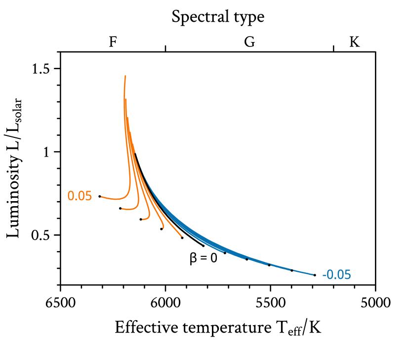
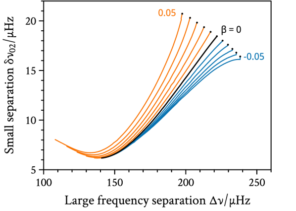
Figure 1: Theoretical evolution of a star with ${M/\text{M}_{\odot}=0.75}$ and ${Z=0.001}$ through the Hertzsprung–Russell diagram for varying amounts of ${\dot{G}}$ from the zero-age main sequence (black dots) until an age of 11 Gyr. Tracks computed with positive (negative) values of $\beta$ (cf. Equation 2) are shown in orange (blue), corresponding to gravity that was stronger (weaker) in the past.

Figure 2: The same as the previous figure, now showing the theoretical evolution of the star through the asteroseismic HR diagram (Christensen-Dalsgaard, 1988).

The star we have selected was observed in short-cadence mode (i.e., every 58.89 seconds) for nearly 3 years by Kepler. Its spectroscopic data and asteroseismic frequencies were measured by Lund et al. (2017), who identified 46 unique solar-like $p$-modes with spherical degrees ${\ell\leq 2}$. The extraordinary precision with which these measurements have been made are worthy of note: several of the modes have uncertainties smaller than 0.1 $\mu$Hz, corresponding to a relative uncertainty of approximately 0.001%. The global observable parameters of this star were measured to be:

$$\text{[Fe/H]}\;= ~{}-0.54 \pm 0.10~{}\text{dex}$$

$$T_{\text{eff}}\;= ~{}5309 \pm 77~{}\text{K}$$

$$\nu_{\max}\;= ~{}4197 \pm 20~{}\mu\text{Hz}$$ (1)

$$\Delta\nu\;= ~{}173.541 \pm 0.064~{}\mu\text{Hz}$$

$$\delta\nu_{02}\;= ~{}7.901 \pm 0.167~{}\mu\text{Hz}.$$

The first two of these are the stellar metallicity and effective temperature. The quantity $\nu_{\max}$ refers to the frequency at maximum oscillation power, which is related to the surface gravity of the star (e.g., Aerts et al., 2010; Basu & Chaplin, 2017). The average spacing between radial oscillation mode frequencies, i.e., the large frequency separation, is given by $\Delta\nu$, and is related to the stellar mean density. Finally, the small frequency separation—a proxy for the main-sequence age of the star—is denoted $\delta\nu_{02}$. From these measurements it is clear that this star is an old, low-mass star on the main sequence. This description has been confirmed through detailed numerical simulations of this star by several groups (Silva Aguirre et al., 2017; Creevey et al., 2017; Bellinger et al., 2019).

2 Methods

We aim to model KIC 7970740 with a time-varying gravitational constant, and determine the variations in $G$ which are empirically consistent with the stringent observational constraints that have been obtained for this star. As is commonly done (e.g., Demarque et al., 1994; Guenther et al., 1998; degl’Innocenti et al., 1996), we assume the gravitational constant $G$ varies over cosmic time $t$ according to a power law:

$$G(t)=G_{0}\left(\frac{t_{0}}{t}\right)^{\beta}$$ (2)

where ${G_{0}=(6.67408\pm 0.00031)\times 10^{-8}}$ g^-1 cm³ s^-2 is the presently observed gravitational constant (Mohr et al., 2016) and ${t_{0}=(13.799\pm 0.021)\times 10^{9}}$ yr is the current age of the Universe (Planck Collaboration et al., 2016). Here we seek to estimate the gravitational evolution parameter $\beta$, where a value of zero corresponds to a constant $G$.

We use the Aarhus STellar Evolution Code (ASTEC, Christensen-Dalsgaard, 2008a) to simulate the evolution of the star. We use the Aarhus adiabatic oscillation package (ADIPLS, Christensen-Dalsgaard, 2008b) to calculate the adiabatic oscillation mode frequencies for each of the computed models. Example evolutionary tracks were shown in Figures 2 and 2.

In order to determine which theoretical models are consistent with the observations, we use Markov chain Monte Carlo (MCMC, e.g., Goodman & Weare, 2010) to obtain 100 000 samples from the posterior distribution:

$$\underbrace{p(\boldsymbol{\theta}|\boldsymbol{D})}_{\text{posterior}}\propto\underbrace{\mathcal{L}(\boldsymbol{\theta}|\boldsymbol{D})}_{\text{likelihood}}\cdot\underbrace{p(\boldsymbol{\theta})}_{\text{prior}}.$$ (3)

Here the values ${\boldsymbol{\theta}=\{\beta},\tau,M,Y_{0},Z_{0},\alpha_{\text{MLT}},t_{0},\boldsymbol{S}(0)\}$ are the theoretical model parameters, where $\tau$ refers to the age of the star, $M$ its mass, $Y_{0}$ the initial fractional abundance of helium, $Z_{0}$ the initial fraction of heavy mass elements, $\alpha_{\text{MLT}}$ the mixing length parameter, and $\boldsymbol{S}(0)$ are astrophysical S-factors of nuclear reaction rates. We use uniform priors on the first six of these parameters as tabulated in Table 1. These priors were adopted because previous estimates for the parameters of this star came from the analysis of the same Kepler data, and thus normal priors would yield falsely overconfident results. We adopt a normal prior on the age of the Universe as given above as well as on the astrophysical S-factors as given in Table 2. The posterior distribution of $\dot{G}/G$, as reflected primarily in the distribution of $\beta$, is the main interest of the present work.

Table 1: Bounds on the Uniform Prior Distributions for the Input Parameters to the Stellar Evolution Simulations

Parameter	Minimum	Maximum	Unit
$\beta$	-0.2	0.2	–
$\tau$	0	$t_{0}$	Gyr
$M$	0.5	1	M⊙
$Y_{0}$	0.2	0.4	–
$Z_{0}$	0.001	0.02	–
$\alpha_{\text{MLT}}$	0.2	2.5	–

Table 2: Astrophysical S-factors of Nuclear Reactions

Reaction	$S(0)$/[keV b]
$p$($p$, e+ $\nu$)$d$	$4.01\,(1$	$\pm$	$0.01)\times 10^{-22}$
3He(3He, 2$p$)4He	$5.21\,(1$	$\pm$	$0.05)\times 10^{3}$
3He(4He, $\gamma$)7Be	$0.56\,(1$	$\pm$	$0.05)$
7Be($p$, $\gamma$)8B	$2.08\,(1$	$\pm$	$0.08)\times 10^{-2}$
14N($p$, $\gamma$)15O	$1.66\,(1$	$\pm$	$0.07)$

Note. All values obtained from Adelberger et al. 2011.

The values ${\boldsymbol{D}=\{T_{\text{eff}}},\text{[Fe/H]},\mathbf{r}_{102}\}$ are the observational data, the lattermost of which is a length-25 sequence comprised of $\mathbf{r}_{10}$ and $\mathbf{r}_{02}$ asteroseismic frequency separation ratios (Roxburgh & Vorontsov, 2003). These are defined as:

$$r_{10}(n) =\dfrac{\nu_{n-1,1}-4\nu_{n,0}+6\nu_{n,1}-4\nu_{n+1,0}+\nu_{n+1,1}}{\nu_{n,0}-8\nu_{n+1,0}}$$

$$r_{02}(n) =\dfrac{\nu_{n,0}-\nu_{n-1,2}}{\nu_{n,1}-\nu_{n-1,1}}$$ (4)

where $\nu_{n,\ell}$ refers to the frequency of the mode with radial order $n$ and spherical degree $\ell$. These quantities are useful because they probe the interior structure of the star and are insensitive to the near-surface layers.

The likelihood of the observed data for a given set of input parameters is given by

$$\mathcal{L}(\boldsymbol{\theta}|\boldsymbol{D})\propto\exp\left(-\frac{\chi^{2}}{2}\right)$$ (5)

where the goodness-of-fit $\chi^{2}$ in this case is

$$\chi^{2}=\mathbf{R}^{\text{T}}\boldsymbol{\Sigma}^{-1}\mathbf{R},\qquad R_{i}=D_{i}-A_{i}(\boldsymbol{\theta}).$$ (6)

Here $\mathbf{\Sigma}$ is the full variance–covariance matrix for the observations, which accounts for the fact the observed asteroseismic frequency ratios are correlated (Roxburgh, 2018); and $\mathbf{A}$ is the result of calling ASTEC and ADIPLS with the given model parameters $\boldsymbol{\theta}$. It is worthy of mention that previous MCMC asteroseismic modeling has considered at most a four-dimensional parameter space (see, e.g., Bazot et al., 2012; Lund & Reese, 2018; Rendle et al., 2019). With twelve dimensions, this is, to our knowledge, the most complex asteroseismic modeling performed to date.

3 Results & Conclusions

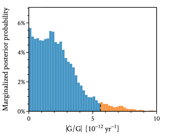
Figure 3: Histogram of MCMC samples showing the upper bound on the possible variation of $|\dot{G}/G|$. The 95% credible interval is in blue. Values closer to zero are in support of general relativity; values farther from zero are in support of modified gravity.

The procedure outlined in the previous section yields several results. The main result is the value of the gravitational evolution parameter, which we find to be ${\beta=0.017\pm 0.035}$. We also infer from this analysis an estimate of the age of the Universe, which we find to be ${t_{0}=13.797\pm 0.019}$ Gyr. Combining these two quantities yields a rate of change in $G$ of

$$\dot{G}/G=\beta/t_{0}=(1.2\pm 2.6)\times 10^{-12}~{}\text{yr}^{-1}.$$ (7)

Hence we find no evidence for a variable gravitational constant. We furthermore place a 95% upper bound on the absolute variation

$$|\dot{G}/G|\leq 5.6\times 10^{-12}\;\text{yr}^{-1}$$ (8)

as visualized in Figure 3. The posterior estimates for the five nuclear reaction rates are consistent with their prior values. We tested this procedure under two assumptions of the solar composition: the Grevesse & Sauval (1998, “GS98”) values and the Asplund et al. (2009, “AGSS09”) values, and found the results to be the same. These results are stronger than those from big bang nucleosynthesis, but probe less time; and weaker than those from helioseismology, but probe more than twice as much time.

Lastly, we obtain new estimates for the stellar parameters of KIC 7970740:

$$\tau\;= ~{}10.9 \pm 1.2~{}\text{Gyr}$$

$$M\;= ~{}0.725 \pm 0.043~{}\text{M}_{\odot}$$

$$Y_{0}\;= ~{}0.252 \pm 0.035$$ (9)

$$Z_{0}\;= ~{}0.0058 \pm 0.0012$$

$$\alpha_{\text{MLT}}\;= ~{}1.89 \pm 0.23.$$

These values are in good agreement with those presented by Silva Aguirre et al. (2017), who found for this star a mass of ${0.728\pm 0.020~{}\text{M}_{\odot}}$ and an age of $12.9\pm 1.6$ Gyr. It is worthy of note that the mean posterior value of the initial helium abundance of this star is above the primordial helium abundance $Y_{p}=0.2463$ inferred by the Planck mission (Coc et al., 2014).

Investigation into the constancy of G is still a very active area of inquiry spanning a wide range of domains in astrophysics. This work lays a bridge between asteroseismology and these other disciplines by enabling the use of individual stars for obtaining constraints at every age. In the future, it will be interesting to apply this technique to an ensemble of stars, which should yield an even stronger result. In addition, it will be interesting to use asteroseismology to constrain the variation of other values that are thought to be constant, such as the fine structure constant (Bonanno & Schlattl, 2006).

References

- Accetta et al. (1990) Accetta, F. S., Krauss, L. M., & Romanelli, P. 1990, Physics Letters B, 248, 146, doi: 10.1016/0370-2693(90)90029-6
- Adelberger et al. (2011) Adelberger, E. G., García, A., Robertson, R. G. H., et al. 2011, RMP, 83, 195, doi: 10.1103/RevModPhys.83.195
- Aerts et al. (2010) Aerts, C., Christensen-Dalsgaard, J., & Kurtz, D. W. 2010, Asteroseismology (Springer Science)
- Asplund et al. (2009) Asplund, M., Grevesse, N., Sauval, A. J., & Scott, P. 2009, ARA&A, 47, 481, doi: 10.1146/annurev.astro.46.060407.145222
- Basu & Chaplin (2017) Basu, S., & Chaplin, W. J. 2017, Asteroseismic Data Analysis (Princeton University Press). http://www.jstor.org/stable/j.ctt1vwmgmn
- Bazot et al. (2012) Bazot, M., Bourguignon, S., & Christensen-Dalsgaard, J. 2012, MNRAS, 427, 1847, doi: 10.1111/j.1365-2966.2012.21818.x
- Bellinger et al. (2019) Bellinger, E. P., Hekker, S., Angelou, G. C., Stokholm, A., & Basu, S. 2019, A&A, 622, arXiv:1812.06979, doi: 10.1051/0004-6361/201834461
- Bonanno & Schlattl (2006) Bonanno, A., & Schlattl, H. 2006, in ESA Special Publication, Vol. 617, SOHO-17, 37
- Borucki et al. (2010) Borucki, W. J., Koch, D., Basri, G., et al. 2010, Science, 327, 977, doi: 10.1126/science.1185402
- Chiba (2011) Chiba, T. 2011, Progress of Theoretical Physics, 126, 993, doi: 10.1143/PTP.126.993
- Christensen-Dalsgaard (1988) Christensen-Dalsgaard, J. 1988, in IAU Symposium, Vol. 123, Advances in Helio- and Asteroseismology, ed. J. Christensen-Dalsgaard & S. Frandsen, 295
- Christensen-Dalsgaard (2008a) Christensen-Dalsgaard, J. 2008a, Ap&SS, 316, 13, doi: 10.1007/s10509-007-9675-5
- Christensen-Dalsgaard (2008b) —. 2008b, Ap&SS, 316, 113, doi: 10.1007/s10509-007-9689-z
- Coc et al. (2014) Coc, A., Uzan, J.-P., & Vangioni, E. 2014, J. Cosmology Astropart. Phys, 2014, 050, doi: 10.1088/1475-7516/2014/10/050
- Córsico et al. (2013) Córsico, A. H., Althaus, L. G., García-Berro, E., & Romero, A. D. 2013, J. Cosmology Astropart. Phys, 6, 032, doi: 10.1088/1475-7516/2013/06/032
- Creevey et al. (2017) Creevey, O. L., Metcalfe, T. S., Schultheis, M., et al. 2017, A&A, 601, A67, doi: 10.1051/0004-6361/201629496
- Damour & Taylor (1991) Damour, T., & Taylor, J. H. 1991, ApJ, 366, 501, doi: 10.1086/169585
- degl’Innocenti et al. (1996) degl’Innocenti, S., Fiorentini, G., Raffelt, G. G., Ricci, B., & Weiss, A. 1996, A&A, 312, 345
- Demarque et al. (1994) Demarque, P., Krauss, L. M., Guenther, D. B., & Nydam, D. 1994, ApJ, 437, 870, doi: 10.1086/175048
- Dirac (1937) Dirac, P. A. M. 1937, Nature, 139, 323, doi: 10.1038/139323a0
- Foreman-Mackey et al. (2013) Foreman-Mackey, D., Hogg, D. W., Lang, D., & Goodman, J. 2013, PASP, 125, 306, doi: 10.1086/670067
- García-Berro et al. (2011) García-Berro, E., Lorén-Aguilar, P., Torres, S., Althaus, L. G., & Isern, J. 2011, J. Cosmology Astropart. Phys, 5, 021, doi: 10.1088/1475-7516/2011/05/021
- Genova et al. (2018) Genova, A., Mazarico, E., Goossens, S., et al. 2018, Nature Comm., 9, 289, doi: 10.1038/s41467-017-02558-1
- Goodman & Weare (2010) Goodman, J., & Weare, J. 2010, Comm. in Appl. Math. and Comp. Sci., 5, 65, doi: 10.2140/camcos.2010.5.65
- Grevesse & Sauval (1998) Grevesse, N., & Sauval, A. J. 1998, Space Sci. Rev., 85, 161, doi: 10.1023/A:1005161325181
- Guenther et al. (1998) Guenther, D. B., Krauss, L. M., & Demarque, P. 1998, ApJ, 498, 871, doi: 10.1086/305567
- Hellings et al. (1983) Hellings, R. W., Adams, P. J., Anderson, J. D., et al. 1983, Phys. Rev. Lett., 51, 1609, doi: 10.1103/PhysRevLett.51.1609
- Hofmann & Müller (2018) Hofmann, F., & Müller, J. 2018, Classical and Quantum Gravity, 35, 035015. http://stacks.iop.org/0264-9381/35/i=3/a=035015
- Lund & Reese (2018) Lund, M. N., & Reese, D. R. 2018, Asteroseismology and Exoplanets: Listening to the Stars and Searching for New Worlds, 49, 149, doi: 10.1007/978-3-319-59315-9_8
- Lund et al. (2017) Lund, M. N., Silva Aguirre, V., Davies, G. R., et al. 2017, ApJ, 835, 172, doi: 10.3847/1538-4357/835/2/172
- Maeder (1977) Maeder, A. 1977, A&A, 56, 359
- Masuda & Suto (2016) Masuda, K., & Suto, Y. 2016, PASJ, 68, L5, doi: 10.1093/pasj/psw017
- Mohr et al. (2016) Mohr, P. J., Newell, D. B., & Taylor, B. N. 2016, RMP, 88, 035009, doi: 10.1103/RevModPhys.88.035009
- Murphy (2013) Murphy, T. W. 2013, Reports on Progress in Physics, 76, 076901, doi: 10.1088/0034-4885/76/7/076901
- Nagata et al. (2004) Nagata, R., Chiba, T., & Sugiyama, N. 2004, Phys. Rev. D, 69, 083512, doi: 10.1103/PhysRevD.69.083512
- Planck Collaboration et al. (2016) Planck Collaboration, Ade, P. A. R., Aghanim, N., et al. 2016, A&A, 594, A13, doi: 10.1051/0004-6361/201525830
- R Core Team (2014) R Core Team. 2014, R, R Foundation. http://www.R-project.org/
- Rendle et al. (2019) Rendle, B. M., Buldgen, G., Miglio, A., et al. 2019, MNRAS, 484, 771, doi: 10.1093/mnras/stz031
- Roxburgh (2018) Roxburgh, I. W. 2018, arXiv e-prints. https://arxiv.org/abs/1808.07556
- Roxburgh & Vorontsov (2003) Roxburgh, I. W., & Vorontsov, S. V. 2003, A&A, 411, 215, doi: 10.1051/0004-6361:20031318
- Sahni & Shtanov (2014) Sahni, V., & Shtanov, Y. 2014, Int. J. Mod. Phys. D, 23, 1442018, doi: 10.1142/S0218271814420188
- Silva Aguirre et al. (2017) Silva Aguirre, V., Lund, M. N., Antia, H. M., et al. 2017, ApJ, 835, 173, doi: 10.3847/1538-4357/835/2/173
- Smullin & Fiocco (1962) Smullin, L. D., & Fiocco, G. 1962, Nature, 194, 1267, doi: 10.1038/1941267a0
- Teller (1948) Teller, E. 1948, Phys. Rev., 73, 801, doi: 10.1103/PhysRev.73.801
- Uzan (2003) Uzan, J.-P. 2003, RMP, 75, 403, doi: 10.1103/RevModPhys.75.403
- Uzan (2011) Uzan, J.-P. 2011, Living Reviews in Relativity, 14, 2, doi: 10.12942/lrr-2011-2
- Zhu et al. (2019) Zhu, W. W., Desvignes, G., Wex, N., et al. 2019, MNRAS, 482, 3249, doi: 10.1093/mnras/sty2905