Localizing Changes in High-Dimensional Vector Autoregressive Processes

Abstract

Autoregressive models capture stochastic processes in which past realizations determine the generative distribution of new data; they arise naturally in a variety of industrial, biomedical, and financial settings. A key challenge when working with such data is to determine when the underlying generative model has changed, as this can offer insights into distinct operating regimes of the underlying system. This paper describes a novel dynamic programming approach to localizing changes in high-dimensional autoregressive processes and associated error rates that improve upon the prior state of the art. When the model parameters are piecewise constant over time and the corresponding process is piecewise stable, the proposed dynamic programming algorithm consistently localizes change points even as the dimensionality, the sparsity of the coefficient matrices, the temporal spacing between two consecutive change points, and the magnitude of the difference of two consecutive coefficient matrices are allowed to vary with the sample size. Furthermore, the accuracy of initial, coarse change point localization estimates can be boosted via a computationally-efficient refinement algorithm that provably improves the localization error rate. Finally, a comprehensive simulation experiments and a real data analysis are provided to show the numerical superiority of our proposed methods.

Keywords: High dimensions; Vector autoregressive models; Dynamic programming; Change point detection.

1 Introduction

High-dimensional data are routinely collected in both traditional and emerging application areas. Time series data are by no means immune to this high dimensionality trend, and commonly arise in applications from econometrics (e.g. Bai and Perron, 1998; De Mol et al., 2008), finance (e.g. Chen and Gupta, 1997), genetics (e.g. Michailidis and d’Alché Buc, 2013), neuroimaging (e.g. Smith, 2012; Bolstad et al., 2011), predictive maintenance (e.g. Susto et al., 2014; Swanson, 2001; Yam et al., 2001), to name but a few.

Arguably, the most popular tool in modeling high-dimensional time series is the vector autoregressive (VAR) model (see e.g. Lütkepohl, 2005), where a $p$-dimension time series is at a given time is prescribed as white noise perturbation a linear combinations of its past values; see Section 1.1 below for a definition. In its simplest form, a VAR(1) model implies that $\mathbb{E}[X_{t+1}|X_{t}]=AX_{t}\in\mathbb{R}^{p}$ for $t\in\mathbb{Z}$ and a given $p\times p$ coefficient matrix $A$. When $p$ is large relative to the number of observed samples in the time series, we refer to this as a high-dimensional VAR model. A large body of literature focuses estimation of parameters of these processes when the time series is stationary (as detailed in the related work section). In this paper, we consider non-stationary VAR models in which the linear coefficients are allowed to change as a function time in piece-wise constant manner. For a VAR(1) model, this implies that

$$\mathbb{E}[X_{t+1}|X_{t}]=A_{t}X_{t}$$

where the entries of $A_{t}$ are piecewise-constant over time. The change point detection problem of interest is to estimate the times at which $A_{t+1}\neq A_{t}$. This model is defined precisely in 1 below.

Despite the vast body of literature on different change point detection problems, the study on 1 is scarce (e.g. Safikhani and Shojaie, 2020) and popular change point detection methods focusing on mean or covariance changes do not perform well when the data corresponds to a non-stationary VAR model. This claim is supported by extensive numerical experiments in Section 5.1; for now, we present a teaser in Example 1.

Example 1.

Let $\{X_{t}\}_{t=1}^{n}\in\mathbb{R}^{p}$ be generated from 1, with the number of samples $n=240$, $p=20$, lag $L=1$ and noise variance $\sigma^{2}_{\epsilon}=1$. The change points are $t=n/3$ and $t=2n/3$. The coefficient matrices are

$$A_{t}^{*}=\begin{cases}\left(v,-v,0_{p\times(p-2)}\right)\in\mathbb{R}^{p\times p},&t=1,\ldots,n/3-1,\\ \left(-v,v,0_{p\times(p-2)}\right)\in\mathbb{R}^{p\times p},&t=n/3,\ldots,2n/3-1,\\ \left(v,-v,0_{p\times(p-2)}\right)\in\mathbb{R}^{p\times p},&t=2n/3,\ldots,n,\end{cases}$$

where $v\in\mathbb{R}^{p}$ with odd coordinates being 0.1 and even coordinates being $-0.1$ and $0_{p\times(p-2)}\in\mathbb{R}^{p\times(p-2)}$ is an all zero matrix.

(A systematic study of Example 1 is provided in Section 5.1 scenario (ii).) Figures 1 and 2 show the first four coordinates of one realization of this process and the leading $4\times 4$ sub-matrices of their sample covariance matrices, respectively. As we can see from the black curves, the change points are not discernible from the raw data or the sample covariances. This phenomenon is further demonstrated in Figure 1 where two renowned competitors – “inspect” (Wang and Samworth, 2020) and “SBS-MVTS” (Baranowski and Fryzlewicz, 2019) – both fail here, but our proposed method penalized dynamic programming approach, indicated by DP and to be discussed in this paper, manages to identify the correct change points.

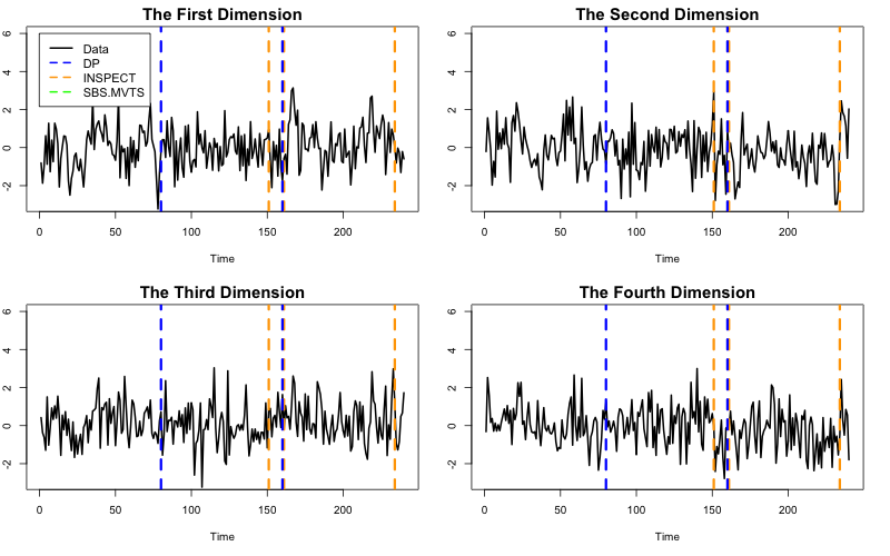
Figure 1: Example 1. Plots of the first four coordinates of a sample realization, $X_{t}[i]$ for $i=1,2,3,4$ as well as the results of three change point detection methods: DP (dynamic programming, this paper), INSPECT (Wang and Samworth, 2020), and SBS-MVTS (Baranowski and Fryzlewicz, 2019). Unlike the other two methods, the proposed DP approach correct identifies the change points at $t=80$ and $t=160$. These plots illustrate the difficulty of detecting changes in a VAR process by looking for changes in the mean. This example is detailed in Section 5.1.

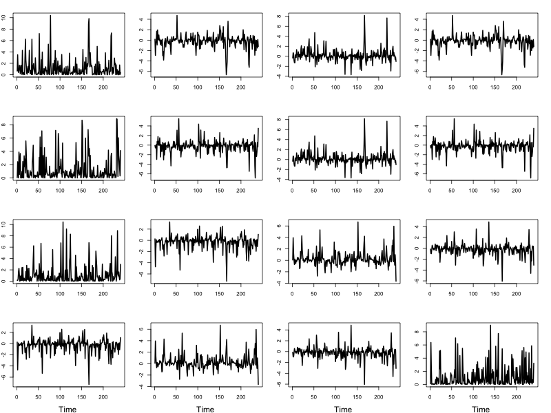
Figure 2: All sixteen coordinates of the leading $4\times 4$ sub-matrices of the sample covariance matrices of a realization from Example 1, $S_{t}[i,j]=X_{t}[i]X_{t}[j]$ for $i,j\in\{1,2,3,4\}$. These plots illustrate the difficulty of detecting changes in a VAR process by looking for changes in the covariance. This example is detailed in Section 5.1.

1.1 Problem formulation

We begin with a formal definition of a VAR process with lag $L$:

Definition 1 (Vector autoregressive process with lag $L$.).

The sequence $\{X_{t}\}_{t=-\infty}^{\infty}\subset\mathbb{R}^{p}$ is generated from a Gaussian vector autoregressive process with lag $L$, $L\geq 1$, if there exists a collection of coefficient matrices $A^{*}[1],\ldots,A^{*}[L]\in\mathbb{R}^{p\times p}$ such that

$$X_{t+1}=\sum_{l=1}^{L}A^{*}[l]X_{t+1-l}+\varepsilon_{t},\quad t\in\mathbb{Z},$$ (1)

where $\{\varepsilon_{t}\}_{t=-\infty}^{\infty}\stackrel{{\scriptstyle\mbox{i.i.d}}}{{\sim}}\mathcal{N}_{p}(0,\sigma_{\epsilon}^{2}I_{p})$ and $\sigma_{\epsilon}>0$.

In addition, the time series $\{X_{t}\}_{t=-\infty}^{\infty}\subset\mathbb{R}^{p}$ is stable, if

$$\det\left(I_{p}-\sum_{l=1}^{L}z^{l}A^{*}[l]\right)\neq 0,\quad\forall z\in\mathbb{C},\,|z|\leq 1.$$ (2)

In this paper, we study a specific type of non-stationary high-dimensional VAR model, which possesses piecewise-constant coefficient matrices, formally introduced in 1, which is built upon Definition 1.

Model 1 (Autoregressive model).

Let $(X_{1},\ldots,X_{n})$ be a time series with random vectors in $\mathbb{R}^{p}$ and let $1=\eta_{0}<\eta_{1}<\ldots<\eta_{K}\leq n<\eta_{K+1}=n+1$ be an increasing sequence of change points. Let $\Delta$ be the minimal spacing between consecutive change points, defined as

$$\Delta=\min_{k=1,\ldots,K+1}(\eta_{k}-\eta_{k-1}).$$ (3)

For any $k\in\{0,\ldots,K\}$, set $\mathcal{X}_{k}=\{X_{\eta_{k}},\ldots,X_{\eta_{k+1}-1}\}$. We assume the following.

• For each $k,l\in\{0,\ldots,K\}$, $k\neq l$, it holds that $\mathcal{X}_{k}$ and $\mathcal{X}_{l}$ are independent.

• For each $k\in\{0,\ldots,K\}$, $\mathcal{X}_{k}$ is a subset of an infinite stable time series $\mathcal{X}^{\infty}_{k}$ with coefficient matrices $\{A^{*}_{\eta_{k}}[l]\}_{l=1}^{L}$, with $1\leq L<\Delta$ (see Definition 1).

• For each $k\in\{0,\ldots,K\}$, $i\in\{0,\ldots,L-1\}$, $X_{\eta_{k}+i}$ satisfies the model

  $$X_{\eta_{k}+i}=\sum_{l=1}^{L}A_{\eta_{k}}^{*}[l]\widetilde{X}_{\eta_{k}+i-l}^{\top}+\varepsilon_{\eta_{k}+i},$$

  where $\widetilde{X}_{\eta_{k}+i-l}=X_{\eta_{k}+i-l}$ if $i-l\geq 0$, and $\widetilde{X}_{\eta_{k}+i-l}$’s are unobserved latent random vectors drawn from $\mathcal{X}^{\infty}_{k}$ if $i-l<0$.

Remark 1.

When defining a VAR($L$) process, one implicitly assumes the lag-$L$ coefficient matrix $A^{*}[L]$ is non-zero. In 1, we assume that each piece $\mathcal{X}_{k}$ is taken from a stable VAR($L$) process. In fact, what we only need is that $\mathcal{X}_{k}$ is taken from a stable VAR($L_{k}$) process and $L=\max_{k=0}^{K}L_{k}$.

Given data sampled from 1, our main task is to develop computationally-efficient algorithms that can consistently estimate both the unknown number $K$ of change points and the change points $\{\eta_{k}\}_{k=1}^{K}$, at which the coefficient matrices change. That is, we seek consistent estimators $\{\hat{\eta}_{k}\}_{k=1}^{\widehat{K}}$, such that, as the sample size $n$ grows unbounded, it holds with probability tending to 1 that

$$\widehat{K}=K\quad\mbox{and}\quad\frac{\epsilon}{\Delta}=\max_{k=1,\ldots,K}\frac{|\widehat{\eta}_{k}-\eta_{k}|}{\Delta}=o(1).$$

In the rest of the paper, we refer to $\epsilon$ as the localization error and $\epsilon/\Delta$ as the localization rate.

1.2 Summary of main contributions

We now summarize the main contributions of this paper. First, we provide accurate change point estimators for 1 in high-dimensional settings where we allow model parameters, including the dimensionality of the data $p$, the sparsity parameter $d_{0}$, defined to be the number of non-zero entries of the coefficient matrices, the number of change points $K$, the smallest distance between two consecutive change points $\Delta$, and the smallest difference between two consecutive different coefficient matrices $\kappa$ (formally defined in 9 below), to change with the sample size $n$. To the best of our knowledge, the theoretical results we provide in this paper are significantly sharper than any existing literature.

We note that these sharp bounds require several technical advances. Specifically, most existing change point detection methods assumes subsequent observations are independent, making key technical steps such as establishing restricted eigenvalue conditions easily verified. In contrast, our observations exhibit temporal dependence; no existing literature implies our results. Furthermore, we cannot directly leverage high-dimensional stationary VAR estimation bounds to obtain rates on change point detection. Analysis of our algorithm requires delicate treatment of small intervals between potential change points that allows us to prevent false discoveries and obtain sharp rates.

Second, we generalize the minimal partitioning problem (e.g. Friedrich et al., 2008) to suit the change point localizing problem in piecewise-stable high-dimensional vector autoregressive processes. The optimization problem can be solved using dynamic programming approaches in polynomial time. As we will further emphasize, this optimization tool is by no means new and has been mainly used to solve change point detection in univariate data sequences. In this paper, we have shown that for a much more sophisticated problem, this simple tool combined with the appropriate inputs computed by our method will still be able to produce consistent estimators.

Last, in the event that an initial estimator is at hand and satisfies mild conditions, we further devise an additional second step (Algorithm 2), to deliver a provably better localization error rate, even though our initial estimator’s output from the dynamic programming approach already provides the sharpest rates among the ones in the existing literature.

1.3 Related work

For the model described in Definition 1, if the dimensionality $p$ diverges as the sample size goes unbounded, then it is a high-dimensional VAR model, the recent literature on estimation of stationary high-dimensional VAR models is vast. Hsu et al. (2008), Haufe et al. (2010), Shojaie and Michailidis (2010), Basu and Michailidis (2015), Michailidis and d’Alché Buc (2013), Loh and Wainwright (2011), Wu and Wu (2016), Bolstad et al. (2011), Basu and Michailidis (2015), among many others, studied different aspects of the Lasso penalised VAR models; Han et al. (2015) utilized the Dantzig selector; Bickel and Gel (2011), Guo et al. (2016) and others resorted to banded autocovariance structures for time series modeling; the low rank conditions were exploited in Forni et al. (2005), Lam and Yao (2012), Chang et al. (2015), Chang et al. (2018), among many others; Xiao and Wu (2012), Chen et al. (2013) and Tank et al. (2015) focused on the properties of the covariance and precision matrices; various other inference related problems were also studied in Chang et al. (2017), Fiecas et al. (2018), Schneider-Luftman and Walden (2016), among many others.

The above list of references, far from being complete, is concerned with stationary time series. As for non-stationary high-dimensional time series data, Zhang et al. (2019) and Tu et al. (2017), among others, studied error-correction models; Wang et al. (2017) and Aue et al. (2009) examined the covariance change point detection problem; Cho and Fryzlewicz (2015),Cho (2016), Wang and Samworth (2018), Dette and Gösmann (2018), among many others, studied change point detection for high-dimensional time series with piecewise-constant mean; recently, Leonardi and Bühlmann (2016) examined the change point detection problem in regression setting and Safikhani and Shojaie (2020) proposed a fused-Lasso-based approach to estimate both the change points and the parameters of high-dimensional piecewise VAR models.

1.4 Notation

Throughout this paper, we adopt the following notation. For any set $S$, $|S|$ denotes its cardinality. For any vector $v$, let $\|v\|_{2}$, $\|v\|_{1}$, $\|v\|_{0}$ and $\|v\|_{\infty}$ be its $\ell_{2}$-, $\ell_{1}$-, $\ell_{0}$- and entry-wise maximum norms, respectively; and let $v(j)$ be the $j$th coordinate of $v$. For any square matrix $A\in\mathbb{R}^{n\times n}$, let $\Lambda_{\min}(A)$ and $\Lambda_{\max}(A)$ be the smallest and largest eigenvalues of matrix $A$, respectively; for a non-empty $S\subset\{1,\ldots,n\}$, let $A_{S}$ be the sub matrix of $A$ consisting of the entries in coordinates $S\times S$. For any matrix $B\in\mathbb{R}^{n\times m}$, let $\|B\|_{\text{op}}$ be the operator norm of $B$; let $\|B\|_{1}=\|\mathrm{vec}(B)\|_{1}$, $\|B\|_{2}=\|\mathrm{vec}(B)\|_{2}$ and $\|B\|_{0}=\|\mathrm{vec}(B)\|_{0}$, where $\mathrm{vec}(B)\in\mathbb{R}^{nm}$ is the vectorization of $B$ by stacking the columns of $B$. In fact, $\|B\|_{2}$ corresponds to the Frobenius norm of $B$. For any pair of integers $s,e\in\{0,1,\ldots,n\}$ with $s<e$, we let $(s,e]=\{s+1,\ldots,e\}$ and $[s,e]=\{s,\ldots,e\}$ be the corresponding integer intervals.

2 Methods

In this section, we detail our approaches. In Section 2.1, we use a dynamic programming approach to solve the minimal partition problem (4), which involves a loss function based on Lasso estimators of the coefficient matrices (6) and which provides a sequence of change point estimators. In Section 2.2, we propose an optional post-processing algorithm, which requires an initial estimate as input. Such inputs can (but is not restricted to) be the estimator analyzed in Section 2.1. The core of the post-processing algorithm is to exploit a group Lasso estimation to provide refined change point estimators.

2.1 The minimal partitioning problem and dynamic programming approach

To achieve the goal of obtaining consistent change point estimators, we adopt a dynamic programming approach. In detail, let $\mathcal{P}$ be an interval partition of $\{1,\ldots,n\}$ into $K_{\cal P}$ time intervals, i.e.

$$\mathcal{P}=\bigl{\{}\{1,\ldots,i_{1}-1\},\{i_{1},\ldots,i_{2}-1\},\ldots,\{i_{K_{\mathcal{P}}},\ldots,n\}\bigr{\}},$$

for some integers $1<i_{1}<\cdots<i_{K_{\mathcal{P}}}\leq n$, where $K_{\mathcal{P}}\geq 1$. For a positive tuning parameter $\gamma>0$, let

$$\widehat{\mathcal{P}}\in\operatorname*{arg\,min}_{\mathcal{P}}\left\{\sum_{I\in\mathcal{P}}\mathcal{L}(I)+\gamma|\mathcal{P}|\right\},$$ (4)

where $\mathcal{L}(\cdot)$ is a loss function to be specified below, $|\mathcal{P}|$ is the cardinality of $\mathcal{P}$ and the minimization is taken over all possible interval partitions of $\{1,\ldots,n+1\}$.

The change point estimator induced by the solution to (4) is simply obtained by taking all the left endpoints of the intervals $I\in\widehat{\mathcal{P}}$, except $1$. The optimization problem (4) is known as the minimal partition problem and can be solved using dynamic programming with computational cost of order $O\{n^{2}\mathcal{T}(n)\}$, where $\mathcal{T}(n)$ denotes the computational cost of solving $\mathcal{L}(I)$ with $|I|=n$ (see e.g. Algorithm 1 in Friedrich et al., 2008). Algorithms based on (4) are widely used in the change point detection literature. Friedrich et al. (2008), Killick et al. (2012), Rigaill (2010), Maidstone et al. (2017), Wang et al. (2018b), among others, studied dynamic programming approaches for change point analysis involving a univariate time series with piecewise-constant means. Leonardi and Bühlmann (2016) examined high-dimensional linear regression change point detection problems by using a version of dynamic programming approach.

We will tackle 1 in the framework of (4), by setting $I=[s,e]$, where $s>e$ are two positive integers and

$$\mathcal{L}(I)=\begin{cases}\sum_{t=s+L}^{e}\left\|X_{t}-\sum_{l=1}^{L}\widehat{A}_{I}[l]X_{t-l}\right\|^{2},&e-s-L+1\geq\gamma,\\ 0,&\text{otherwise,}\end{cases}$$ (5)

with

$$\left\{\widehat{A}_{I}[l]\right\}_{l=1}^{L}=\operatorname*{arg\,min}_{\{A[l]\}_{l=1}^{L}\in\mathbb{R}^{p\times p}}\sum_{t=s+L}^{e}\left\|X_{t}-\sum_{l=1}^{L}A[l]X_{t-l}\right\|^{2}+\lambda\sqrt{e-s-L+1}\sum_{l=1}^{L}\|A[l]\|_{1}.$$ (6)

In the sequel, for simplicity we refer to the change point estimation pipeline based on (4), (5) and (6) as the dynamic programming (DP) approach. In the DP approach, the estimation is twofold. Firstly, we estimate the high-dimensional coefficient matrices adopting the Lasso procedure in (6), where the tuning parameter $\lambda$ is used to obtain sparse estimates. Secondly, with the estimated coefficient matrices, we summon the minimal partitioning setup in (4) to obtain change point estimators, where the tuning parameter $\gamma$ is deployed to penalize over-partitioning. More discussions on the choice of tuning parameters will be provided later in the sense of both theoretical guarantees and practical guidance.

Note that in (5) and (6), the summation over $t$ is taken only from $s+L$ to $e$ in order to guarantee that the loss function $\mathcal{L}$ on each interval $I$ is solely depending on the information in that interval. For notational simplicity and with some abuse of the notation, in the proofs provided in the Appendices, we will just use $t\in I$ instead of $t\in[s+L,e]$.

For completeness, we present the DP procedure in Algorithm 1.

Data $\{X(t)\}_{t=1}^{n}$, tuning parameters $\lambda,\zeta>0$.

$(\mathcal{B},s,t,\mathrm{FLAG})\leftarrow(\emptyset,0,2,0)$

while $s<n-1$ do

     $s\leftarrow s+1$

     while $t<n$ and $\mathrm{FLAG}=0$ do

         $t\leftarrow t+1$ $\triangleright$ $\mathcal{L}(\cdot)$ is defined in (5)-(6) and $\lambda$ is involved thereof.

         if $\min_{l=s+1,\ldots,t-1}\{\mathcal{L}([s,l])+\mathcal{L}([l+1,t])+\gamma<\mathcal{L}([s,t])\}$ then

              $s\leftarrow\min\operatorname*{arg\,min}_{l=s+1,\ldots,t-1}\{\mathcal{L}([s,l])+\mathcal{L}([l+1,t])+\gamma<\mathcal{L}([s,t])\}$

              $\mathcal{B}\leftarrow\mathcal{B}\cup\{s\}$

              $\mathrm{FLAG}\leftarrow 1$

         end if

     end while

end while

The set of estimated change points $\mathcal{B}$.

Algorithm 1 Penalized dynamic programming. DP$(\{X(t)\}_{t=1}^{n},\lambda,\gamma)$

2.2 Post processing through group Lasso

As shown in Section 3 below, the DP approach in Algorithm 1 delivers consistent change point estimators with localization error rate that are sharper than any other rates previously established in the literature. In fact, these rates can be further improved upon by deploying a more sophisticated procedure that refines the initial change point estimators via post-processing through group Lasso (PGL), step detailed in Algorithm 2.

Data $\{X(t)\}_{t=1}^{n}$, a collection of time points $\{\widetilde{\eta}_{k}\}_{k=1}^{\widetilde{K}}$ , tuning parameter $\zeta>0$.

$(\widetilde{\eta}_{0},\widetilde{\eta}_{\widetilde{K}+1})\leftarrow(1,n+1)$

for $k=1,\ldots,\widetilde{K}$ do

     $(s_{k},e_{k})\leftarrow(2\widetilde{\eta}_{k-1}/3+\widetilde{\eta}_{k}/3,2\widetilde{\eta}_{k}/3+\widetilde{\eta}_{k+1}/3)$

     

$$\left(\widehat{A},\widehat{B},\widehat{\eta}_{k}\right)\leftarrow\operatorname*{arg\,min}_{\begin{subarray}{c}\eta\in\{s_{k}+L,\ldots,e_{k}-L\}\\ \{A[l]\}_{l=1}^{L},\{B[l]\}_{l=1}^{L}\subset\mathbb{R}^{p\times p}\end{subarray}}\Bigg{\{}\sum_{t=s_{k}+L}^{\eta}\bigl{\|}X_{t+1}-\sum_{l=1}^{L}A[l]X_{t+1-l}\bigr{\|}^{2}_{2}$$

$$+\sum_{t=\eta+L}^{e_{k}}\bigl{\|}X_{t+1}-\sum_{l=1}^{L}B[l]X_{t+1-l}\bigr{\|}_{2}^{2}+\zeta\sum_{l=1}^{L}\sum_{i,j=1}^{p}\sqrt{(\eta-s_{k})(A[l])_{ij}^{2}+(e_{k}-\eta)(B[l])_{ij}^{2}}\Bigg{\}}$$ (7)

end for

The set of estimated change points $\{\widehat{\eta}_{k}\}_{k=1}^{\widetilde{K}}$.

Algorithm 2 Post-processing through group Lasso. PGL$(\{X(t)\}_{t=1}^{n},\{\widetilde{\eta}_{k}\}_{k=1}^{\widetilde{K}},\zeta)$

The idea of the PGL algorithm is to refine a preliminary collection of change point estimators $\{\widetilde{\eta}_{k}\}_{k=1}^{K}$, which is taken in as inputs. The preliminary change point estimators produce a sequence of consecutive triplets $\{\widetilde{\eta}_{k},\widetilde{\eta}_{k+1},\widetilde{\eta}_{k+2}\}_{k=0}^{\widetilde{K}-1}$, with $\widetilde{\eta}_{k}=1$ and $\widetilde{\eta}_{K+1}=n+1$. The rest of the post processing works in each interval $(\widetilde{\eta}_{k},\widetilde{\eta}_{k+2})$ to refine the estimator $\widetilde{\eta}_{k+1}$, and thus can be scaled parallel.

In each interval, we first shrink it to a narrower one $(2\widetilde{\eta}_{k-1}/3+\widetilde{\eta}_{k}/3,2\widetilde{\eta}_{k}/3+\widetilde{\eta}_{k+1}/3)$, in order to avoid false positive. The constants $1/3$ and $2/3$ are to some extent ad hoc, but works for a wide range of initial estimators, which are not necessarily consistent. We then conduct group Lasso procedure stated in (7) to refine $\widetilde{\eta}_{k}$. The improvement will be quantified in Section 3. Intuitively, the group Lasso penalty exploits the piecewise-constant property of the coefficient matrices and improves the estimation. It is worth mentioning that one may replace the Lasso penalty in (6) with the group Lasso penalty in the initial estimation stage and to improve the estimation from there, but due to the computational cost of the group Lasso estimation, we stick to the two-step strategy we introduce in this paper.

3 Consistency of the change point estimators

In this section, we provide the theoretical guarantees for the change point estimators arising from the DP approach and the PGL algorithm, based on data generated from 1.

3.1 Assumptions

We begin by formulating the assumptions we impose to derive consistency guarantees.

Assumption 1.

Consider 1. We assume the following.

• (Sparsity). The coefficient matrices $\{A_{t}^{*}[l],\,l=1,\ldots,L\}$ satisfy the stability condition (2) and there exists a subset $S\subset\{1,\ldots,p\}^{\times 2}$, $|S|=d_{0}$, such that

  $$(A_{t}^{*}[l])(i,j)=0,\quad t=1,\ldots,n,\,l=1,\ldots,L,\,(i,j)\in S^{c}.$$

  In addition, suppose that

• (Spectral density conditions). For $k\in\{0,\ldots,K\}$, $h\in\mathbb{Z}$, let $\Sigma_{k}(h)$ be the population version of the lag-$h$ autocovariance function of $\mathcal{X}_{k}$ and let $f_{k}(\cdot)$ be the corresponding spectral density function, defined as

  $$\theta\in(-\pi,\pi]\mapsto f_{k}(\theta)=\frac{1}{2\pi}\sum_{\ell=-\infty}^{\infty}\Sigma_{k}(\ell)e^{-\imath\ell\theta}.$$

  Assume that

  $$\mathcal{M}=\max_{k=0,\ldots,K}\mathcal{M}(f_{k})=\max_{k=1,\ldots,K}\operatorname*{ess\,sup}_{\theta\in(-\pi,\pi]}\Lambda_{\max}(f_{k}(\theta))<\infty$$

  and

  $$\mathfrak{m}=\min_{k=0,\ldots,K}\mathfrak{m}(f_{k})=\min_{k=1,\ldots,K}\operatorname*{ess\,inf}_{\theta\in(-\pi,\pi]}\Lambda_{\min}(f_{k}(\theta))>0.$$

• (Signal-to-noise ratio). For any $\xi>0$, there exists an absolute constant $C_{\mathrm{SNR}}>0$, dependent on $\mathcal{M}$ and $\mathfrak{m}$, such that

  $$\Delta\kappa^{2}\geq C_{\mathrm{SNR}}d_{0}^{2}K\log^{1+\xi}(n\vee p),$$ (8)

  where $\Delta$ is the minimal spacing (see 3 above) and $\kappa$ is the minimal jump size, defined as

  $$\kappa=\min_{k=1,\ldots,K+1}\sqrt{\sum_{l=1}^{L}\|A^{*}_{\eta_{k}}[l]-A^{*}_{\eta_{k-1}}[l]\|^{2}_{2}}\quad\mbox{and}\quad\Delta=\min_{k=1,\ldots,K+1}(\eta_{k}-\eta_{k-1}).$$ (9)

  In addition, suppose that $0<\kappa<C_{\kappa}<\infty$ for some absolute constant $C_{\kappa}>0$.

1(a) and (b) are imposed to guarantee that the Lasso estimators in (6) exhibit good performance, while 1(c) can be interpreted as a signal-to-noise ratio condition for detecting and estimating the location of the change points. We further elaborate on these conditions next.

• Sparsity. The set $S$ appearing in 1(a) is a superset of the union of all the nonzero entries of all the coefficient matrices. If, alternatively, the sparsity parameter is defined as $d_{0}=\max_{t=1,\ldots,n}\left|S^{t}\right|$, where $S^{t}\subset\{1,\ldots,p\}^{\times 2}$ and $(A_{t}^{*}[l])(i,j)=0$, for all $(i,j)\in\{1,\ldots,p\}^{\times 2}\setminus S^{t}$, $l=1,\ldots,L$, then the signal-to-noise ratio in (8) and the localization error rate in Theorem 1 would change correspondingly, by replacing the sparsity level $d_{0}$ with $Kd_{0}$.

• Spectral Density. The spectral density condition in 1(b) is identical to Assumption 2.1 and the assumption in Proposition 3.1 in Basu and Michailidis (2015), which pertained to a stable VAR process without change points. As pointed out in Basu and Michailidis (2015), this holds for a large class of general linear processes, including stable ARMA processes.

• Signal-to-noise ratio. We assume $\kappa$ is upper bounded for stability, but we allow $\kappa\to 0$ as $n\to\infty$, which is more challenging in terms of detecting the change points. Since $\kappa<C_{\kappa}$, (8) also implies that

  $$\Delta\geq C^{\prime}_{\mathrm{SNR}}d_{0}^{2}K\log^{1+\xi}(n\vee p),$$

  where $C^{\prime}_{\mathrm{SNR}}=C_{\mathrm{SNR}}C_{\kappa}^{-2}$. For convenience, we will assume without loss of generality that $C_{\kappa}=1$.

  To facilitate the understanding of the signal-to-noise ratio condition, consider the case that $K=d_{0}=1$, (8) becomes

  $$\Delta\kappa^{2}\gtrsim\log^{1+\xi}(n\vee p),$$

  which matches be the minimax optimal signal-to-noise ratio (up to constants and logarithmic terms) for the univariate mean change point detection problem (see e.g. Chan and Walther, 2013; Frick et al., 2014; Wang et al., 2018b).

  1(c) can be expressed using a normalized jump size

  $$\kappa_{0}=\kappa/\sqrt{d_{0}},$$

  which leads to the equivalent signal-to-noise ratio condition

  $$\Delta\kappa_{0}^{2}\geq C_{\mathrm{SNR}}d_{0}K\log^{1+\xi}(n\vee p).$$

  Similar conditions are required in other change point detection problems, including high-dimensional mean change point detection (Wang and Samworth, 2018), high-dimensional covariance change point detection (Wang et al., 2017), sparse dynamic network change point detection (Wang et al., 2018a), high-dimensional regression change point detection (Wang et al., 2019), to name but a few. We remark that in these papers, which deploy variants of the wild binary segmentation procedure (Fryzlewicz, 2014), additional knowledge is needed in order to eliminate the dependence of the term $K$ in the signal-to-noise ratio condition. We refer the reader to Wang et al. (2018a) for more discussions regarding this point.

  The constant $\xi$ is needed to guarantee consistency and can be set to zero if $\Delta=o(n)$. We may instead replace it by a weaker condition of the form

  $$\Delta\kappa^{2}\gtrsim C_{\mathrm{SNR}}d_{0}^{2}K\{\log(n\vee p)+a_{n}\},$$

  where $a_{n}\to\infty$ arbitrarily slow as $n\to\infty$. We stick with the signal-to-noise ratio condition (8) for simplicity.

3.2 The consistency of the dynamic programming approach

In our first result, whose proof is given in Appendix A, we demonstrate consistency of the dynamic programming approach introduced in Section 2, under the assumptions listed in Section 3.1.

Theorem 1.

Assume 1 and let $L\in\mathbb{Z}^{+}$ be constant. Them, under 1, the change point estimators $\{\widehat{\eta}_{k}\}_{k=1}^{\widehat{K}}$ from the dynamic programming approach in Algorithm 1 with tuning parameters

$$\lambda=C_{\lambda}\sqrt{\log(n\vee p)}\quad\text{and}\quad\gamma=C_{\gamma}(K+1)d_{0}^{2}\log(n\vee p)$$ (10)

are such that

$$\mathbb{P}\left\{\widehat{K}=K\quad\mbox{and}\quad\max_{k=1,\ldots,K}|\widehat{\eta}_{k}-\eta_{k}|\leq\frac{KC_{\epsilon}d^{2}_{0}\log(n\vee p)}{\kappa^{2}}\right\}\geq 1-2(n\vee p)^{-1},$$

where $C_{\lambda},C_{\gamma},C_{\epsilon}>0$ are absolute constants depending only on $\mathcal{M}$, $\mathfrak{m}$ and $L$.

Remark 2.

We do not assume that Algorithm 1 admits a unique optimal solution $\widehat{\mathcal{P}}$. In fact the consistency result in Theorem 1 holds for any minimizer of DP.

Theorem 1 implies that with probability tending to 1 as $n$ grows,

$$\max_{k=1,\ldots,K}\frac{|\widehat{\eta}_{k}-\eta_{k}|}{\Delta}\leq\frac{KC_{\epsilon}d^{2}_{0}\log(n\vee p)}{\kappa^{2}\Delta}\leq\frac{C_{\epsilon}}{C_{\mathrm{SNR}}\log^{\xi}(n\vee p)}\to 0,$$

where the second inequality follows from 1(c). Thus, the localization error rate converges to zero in probability, yielding consistency.

The tuning parameter $\lambda$ affects the performance of the Lasso estimator, as elucidated in Lemma 12. The second tuning parameter $\gamma$ prevents overfitting while searching the optimal partition as a solution to the problem (4). In particular, $\gamma$ is determined by the squared $\ell_{2}$-loss of the Lasso estimator and is of order $\lambda^{2}d_{0}^{2}$.

We now compare the results in Theorem 1 with the guarantees established in Safikhani and Shojaie (2020).

• In terms of the localization error rate, Safikhani and Shojaie (2020) proved consistency of their methods by assuming that the minimal magnitude of the structural changes $\kappa$ is a sufficiently large constant independent of $n$, while our dynamic programming approach is valid even when $\kappa$ is allowed to decrease with the sample size $n$. In addition, Safikhani and Shojaie (2020) achieve the localization error bound of order

  $$K\widetilde{\Delta}d_{n}^{2},$$

  where $\widetilde{\Delta}$ satisfies $K^{2}d_{0}^{2}\log(p)\lesssim\widetilde{\Delta}\lesssim\Delta$. Translating to our notation, their best localization error is at least

  $$K^{5}d_{0}^{4}\log(p),$$

  which is larger than our rate $Kd_{0}^{2}\log(n\vee p)/\kappa^{2}$ even in their setting where $\kappa$ is a constant.

• In terms of methodology, Safikhani and Shojaie (2020) adopted a two-stage procedure: first, a penalized least squares estimator with a total variation penalty is deployed to obtain an initial estimator of the change points; then an information-type criterion is applied to identify the significant estimators and to remove any false discoveries. The change point estimators in Safikhani and Shojaie (2020) are selected from fused Lasso estimators, which are sub-optimal for change point detection purposes, especially when the size of the structure change $\kappa$ is small (see e.g. Lin et al., 2017). In addition, the theoretically-valid selection criterion proposed in Safikhani and Shojaie (2020) has a computational cost growing exponentially in $\widetilde{K}$, where $\widetilde{K}$ is the number of change points estimated by the fused Lasso and in general one has that $\widetilde{K}\gg K$.

3.3 The improvement of the post processing through group Lasso

We now show that the PGL refinement procedure (Algorithm 2) applied to the estimators $\{\widetilde{\eta}_{k}\}_{k=1}^{\widehat{K}}$ obtained wih Algorithm 1 delivers a smaller localization rate with no direct dependence on $K$.

Theorem 2.

Assume the same conditions in Theorem 1. Let $\{\widetilde{\eta}_{k}\}_{k=1}^{K}$ be any set of time points satisfying

$$\max_{k=1,\ldots,K}|\widetilde{\eta}_{k}-\eta_{k}|\leq\Delta/7.$$ (11)

Let $\{\widehat{\eta}_{k}\}_{k=1}^{K}$ be the change point estimators generated from Algorithm 2, with $\{\widetilde{\eta}_{k}\}_{k=1}^{K}$ and the tuning parameter

$$\zeta=C_{\zeta}\sqrt{\log(n\vee p)},$$

as inputs. Then

$$\mathbb{P}\left\{\max_{k=1,\ldots,K}|\hat{\eta}_{k}-\eta_{k}|\leq\frac{C_{\epsilon}d_{0}\log(n\vee p)}{\kappa^{2}}\right\}\geq 1-(n\vee p)^{-1},$$

where $C_{\zeta},C_{\epsilon}>0$ are absolute constants depending only on $\mathcal{M}$, $\mathfrak{m}$ and $L$.

As we have already shown in Theorem 1, the estimators of the change points obtained of DP detailed in Algorithm 1 satisfy, with high probability, condition (11) and therefore can serve as qualified inputs to Algorithm 2. However, we would like to emphasize that Theorem 2 holds even when the inputs are a sequence of inconsistent initial estimators of the change points.

Compared to the localization errors given in Theorem 1, the estimators refined by the PGL algorithm provide a substantial improvement by reducing the localization rate by a factor of $d_{0}K$. We provide some intuitive explanations for the success of the PGL algorithm.

• The intuition of the group Lasso penalty in (7) is as follows. Suppose that for simplicity $L=1$. The use of the penalty term

  $$\zeta\sum_{i,j=1}^{p}\sqrt{(\eta-s_{k})A_{ij}^{2}+(e_{k}-\eta)B_{ij}^{2}}$$

  implies that for any $(i,j)$th entry, the group lasso solution is such that either the $A_{ij}$’s’ and $B_{ij}$’s are simultaneously $0$ or they are simultaneously nonzero. This penalty effectively conforms to 1(a), which requires that all the population coefficient matrices share the common support.

• Even if the coefficient matrices do not share a common support, the group Lasso penalty (7) still works. Suppose again for simplicity that $L=1$. In addition, let $A^{*}_{t}$, $t\in[1,\eta_{1})$ have support $S_{1}$ and $A^{*}_{t}$, $t\in[\eta_{1},\eta_{2})$ have support $S_{2}\neq S_{1}$. Then the common support of $A_{t}^{*}$, $t\in[1,\eta_{2})$ is $S_{1}\cup S_{2}$. Since $|S_{1}\cup S_{2}|\leq 2d_{0}$, the localization rate in Theorem 2 will only be inflated by a constant factor. In fact, the numerical experiments in Section 5 also suggest that the PGL algorithm is robust even when the coefficient matrices do not share a common support.

• The condition (11) is to ensure that there is one and only one true change point in every working interval used by the local refinement algorithm. The true change points can then be estimated separately using $K$ independent searches, in such a way that the final localization rate does not depend on the number of searches.

4 Sketch of the proofs

In this section we provide a high-level summary of the technical arguments we use to prove Theorem 1 Theorem 2. The complete proofs are given in the Appendices. The main arguments consists of three main three steps. Firstly, we will express a VAR$(L)$ process with arbitrary but fixed lag $L$ into an appropriate VAR(1) process (this is a standard reduction technique). Then we will lay down the key ingredients needed to prove Theorem 1 and, lastly, we will pinpoint the main task to prove Theorem 2.

Transforming VAR($L$) processes to VAR(1) processes

For any general $L\in\mathbb{Z}^{+}$, a VAR($L$) process can be rewritten as a VAR(1) process in the following way. Assuming 1, let

$$Y_{t}=(\widetilde{X}_{t}^{\top},\ldots,\widetilde{X}_{t-L+1}^{\top})^{\top},$$ (12)

where, for $l\in\{0,\ldots,L-1\}$, $\widetilde{X}_{t-l}=X_{t-l}$ if $t-\max\{\eta_{k}:\,\eta_{k}\leq t\}\geq l$, and $\widetilde{X}_{t}$ is the unobserved random vector from drawn from $\mathcal{X}^{\infty}_{k}$, $k=\max\{j:\eta_{j}\leq t\}$ otherwise. In addition, let $\zeta_{t}=(\varepsilon_{t}^{\top},\ldots,\varepsilon_{t-L+1}^{\top})^{\top}$ and

$$\mathcal{A}^{*}_{t}=\left(\begin{array}[]{ccccc}A^{*}_{t}[1]&A^{*}_{t}[2]&\cdots&A^{*}_{t}[L-1]&A^{*}_{t}[L]\\ I&0&\cdots&0&0\\ 0&I&\cdots&0&0\\ \vdots&\vdots&\ddots&\vdots&\vdots\\ 0&0&\cdots&I&0\end{array}\right).$$ (13)

Then we can rewrite (1) as

$$Y_{t+1}=\mathcal{A}^{*}_{t}Y_{t}+\zeta_{t+1},$$ (14)

which is now a VAR(1) process. We remark that the stability condition (2) is now equivalent to all the eigenvalues of $\mathcal{A}^{*}_{t}$ as defined in (13) having a modulus strictly less than $1$ (e.g. Lütkepohl, 2005, Rule (7) in Section A.6 in). This further implies that (2) implies that $\|\mathcal{A}^{*}_{t}\|_{\mathrm{op}}\leq 1$.

The rest of the proof will be established based on this transformation, therefore, we assume $L=1$.

Sketch of the Proof of Theorem 1

Theorem 1 is an immediate consequence of the following Propositions 3 and 4.

Proposition 3.

Under all the conditions in Theorem 1, the following holds with probability at least $1-(n\vee p)^{-1}$.

• For each interval $\widehat{I}=(s,e]\in\widehat{\mathcal{P}}$ containing one and only one true change point $\eta$, it holds that

  $$\min\{e-\eta,\,\eta-s\}\leq C_{\epsilon}\left(\frac{d_{0}^{2}\lambda^{2}+\gamma}{\kappa^{2}}\right);$$

• for each interval $\widehat{I}=(s,e]\in\widehat{\mathcal{P}}$ containing exactly two true change points, say $\eta_{1}<\eta_{2}$, it holds that

  $$\max\{e-\eta_{2},\eta_{1}-s\}\leq C_{\epsilon}\left(\frac{d_{0}^{2}\lambda^{2}+\gamma}{\kappa^{2}}\right);$$

• for any two consecutive intervals $\widehat{I},\widehat{J}\in\widehat{\mathcal{P}}$, the interval $\widehat{I}\cup\widehat{J}$ contains at least one true change point; and

• no interval $\widehat{I}\in\widehat{\mathcal{P}}$ contains strictly more than two true change points.

The four cases in Proposition 3 are proved in Lemmas 5, 6, 7 and 8, respectively, and Proposition 3 is proved consequently.

Proposition 4.

Under the same conditions of Theorem 1, if $K\leq|\widehat{\mathcal{P}}|\leq 3K$, then with probability at least $1-(n\vee p)^{-1}$, it holds that $|\widehat{\mathcal{P}}|=K+1$.

Proof of Theorem 1.

It follows from Proposition 3 that, $K\leq|\widehat{\mathcal{P}}|-1\leq 3K$. This combined with Proposition 4 completes the proof. ∎

The key insight for the DP approach is that, for an appropriate value of $\lambda$, the estimator $\widehat{A}^{\lambda}_{I}$ in (6) based on any time interval $I$ is a “uniformly good enough” estimator, in the sense that it is sufficiently close to its population counterpart regardless of the choice of $I$ and even if $I$ contains multiple true change points. For instance, if $I$ contains three change points, then $I$ should not be a member in $\widehat{\mathcal{P}}$. This is guaranteed by the following arguments. Provided that $\widehat{A}^{\lambda}_{I}$ is close enough to its population counterpart, under the signal-to-noise ration condition in 1(c), breaking this interval $I$ will return a smaller objective function value in (4).

In order to show that $\widehat{A}^{\lambda}_{I}$ is a “good enough” estimator, we take advantage of the assumed sparsity of its population counterpart $A^{*}_{I}$ in Lemma 17. In particular, we show that $A^{*}_{I}$ is the unique solution to the equation

$$\left(\sum_{t\in I}\mathbb{E}[X_{t}X_{t}^{\top}]\right)(A_{I}^{*})^{\top}=\sum_{t\in I}\mathbb{E}[X_{t}X_{t}^{\top}](A_{t}^{*})^{\top}.$$

The above linear system implies that in general $A_{I}^{*}\not=|I|^{-1}\sum_{t\in I}A_{t}^{*}$, as the covariance matrix $\mathbb{E}[X_{t}X_{t}^{\top}]$ changes if $A_{t}^{*}$ changes at the change points. However, we can quantify the size of support of $A_{I}^{*}$ on any generic interval $I$ as long as $\{A_{t}^{*}\}_{t\in I}$ are sparse. With this at hand, we can further show that $\|\widehat{A}^{\lambda}_{I}-A^{*}_{I}\|^{2}_{2}=O_{p}(|I|^{-1})$, which is what makes $\widehat{A}^{\lambda}_{I}$ a “good enough” estimator for the purposes of change point localization.

The key ingredients of the proofs of both Propositions 3 and 4 are two types of deviation inequalities as follows.

• Restricted eigenvalues. In the literature on high-dimensional regression problems, there are several versions of the restricted eigenvalue conditions (see, e.g. Bühlmann and van de Geer, 2011). In our analysis, such conditions amount to controlling the probability of the event

  $$\left\{\|BX_{t}\|_{2}^{2}\geq\frac{|I|c_{x}}{4}\|B\|_{2}^{2}-C_{x}\log(p)\|B\|_{1}^{2},\quad\forall B\in\mathbb{R}^{p\times p},\,I\subset\{1,\ldots,n\}\right\}.$$

• Deviations bounds. In addition, we need to control the deviations of the quantities of the form

  $$\left\|\sum_{t\in I}\varepsilon_{t+1}X_{t}^{\top}\right\|_{\infty}$$

  for any interval $I\subset\{1,\ldots,n\}$.

Using well-established arguments to demonstrate the performance of the Lasso estimator, as detailed in e.g. Section 6.2 of Bühlmann and van de Geer (2011), the combination of restricted eigenvalues conditions and large probability bounds on the noise lead to oracle inequalities for the estimation and prediction errors in situations where there exists no change point and the data are independent. In the existing time series analysis literature, there are several versions of the aforementioned bounds for stationary VAR models (e.g. Basu and Michailidis, 2015). We have extended this line of arguments to the present, more challenging settings, to derive analogous oracle inequalities. See Appendix C for more details.

Sketch of the Proof of Theorem 2

The proof of Theorem 2 is based on an oracle inequality of the group Lasso estimator. Once it is established that for each interval $(s_{k},e_{k}]$ used in Algorithm 2,

$$\sum_{t=s_{k}}^{e_{k}}\|\widehat{A}_{t}-A^{*}_{t}\|_{2}^{2}\leq\delta\leq\kappa^{2}\Delta,$$ (15)

where $\delta\asymp d_{0}\log(n\vee p)$ and that there is one and only one change point in the interval $(s_{k},e_{k}]$ for both the sequence $\{\widehat{A}_{t}\}$ and $\{A^{*}_{t}\}$, then the final claim follows immediately that the refined localization error $\epsilon$ satisfies

$$\epsilon\leq\delta/\kappa^{2}.$$

The group Lasso penalty is deployed to prompt (15) and the designs of the algorithm guarantee the desirability of each working interval.

5 Numerical studies

In this section, we conduct a numerical study of the performance of the DP approach of Algorithm 1, of the PGL Algorithm 2 as well as some competing methods in a variety of different settings to support our theoretical findings. We will first provide numerical comparisons in the simulated data experiments then in a real data example. All the implementations of the numerical experiments can be found at https://github.com/darenwang/vardp.

We quantify the performance of the change point estimators $\{\widehat{\eta}_{k}\}_{k=1}^{\widehat{K}}$ relatively to the set $\{\eta_{k}\}_{k=1}^{K}$ of true change point using the absolute error $|\widehat{K}-K|$ and the scaled Hausdorff distance

$$\mathcal{D}(\{\widehat{\eta}_{k}\}_{k=1}^{\widehat{K}},\{\eta_{k}\}_{k=1}^{K})=\frac{d(\{\widehat{\eta}_{k}\}_{k=1}^{\widehat{K}},\{\eta_{k}\}_{k=1}^{K})}{n},$$

where $d(\cdot,\cdot)$ denotes the Hausdorff distance between two compacts sets in $\mathbb{R}$, given by

$$d(A,B)=\max\left\{\max_{a\in A}\min_{b\in B}|a-b|,\,\max_{b\in B}\min_{a\in A}|a-b|\right\}.$$

Note that if $\widehat{K},K\geq 1$, then $\mathcal{D}(\{\widehat{\eta}_{k}\}_{k=1}^{\widehat{K}},\{\eta_{k}\}_{k=1}^{K})\leq 1$. For convenience we set $\mathcal{D}(\emptyset,\{\eta_{k}\}_{k=1}^{K})=1$.

As discussed in Section 1, algorithms targeting at high-dimensional VAR change point detection are scarce. In addition, we cannot provide any numerical comparisons with Safikhani and Shojaie (2020), because their algorithm is NP-hard in the worst-case scenario. To be more precise, their combinatorial algorithm scales exponentially in $\widehat{K}$, which in general may be much bigger than $K$. In all the numerical experiments, we compare our methods with the SBS-MVTS procedure proposed in Cho and Fryzlewicz (2015) and the INSPECT method proposed in Wang and Samworth (2018). The SBS-MVTS is designed to detect covariance changes in VAR processes, and the INSPECT detects mean change points in high-dimensional sub-Gaussian vectors. We follow the default setup of the tuning parameters for the competitors, specified in the R (R Core Team, 2017) packages wbs (Baranowski and Fryzlewicz, 2019) and InspectChangepoint (Wang and Samworth, 2020), respectively.

For the tuning parameters used in our approaches, throughout this section, let $\lambda=0.1\sqrt{\log(p)}$, $\gamma=15\log(n)p$ and $\zeta=0.3\sqrt{\log(p)}$.

5.1 Simulations

We generate data according to 1 in three settings, each consisting of multiple setups, and for each setup we carry out 100 simulations. These three settings are designed to have varying minimal spacing $\Delta$, minimal jump size $\kappa$ and dimensionality $p$, respectively and are as follows:

• Varying $\Delta$. Let $n\in\{100,120,140,160\}$, $p=10$, $\sigma_{\epsilon}=1$ and $L=1$. The only change point occurs at $n/2$. The coefficient matrices are defined as

  $$A^{*}_{t}=\begin{cases}\begin{pmatrix}0.3&-0.3&&\\ &\ddots&\ddots&\\ &&0.3&-0.3\\ &&&0.3\end{pmatrix},&t\in\{1,\ldots,n/2-1\},\\ \begin{pmatrix}-0.3&0.3&&\\ &\ddots&\ddots&\\ &&-0.3&0.3\\ &&&-0.3\end{pmatrix},&t\in\{n/2,\ldots,n\},\end{cases}$$

  where the omitted entries that are zero.

• Varying $\kappa$. Let $n=240$, $p=20$, $\sigma_{\epsilon}=1$ and $L=1$. The change points occur at $n/3$ and $2n/3$. The coefficient matrices are

  $$A_{t}^{*}=\begin{cases}\rho(v,-v,0_{p-2}),&t\in\{1,\ldots,n/3-1\},\\ \rho(-v,v,0_{p-2}),&t\in\{n/3,\ldots,2n/3-1\},\\ \rho(v,-v,0_{p-2}),&t\in\{2n/3,\ldots,n\},\end{cases}$$ (16)

  where $v\in\mathbb{R}^{p}$ has odd coordinates equal 1 and even coordinates equal to $-1$, $0_{p-2}\in\mathbb{R}^{p\times(p-2)}$ is an all zero matrix and $\rho\in\{0.05,0.1,0.15,0.2,0.25\}$.

• Varying $p$. Let $T=240$, $p\in\{15,20,25,30,35\}$, $\sigma_{\epsilon}=1$ and $L=1$. The change points occur at $n/3$ and $2n/3$. The coefficient matrices are

  $$A_{t}^{*}=\begin{cases}(v_{1},v_{2},v_{3},0_{p-3}),&t\in\{1,\ldots,n/3-1\},\\ (v_{2},v_{3},v_{1},0_{p-3}),&t\in\{n/3,\ldots,2n/3-1\},\\ (v_{3},v_{2},v_{1},0_{p-3}),&t\in\{2n/3,\ldots,n\},\end{cases}$$

  where $v_{1},v_{2},v_{3}\in\mathbb{R}^{p}$ with

  $$v_{1}=(-0.15,0.225,0.25,-0.15,0,\ldots,0)^{\top},\quad v_{2}=(0.2,-0.075,-0.175,-0.05,0,\ldots,0)^{\top}$$

  and

  $$v_{3}=(-0.15,0.1,0.3,-0.05,0,\ldots,0)^{\top}.$$

Setting	Metric	PDP	PGL	SBS-MVTS	INSPECT
(i) n=100	$\mathcal{D}$	0.000 (0.000)	0.000 (0.000)	0.840 (0.348)	1.000 (0.000)
(i) n=120		0.000 (0.000)	0.000 (0.000)	0.600 (0.457)	0.989 (0.081)
(i) n=140		0.000 (0.000)	0.000 (0.000)	0.536 (0.470)	0.988 (0.082)
(i) n=160		0.000 (0.000)	0.000 (0.000)	0.367 (0.432)	0.995 (0.051)
(i) n=100	$|\widehat{K}-K|$	0.000 (0.000)	0.000 (0.000)	0.820 (0.386)	1.000 (0.000)
(i) n=120		0.000 (0.000)	0.000 (0.000)	0.560 (0.499)	0.980 (0.141)
(i) n=140		0.000 (0.000)	0.000 (0.000)	0.500 (0.502)	0.990 (0.100)
(i) n=160		0.000 (0.000)	0.000 (0.000)	0.310 (0.465)	0.990 (0.100)
(ii) $\rho=0.05$	$\mathcal{D}$	0.049 (0.026)	0.041 (0.030)	0.990 (0.076)	1.000 (0.000)
(ii) $\rho=0.10$		0.035(0.027)	0.022 (0.027)	0.994 (0.059)	1.000 (0.000)
(ii) $\rho=0.15$		0.022 (0.024)	0.009 (0.017)	1.000 (0.000)	0.996 (0.043)
(ii) $\rho=0.20$		0.010 (0.018)	0.004 (0.012)	0.995 (0.054)	0.955 (0.147)
(ii) $\rho=0.25$		0.004 (0.013)	0.002 (0.009)	1.000 (0.000)	0.831 (0.260)
(ii) $\rho=0.05$	$|\widehat{K}-K|$	0.000 (0.000)	0.000 (0.000)	1.980 (0.140)	2.000 (0.000)
(ii) $\rho=0.10$		0.000 (0.000)	0.000 (0.000)	1.990 (0.100)	2.000 (0.000)
(ii) $\rho=0.15$		0.000 (0.000)	0.000 (0.000)	2.000 (0.000)	1.999 (0.100)
(ii) $\rho=0.20$		0.000 (0.000)	0.000 (0.000)	1.990 (0.100)	1.890 (0.373)
(ii) $\rho=0.25$		0.000 (0.000)	0.000 (0.000)	2.000 (0.000)	1.650 (0.575)
(iii) $p=15$	$\mathcal{D}$	0.049 (0.034)	0.026 (0.031)	1.000 (0.000)	1.000(0.000)
(iii) $p=20$		0.059 (0.031)	0.036 (0.032)	1.000 (0.000)	1.000 (0.000)
(iii) $p=25$		0.057 (0.028)	0.034 (0.029)	1.000 (0.000)	0.992(0.073)
(iii) $p=30$		0.058 (0.028)	0.027 (0.030)	1.000 (0.000)	1.000 (0.000)
(iii) $p=35$		0.043 (0.024)	0.026 (0.031)	0.986 (0.097)	0.987 (0.092)
(iii) $p=15$	$|\widehat{K}-K|$	0.000 (0.000)	0.000 (0.000)	2.000 (0.000)	2.000 (0.000)
(iii) $p=20$		0.000 (0.000)	0.000 (0.000)	2.000 (0.000)	2.000 (0.000)
(iii) $p=25$		0.000 (0.000)	0.000 (0.000)	2.000 (0.000)	1.990 (0.100)
(iii) $p=30$		0.000 (0.000)	0.000 (0.000)	2.000 (0.000)	2.000 (0.000)
(iii) $p=35$		0.000 (0.000)	0.000 (0.000)	1.980 (0.141)	1.980 (0.141)

Table 1: Simulation results. Each cell is based on 100 repetitions and is in the form of mean(standard error).

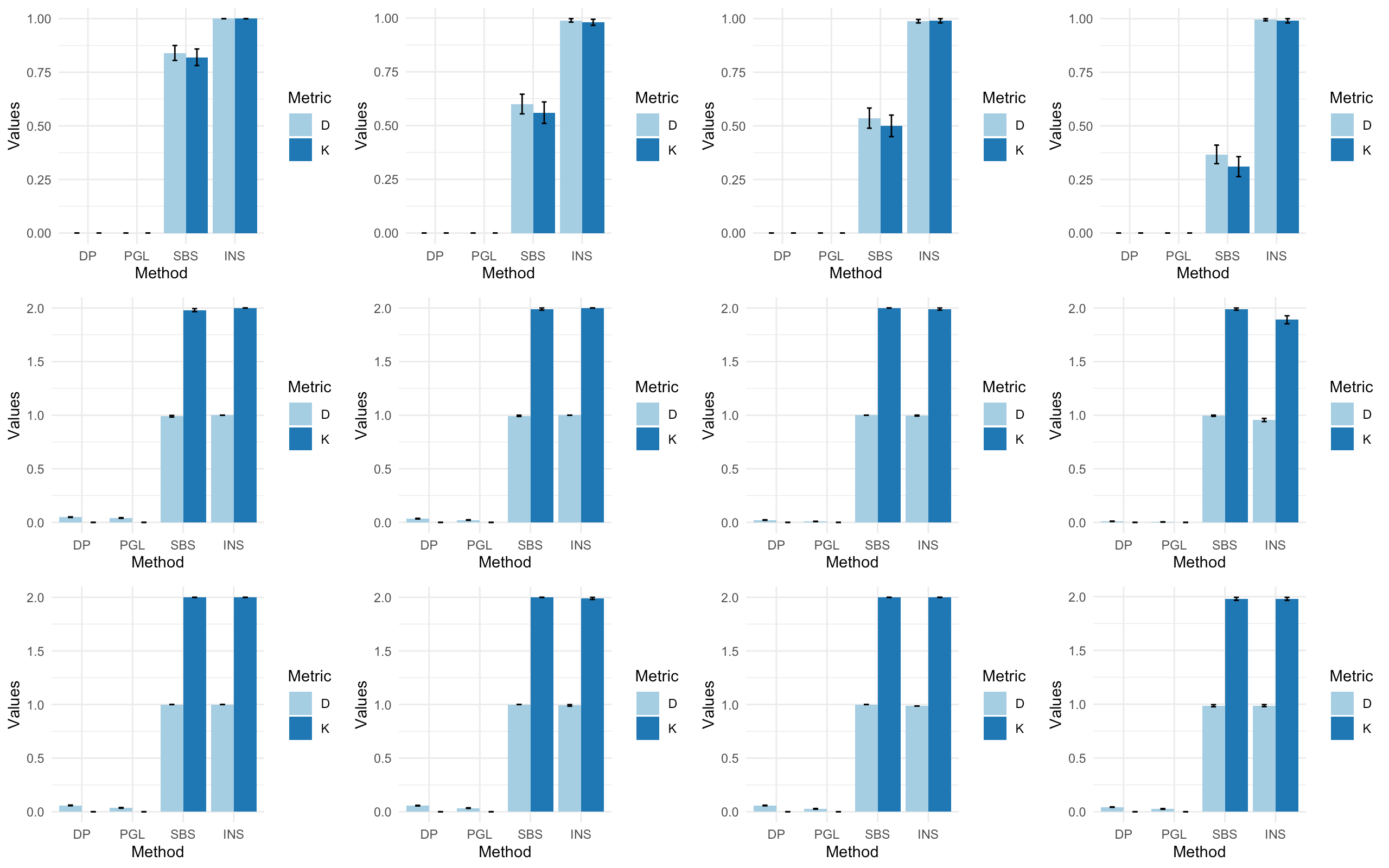
Figure 3: Bar plots visualizing the results collected in Table 1. From left to right and from top to bottom are Setting (i) with $n\in\{100,120,140,160\}$, Setting (ii) with $\rho\in\{0.05,0.1,0.15,0.2\}$ and Setting (iii) with $p\in\{20,25,30,35\}$, respectively. The four methods are: DP, Algorithm 1; PGL, Algorithm 2, SBS, SBS-MVTS; INS, Inspect. The two metrics are: D, $\mathcal{D}$; K, $|\widehat{K}-K|$.

The numerical comparisons of all algorithms in terms of the absolute error $|\widehat{K}-K|$ and the scaled Hausdorff distance $\mathcal{D}$ are reported in Table 1 and are also displayed in Figure 3. We can see that even though the dimension $p$ is moderate, neither SBS-MVTS nor INSPECT can consistently estimate the change points. In fact, both algorithms tend to infer that there is no change points in the time series, confirming the intuition discussed in Example 1.

In all of our approaches, we need to estimate the coefficient matrices, therefore the effective dimensions are $p^{2}$, but not $p$. The competitors SBS-MVTS and INSPECT, however, estimate the change points without estimating the coefficient matrices. This reduces the effective dimension to $p$, which might be more efficient in terms of computation, but neither SBS-MVTS nor INSPECT can consistently estimate the change points in these settings.

5.2 A real data example: S&P 100

We study the daily closing prices of the constituents of S&P 100 index from Jan 2016 to Oct 2018. The companies in the S&P 100 are selected for sector balance and represent about 51% of the market capitalization of the U.S. equity market. They tend to be the largest and most established firms in the U.S. stock market. Since the stock prices always exhibit upward trends, we therefore follow the standard procedure and de-trend the data by taking the first order difference. After removing missing values, our final dataset is a multivariate time series with $n=700$ and $p=93$, where each dimension corresponds the daily stock price change of one firm during the aforementioned period.

In order to apply our algorithms, we rescale the data so that the average variance over all dimensions equals 1. We apply the DP and PGL algorithms to the data set and depict the detected change points in Figure 4a. Since the outputs of these two algorithms do not differ by much, we focus on the ones output by DP. The five estimated change points by DP are 3rd November 2016, 23rd March 2017, 15th August 2017, 29th December 2017 and 10th May 2018. There are some times, e.g. around Feb. 2018, where we see big changes in the S&P 100 index but none of the methods describes it as a change point. This is because our change point analysis is targeting changes in the interactions among companies, as captured by a VAR process, and not directly the mean price changes. Thus occasional large fluctuations in the data do not necessarily reflect the type of structural changes we seek to identify.

To argue that our methodology has lead to meaningful findings, we suggest a justification of each estimated change points. Four days after the first change point estimator, Trump won the presidential election. Eight days after the second change point estimator, President Trump signed two executive orders increasing tariffs. This is a key date in the U.S.-China trade war. The third change point estimator is associated with President Trump signing another executive order in March 2017, authorizing U.S. Trade Representatives to begin investigations into Chinese trade practices, with particular focus on intellectual property and advanced technology. The fourth change point estimator lines up with the best opening of the U.S. stock market in 31 years (e.g. Franck, 2018). The last change point estimator is associated with the White House announcement that it would impose a 25% tariff on $50 billion of Chinese goods with industrially significant technology at the end of May 2018. For comparison, we also show the change points found by SBS-MVTS and INSPECT in Figure 4b.

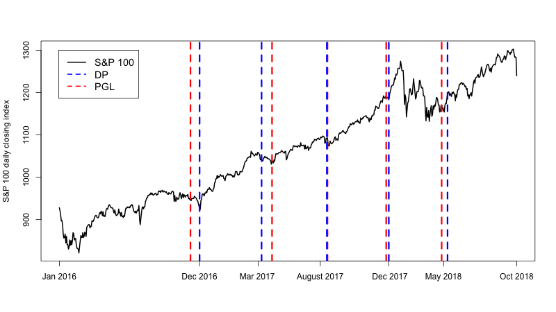
(a)

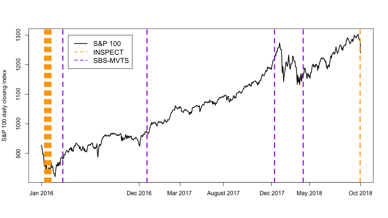
(b)

Figure 4: S&P 100 example. (a) Change points estimated by the DP and PGL algorithms. (b) Change points estimated by SBS-MVTS and INSPECT algorithms. While the plot is only showing the daily closing index, our method is using the first order difference of $p=93$ stocks that comprise the index. All the change point algorithms analyzed in this section focus on the interactions among those 93 companies, not in changes in the S&P 100 stock index.

6 Conclusions

This paper considers change point localization in high-dimensional vector autoregressive process models. We have developed two procedures for change point localization that can be characterized as solutions to a common optimization framework and that can be efficiently implemented using a combination of dynamic programming and Lasso-type estimators. We have demonstrated that our methods yield the sharpest localization rates of autoregressive processes and match the best known rates for change point localization. We further conjecture that the localization rate of the PGL algorithm is minimax optimal. Both minimax rates and extensions of this framework beyond sparse models to other models of low-dimensional structure remain important open questions for future research.

Appendix

In the proofs, we do not track every single absolute constant. Except those which have specific meanings, used in the main text, all the others share a few pieces of notation, i.e. the constant $C$ are used in different places having different values.

Appendix A Proof of Theorem 1

As we mentioned in Section 4, for any positive integer $L$, a VAR($L$) process can be written as a VAR(1) process. Based on the transformation introduced in Section 4, in this section, we will first lay down the preparations, then prove Propositions 3 and 4 based on $L=1$. All the technical lemmas are deferred to Appendix C.

We let $A_{I}^{*}$ be the solution to

$$\left(\sum_{t\in I}\mathbb{E}(X_{t}X_{t}^{\top})\right)(A_{I}^{*})^{\top}=\sum_{t\in I}\mathbb{E}(X_{t}X_{t}^{\top})(A_{t}^{*})^{\top}.$$ (17)

Note that when $I$ contains no change points $A_{I}^{*}=A_{t}^{*}$, $t\in I$. Let

$$S_{1}=\{i:\,(i,j)\in S\}\subset\{1,\ldots,p\}\quad\mbox{and}\quad S_{2}=\{j:\,(i,j)\in S\}\subset\{1,\ldots,p\}.$$

Therefore by 1(a), $\max\{|S_{1}|,\,|S_{2}|\}\leq d_{0}$. With a permutation if necessary, without loss of generality, we have that $S_{1}\cup S_{2}\subset\{1,\ldots,2d_{0}\}$, which implies that each $A_{t}^{*}$ has the block structure

$$A_{t}^{*}=\begin{pmatrix}\mathfrak{a}_{t}^{*}&0\\ 0&0\\ \end{pmatrix}\in\mathbb{R}^{p\times p},$$ (18)

where $\mathfrak{a}_{t}^{*}\in\mathbb{R}^{2d_{0}\times 2d_{0}}$. Denote

$$\mathcal{S}=(S_{1}\cup S_{2})^{\times 2}\subset\{1,\ldots,2d_{0}\}^{\times 2}$$ (19)

satisfying that $|\mathcal{S}|\leq 4d_{0}^{2}$ and that $A^{*}_{t}(i,j)=0$ if $(i,j)\in\mathcal{S}^{c}$.

A.1 Proof of Proposition 3

Proof of Proposition 3.

The four cases in Proposition 3 are straightforward consequences of applying union bound arguments to Lemmas 5, 6, 7 and 8, respectively.

For illustration, we show how to apply the union bound argument to Lemma 5 and prove Case (i). Consider the collection of integer intervals

$$\mathcal{I}=\{I\subset\{1,\ldots,n\}:\,I\text{ satisfies all the conditions in \lx@cref{creftypecap~refnum}{lemma:one change point} and }|I|\geq\gamma\}.$$

With the notation in Lemma 5, let $\mathcal{E}_{I}$ be

$$\mathcal{E}_{I}=\Bigg{\{}\min\{|I_{1}|,\,|I_{2}|\}\leq C_{\epsilon}\left(\frac{\lambda^{2}d_{0}^{2}+\gamma}{\kappa^{2}}\right)\Bigg{\}}.$$

By Lemma 5 and the fact that $|\mathcal{I}|\leq n^{2}$, it holds that

$$\mathbb{P}\left(\bigcup_{I\in\mathcal{I}}\mathcal{E}_{I}\right)\leq(n\vee p)^{-3}.$$

The proof is completed by noticing that (20) holds since $\widehat{\mathcal{P}}$ is a minimizer of (4) and that all $I\in\widehat{\mathcal{P}}$ satisfies that $|I|\geq\gamma$, which follows from Corollary 20 and (10).

∎

Lemma 5 (Case (i)).

With all the conditions and notation in Proposition 3, assume that $I=(s,e]$ has one and only one true change point $\eta$. Denote $I_{1}=(s,\eta]$, $I_{2}=(\eta,e]$ and $\|A_{I_{1}}^{*}-A_{I_{2}}^{*}\|_{2}=\kappa$. If, in addition, it holds that

$$\mathcal{L}(I)\leq\mathcal{L}(I_{1})+\mathcal{L}(I_{2})+\gamma,$$ (20)

then with probability at least $1-(n\vee p)^{-5}$, it holds that with $C_{\epsilon}>1$,

$$\min\{|I_{1}|,\,|I_{2}|\}\leq C_{\epsilon}\left(\frac{\lambda^{2}d_{0}^{2}+\gamma}{\kappa^{2}}\right).$$ (21)

Proof.

If $|I|<\gamma$, then (21) holds automatically. If $|I|\geq\gamma$ and $\max\{|I_{1}|,\,|I_{2}|\}<\gamma$, then (21) also holds. In the rest of the proof, we assume that $\max\{|I_{1}|,\,|I_{2}|\}\geq\gamma$. To show (21), we prove by contradiction, assuming that

$$\min\{|I_{1}|,\,|I_{2}|\}>C_{\epsilon}\left(\frac{\lambda^{2}d_{0}^{2}+\gamma}{\kappa^{2}}\right).$$

Due to (10) and the above, it holds that

$$\min\{|I_{1}|,\,|I_{2}|\}>CKd_{0}^{2}\log(n\vee p)/\kappa^{2}.$$ (22)

Then (20) leads to

$$\sum_{t\in I}(X_{t}-\widehat{A}^{\lambda}_{I}X_{t-1})^{2}\leq\sum_{t\in I_{1}}(X_{t}-\widehat{A}^{\lambda}_{I_{1}}X_{t-1})^{2}+\sum_{t\in I_{2}}(X_{t}-\widehat{A}^{\lambda}_{I_{2}}X_{t-1})^{2}+\gamma.$$

It follows from Lemma 19 and (20) that, with probability at least $1-(n\vee p)^{-6}$ that,

$$\sum_{t\in I_{1}}(X_{t+1}-\widehat{A}^{\lambda}_{I}X_{t})^{2}+\sum_{t\in I_{2}}(X_{t+1}-\widehat{A}^{\lambda}_{I}X_{t})^{2}=\sum_{t\in I}(X_{t+1}-\widehat{A}^{\lambda}_{I}X_{t})^{2}$$

$$\leq \sum_{t\in I_{1}}(X_{t+1}-\widehat{A}^{\lambda}_{I_{1}}X_{t})^{2}+\sum_{t\in I_{2}}(X_{t+1}-\widehat{A}^{\lambda}_{I_{2}}X_{t})^{2}+\gamma$$

$$\leq \sum_{t\in I_{1}}(X_{t+1}-A^{*}_{I_{1}}X_{t})^{2}+\sum_{t\in I_{2}}(X_{t+1}-A^{*}_{I_{2}}X_{t})^{2}+\gamma+2C_{1}\lambda^{2}d_{0}^{2}.$$ (23)

Denoting $\Delta_{i}=\widehat{A}^{\lambda}_{I}-A_{I_{i}}^{*}$, $i=1,2$, (23) leads to that

$$\sum_{t\in I_{1}}(\Delta_{1}X_{t})^{2}+\sum_{t\in I_{2}}(\Delta_{1}X_{t})^{2}\leq 2\sum_{t\in I_{1}}\varepsilon_{t+1}^{\top}\Delta_{1}X_{t}+2\sum_{t\in I_{2}}\varepsilon_{t+1}^{\top}\Delta_{1}X_{t}+2\gamma+2C_{1}\lambda^{2}d_{0}^{2}$$

$$\leq 2\left\|\sum_{t\in I_{1}}\varepsilon_{t+1}X_{t}^{\top}\right\|_{\infty}\|\Delta_{1}\|_{1}+2\left\|\sum_{t\in I_{2}}\varepsilon_{t+1}X_{t}^{\top}\right\|_{\infty}\|\Delta_{2}\|_{1}+\gamma+2C_{1}\lambda^{2}d_{0}^{2}$$

$$\leq 2\left\|\sum_{t\in I_{1}}\varepsilon_{t+1}X_{t}^{\top}\right\|_{\infty}\bigl{(}\|\Delta_{1}(\mathcal{S})\|_{1}+\|\Delta_{1}(\mathcal{S}^{c})\|_{1}\bigr{)}$$

$$\hskip 28.45274pt+2\left\|\sum_{t\in I_{2}}\varepsilon_{t+1}X_{t}^{\top}\right\|_{\infty}\bigl{(}\|\Delta_{2}(\mathcal{S})\|_{1}+\|\Delta_{2}(\mathcal{S}^{c})\|_{1}\bigr{)}+\gamma+2C_{1}\lambda^{2}d_{0}^{2}$$

$$\leq 2\left\|\sum_{t\in I_{1}}\varepsilon_{t+1}X_{t}^{\top}\right\|_{\infty}\bigl{(}d_{0}\|\Delta_{1}(\mathcal{S})\|_{2}+\|\Delta_{1}(\mathcal{S}^{c})\|_{1}\bigr{)}$$

$$\hskip 28.45274pt+2\left\|\sum_{t\in I_{2}}\varepsilon_{t+1}X_{t}^{\top}\right\|_{\infty}\bigl{(}d_{0}\|\Delta_{2}(\mathcal{S})\|_{2}+\|\Delta_{2}(\mathcal{S}^{c})\|_{1}\bigr{)}+\gamma+2C_{1}\lambda^{2}d_{0}^{2}.$$ (24)

By Lemma 13(a), it holds that with at least probability $1-(n\vee p)^{-5}$

$$\eqref{eq:one change point first step} \leq\frac{\lambda}{2}\big{(}\sqrt{|I_{1}|}d_{0}\|\Delta_{1}(\mathcal{S})\|_{2}+\sqrt{|I_{1}|}\|\Delta_{1}(\mathcal{S}^{c})\|_{1}+\sqrt{|I_{2}|}d_{0}\|\Delta_{2}(\mathcal{S})\|_{2}+\sqrt{|I_{2}|}\|\Delta_{2}(\mathcal{S}^{c})\|_{1}\big{)}$$

$$\hskip 56.9055pt+\gamma+2C_{3}\lambda^{2}d_{0}^{2}$$

$$\leq\frac{4\lambda^{2}d_{0}^{2}}{c_{x}}+\frac{c_{x}|I_{1}|\|\Delta_{1}\|_{2}^{2}}{16}+\frac{4\lambda^{2}d_{0}^{2}}{c_{x}}+\frac{c_{x}|I_{2}|\|\Delta_{2}\|_{2}^{2}}{16}+\lambda\frac{(\sqrt{|I_{1}|}+\sqrt{|I_{2}|})}{2}\|\widehat{A}^{\lambda}_{I}(\mathcal{S}^{c})\|_{1}$$

$$\hskip 56.9055pt+\gamma+2C_{3}\lambda^{2}d_{0}^{2}$$

$$\leq\frac{8\lambda^{2}d_{0}^{2}}{c_{x}}+\frac{c_{x}|I_{1}|\|\Delta_{1}\|_{2}^{2}}{16}+\frac{c_{x}|I_{2}|\|\Delta_{2}\|_{2}^{2}}{16}+C\lambda^{2}d_{0}^{2}+\gamma+2C_{2}\lambda^{2}d_{0}^{2},$$ (25)

where the second inequality follows from Hölder’s inequality and the last inequality follows from Lemma 18 that with probability at least $1-(n\vee p)^{-6}$ that

$$\|\widehat{A}^{\lambda}_{I}(\mathcal{S}^{c})\|_{1}\leq\frac{C\lambda d_{0}^{2}}{\sqrt{|I|}}.$$

Therefore with probability at least $1-n^{-5}$

$$\sum_{t\in I_{1}}(\Delta_{1}X_{t})^{2}\geq \frac{c_{x}|I_{1}|}{2}\|\Delta_{1}\|_{2}^{2}-C_{x}\log(p)\|\Delta_{1}\|_{1}^{2}$$

$$\geq \frac{c_{x}|I_{1}|}{2}\|\Delta_{1}\|_{2}^{2}-2C_{x}d_{0}^{2}\log(p)\|\Delta_{1}(\mathcal{S})\|_{2}^{2}-2C_{x}\log(p)\|\Delta_{1}(\mathcal{S}^{c})\|_{1}^{2}$$

$$\geq \frac{c_{x}|I_{1}|}{4}\|\Delta_{1}\|_{2}^{2}-\frac{2CC_{x}^{2}\lambda^{2}d_{0}^{4}\log(p)}{|I|}$$

$$\geq \frac{c_{x}|I_{1}|}{4}\|\Delta_{1}\|_{2}^{2}-2C\lambda^{2}d_{0}^{2}$$

where the first inequality follows from Lemma 13(b), the third inequality follows from (22) and Lemma 18, and the last inequality follows from (22).

Then back to (24), we have

$$\frac{c_{x}|I_{1}|}{4}\|\Delta_{1}\|_{2}^{2}-2C\lambda^{2}d_{0}^{2}+\frac{c_{x}|I_{2}|}{4}\|\Delta_{2}\|_{2}^{2}-2C\lambda^{2}d_{0}^{2}\leq C\lambda^{2}d_{0}^{2}+\frac{c_{x}|I_{1}|\|\Delta_{1}\|_{2}^{2}}{16}+\frac{c_{x}|I_{2}|\|\Delta_{2}\|_{2}^{2}}{16}+\gamma,$$

which directly gives

$$|I_{1}|\|\Delta_{1}\|_{2}^{2}+|I_{2}|\|\Delta_{2}\|_{2}^{2}\leq C\lambda^{2}d_{0}^{2}+2\gamma,$$

Since

$$|I_{1}|\|\Delta_{1}\|_{2}^{2}+|I_{2}|\|\Delta_{2}\|_{2}^{2}\geq\inf_{B\in\mathbb{R}^{p\times p}}|I_{1}|\|A_{I_{1}}^{*}-B\|_{2}^{2}+|I_{2}|\|A_{I_{2}}^{*}-B\|_{2}^{2}=\frac{|I_{1}||I_{2}|}{|I_{1}|+|I_{2}|}\kappa^{2}\geq\min\{|I_{1}|,|I_{2}|\}\kappa^{2}/2,$$

we have that

$$\min\{|I_{1}|,|I_{2}|\}\leq\frac{Cd_{0}^{2}\lambda^{2}+\gamma}{\kappa^{2}}+\frac{2\gamma}{\kappa^{2}},$$

which completes the proof.

∎

Lemma 6 (Case (ii)).

With all the conditions and notation in Proposition 3, assume that $I=[s,e)$ containing exactly two change points $\eta_{1}$ and $\eta_{2}$. Denote $I_{1}=[s,\eta_{1})$, $I_{2}=[\eta_{1},\eta_{2})$, $I_{3}=[\eta_{2},e)$, $\|A_{I_{1}}^{*}-A_{I_{2}}^{*}\|_{2}=\kappa_{1}$ and $\|A_{I_{2}}^{*}-A_{I_{3}}^{*}\|_{2}=\kappa_{2}$. If in addition it holds that

$$\mathcal{L}(I)\leq\mathcal{L}(I_{1})+\mathcal{L}(I_{2})+\mathcal{L}(I_{3})+2\gamma,$$ (26)

then

$$\max\{|I_{1}|,\,|I_{3}|\}\leq C_{\epsilon}\left(\frac{\lambda^{2}d_{0}^{2}+\gamma}{\kappa^{2}}\right)$$ (27)

with probability at least $1-(n\vee p)^{-5}$.

Proof.

Since $|I|,|I_{2}|\geq\Delta$, due to 1, it holds that $|I|,|I_{2}|>\gamma$. In the rest of the proof, without loss of generality, we assume that $|I_{1}|\leq|I_{3}|$. To show (27), we prove by contradiction, assuming that

$$|I_{1}|>C_{\epsilon}\left(\frac{\lambda^{2}d_{0}^{2}+\gamma}{\kappa^{2}}\right).$$ (28)

Due to (10), we have that $|I_{1}|>Cd_{0}^{2}\log(n\vee p)$. Denote $\Delta_{i}=\widehat{A}^{\lambda}_{I}-A_{I_{i}}^{*}$, $i=1,2,3$. We then consider the following two cases.

Case 1. Suppose

$$|I_{3}|>\gamma.$$

Then (26) implies that

$$\sum_{t\in I}\|X_{t+1}-\widehat{A}^{\lambda}_{I}X_{t}\|_{2}^{2}\leq\sum_{t\in I_{1}}\|X_{t+1}-\widehat{A}^{\lambda}_{I_{1}}X_{t}\|_{2}^{2}+\sum_{t\in I_{2}}\|X_{t+1}-\widehat{A}^{\lambda}_{I_{2}}X_{t}\|_{2}^{2}+\sum_{t\in I_{3}}\|X_{t+1}-\widehat{A}^{\lambda}_{I_{3}}X_{t}\|_{2}^{2}+2\gamma$$

The above display and Lemma 19 give

$$\sum_{t\in I}\|X_{t+1}-\widehat{A}^{\lambda}_{I}X_{t}\|_{2}^{2}\leq\sum_{t\in I_{1}}\|X_{t+1}-A^{*}_{I_{1}}X_{t}\|_{2}^{2}+\sum_{t\in I_{2}}\|X_{t+1}-A^{*}_{I_{2}}X_{t}\|_{2}^{2}+\sum_{t\in I_{3}}\|X_{t+1}-A^{*}_{I_{3}}X_{t}\|_{2}^{2}+2\gamma+3C_{1}\lambda^{2}d_{0}^{2}$$

which in term implies that

$$\sum_{i=1}^{3}\sum_{t\in I_{i}}(\Delta_{i}X_{t})^{2}\leq 2\sum_{i=1}^{3}\sum_{t\in I_{i}}\varepsilon_{t+1}^{\top}\Delta_{i}X_{t}+3C\lambda^{2}d_{0}^{2}+2\gamma$$

$$\leq 2\sum_{i=1}^{3}\left\|\frac{1}{\sqrt{|I_{i}|}}\sum_{t\in I_{i}}\varepsilon_{t+1}X_{t}^{\top}\right\|_{\infty}\|\sqrt{|I_{i}|}\Delta_{i}\|_{1}+3C\lambda^{2}d_{0}^{2}+2\gamma$$

$$\leq \frac{\lambda}{2}\sum_{i=1}^{3}\left(d_{0}\sqrt{|I_{i}|}\|\Delta_{i}(\mathcal{S})\|_{2}+\sqrt{|I_{i}|}\|\Delta_{i}(\mathcal{S}^{c})\|_{1}\right)+3C\lambda^{2}d_{0}^{2}+2\gamma,$$

where the last inequality follows from Lemma 13(a). It follows from identical arguments in Lemma 5 that, with probability at least $1-6(n\vee p)^{-5}$,

$$\min\{|I_{1}|,\,|I_{2}|\}\leq C_{\epsilon}\left(\frac{\lambda^{2}d_{0}^{2}+\gamma}{\kappa^{2}}\right).$$

Since $|I_{2}|\geq\Delta$ by 1, it holds that

$$|I_{1}|\leq C_{\epsilon}\left(\frac{\lambda^{2}d_{0}^{2}+\gamma}{\kappa^{2}}\right),$$

which contradicts (28).

Case 2. Suppose that

$$|I_{3}|\leq\gamma.$$

Then Equation 26 implies that

$$\sum_{t\in I}(X_{t+1}-\widehat{A}^{\lambda}_{I}X_{t})^{2}\leq\sum_{t\in I_{1}}(X_{t+1}-\widehat{A}^{\lambda}_{I_{1}}X_{t})^{2}+\sum_{t\in I_{2}}(X_{t+1}-\widehat{A}^{\lambda}_{I_{2}}X_{t})^{2}+2\gamma$$

The above display and Lemma 19 give

$$\sum_{t\in I_{1}\cup I_{2}}(X_{t+1}-\widehat{A}^{\lambda}_{I}X_{t})^{2}\leq\sum_{t\in I}(X_{t+1}-\widehat{A}^{\lambda}_{I}X_{t})^{2}\leq\sum_{t\in I_{1}}(X_{t+1}-A^{*}_{I_{1}}X_{t})^{2}+\sum_{t\in I_{2}}(X_{t+1}-A^{*}_{I_{2}}X_{t})^{2}+2\gamma+2C\lambda^{2}d_{0}^{2}$$

It follows from identical arguments in Lemma 5 that, with probability at least $1-(n\vee p)^{-5}$,

$$\min\{|I_{1}|,\,|I_{2}|\}\leq C_{\epsilon}\left(\frac{\lambda^{2}d_{0}^{2}+\gamma}{\kappa^{2}}\right).$$

Since $|I_{2}|\geq\Delta$ by 1, it holds that

$$|I_{1}|\leq C_{\epsilon}\left(\frac{\lambda^{2}d_{0}^{2}+\gamma}{\kappa^{2}}\right),$$

which contradicts (28). ∎

Lemma 7 (Case (iii)).

With all the conditions and notation in Proposition 3, assume that there exists no true change point in $I=(s,e]$. With probability at least $1-(n\vee p)^{-4}$, it holds that

$$\mathcal{L}(I)<\min_{t\in((s,e)}\left\{\mathcal{L}(s,t])+\mathcal{L}((t,e])\right\}+\gamma.$$

Proof.

For any fixed $t\in(s,e)$, let $I_{1}=(s,t]$ and $I_{2}=(t,e]$. By Corollary 20, it holds that with probability at least $1-(n\vee p)^{-5}$,

$$\max_{J\in\{I_{1},I_{2},I\}}\left|\mathcal{L}(J)-\mathcal{L}^{*}(J)\right|\leq Cd_{0}\lambda^{2}<\gamma/3,$$

where $\mathcal{L}^{*}(J)$ is the population counterpart of $\mathcal{L}(J)$, replacing the coefficient matrix estimator with its population counterpart. Since $A^{*}_{I}=A^{*}_{I_{1}}=A^{*}_{I_{2}}$, we have that with probability at least $1-(n\vee p)^{-5}$,

$$\mathcal{L}(I)<\mathcal{L}(I_{1})+\mathcal{L}(I_{2})+\gamma.$$

Then, using a union bound argument, with probability at least $1-(n\vee p)^{-4}$, it holds that

$$\mathcal{L}(I)<\min_{t\in(s,e)}\left\{\mathcal{L}((s,t])+\mathcal{L}((t,e])\right\}+\gamma.$$

∎

Lemma 8 (Case (iv)).

With all the conditions and notation in Proposition 3, assume that $I=[s,e)$ contains $J$ true change points $\{\eta_{j}\}_{j=1}^{J}$, where $|J|\geq 3$. Then with probability at least $1-C(n\vee p)^{-4}$, with an absolute constant $C>0$,

$$\mathcal{L}(I)>\sum_{j=1}^{J+1}\mathcal{L}(I_{j})+J\gamma,$$

where $I_{1}=(s,\eta_{1}]$, $I_{j}=[\eta_{j-1},\eta_{j})$ for any $j\in\{2,\ldots,J\}$ and $I_{J+1}=[\eta_{J},e)$.

Proof.

Since $J\geq 3$, we have that $|I|>\gamma$ and $\mathcal{L}(I)=\sum_{t\in I}\|X_{t+1}-\widehat{A}^{\lambda}_{I}X_{t}\|_{2}^{2}$. We prove by contradiction, assuming that

$$\sum_{t\in I}\|X_{t+1}-\widehat{A}^{\lambda}_{I}X_{t}\|_{2}^{2}\leq\sum_{j=1}^{J+1}\mathcal{L}(I_{j})+J\gamma.$$ (29)

Note that $|I_{j}|\geq\Delta\geq\gamma$ for all $2\leq j\leq J$. Let $\Delta_{i}=\widehat{A}^{\lambda}_{I}-A_{I_{i}}^{*}$, $i=1,\ldots,J+1$. From Corollary 20, we have that with probability at least $1-(n\vee p)^{-4}$,

$$\sum_{t\in I}\|X_{t+1}-\widehat{A}^{\lambda}_{I}X_{t}\|_{2}^{2}\leq\sum_{j=1}^{J+1}\mathcal{L}^{*}(I_{j})+JC\lambda^{2}d_{0}^{2}+J\gamma,$$ (30)

where $\mathcal{L}^{*}(\cdot)$ denotes the population counterpart of $\mathcal{L}(\cdot)$, by replacing the coefficient matrix estimator with its population counterpart. In the rest of the proof, without loss of generality, we assume that $|I_{1}|\leq|I_{J+1}|$.

There are three cases: (1) $|I_{1}|\geq\gamma$, (2) $|I_{1}|<\gamma\leq|I_{J+1}|$ and (3) $|I_{J+1}|<\gamma$. All these three cases can be shown using very similar arguments, and cases (2), (3) are both simpler than case (1), so in the sequel, we will only show case (1).

Suppose that $\min\{|I_{1}|,\,|I_{J+1}|\}\geq\gamma$. Then (30) gives

$$\sum_{t\in I}\|X_{t+1}-\widehat{A}^{\lambda}_{I}X_{t}\|_{2}^{2}\leq\sum_{j=1}^{J+1}\sum_{t\in I_{j}}\|X_{t+1}-A^{*}_{I_{j}}X_{t}\|_{2}^{2}+JC\lambda^{2}d_{0}^{2}+J\gamma.$$ (31)

which implies that

$$\sum_{j=1}^{J+1}\sum_{t\in I_{j}}\|\Delta_{j}X_{t}\|_{2}^{2}\leq 2\sum_{j=1}^{J+1}\sum_{t\in I_{j}}\varepsilon_{t+1}^{\top}\Delta_{j}X_{t}+JC\lambda^{2}d_{0}^{2}+J\gamma.$$ (32)

By Lemma 13(a), and $|I_{j}|\geq C_{\gamma}d_{0}^{2}\lambda^{2}$ for all $1\leq j\leq J+1$, it holds that with probability at least $1-(n\vee p)^{-4}$,

$$\sum_{t\in I_{j}}\varepsilon_{t+1}^{\top}\Delta_{j}X_{t}\leq\left\|\frac{1}{\sqrt{|I_{j}|}}\sum_{t\in I_{j}}\varepsilon_{t+1}X_{t}^{\top}\right\|_{\infty}\|\sqrt{|I_{j}|}\Delta_{j}\|_{1}$$

$$\leq \lambda/4\left(d_{0}\sqrt{|I_{j}|}\|\Delta_{j}(\mathcal{S})\|_{2}+\sqrt{|I_{j}|}\|\Delta_{j}(\mathcal{S}^{c})\|_{1}\right)$$

$$\leq \frac{4\lambda^{2}d_{0}^{2}}{c_{x}^{2}}+\frac{c_{x}^{2}|I_{j}|}{16}\|\Delta_{j}\|_{2}^{2}+\lambda/4\sqrt{|I_{j}|}\|\widehat{A}^{\lambda}_{I}(S^{c})\|_{1}$$

$$\leq \frac{4\lambda^{2}d_{0}}{c_{x}^{2}}+\frac{c_{x}^{2}|I_{j}|}{16}\|\Delta_{j}\|_{2}^{2}+\lambda/4\sqrt{|I_{j}|}\frac{Cd_{0}^{2}\lambda}{\sqrt{|I|}}$$

$$\leq C\lambda^{2}d_{0}^{2}+\frac{c_{x}^{2}|I_{j}|}{256}\|\Delta_{j}\|_{2}^{2}$$ (33)

where Lemma 18 and Hölder inequality are used in the third inequality. In addition, by Lemma 13(b), it holds that with probability at least $1-(n\vee p)^{-4}$,

$$\sum_{t\in I_{j}}\|\Delta_{j}X_{t}\|_{2}^{2}\geq\frac{c_{x}|I_{j}|}{2}\|\Delta_{j}\|_{2}^{2}-C_{x}\log(p)\|\Delta_{j}\|_{1}^{2}$$

$$\geq \frac{c_{x}|I_{j}|}{2}\|\Delta_{j}\|_{2}^{2}-2C_{x}\log(p)d_{0}^{2}\|\Delta_{j}(\mathcal{S})\|_{2}^{2}-2C_{x}\log(p)\|\Delta_{j}(\mathcal{S}^{c})\|_{1}^{2}$$

$$\geq \frac{c_{x}|I_{j}|}{4}\|\Delta_{j}\|_{2}^{2}-2C_{x}\log(p)\|\widehat{A}^{\lambda}_{I}(\mathcal{S}^{c})\|_{1}^{2}$$

$$\geq \frac{c_{x}|I_{j}|}{4}\|\Delta_{j}\|_{2}^{2}-\frac{2C_{x}\log(p)\lambda^{2}d_{0}^{4}}{|I|},$$

$$\geq \frac{c_{x}|I_{j}|}{4}\|\Delta_{j}\|_{2}^{2}-2\lambda^{2}d_{0}^{2},$$ (34)

where the third inequality follows from Lemma 18 and the last follows from $|I|\geq\gamma$.

Since for any $j\in\{2,\ldots,J-1\}$, it holds that

$$|I_{j}|\|\Delta_{j}\|_{2}^{2}+|I_{j+1}|\|\Delta_{j+1}\|_{2}^{2} \geq\inf_{B\in\mathbb{R}^{p}}\bigl{\{}|I_{j}|\|A_{I_{j}}^{*}-B\|_{2}^{2}+|I_{j+1}|\|A_{I_{j+1}}^{*}-B\|_{2}^{2}\bigr{\}}$$

$$\geq\frac{|I_{j}||I_{j+1}|}{|I_{j}|+|I_{j+1}|}\kappa^{2}\geq\min\{|I_{j}|,\,|I_{j+1}|\}\kappa^{2}/2.$$

Based on the the same arguments in Lemma 5, (32), (33) and (34) together imply that with probability at least $1-C(n\vee p)^{-4}$,

$$\min_{j=2,\ldots,J-1}|I_{j}|\leq C_{\epsilon}\left(\frac{\lambda^{2}d_{0}^{2}+\gamma}{\kappa^{2}}\right),$$

which is a contradiction to (29). ∎

A.2 Proof of Proposition 4

Lemma 9.

Under the assumptions and notation in Proposition 4, suppose that there exists no true change point in the interval $I$. For any interval $J\supset I$, it holds that with probability at least $1-(n\vee p)^{-4}$,

$$\mathcal{L}^{*}(I)-\sum_{t\in I}(X_{t+1}-\widehat{A}^{\lambda}_{J}X_{t})^{2}\leq C\lambda^{2}d_{0}^{2},$$

where $C>0$ is an absolute constant and $\mathcal{L}^{*}(I)$ is the population counterpart of $\mathcal{L}(I)$ by replacing the coefficient matrix estimator with its population counterpart.

Proof.

Let $\Delta_{I}=A^{*}_{I}-\widehat{A}^{\lambda}_{J}$

Case 1. If $|I|\leq\gamma$, then $\mathcal{L}^{*}(I)=0$ and the claim holds automatically.

Case 2. If

$$|I|\geq\gamma\geq C_{\gamma}d_{0}^{2}\log(p\vee n),$$

then $|J|\geq\gamma$ and by Lemma 13(b), we have with probability at least $1-(n\vee p)^{-4}$,

$$\sum_{t\in I}\|\Delta_{I}X_{t}\|_{2}^{2}\geq\frac{c_{x}|I|}{2}\|\Delta_{I}\|_{2}^{2}-C_{x}\log(p)\|\Delta_{I}\|_{1}^{2}$$

$$= \frac{c_{x}|I|}{2}\|\Delta_{I}\|_{2}^{2}-2C_{x}\log(p)\|\Delta_{I}(\mathcal{S})\|_{1}^{2}-2C_{x}\log(p)\|\Delta_{I}(\mathcal{S}^{c})\|_{1}^{2}$$

$$\geq \frac{c_{x}|I|}{2}\|\Delta_{I}\|_{2}^{2}-2C_{x}d_{0}^{2}\log(p)\|\Delta_{I}\|_{2}^{2}-2C_{x}\log(p)\|\Delta_{I}(\mathcal{S}^{c})\|_{1}^{2}$$

$$\geq \frac{c_{x}|I|}{4}\|\Delta_{I}\|_{2}^{2}-2C_{x}\log(p)\|\widehat{A}^{\lambda}_{J}(\mathcal{S}^{c})\|_{1}^{2}\geq\frac{c_{x}|I|}{4}\|\Delta_{I}\|_{2}^{2}-18C_{x}d_{0}^{2}\lambda^{2},$$ (35)

where the last inequality follows from Lemma 18 and $|J|\geq\gamma\geq C_{\gamma}d_{0}^{2}\log(p\vee n)$. We then have on the event in Lemma 13(a),

$$\sum_{t\in I}(X_{t+1}-A^{*}_{I}X_{t})^{2}-\sum_{t\in I}(X_{t+1}-\widehat{A}^{\lambda}_{J}X_{t})^{2}=2\sum_{t\in I}\varepsilon_{t+1}\Delta_{I}X_{t}-\sum_{t\in I}\|\Delta_{I}X_{t}\|_{2}^{2}$$

$$\leq 2\left\|\sum_{t\in I}\varepsilon_{t+1}X_{t}^{\top}\right\|_{\infty}\left(d_{0}\|\Delta_{I}(\mathcal{S})\|_{2}+\|\widehat{A}^{\lambda}_{J}(\mathcal{S}^{c})\|_{1}\right)-\frac{c_{x}|I|}{4}\|\Delta_{I}\|_{2}^{2}+18C_{x}\lambda^{2}d_{0}^{2}$$

$$\leq \frac{\lambda\sqrt{|I|}}{2}\left(d_{0}\|\Delta_{I}\|_{2}+\frac{C\lambda d_{0}^{2}}{\sqrt{|J|}}\right)-\frac{c_{x}|I|}{4}\|\Delta_{I}\|_{2}^{2}+18C_{x}\lambda^{2}d_{0}^{2}$$

$$\leq \frac{\lambda\sqrt{|I|}d_{0}}{2}\|\Delta_{I}\|_{2}+C^{\prime}\lambda^{2}d_{0}^{2}-\frac{c_{x}|I|}{4}\|\Delta_{I}\|_{2}^{2}+18C_{x}\lambda^{2}d_{0}^{2}$$

$$\leq \frac{c_{x}|I|}{4}\|\Delta_{I}\|_{2}^{2}+C^{\prime\prime}\lambda^{2}d_{0}^{2}+C^{\prime}\lambda^{2}d_{0}^{2}-\frac{c_{x}|I|}{4}\|\Delta_{I}\|_{2}^{2}+18C_{x}\lambda^{2}d_{0}^{2}$$

$$\leq C_{6}\lambda^{2}d_{0}^{2}.$$

where the first inequality follows from (35), the second inequality follows from Lemma 13(a) and Lemma 18, the third follows from Hölder inequality and $|J|\geq\gamma\geq C_{\gamma}d_{0}^{2}\log(p\vee n)$.

∎

Proof of Proposition 4.

Let $\mathcal{L}^{*}(\cdot)$ be the population counterpart of $\mathcal{L}(\cdot)$ by replacing the coefficient matrix estimator with its population counterpart. This proof is based on the events

$$\mathcal{G}_{1}^{I,J}=\left\{\mathcal{L}^{*}(I)-\sum_{t\in I}\|X_{t+1}-\widehat{A}^{\lambda}_{J}X_{t}\|^{2}_{2}\leq C\lambda^{2}d_{0}^{2}\right\}$$

and

$$\mathcal{G}_{2}^{I}=\left\{\left|\mathcal{L}^{*}(I)-\mathcal{L}(I)\right|\leq Cd_{0}^{2}\lambda^{2}\right\}.$$

In addition denote

$$\mathcal{G}_{1}=\bigcup_{I,J\subset[1,\ldots,n],\ I\subset\mathcal{I}}\mathcal{G}_{1}^{I,J}\quad\mbox{and}\quad\mathcal{G}_{2}=\bigcup_{I\subset[1,\ldots,n],\ I\subset\mathcal{I}}\mathcal{G}_{2}^{I},$$

where

$$\mathcal{I}=\{I\subset\{1,\ldots,n\}:\,|I|\geq\gamma,\text{ and there exists $k$ such that }I\subset[\eta_{k-1},\eta_{k})\}.$$

Note that by Lemma 9 and Corollary 20 and union bounds

$$\mathbb{P}(\mathcal{G}_{1})\geq 1-(n\vee p)^{-1}\quad\text{and}\quad\mathbb{P}(\mathcal{G}_{2})\geq 1-(n\vee p)^{-3}.$$

Let $\{A_{t}^{*}\}_{t=1}^{T}\subset\mathbb{R}^{p\times p}$ be such that $A_{t}^{*}=\mathcal{A}_{k}^{*}$ for any $\eta_{k-1}<t\leq\eta_{k}$. Denote

$$S^{*}_{n}=\sum_{k=0}^{K}\mathcal{L}^{*}((\eta_{k},\eta_{k+1}]).$$

Given any collection $\{t_{1},\ldots,t_{m}\}$, where $t_{1}<\cdots<t_{m}$, and $t_{0}=0$, $t_{m+1}=n$, let

$$S_{n}(t_{1},\ldots,t_{m})=\sum_{k=1}^{m}\mathcal{L}((t_{k},t_{k+1}]).$$ (36)

For any collection of time points, when defining (36), the time points are sorted in an increasing order.

In addition, since

$$\widehat{S}_{n}=\sum_{k=0}^{\widehat{K}}\mathcal{L}((\widehat{\eta}_{k},\widehat{\eta}_{k+1}]),$$

therefore $\widehat{S}_{n}+(\widehat{K}+1)\gamma$ is the minimal value of the objective function in (4).

Step 1. Let $\{\widehat{\eta}_{k}\}_{k=1}^{\widehat{K}}$ denote the change points induced by $\widehat{\mathcal{P}}$. If one can justify that

$$S^{*}_{n}+K\gamma$$

$$\geq S_{n}(\eta_{1},\ldots,\eta_{K})+K\gamma-C(K+1)d_{0}\lambda^{2}$$ (37)

$$\geq \widehat{S}_{n}+\widehat{K}\gamma-C(K+1)d_{0}\lambda^{2}$$ (38)

$$\geq S_{n}(\widehat{\eta}_{1},\ldots,\widehat{\eta}_{\widehat{K}},\eta_{1},\ldots,\eta_{K})+\widehat{K}\gamma-C(K+\widehat{K}+1)d_{0}^{2}\lambda^{2}$$ (39)

and that

$$S^{*}_{n}-S_{n}(\widehat{\eta}_{1},\ldots,\widehat{\eta}_{\widehat{K}},\eta_{1},\ldots,\eta_{K})\leq C(K+\widehat{K}+1)\lambda^{2}d_{0}^{2},$$ (40)

then it must hold that $|\widehat{\mathcal{P}}|=K+1$, as otherwise if $\widehat{K}\geq K+1$, then

$$C(K+\widehat{K}+1)\lambda^{2}d_{0}^{2} \geq S^{*}_{n}-S_{n}(\widehat{\eta}_{1},\ldots,\widehat{\eta}_{\widehat{K}},\eta_{1},\ldots,\eta_{K})$$

$$\geq-C(K+\widehat{K}+1)\lambda^{2}d_{0}+(\widehat{K}-K)\gamma$$

Therefore due to the assumption that $|\widehat{\mathcal{P}}|-1=\widehat{K}\leq 3K$, it holds that

$$C(8K+2)\lambda^{2}d_{0}^{2}\geq(\widehat{K}-K)\gamma\geq\gamma,$$ (41)

Note that (41) contradicts with the choice of $\gamma$.

Step 2. Observe that (37) is implied by

$$\left|S^{*}_{n}-S_{n}(\eta_{1},\ldots,\eta_{K})\right|\leq C(K+1)d_{0}^{2}\lambda^{2},$$ (42)

which is immediate consequence of $\mathcal{G}_{2}$. Since $\{\widehat{\eta}_{k}\}_{k=1}^{\widehat{K}}$ are the change points induced by $\widehat{\mathcal{P}}$, (38) holds because $\widehat{\mathcal{P}}$ is a minimizer.

Step 3. For every $\widehat{I}=(s,e]\in\widehat{\mathcal{P}}$, let $\{\eta_{p+l}\}_{l=1}^{q+1}=\widehat{I}\ \cap\ \{\eta_{k}\}_{k=1}^{K}$

$$(s,\eta_{p+1}]=J_{1},(\eta_{p+1},\eta_{p+2}]=J_{2},\ \ldots,\ (\eta_{p+q},e]=J_{q+1}.$$

Then (39) is an immediate consequence of the following inequality

$$\mathcal{L}(\widehat{I})\geq\sum_{l=1}^{q+1}\mathcal{L}(J_{l})-C(q+1)\lambda^{2}d_{0}^{2}.$$ (43)

Case 1. If $|\widehat{I}|\leq\gamma$, then

$$\mathcal{L}(\widehat{I})=0=\sum_{l=1}^{q+1}\mathcal{L}(J_{l}),$$

where $|J_{l}|\leq|\widehat{I}|\leq\gamma$ is used in the last inequality.

case 2. If $|\widehat{I}|\geq\gamma$, then it suffices to show that

$$\sum_{t\in\widehat{I}}\|X_{t+1}-\widehat{A}^{\lambda}_{\widehat{I}}X_{t}\|_{2}^{2}\geq\sum_{l=1}^{q+1}\mathcal{L}(J_{l})-C(q+1)\lambda^{2}d_{0}^{2}.$$ (44)

On $\mathcal{G}_{2}$, it holds that

$$\sum_{l=1}^{q+1}\mathcal{L}(J_{l})\leq\sum_{l=1}^{q+1}\mathcal{L}^{*}(J_{l})+(q+1)Cd_{0}^{2}\lambda^{2}$$ (45)

In addition for each $l\in\{1,\ldots,q+1\}$,

$$\sum_{t\in J_{l}}\|X_{t+1}-\widehat{A}^{\lambda}_{\widehat{I}}X_{t}\|_{2}^{2}\geq\sum_{t\in J_{l}}\mathcal{L}^{*}(J_{l})-C\lambda^{2}d_{0}^{2},$$

where the inequality follows from $\mathcal{G}_{1}$. Therefore the above inequality implies that

$$\sum_{t\in\widehat{I}}\|X_{t+1}-\widehat{A}^{\lambda}_{\widehat{I}}X_{t}\|_{2}^{2}\geq\sum_{l=1}^{q+1}\sum_{t\in J_{l}}\|X_{t+1}-\widehat{A}^{\lambda}_{\widehat{I}}X_{t}\|_{2}^{2}\geq\sum_{l=1}^{q+1}\mathcal{L}^{*}(J_{l})-C(q+1)\lambda^{2}d_{0}^{2}.$$ (46)

Note that (45) and (46) imply (44).

Finally, to show (40), observe that from (42), it suffices to show that

$$S_{n}(\eta_{1},\ldots,\eta_{K})-S_{n}(\widehat{\eta}_{1},\ldots,\widehat{\eta}_{\widehat{K}},\eta_{1},\ldots,\eta_{K})\leq(K+\widehat{K}+1)\lambda^{2}d_{0}^{2},$$

the analysis of which follows from a similar but simpler argument as above. ∎

Appendix B Proof of Theorem 2

Lemma 10.

Let $\mathcal{R}$ be any linear subspace in $\mathbb{R}^{n}$ and $\mathcal{N}_{1/4}$ be a $1/4$-net of $\mathcal{R}\cap B(0,1)$, where $B(0,1)$ is the unit ball in $\mathbb{R}^{n}$. For any $u\in\mathbb{R}^{n}$, it holds that

$$\sup_{v\in\mathcal{R}\cap B(0,1)}\langle v,u\rangle\leq 2\sup_{v\in\mathcal{N}_{1/4}}\langle v,u\rangle,$$

where $\langle\cdot,\cdot\rangle$ denotes the inner product in $\mathbb{R}^{n}$.

Proof.

Due to the definition of $\mathcal{N}_{1/4}$, it holds that for any $v\in\mathcal{R}\cap B(0,1)$, there exists a $v_{k}\in\mathcal{N}_{1/4}$, such that $\|v-v_{k}\|_{2}<1/4$. Therefore,

$$\langle v,u\rangle=\langle v-v_{k}+v_{k},u\rangle=\langle x_{k},u\rangle+\langle v_{k},u\rangle\leq\frac{1}{4}\langle v,u\rangle+\frac{1}{4}\langle v^{\perp},u\rangle+\langle v_{k},u\rangle,$$

where the inequality follows from $x_{k}=v-v_{k}=\langle x_{k},v\rangle v+\langle x_{k},v^{\perp}\rangle v^{\perp}$. Then we have

$$\frac{3}{4}\langle v,u\rangle\leq\frac{1}{4}\langle v^{\perp},u\rangle+\langle v_{k},u\rangle.$$

It follows from the same argument that

$$\frac{3}{4}\langle v^{\perp},u\rangle\leq\frac{1}{4}\langle v,u\rangle+\langle v_{l},u\rangle,$$

where $v_{l}\in\mathcal{N}_{1/4}$ satisfies $\|v^{\perp}-v_{l}\|_{2}<1/4$. Combining the previous two equation displays yields

$$\langle v,u\rangle\leq 2\sup_{v\in\mathcal{N}_{1/4}}\langle v,u\rangle,$$

and the final claims holds. ∎

Lemma 11.

For data generated from 1, for any interval $I=(s,e]\subset\{0,\ldots,n\}$, it holds that for any $\tau>0$, $i\in\{1,\ldots,p\}$ and $1\leq l\leq L$,

$$\mathbb{P}\left\{\sup_{\begin{subarray}{c}v\in\mathbb{R}^{(e-s)},\,\|v\|_{2}=1\\ \sum_{t=1}^{e-s-1}\mathbbm{1}\{v_{i}\neq v_{i+1}\}=m\end{subarray}}\left|\sum_{t=s+1}^{e}v_{t}\varepsilon_{t+1}(j)X_{t+1-l}(i)\right|>\tau\right\}$$

$$\leq C(e-s-1)^{m}9^{m+1}\exp\left\{-c\min\left\{\frac{\tau^{2}}{4C_{x}^{2}},\,\frac{\tau}{2C_{x}\|v\|_{\infty}}\right\}\right\}.$$

Proof.

We show that Lemma 11 holds for $l=1$, as the rest of cases are exactly the same. For any $v\in\mathbb{R}^{(e-s)}$ satisfying $\sum_{t=1}^{e-s-1}\mathbbm{1}\{v_{i}\neq v_{i+1}\}=m$, it is determined by a vector in $\mathbb{R}^{m+1}$ and a choice of $m$ out of $(e-s-1)$ points. Therefore we have,

$$\mathbb{P}\left\{\sup_{\begin{subarray}{c}v\in\mathbb{R}^{(e-s)},\,\|v\|_{2}=1\\ \sum_{t=1}^{e-s-1}\mathbbm{1}\{v_{i}\neq v_{i+1}\}\leq m\end{subarray}}\left|\sum_{t=s+1}^{e}v_{t}\varepsilon_{t+1}(j)X_{t}(i)\right|>\delta\right\}$$

$$\leq {(e-s-1)\choose m}9^{m+1}\sup_{v\in\mathcal{N}_{1/4}}\mathbb{P}\left\{\left|\sum_{t=s+1}^{e}v_{t}\varepsilon_{t+1}(j)X_{t}(i)\right|>\delta/2\right\}$$

$$\leq {(e-s-1)\choose m}9^{m+1}C\exp\left\{-c\min\left\{\frac{\delta^{2}}{4C_{x}^{2}},\,\frac{\delta}{2C_{x}\|v\|_{\infty}}\right\}\right\}$$

$$\leq C(e-s-1)^{m}9^{m+1}\exp\left\{-c\min\left\{\frac{\delta^{2}}{4C_{x}^{2}},\,\frac{\delta}{2C_{x}\|v\|_{\infty}}\right\}\right\},$$

where the second inequality follows a similar argument as that in Lemma 13. ∎

Proof of Theorem 2.

For each $k\in\{1,\ldots,K\}$ and $1\leq l\leq L$, let

$$\widehat{\alpha}_{t}[l]=\begin{cases}\widehat{A}[l],&\text{when }t\in\{s_{k}+1,\ldots,\widehat{\eta}_{k}\},\\ \widehat{B}[l],&\text{when }t\in\{\widehat{\eta}_{k}+1,\ldots,e_{k}\}.\end{cases}$$

Without loss of generality, we assume that $s_{k}<\eta_{k}<\widehat{\eta}_{k}\leq e_{k}$. We proceed the proof discussing two cases.

Case (i). If

$$\widehat{\eta}_{k}-\eta_{k}\leq Cd_{0}\log(n\vee p)/\kappa^{2},$$

then the result holds.

Case (ii). Suppose

$$\widehat{\eta}_{k}-\eta_{k}\geq Cd_{0}\log(n\vee p)/\kappa^{2}$$ (47)

Since $\kappa$ is bounded, $\widehat{\eta}_{k}-\eta_{k}\geq Cd_{0}\log(n\vee p)$.

Step 1. Let $\Delta_{t}=\widehat{\alpha}_{t}-A^{*}_{t}$ and therefore it holds that

$$\sum_{t=s_{k}+1}^{e_{k}-1}\mathbbm{1}\left\{\Delta_{t}\neq\Delta_{t+1}\right\}=3.$$

We first to prove that with probability at least $1-C(n\vee p)^{-6}$,

$$\sum_{t=s_{k}+1}^{e_{k}}\sum_{l=1}^{L}\|\Delta_{t}[l]\|_{2}^{2}\leq Cd_{0}\zeta^{2}.$$

Due to (7), it holds that

$$\sum_{t=s_{k}+1}^{e_{k}}\sum_{l=1}^{L}\|X_{t+1}-\widehat{\alpha}_{t}[l]X_{t+1-l}\|_{2}^{2}+\zeta\sum_{l=1}^{L}\sum_{i,j=1}^{p}\sqrt{\sum_{t=s_{k}+1}^{e_{k}}\bigl{(}\widehat{\alpha}_{t}[l]_{i,j}\bigr{)}^{2}}$$

$$\leq \sum_{t=s_{k}+1}^{e_{k}}\sum_{l=1}^{L}\|X_{t+1}-A^{*}_{t}[l]X_{t+1-l}\|_{2}^{2}+\zeta\sum_{l=1}^{L}\sum_{i,j=1}^{p}\sqrt{\sum_{t=s_{k}+1}^{e_{k}}\bigl{(}A^{*}_{t}[l]_{i,j}\bigr{)}^{2}}.$$ (48)

which implies that

$$\sum_{t=s_{k}+1}^{e_{k}}\sum_{l=1}^{L}\|X_{t+1-l}\Delta_{t}[l]\|_{2}^{2}+\zeta\sum_{l=1}^{L}\sum_{i,j=1}^{p}\sqrt{\sum_{t=s_{k}+1}^{e_{k}}\bigl{(}\widehat{\alpha}_{t}[l]_{i,j}\bigr{)}^{2}}$$

$$\leq 2\sum_{l=1}^{L}\sum_{t=s_{k}+1}^{e_{k}}\varepsilon_{t+1}^{\top}\Delta_{t}X_{t+1-l}+\zeta\sum_{l=1}^{L}\sum_{i,j=1}^{p}\sqrt{\sum_{t=s_{k}+1}^{e_{k}}\bigl{(}A^{*}_{t}[l]_{i,j}^{2}\bigr{)}}.$$ (49)

Note that

$$\sum_{l=1}^{L}\sum_{i,j=1}^{p}\sqrt{\sum_{t=s_{k}+1}^{e_{k}}\bigl{(}A^{*}_{t}[l]_{i,j}\bigr{)}^{2}}-\sum_{l=1}^{L}\sum_{i,j=1}^{p}\sqrt{\sum_{t=s_{k}+1}^{e_{k}}\bigl{(}\widehat{\alpha}_{t}[l]_{i,j}\bigr{)}^{2}}.$$

$$= \sum_{l=1}^{L}\left(\sum_{(i,j)\in S}\sqrt{\sum_{t=s_{k}+1}^{e_{k}}\bigl{(}A^{*}_{t}[l]_{i,j}\bigr{)}^{2}}-\sum_{(i,j)\in S}\sqrt{\sum_{t=s_{k}+1}^{e_{k}}\bigl{(}\widehat{\alpha}_{t}[l]_{i,j}\bigr{)}^{2}}-\sum_{(i,j)\in S^{c}}\sqrt{\sum_{t=s_{k}+1}^{e_{k}}\bigl{(}\widehat{\alpha}_{t}[l]_{i,j}\bigr{)}^{2}}\right)$$

$$\leq \sum_{l=1}^{L}\left(\sum_{(i,j)\in S}\sqrt{\sum_{t=s_{k}+1}^{e_{k}}\bigl{(}\Delta_{t}[l]_{i,j}\bigr{)}^{2}}-\sum_{(i,j)\in S^{c}}\sqrt{\sum_{t=s_{k}+1}^{e_{k}}\bigl{(}\Delta_{t}[l]_{i,j}\bigr{)}^{2}}\right).$$ (50)

We then examine the cross term, with probability at least $1-C(n\vee p)^{-6}$, which satisfies the following

$$\left|\sum_{l=1}^{L}\sum_{t=s_{k}+1}^{e_{k}}\varepsilon_{t+1}^{\top}\Delta_{t}[l]X_{t+1-l}\right|$$

$$= \sum_{i,j=1}^{p}\left\{\left|\sum_{l=1}^{L}\frac{\sum_{t=s_{k}+1}^{e_{k}}\varepsilon_{t+1}(i)\Delta_{t}[l]_{i,j}X_{t+1-l}(j)}{\sqrt{\sum_{l=1}^{L}\sum_{t=s_{k}+1}^{e_{k}}\left(\Delta_{t}[l]_{i,j}\right)^{2}}}\right|\sqrt{\sum_{l=1}^{L}\sum_{t=s_{k}+1}^{e_{k}}\left(\Delta_{t}[l]_{i,j}\right)^{2}}\right\}$$

$$\leq L\sup_{1\leq i,j\leq p,1\leq l\leq L}\left|\frac{\sum_{t=s_{k}+1}^{e_{k}}\varepsilon_{t+1}(i)\Delta_{t}[l]_{i,j}X_{t+1-l}(j)}{\sqrt{\sum_{t=s_{k}+1}^{e_{k}}\left(\Delta_{t}[l]_{i,j}\right)^{2}}}\right|\sum_{l=1}^{L}\sum_{i,j=1}^{p}\sqrt{\sum_{t=s_{k}+1}^{e_{k}}\left(\Delta_{t}[l]_{i,j}\right)^{2}}$$

$$\leq (\zeta/4)\sum_{l=1}^{L}\sum_{i,j=1}^{p}\sqrt{\sum_{t=s_{k}+1}^{e_{k}}\left(\Delta_{t}[l]_{i,j}\right)^{2}},$$ (51)

where the first inequality follows from the inequality that $\sqrt{a+b}\leq\sqrt{a}+\sqrt{b}$ and the second inequality follows from Lemma 11.

Combining (B), (B), (50) and (51) yields

$$\sum_{t=s_{k}+1}^{e_{k}}\sum_{l=1}^{L}\|\Delta_{t}[l]X_{t+1-l}\|_{2}^{2}+\frac{\zeta}{2}\sum_{l=1}^{L}\sum_{(i,j)\in S^{c}}\sqrt{\sum_{t=s_{k}+1}^{e_{k}}\bigl{(}\Delta_{t}[l]_{i,j}\bigr{)}^{2}}\leq\frac{3\zeta}{2}\sum_{l=1}^{L}\sum_{(i,j)\in S}\sqrt{\sum_{t=s_{k}+1}^{e_{k}}\bigl{(}\Delta_{t}[l]_{i,j}\bigr{)}^{2}}$$ (52)

Now we are to explore the restricted eigenvalue inequality. Let

$$I_{1}=(s_{k},\eta_{k}],\quad I_{2}=(\eta_{k},\widehat{\eta}_{k}],\quad I_{3}=(\widehat{\eta}_{k},e_{k}].$$

Due to (11) and Lemma 13 we have that with probability at least $1-n^{-6}$,

$$\min\{|I_{1}|,\,|I_{3}|\}>(1/3)\Delta>(C_{SNR}/3)d_{0}K\log(n\vee p).$$ (53)

Therefore, with probability at least $1-3(n\vee p)^{-6}$,

$$\sum_{l=1}^{L}\sum_{t=s_{k}+1}^{e_{k}}\|\Delta_{t}[l]X_{t+1-l}\|_{2}^{2}=\sum_{l=1}^{L}\sum_{m=1}^{3}\sum_{t\in I_{m}}\|\Delta_{I_{m}}[l]X_{t+1-l}\|_{2}^{2}$$

$$\geq \sum_{m=1}^{3}\sum_{l=1}^{L}\left(\frac{c_{x}|I_{m}|}{2}\|\Delta_{I_{m}}[l]\|_{2}^{2}-C_{x}\log(p)\|\Delta_{I_{m}}[l]\|_{1}^{2}\right)$$

$$= \frac{c_{x}}{2}\sum_{l=1}^{L}\sum_{t=s_{k}+1}^{e_{k}}\|\Delta_{t}[l]X_{t+1-l}\|_{2}^{2}-\sum_{t=s_{k}+1}^{e_{k}}\sum_{l=1}^{L}C_{x}\log(p)\|\Delta_{t}[l]\|_{1}^{2}$$ (54)

where the last inequality follows from Lemma 13(c), (47) and (53). In addition, note that for any $1\leq l\leq L$, the square root of the second term of (54) can be bounded as

$$\sum_{t=s_{k}+1}^{e_{k}}\|\Delta_{t}[l]\|_{1}^{2}= \sum_{t=s_{k}+1}^{e_{k}}\left(\sum_{1\leq i,j\leq p}|\Delta_{t}[l]_{i,j}|\right)^{2}\leq\left(\sum_{1\leq i,j\leq p}\sqrt{\sum_{t=s_{k}}^{e_{k}}(\Delta_{t}[l]_{i,j})^{2}}\right)^{2}$$

$$\leq 2\left(\sum_{i,j\in S}\sqrt{\sum_{t=s_{k}}^{e_{k}}(\Delta_{t}[l]_{i,j})^{2}}\right)^{2}+2\left(\sum_{i,j\in S^{c}}\sqrt{\sum_{t=s_{k}}^{e_{k}}(\Delta_{t}[l]_{i,j})^{2}}\right)^{2}$$

where the last inequality follows from generalized Hölder inequality in Lemma 14. Therefore, if $\zeta\geq 8C_{x}\log(p)$, the previous display and (54) give

$$\sum_{l=1}^{L}\sum_{t=s_{k}+1}^{e_{k}}\|\Delta_{t}[l]X_{t+1-l}\|_{2}^{2}\geq\frac{c_{x}}{2}\sum_{l=1}^{L}\sum_{t=s_{k}+1}^{e_{k}}\|\Delta_{t}[l]\|_{2}^{2}$$

$$- (\zeta/4)\sum_{l=1}^{L}\left(\sum_{i,j\in S}\sqrt{\sum_{t=s_{k}}^{e_{k}}(\Delta_{t}[l]_{i,j})^{2}}\right)^{2}-(\zeta/4)\sum_{l=1}^{L}\left(\sum_{i,j\in S^{c}}\sqrt{\sum_{t=s_{k}}^{e_{k}}(\Delta_{t}[l]_{i,j})^{2}}\right)^{2}$$ (55)

Then (52) and (55) together imply that

$$\sum_{l=1}^{L}\sum_{t=s_{k}+1}^{e_{k}}\|\Delta_{t}[l]\|_{2}^{2}+\frac{\zeta}{4}\sum_{l=1}^{L}\sum_{(i,j)\in S^{c}}\sqrt{\sum_{t=s_{k}+1}^{e_{k}}\bigl{(}\Delta_{t}[l]_{i,j}\bigr{)}^{2}}$$

$$\leq 2\zeta\sum_{l=1}^{L}\sum_{(i,j)\in S}\sqrt{\sum_{t=s_{k}+1}^{e_{k}}\bigl{(}\Delta_{t}[l]_{i,j}\bigr{)}^{2}}\leq CL\zeta^{2}d_{0}+\frac{1}{2}\sum_{l=1}^{L}\sum_{t=s_{k}+1}^{e_{k}}\|\Delta_{t}[l]\|_{2}^{2}$$

and therefore

$$\sum_{l=1}^{L}\sum_{t=s_{k}+1}^{e_{k}}\|\Delta_{t}[l]\|_{2}^{2}\leq Cd_{0}\zeta^{2}.$$

Step 4. Denote $A^{*}=A^{*}_{I_{1}}$ and that $B^{*}=A^{*}_{I_{2}}=A^{*}_{I_{3}}$. We have that

$$\sum_{l=1}^{L}\sum_{t=s_{k}+1}^{e_{k}}\|\Delta_{t}[l]\|_{2}^{2}=|I_{1}|\|A^{*}-\widehat{A}\|_{2}^{2}+|I_{2}|\|B^{*}-\widehat{A}\|_{2}^{2}+|I_{3}|\|B^{*}-\widehat{B}\|_{2}^{2}.$$

Therefore we have that

$$\Delta\|\beta^{*}_{1}-\widehat{\beta}_{1}\|_{2}^{2}/3\leq|I_{1}|\|\beta^{*}_{1}-\widehat{\beta}_{1}\|_{2}^{2}\leq C_{1}d_{0}\zeta^{2}\leq\frac{C_{1}\Delta\kappa^{2}}{C_{\mathrm{SNR}}\log^{\xi}(n\vee p)}\leq\frac{c_{1}}{48}\Delta\kappa^{2},$$

Therefore we have

$$\|A^{*}-\widehat{A}\|_{2}^{2}\leq\kappa^{2}/16.$$

Similarly, In addition we have

$$\|B^{*}-\widehat{B}\|_{2}^{2}\leq\kappa^{2}/16.$$

Therefore, it holds that

$$\|B^{*}-\widehat{A}\|_{2}\geq\|A^{*}-B^{*}\|_{2}-\|A^{*}-\widehat{A}\|\geq\kappa-(1/4)\kappa\geq(3/4)\kappa$$

which implies that

$$3\kappa^{2}|I_{2}|/4\leq|I_{2}|\|\beta^{*}_{2}-\widehat{\beta}_{1}\|_{2}^{2}\leq Cd_{0}\zeta^{2},$$

This directly implies that

$$|I_{2}|=|\widehat{\eta}_{k}-\eta_{k}|\leq\frac{Cd_{0}\zeta^{2}}{\kappa^{2}},$$

as desired. ∎

Appendix C Technical lemmas

In this section, we provide technical lemmas.

Lemma 12.

For 1, under 1, the following holds.

• There exists an absolute constant $c>0$, such that for any $u,v\in\{w\in\mathbb{R}^{p}:\,\|w\|_{0}\leq s,\,\|w\|_{2}\leq 1\}$ and any $\xi>0$, it holds that

  $$\mathbb{P}\left\{\left|v^{\top}\sum_{t\in I}\left(X_{t}X_{t}^{\top}-\mathbb{E}\bigl{\{}X_{t}X_{t}^{\top}\bigr{\}}\right)v\right|\geq 2\pi\mathcal{M}\xi\right\}\leq 2\exp\{-c\min\{\xi^{2}/|I|,\,\xi\}\}$$

  and

  $$\mathbb{P}\left\{\left|v^{\top}\sum_{t\in I}\left(X_{t}X_{t}^{\top}-\mathbb{E}\bigl{\{}X_{t}X_{t}^{\top}\bigr{\}}\right)u\right|\geq 6\pi\mathcal{M}\xi\right\}\leq 6\exp\{-c\min\{\xi^{2}/|I|,\,\xi\}\};$$

  in particular, for any $i,j\in\{1,\ldots,p\}$, it holds that

  $$\mathbb{P}\left\{\left|\left(\sum_{t\in I}\left(X_{t}X_{t}^{\top}-\mathbb{E}\bigl{\{}X_{t}X_{t}^{\top}\bigr{\}}\right)\right)_{ij}\right|\geq 6\pi\mathcal{M}\xi\right\}\leq 6\exp\{-c\min\{\xi^{2}/|I|,\,\xi\}\}.$$ (56)

• Let $\{Y_{t}\}_{t=1}^{n}$ be a $p$-dimensional, centered, stationary process. Assume that for any $t\in\{1,\ldots,n\}$, $\mathrm{Cov}(X_{t},Y_{t})=0$. The joint process $\{(X_{t}^{\top},Y_{t}^{\top})^{\top}\}_{t=1}^{n}$ satisfies 1(b). Let $f_{Y}$ be the spectral density function of $\{Y_{t}\}_{t=1}^{n}$, and $f_{k,Y}$ be the cross spectral density function of $\mathcal{X}_{k}$ and $\{Y_{t}\}_{t=1}^{n}$, $k\in\{0,\ldots,K\}$. There exists an absolute constant $c>0$, such that for any $u,v\in\{w\in\mathbb{R}^{p}:\,\|w\|_{2}\leq 1\}$ and any $\xi>0$, it holds that

  $$\mathbb{P}\Bigg{\{}\left|v^{\top}\sum_{t\in I}\left(X_{t}Y_{t}^{\top}-\mathbb{E}\bigl{\{}X_{t}Y_{t}^{\top}\bigr{\}}\right)u\right|\geq 2\pi\max_{k=0,\ldots,K}\bigl{(}\mathcal{M}(f_{k})+\mathcal{M}(f_{Y})+\mathcal{M}(f_{k,Y})\bigr{)}\xi\Bigg{\}}$$

  $$\leq 6\exp\{-c\min\{\xi^{2}/|I|,\,\xi\}\}.$$

Although there exists one difference between Lemma 12 and Proposition 2.4 in Basu and Michailidis (2015) that we have $K+1$ different spectral density distributions, while in Basu and Michailidis (2015), $K=0$, the proof can be conducted in a similar way, only noticing that the largest eigenvalue should be taken as the largest over all $K+1$ different spectral density functions due to independence.

Proof.

The proof is an extension of Proposition 2.4 in Basu and Michailidis (2015) to the change point setting. As for (a), let $w_{t}=X_{t}^{\top}v$ and $W=(w_{1},\ldots,w_{n})^{\top}\sim\mathcal{N}_{n}(0,Q)$, where $Q\in\mathbb{R}^{n\times n}$ has the following block structure due to the independence,

$$Q=\begin{pmatrix}Q_{1}&0&\cdots&0\\ 0&Q_{2}&\cdots&0\\ \vdots&\vdots&\ddots&\vdots\\ 0&0&\cdots&Q_{K+1}\\ \end{pmatrix},$$

where $Q_{k}\in\mathbb{R}^{(\eta_{k}-\eta_{k-1})\times(\eta_{k}-\eta_{k-1})}$, $k=1,\ldots,K+1$. By the proof of proposition 2.4 in Basu and Michailidis (2015), $\|Q_{k}\|_{\text{op}}\leq\mathcal{M}$. Note that

$$v^{\top}\widehat{\Sigma}_{n}(X,X)v=n^{-1}W^{\top}W=n^{-1}Z^{\top}QZ,$$

where $Z\sim\mathcal{N}_{n}(0,I)$. The rest follows the proof of Proposition 2.4 in Basu and Michailidis (2015).

As for (b), denote $w_{t}=X_{t}^{\top}u$ and $z_{t}=Y_{t}^{\top}v$. Observe that for $t\in[\eta_{k},\eta_{k+1})$, $k=0,\ldots,K$, the process $\{w_{t}+z_{t}\}$ has the spectral density function as follows, for $\theta\in(-\pi,\pi]$,

$$f_{w_{k}+z_{k}}(\theta)=(u,v)^{\top}\begin{pmatrix}f_{k}(\theta)&f_{k,Y}(\theta)\\ f_{k,Y}^{*}(\theta)&f_{Y}(\theta)\end{pmatrix}\begin{pmatrix}u\\ v\end{pmatrix}=u^{\top}f_{k}(\theta)u+v^{\top}f_{Y}(\theta)v+u^{\top}f_{k,Y}(\theta)v+v^{\top}f^{*}_{k,Y}(\theta)u.$$

Therefore $\mathcal{M}(f_{w_{k}+z_{k}})\leq\mathcal{M}(f_{k})+\mathcal{M}(f_{Y})+\mathcal{M}(f_{k,Y})$, and the rest follows from (a). ∎

Lemma 13.

For $\{X_{t}\}_{t=1}^{n}$ satisfying 1 and 1, we have the following.

• For any interval $I\subset\{1,\ldots,n\}$ and any $l\in\{1,\ldots,L\}$, it holds that

  $$\mathbb{P}\left\{\left\|\sum_{t\in I}\varepsilon_{t+1}X_{t+1-l}^{\top}\right\|_{\infty}\leq C\max\{\sqrt{|I|\log(n\vee p)},\,\log(n\vee p)\}\right\}>1-(n\vee p)^{-6},$$

  where $C>0$ is a constant depending on $\mathcal{M}(f_{k})$, $\mathcal{M}(f_{Y})$, $\mathcal{M}(f_{k,\varepsilon})$, $k=0,\ldots,K$.

• Let $L=1$ and $C$ be some constant depending on $\mathfrak{m}$ and $\mathcal{M}$. For any interval $I\subset\{1,\ldots,n\}$ satisfying

  $$|I|>C\log(p),$$ (57)

  with probability at least $1-n^{-6}$, it holds that for any $B\in\mathbb{R}^{p\times p}$,

  $$\sum_{t\in I}\|BX_{t}\|_{2}^{2}\geq\frac{|I|c_{x}}{2}\|B\|_{2}^{2}-C_{x}\log(p)\|B\|_{1}^{2},$$ (58)

  where $C_{x},c_{x}>0$ are absolute positive constants depending on all the other constants.

• Let $L\in\mathbb{Z}^{+}$. For any interval $I\subset\{1,\ldots,n\}$ satisfying

  $$|I|>C\max\{\log(p),KL\},$$ (59)

  with probability at least $1-n^{-6}$, it holds that for any $\{B[l],\,l=1,\ldots,L\}\subset\mathbb{R}^{p\times p}$,

  $$\sum_{t\in I}\|\sum_{l=1}^{L}B[l]X_{t+1-l}\|_{2}^{2}\geq\frac{|I|c_{x}}{4}\sum_{l=1}^{L}\|B[l]\|_{2}^{2}-C_{x}\log(p)\sum_{l=1}^{L}\|B[l]\|_{1}^{2},$$ (60)

  where $C,c_{x},C_{x}>0$ are absolute constants.

Proof.

The claim (a) is a direct application of Lemma 12(b), by setting $Y_{t}=\varepsilon_{t}$.

As for (b), let $\widehat{\Sigma}_{I}=(|I|)^{-1}\sum_{t\in I}X_{t}X_{t}^{\top}$ and $\Sigma^{*}_{I}=\mathbb{E}(\widehat{\Sigma}_{I})$. It is due to (56) that with probability at least $1-6n^{-5}$, it holds that

$$(|I|)^{-1}\sum_{t\in I}\|BX_{t}\|_{2}^{2}=(|I|)^{-1}\sum_{t\in I}\|(X_{t}^{\top}\otimes I)\mathrm{vec}(B)\|_{2}^{2}=(\mathrm{vec}(B))^{\top}\left(\widehat{\Sigma}_{I}\otimes I_{p}\right)\mathrm{vec}(B)$$

$$\geq (\mathrm{vec}(B))^{\top}\left(\Sigma^{*}_{I}\otimes I_{p}\right)\mathrm{vec}(B)-\left|(\mathrm{vec}(B))^{\top}\left\{\left(\widehat{\Sigma}_{I}-\Sigma^{*}_{I}\right)\otimes I_{p}\right\}\mathrm{vec}(B)\right|$$

$$\geq c_{x}^{2}/2\|B\|_{2}^{2}-\frac{\log(p)}{|I|}\|B\|_{1}^{2}.$$ (61)

The last inequality in (61) follows the proof of Lemmas 12 and 13 in the Supplementary Materials in Loh and Wainwright (2011), and the proof of Proposition 4.2 in Basu and Michailidis (2015), by taking

$$\delta=\frac{6\pi\mathcal{M}\sqrt{\log(p)}}{\sqrt{c|I|}}\leq\frac{c_{x}^{2}}{54},$$

where the inequality holds due to (57), and by taking

$$s=\Bigg{\lceil}\frac{2\times(27\times 6\pi\mathcal{M})^{2}}{C_{x}5^{3/2}c_{x}^{2}}\Bigg{\rceil}.$$

As for (c), let $\{Y_{t}\}_{t=1}^{T}$ be defined as in (12). With the notation in Section 4, we have the VAR(1) process defined as

$$Y_{t+1}=\mathcal{A}^{*}_{t}Y_{t}+\zeta_{t+1}.$$

Since $|\mathcal{I}|\leq KL$, it follows from (b) that for any $\{B[l],\,l=1,\ldots,L\}\subset\mathbb{R}^{p\times p}$, with

$$B=\left(\begin{array}[]{ccccc}B[1]&B[2]&\cdots&B[L-1]&B[L]\\ I&0&\cdots&0&0\\ 0&I&\cdots&0&0\\ \vdots&\vdots&\ddots&\vdots&\vdots\\ 0&0&\cdots&I&0\end{array}\right),$$

$$\sum_{t\in I-\mathcal{I}}\left\|BY_{t}\right\|_{2}^{2}\geq\frac{|I|-|\mathcal{I}|}{2}c_{x}\|B\|_{2}^{2}-C\log(p)\|B\|_{1}^{2}\geq\frac{|I|c_{x}}{4}\|B\|_{2}^{2}-C_{x}\log(p)\|B\|_{1}^{2},$$

where last inequality holds because $|\mathcal{I}|\leq|I|/2$. This implies that

$$\sum_{t\in I}\left\|\sum_{l=1}^{L}B[l]X_{t}\right\|_{2}^{2}\geq\frac{|I|c_{x}}{4}\sum_{l=1}^{L}\|B[l]\|_{2}^{2}-C_{x}\log(p)\sum_{l=1}^{L}\|B[l]\|_{1}^{2}.$$

∎

Lemma 14 (Generalized Hölder inequality).

For any function $f(t,i):\,\{1,\ldots,T\}\times\{1,\ldots,p\}\to\mathbb{R}$, it holds that

$$\sqrt{\sum_{t=1}^{T}\left(\sum_{i=1}^{p}f(t,i)\right)^{2}}\leq\sum_{i=1}^{p}\sqrt{\sum_{t=1}^{T}f(t,i)^{2}}.$$

Lemma 15.

For $\{X_{t}\}_{t=1}^{n}$ satisfying 1 with $L=1$ and 1, and an integer interval $I\subset\{1,\ldots,n\}$, we suppose that there exists no true change point in $I$ and

$$|I|>\frac{40C_{x}\log(n\vee p)d_{0}}{c_{x}^{2}},$$ (62)

where $C_{x},c_{x}>0$ are specified in Lemma 13. It holds with probability at least $1-2(n\vee p)^{-5}$ that

$$\left\|\widehat{A}_{I}^{\lambda}-A_{I}^{*}\right\|_{2}\leq\frac{C\lambda\sqrt{d_{0}}}{\sqrt{|I|}},\quad\left\|\widehat{A}_{I}^{\lambda}-A_{I}^{*}\right\|_{1}\leq\frac{Cd_{0}\lambda}{\sqrt{|I|}}\quad\mbox{and}\quad\left\|\widehat{A}_{I}^{\lambda}(S^{c})\right\|_{1}\leq\frac{Cd_{0}\lambda}{\sqrt{|I|}}$$

where $C_{1}>0$ is an absolute constant depending on all the other constants.

Proof.

Denote $A^{*}=A^{*}_{I}$ and $\widehat{A}=\widehat{A}_{I}^{\lambda}$. Step 1. Due to the definition of $\widehat{A}$, it follows that

$$\sum_{t\in I}\|X_{t}-\widehat{A}X_{t-1}\|_{2}^{2}+\lambda\sqrt{|I|}\|\widehat{A}\|_{1}\leq\sum_{t\in I}\|X_{t}-A^{*}X_{t-1}\|_{2}^{2}+\lambda\sqrt{|I|}\|A^{*}\|_{1},$$

by Lemma 13(a) and (62), we have that with probability at least $1-n^{-6}$,

$$\sum_{t\in I}\|\widehat{A}X_{t}-A^{*}X_{t}\|_{2}^{2}+\lambda\sqrt{|I|}\|\widehat{A}\|_{1}\leq 2\sum_{t\in I}\varepsilon_{t+1}^{\top}(\widehat{A}-A^{*})X_{t}+\lambda\sqrt{|I|}\|A^{*}\|_{1}$$

$$\leq 2\|\widehat{A}-A^{*}\|_{1}\left\|\sum_{t\in I}\varepsilon_{t+1}X_{t}^{\top}\right\|_{\infty}+\lambda\sqrt{|I|}\|A^{*}\|_{1}$$

$$\leq \frac{\lambda}{2}\sqrt{|I|}\|\widehat{A}-A^{*}\|_{1}+\lambda\sqrt{|I|}\|A^{*}\|_{1}.$$ (63)

Since

$$\|\widehat{A}-A^{*}\|_{1}=\|\widehat{A}(S)-A^{*}(S)\|_{1}+\|\widehat{A}(S^{c})-A^{*}(S^{c})\|_{1},$$

(63) implies that

$$\|\widehat{A}(S^{c})-A^{*}(S^{c})\|_{1}=\|\widehat{A}(S^{c})\|_{1}\leq 3\|\widehat{A}(S)-A^{*}(S)\|_{1}.$$ (64)

Step 2. Observe that

$$\sum_{t\in I}\|\widehat{A}X_{t}-A^{*}X_{t}\|_{2}^{2}\geq\frac{|I|c_{x}^{2}}{2}\|\widehat{A}-A^{*}\|_{2}^{2}-C_{x}\log(p)\|\widehat{A}-A^{*}\|_{1}^{2}$$

$$\geq \frac{|I|c_{x}^{2}}{2}\|\widehat{A}-A^{*}\|_{2}^{2}-2C_{x}\log(p)\|\widehat{A}(S)-A^{*}(S)\|_{1}^{2}-2C_{x}\log(p)\|\widehat{A}(S^{c})-A^{*}(S^{c})\|_{1}^{2}$$

$$\geq \frac{|I|c_{x}^{2}}{2}\|\widehat{A}-A^{*}\|_{2}^{2}-20C_{x}\log(p)\|\widehat{A}(S)-A^{*}(S)\|_{1}^{2}$$

$$\geq \left(\frac{|I|c_{x}^{2}}{2}-20C_{x}\log(p)d_{0}\right)\|\widehat{A}-A^{*}\|_{2}^{2}$$

$$\geq \frac{|I|c_{x}^{2}}{4}\|\widehat{A}-A^{*}\|_{2}^{2},$$

where the first inequality follows from Lemma 13 (b), the second inequality follows from (64) and the last inequality follows from (62). The above display, (63) and (62) imply that

$$\frac{|I|c_{x}^{2}}{4}\|\widehat{A}-A^{*}\|_{2}^{2}\leq\lambda/2\sqrt{|I|}\|\widehat{A}(S)-A^{*}(S)\|_{1}$$

which directly gives

$$\left\|\widehat{A}-A^{*}\right\|_{2}\leq\frac{C_{1}\lambda\sqrt{d_{0}}}{\sqrt{|I|}}.$$

Since

$$\left\|\widehat{A}-A^{*}\right\|_{1}\leq\left\|\widehat{A}(S)-A^{*}(S)\right\|_{1}\leq 4\left\|\widehat{A}(S)-A^{*}(S)\right\|_{1}\leq\sqrt{d_{0}}\left\|\widehat{A}-A^{*}\right\|_{2},$$

the second desired result immediately follows. ∎

Lemma 16.

Under all the conditions in in Lemma 15, it holds with probability at least $1-6(n\vee p)^{-5}$ that

$$\left|\sum_{t\in I}\|X_{t+1}-A_{I}^{*}X_{t}\|^{2}-\sum_{t\in I}\|X_{t+1}-\widehat{A}^{\lambda}_{I}X_{t}\|^{2}\right|\leq Cd_{0}\lambda^{2},$$

where $C>0$ is an absolute constant.

Proof.

It follows from Lemma 15 that with probability at least $1-6(n\vee p)^{-5}$,

$$\sum_{t\in I}\|X_{t+1}-\widehat{A}^{\lambda}_{I}X_{t}\|^{2}-\sum_{t\in I}\|X_{t+1}-A_{I}^{*}X_{t}\|^{2}\leq-\lambda\sqrt{|I|}\|\widehat{A}^{\lambda}_{I}\|_{1}+\lambda\sqrt{|I|}\|A_{I}^{*}\|_{1}$$

$$\leq \lambda\sqrt{|I|}\|\widehat{A}^{\lambda}_{I}-A_{I}^{*}\|_{1}\leq Cd_{0}\lambda^{2}$$

and

$$\sum_{t\in I}\|X_{t+1}-A_{I}^{*}X_{t}\|^{2}-\sum_{t\in I}\|X_{t+1}-\widehat{A}^{\lambda}_{I}X_{t}\|^{2}$$

$$= -\sum_{t\in I}\|\widehat{A}^{\lambda}_{I}X_{t}-A^{*}_{I}X_{t}\|^{2}+2\sum_{t\in I}\varepsilon_{t}^{\top}(A_{I}^{*}-\widehat{A}^{\lambda}_{I})X_{t}$$

$$\leq 2\|\widehat{A}-A^{*}\|_{1}\left\|\sum_{t\in I}\varepsilon_{t+1}X_{t}^{\top}\right\|_{\infty}\leq\lambda\sqrt{|I|}\|\widehat{A}^{\lambda}_{I}-A_{I}^{*}\|_{1}\leq Cd_{0}\lambda^{2},$$

where the second inequality is due to Lemma 13(a). ∎

Lemma 17.

For 1, suppose 1 with $L=1$ holds. For $A^{*}_{I}$ defined in (17), we have that $\|A_{I}^{*}\|_{0}\leq 4d_{0}^{2}$ and

$$\|A_{I}^{*}\|_{\text{op}}\leq\frac{\Lambda_{\max}\left(\sum_{t\in I}\mathbb{E}(X_{t}X_{t}^{\top})A_{t}^{*}\right)}{\Lambda_{\min}\left(\sum_{t\in I}\mathbb{E}(X_{t}X_{t}^{\top})\right)}\leq\max_{k=0,\ldots,K}\frac{\Lambda_{\max}(\Sigma_{k}(0))}{\Lambda_{\min}(\Sigma_{k}(0))}.$$ (65)

Proof.

Due to (17), (18) and (19), for any realization $X_{t}$ of such VAR(1) process with transition matrix $A_{t}$, the covariance of $X_{t}$ is of the form

$$\mathbb{E}(X_{t}X^{\top}_{t})=\begin{pmatrix}\sigma_{t}&0\\ 0&I\\ \end{pmatrix},$$

where $\sigma_{t}\in\mathbb{R}^{2d_{0}\times 2d_{0}}$. Since $\sigma_{t}$ is invertible, the matrix $A^{*}_{I}$ is unique and is of the same form as in (18). Since $\|A_{t}^{*}\|_{\text{op}}\leq 1$ for all $t\in I$, by assumption it holds that

$$\Lambda_{\max}\left(\sum_{t\in I}\mathbb{E}(X_{t}X_{t}^{\top})(A_{t}^{*})^{\top}\right)\leq\sum_{t\in I}\Lambda_{\max}\left(\mathbb{E}(X_{t}X_{t}^{\top})\right)$$ (66)

and

$$\Lambda_{\min}\left(\sum_{t\in I}\mathbb{E}(X_{t}X_{t}^{\top})\right)\geq\sum_{t\in I}\Lambda_{\min}\left(\mathbb{E}(X_{t}X_{t}^{\top})\right).$$ (67)

Combining (17), (66) and (67) leads to

$$\|A_{I}^{*}\|_{\text{op}}\leq\frac{\Lambda_{\max}\left(\sum_{t\in I}\mathbb{E}(X_{t}X_{t}^{\top})A_{t}^{*}\right)}{\Lambda_{\min}\left(\sum_{t\in I}\mathbb{E}(X_{t}X_{t}^{\top})\right)}\leq\max_{k=0,\ldots,K}\frac{\Lambda_{\max}(\Sigma_{k}(0))}{\Lambda_{\min}(\Sigma_{k}(0))}.$$

∎

The difference between the lemma below and Lemma 15 is that Lemma 15 is concerned about the interval containing no true change points, but Lemma 18 deals with more general intervals.

Lemma 18.

For 1, suppose 1 with $L=1$ holds. For any integer interval $I\subset\{1,\ldots,n\}$, suppose (62) holds. With probability at least $1-(n\vee p)^{-6}$, we have that

$$\|A^{*}_{I}-\widehat{A}^{\lambda}_{I}\|_{2}\leq\frac{C\lambda d_{0}}{\sqrt{|I|}}\quad\mbox{and}\quad\|A^{*}_{I}-\widehat{A}^{\lambda}_{I}\|_{1}\leq\frac{C\lambda d_{0}^{2}}{\sqrt{|I|}},$$

where $C>0$ is an absolute constant and $A^{*}_{I}$ is the matrix defined in (17). As a result

$$\|\widehat{A}^{\lambda}_{I}(\mathcal{S}^{c})\|_{1}\leq\frac{C\lambda d_{0}^{2}}{\sqrt{|I|}}.$$

Proof.

Due to 1, we have that $X_{\eta_{k}}$ and $X_{\eta_{k}-1}$ are independent, and that

$$X_{\eta_{k}}-A_{\eta_{k}}^{*}\widetilde{X}_{\eta_{k}-1}=\varepsilon_{\eta_{k}+1}.$$

Lemma 17 implies that $\|A^{*}_{I}\|_{0}\leq 4d_{0}^{2}$, and that the support $\mathcal{S}$ of $A^{*}_{I}$ is such that $S\subset\mathcal{S}$.

Let $\Delta_{I}=A^{*}_{I}-\widehat{A}^{\lambda}_{I}$. From standard Lasso calculations, we have

$$\sum_{t\in I}\|\Delta_{I}X_{t}\|^{2}+2\sum_{t\in I}(X_{t+1}-A^{*}_{I}X_{t})^{\top}(\Delta_{I}X_{t})+\lambda\sqrt{|I|}\|\widehat{A}^{\lambda}_{I}\|_{1}$$

$$\leq \lambda\sqrt{|I|}\|A^{*}_{I}\|_{1}.$$ (68)

Note that

$$\sum_{t\in I}(X_{t}-A^{*}_{I}X_{t-1})^{\top}(\Delta_{I}X_{t-1})$$

$$= \sum_{t\in I}(X_{t}-A_{t-1}^{*}X_{t-1})^{\top}(\Delta_{I}X_{t-1})+\sum_{t\in I}\{(A_{t-1}^{*}-A_{I}^{*})X_{t-1}\}^{\top}(\Delta_{I}X_{t-1})$$

$$= \sum_{t\in I\setminus\{\eta_{k}-1\}}\varepsilon_{t}^{\top}\Delta_{I}X_{t}+\sum_{t\in\{\eta_{k}-1\}\cap I}(A_{t}^{*}\widetilde{X}_{t}-A_{t}^{*}X_{t})^{\top}\Delta_{I}X_{t}+\sum_{t\in I}\{(A_{t}^{*}-A_{I}^{*})X_{t}\}^{\top}(\Delta_{I}X_{t})$$

$$= (I)+(II)+(III).$$

As for $(I)$, by Lemma 13(a), with probability at least $1-6(n\vee p)^{-5}$,

$$|(I)|\leq\|\Delta_{I}\|_{1}C\max\{\sqrt{|I|\log(n\vee p)},\,\log(n\vee p)\}.$$

As for $(III)$, we have

$$|(III)|\leq\|\Delta_{I}\|_{1}\left\|\sum_{t\in I}X_{t}X_{t}^{\top}(A_{t}^{*}-A_{I}^{*})^{\top}\right\|_{\infty}$$

$$\leq\|\Delta_{I}\|_{1}\max_{j,l\in\{1,\ldots,p\}}\left|\sum_{t\in I}X_{t}(j)X_{t}^{\top}(A_{t}^{*}-A_{I}^{*})_{l}\right|.$$

In addition, it holds that

$$\mathbb{E}\left(\sum_{t\in I}X_{t}X_{t}^{\top}(A_{t}^{*}-A_{I}^{*})^{\top}\right)=0,$$

due to (17). Let $v_{t}^{l}$ to be the $l$-th column of $(A_{t}^{*}-A_{I}^{*})$. Then $\|v_{t}^{l}\|_{2}\leq\|A_{t}^{*}-A_{I}^{*}\|_{\text{op}}\leq 2$.

Consider the process $\{V_{t}\}=\{(X_{t}^{\top},X_{t}^{\top}v_{t}^{l})^{\top}\}\in\mathbb{R}^{p+1}$, $v=e_{j}$ for any $j=1,\ldots,p$ and $u=e_{p+1}$, where $e_{k}\in\mathbb{R}^{p}$ with $e_{kl}=\mathbbm{1}\{k=l\}$. Observe that

$$v^{\top}\sum_{t\in I}V_{t}V_{t}^{\top}u=\sum_{t\in I}X_{t}(j)X_{t}^{\top}(A_{t}^{*}-A_{I}^{*})_{l}$$

and

$$\mathrm{Var}(X_{t}^{\top}v_{t}^{l})\leq v_{t}^{l}\mathbb{E}(X_{t}X_{t}^{\top})v_{t}^{l}\leq 8\pi\mathcal{M},$$

where $\|v_{t}^{l}\|_{2}\leq 2$ and $\|\mathbb{E}(X_{t}X_{t}^{\top})\|_{\text{op}}\leq 2\pi\mathcal{M}$ are used in the last inequality. It follows from Lemma 12(a) that with probability at least $1-6(n\vee p)^{-5}$,

$$\left|v\left(\sum_{t\in I}V_{t}V_{t}^{\top}\right)u\right|\leq 6\pi\mathcal{M}\max\{\sqrt{|I|\log(n\vee p)},\,\log(n\vee p)\},$$

therefore

$$(III)\leq\|\Delta_{I}\|_{1}6\pi\mathcal{M}\max\{\sqrt{|I|\log(n\vee p)},\,\log(n\vee p)\}.$$

As for $(II)$, we have

$$(II)\leq\|\Delta_{I}\|_{1}\left\|\sum_{t\in I}X_{t}(\widetilde{X}_{t}-X_{t})^{\top}(A_{t}^{*})^{\top}\right\|_{\infty}$$

For any row $A_{t}^{*}(i)$, it holds that $\|A_{t}^{*}(i)\|_{0}\leq\|A_{t}^{*}\|_{0}\leq d_{0}$, and $\|A_{t}^{*}(i)\|_{2}\leq\|A_{t}^{*}\|_{\text{op}}\leq 1$. It follows from Lemma 12(a) that with probability at least $1-6(n\vee p)^{-5}$,

$$\max_{i,j=1,\ldots,p}\left|\sum_{t\in\{\eta_{k}-1\}\cap I}X_{t}(i)X_{t}^{\top}A^{*}_{t}(j)\right|=\max_{i,j=1,\ldots,p}\left|e_{i}\sum_{t\in\{\eta_{k}-1\}\cap I}X_{t}X_{t}^{\top}A^{*}_{t}(j)\right|$$

$$\hskip 85.35826pt\leq 6\pi\mathcal{M}\max\{\sqrt{|I|\log(n\vee p)},\,\log(n\vee p)\};$$ (69)

and it follows from Lemma 12(b) that with probability at least $1-6(n\vee p)^{-5}$,

$$\max_{i,j=1,\ldots,p}\left|\sum_{t\in\{\eta_{k}-1\}\cap I}X_{t}(i)\widetilde{X}_{t}^{\top}A^{*}_{t}(j)\right|=\max_{i,j=1,\ldots,p}\left|e_{i}\sum_{t\in\{\eta_{k}-1\}\cap I}X_{t}\widetilde{X}_{t}^{\top}A^{*}_{t}(j)\right|$$

$$\hskip 85.35826pt\leq 6\pi\mathcal{M}\max\{\sqrt{|I|\log(n\vee p)},\,\log(n\vee p)\}.$$ (70)

Therefore, we have

$$(II)\leq 12\pi\mathcal{M}\max\{\sqrt{|I|\log(n\vee p)},\,\log(n\vee p)\}\|\Delta_{I}\|_{1}.$$

Thus (C) leads to

$$\sum_{t\in I}\|\Delta_{I}X_{t}\|^{2}+\lambda\sqrt{|I|}\|\widehat{A}_{I}\|_{1}$$

$$\leq \lambda\sqrt{|I|}\|A^{*}_{I}\|_{1}+\|\Delta_{I}\|_{1}(2C+12\pi\mathcal{M}+24\pi\mathcal{M})\max\{\sqrt{|I|\log(n\vee p)},\,\log(n\vee p)\}$$

$$\leq \lambda\sqrt{|I|}\|A^{*}_{I}\|_{1}+\lambda/2\sqrt{\max\{|I|,\,\log(n\vee p)\}}\|\Delta_{I}\|_{1}.$$

which leads to the final claims combining the fact that $\|A^{*}_{I}\|_{0}\leq 4d_{0}^{2}$ and the standard treatments on Lasso estimation procedures as in Lemma 15. ∎

Lemma 19.

For 1, suppose 1 with $L=1$ holds. For any integer interval $I\subset\{1,\ldots,n\}$ with one and only one change point $\eta_{k}$ and satisfying (62), it holds with probability at least $1-6(n\vee p)^{-5}$ that

$$\left|\sum_{t\in I}\|X_{t+1}-A_{I}^{*}X_{t}\|^{2}-\sum_{t\in I}\|X_{t+1}-\widehat{A}^{\lambda}_{I}X_{t}\|^{2}\right|\leq C_{1}d_{0}^{2}\lambda^{2},$$

where $C_{1}>0$ is an absolute constant.

Proof.

It follows from Lemma 18 that with probability at least $1-(n\vee p)^{-5}$,

$$\sum_{t\in I}\|X_{t+1}-\widehat{A}^{\lambda}_{I}X_{t}\|^{2}-\sum_{t\in I}\|X_{t+1}-A_{I}^{*}X_{t}\|^{2}\leq-\lambda\sqrt{|I|}\|\widehat{A}^{\lambda}_{I}\|_{1}+\lambda\sqrt{|I|}\|A_{I}^{*}\|_{1}$$

$$\leq \lambda\sqrt{|I|}\|\widehat{A}^{\lambda}_{I}-A_{I}^{*}\|_{1}\leq C_{1}d_{0}^{2}\lambda^{2}.$$

In addition,

$$\sum_{t\in I}\|X_{t+1}-A_{I}^{*}X_{t}\|^{2}-\sum_{t\in I}\|X_{t+1}-\widehat{A}^{\lambda}_{I}X_{t}\|^{2}$$

$$= -\sum_{t\in I}\|\widehat{A}^{\lambda}_{I}X_{t}-A^{*}_{I}X_{t}\|^{2}+2\sum_{t\in I}(X_{t+1}-A_{I}^{*}X_{t})^{\top}(A_{I}^{*}-\widehat{A}^{\lambda}_{I})X_{t}$$

$$= -\sum_{t\in I}\|\widehat{A}^{\lambda}_{I}X_{t}-A^{*}_{I}X_{t}\|^{2}+2\sum_{t\in I\setminus{\eta_{k}}}\varepsilon_{t}^{\top}(A_{I}^{*}-\widehat{A}^{\lambda}_{I})X_{t}+2\left(A_{I}^{*}(X_{\eta_{k}}-\widetilde{X}_{\eta_{k}})\right)^{\top}(A_{I}^{*}-\widehat{A}^{\lambda}_{I})X_{t}$$

$$\leq 2\|\widehat{A}^{\lambda}_{I}-A^{*}_{I}\|_{1}\left\|\sum_{t\in I\setminus{\eta_{k}}}\varepsilon_{t+1}X_{t}^{\top}\right\|_{\infty}+2\|\widehat{A}^{\lambda}_{I}-A^{*}_{I}\|_{1}\left\|A_{I}^{*}(X_{\eta_{k}}-\widetilde{X}_{\eta_{k}})X_{t}^{\top}\right\|_{\infty}$$

$$\leq \lambda\sqrt{|I|}\|\widehat{A}^{\lambda}_{I}-A_{I}^{*}\|_{1}\leq C_{1}d_{0}\lambda^{2},$$

where the second inequality is due to Lemma 13(a), (69) and (70); and the last inequality follows from Lemma 18.

∎

Corollary 20.

For 1, suppose 1 with $L=1$ holds. For any integer interval $I\subset\{1,\ldots,n\}$ satisfying $\eta_{k-1}\leq s<e<\eta_{k}$, it holds with probability at least $1-(n\vee p)^{-5}$ that,

$$|\mathcal{L}^{*}(I)-\mathcal{L}(I)|\leq C_{1}d_{0}^{2}\lambda^{2},$$

where $C_{1}>0$ is an absolute constant and $\mathcal{L}^{*}(I)$ is defined as replacing $\widehat{A}_{I}$ with $A^{*}_{I}$ in the definition of (5).

Proof.

It is an immediate consequence of Lemmas 16, 19 and the observation that if $|I|\leq\gamma$, $\mathcal{L}^{*}(I)=\mathcal{L}(I)=0$. ∎

C.1 Additional lemmas for general $L\in\mathbb{Z}_{+}$

When extending from $L=1$ to general $L\in\mathbb{Z}_{+}$, the only nontrivial part is the counterpart of Lemma 18, which requires us to identify the population quantity of

$$\left\{\widehat{A}_{I}[l]\right\}_{l=1}^{L}=\operatorname*{arg\,min}_{A[d]\in\mathbb{R}^{p\times p}}\sum_{t\in I}\left\|X_{t+1}-\left(\sum_{l=1}^{L}A_{I}[l]X_{t+1-l}\right)\right\|^{2}+\lambda\sqrt{|I|}\sum_{l=1}^{L}\|A[l]\|_{1}$$ (71)

when $I$ contains multiple change points, which is done in this subsection.

Lemma 21.

Suppose 1 holds with $L\in\mathbb{Z}^{+}$. Let $\Sigma_{t}$ be the covariance matrix of $Y_{t}$ defined as

$$\widetilde{Y}_{t}=(X_{t}^{\top},\ldots,X_{t-L+1}^{\top})^{\top}\in\mathbb{R}^{pL},$$ (72)

for each $t$. With a permutation if needed, suppose that each $A^{*}_{t}[l]\in\mathbb{R}^{p\times p}$, $t\in\{1,\ldots,n\}$ and $l\in\{1,\ldots,L\}$, has the block structure

$$A^{*}_{t}[l]=\begin{pmatrix}\mathfrak{a}^{*}_{t}[l]&0\\ 0&0\\ \end{pmatrix},$$ (73)

where $\mathfrak{a}_{t}[l]\in\mathbb{R}^{2d_{0}\times 2d_{0}}$. Let the matrix $A^{*}_{I}\in\mathbb{R}^{p\times pL}$ satisfy

$$\sum_{t\in I}\left(\begin{array}[]{ccccc}A^{*}_{t}[1]&A^{*}_{t}[2]&\cdots&A^{*}_{t}[L-1]&A^{*}_{t}[L]\\ I&0&\cdots&0&0\\ \vdots&\vdots&\ddots&\vdots&\vdots\\ 0&0&\cdots&I&0\end{array}\right)\Sigma_{t}=A^{*}_{I}\sum_{t\in I}\Sigma_{t}.$$ (74)

Then the solution $A_{I}^{*}$ exists and is unique. It holds that

$$\|A_{I}^{*}\|_{\text{op}}\leq\max_{k=0,\ldots,K}\frac{\Lambda_{\max}(\Sigma_{\eta_{k}})}{\Lambda_{\min}(\Sigma_{\eta_{k}})}.$$

In addition, if we write

$$\widetilde{A}_{I}^{*}=(A_{I}^{*}[1],\ldots,A_{I}^{*}[L])\in\mathbb{R}^{p\times pL}$$

as the first $p$ rows of the matrix $A^{*}_{I}$, where $A_{I}^{*}[l]\in\mathbb{R}^{p\times p}$, then $\|\widetilde{A}_{I}^{*}[l]\|_{0}\leq d_{0}^{2}$, $l\in\{1,\ldots,L\}$, and consequently $\|\widetilde{A}_{I}^{*}\|_{0}\leq Ld_{0}^{2}$.

Proof.

It follows from (73), the covariance of $Y_{t}$ is of the form

$$\Sigma_{t}=\begin{pmatrix}\Sigma_{t}(1,1)&\ldots&\Sigma_{t}(1,L)\\ \vdots&\vdots&\vdots\\ \Sigma_{t}(L,1)&\ldots&\Sigma_{t}(L,L)\end{pmatrix},$$

where for $i\in\{1,\ldots,L\}$,

$$\Sigma_{t}(i,i)=\begin{pmatrix}\sigma_{t}(i,i)&0\\ 0&I\end{pmatrix}\in\mathbb{R}^{p\times p},$$

for some $\sigma_{t}(i,i)\in\mathbb{R}^{2d_{0}\times 2d_{0}}$; for $i,j\in\{1,\ldots,L\}$ with $i<j$,

$$\Sigma_{t}(i,j)=\Sigma_{t}(j,i)=\begin{pmatrix}\sigma_{t}(i,j)&0\\ 0&0\end{pmatrix},$$

for some $\sigma_{t}(i,j)\in\mathbb{R}^{2d_{0}\times 2d_{0}}$. Since

$$\Lambda_{\min}\left(\sum_{t\in I}\Sigma_{t}\right)\geq\sum_{t\in I}\Lambda_{\min}(\Sigma_{t}),$$

the matrix $A^{*}_{I}$ exits and is unique. The bounds on the operator norm of $A^{*}_{I}$ follows from the same argument used in (65). By matching coordinates, (74) is equivalent to

$$\begin{pmatrix}\sum_{t\in I}\sum_{i=1}^{L}\mathfrak{a}_{t}[i]\sigma_{t}(i,j)&0\\ 0&0\end{pmatrix}=\sum_{i=1}^{L}A_{I}^{*}[i]\begin{pmatrix}\sum_{t\in I}\sigma_{t}(i,j)&0\\ 0&0\end{pmatrix},\quad j=1,\ldots,L.$$

Let

$$A_{I}^{*}[i]=\begin{pmatrix}A_{I}^{*}[i](1,1)&A_{I}^{*}[i](1,2)\\ A_{I}^{*}[i](2,1)&A_{I}^{*}[i](2,2)\end{pmatrix},$$

where $A_{I}^{*}[i](1,1)\in\mathbb{R}^{2d_{0}\times 2d_{0}}$. It suffices to show that in the above block structure, only $A_{I}^{*}[i](1,1)\not=0$, which implies that $\|A_{I}^{*}[i]\|_{0}\leq 4d_{0}^{2}$. Since

$$\sum_{t\in I}\begin{pmatrix}\mathfrak{a}_{t}[1]&\ldots&\mathfrak{a}_{t}[L]\end{pmatrix}\begin{pmatrix}\sigma_{t}(1,1)&\ldots&\sigma_{t}(1,L)\\ \vdots&\vdots&\vdots\\ \sigma_{t}(L,1)&\ldots&\sigma_{t}(L,L)\end{pmatrix}$$

$$= \begin{pmatrix}A_{I}^{*}[1](1,1)&\ldots&A_{I}^{*}[L](1,1)\end{pmatrix}\sum_{t\in I}\begin{pmatrix}\sigma_{t}(1,1)&\ldots&\sigma_{t}(1,L)\\ \vdots&\vdots&\vdots\\ \sigma_{t}(L,1)&\ldots&\sigma_{t}(L,L)\end{pmatrix},$$

by the uniqueness of $A_{I}^{*}$, $A_{I}^{*}[i](k,l)=0$ for any $k=2$. Since the matrix

$$\sigma_{t}=\begin{pmatrix}\sigma_{t}(1,1)&\ldots&\sigma_{t}(1,L)\\ \vdots&\vdots&\vdots\\ \sigma_{t}(L,1)&\ldots&\sigma_{t}(L,L)\end{pmatrix}$$

is the covariance matrix of $(X_{t}[1:2d_{0}]^{\top},X_{t-1}[1:2d_{0}]^{\top},\ldots,X_{t-L+1}[1:2d_{0}]^{\top})^{\top}$, we have that

$$c_{x}\leq\Lambda_{\min}(\sigma_{t})\leq\Lambda_{\max}(\sigma_{t})\leq\mathcal{M},\quad\forall t,$$

and that the matrix $\sum_{t\in I}\sigma_{t}$ is invertible. We therefore complete the proof. ∎

Lemma 22.

Suppose 1 holds with $L\in\mathbb{Z}^{+}$. for any interval $I=(s,e]$ satisfying $|I|\geq\delta$, with $\lambda$ and $\delta$ being defined in Theorem 1. Then with probability at least $1-n^{-c}$, it holds that

$$\|(A^{*}_{I}[1],\ldots,A^{*}_{I}[L])-(\widehat{A}^{\lambda}_{I}[1],\ldots,\widehat{A}^{\lambda}_{I}[L])\|_{2}\leq\frac{C\lambda d_{0}}{\sqrt{|I|}}\quad\text{and }$$ (75)

$$\|(A^{*}_{I}[1],\ldots,A^{*}_{I}[L])-(\widehat{A}^{\lambda}_{I}[1],\ldots,\widehat{A}^{\lambda}_{I}[L])\|_{1}\leq\frac{C\lambda d_{0}^{2}}{\sqrt{|I|}},$$ (76)

where $C>0$ is an absolute constant and $(A^{*}_{I}[1],\ldots,A^{*}_{I}[L])\in\mathbb{R}^{p\times pL}$ satisfies that

$$(A^{*}_{I}[1],\ldots,A^{*}_{I}[L])\left(\sum_{t\in I}\mathbb{E}(\widetilde{Y}_{t}\widetilde{Y}_{t}^{\top})\right)=\sum_{t\in I}(A_{t}^{*}[1],\ldots,A_{t}^{*}[L])\mathbb{E}(\widetilde{Y}_{t}\widetilde{Y}_{t}^{\top}),$$ (77)

where $\widetilde{Y}_{t}$ is defined in (72).

Proof.

Let $A_{I}^{*}$ be defined as (77). By Lemma 21, $A_{I}^{*}[l]$, $l\in\{1,\ldots,L\}$, is supported on $\mathcal{S}$, defined in (19).

Step 1. For $l\in\{1,\ldots,L\}$, let $\Delta[l]=A^{*}_{I}[l]-\widehat{A}^{\lambda}_{I}[l]$. Standard calculations lead to

$$\sum_{t\in I}\|\sum_{l=1}^{L}\Delta[l]X_{t+1-l}\|_{2}^{2}+2\sum_{t\in I}\left(\Delta[l]X_{t+1-l}\right)^{\top}\left(X_{t+1}-\sum_{l=1}^{L}A^{*}_{I}[l]X_{t+1-l}\right)$$

$$+\lambda\sqrt{|I|}\sum_{l=1}^{L}\|\widehat{A}[l]\|_{1}\leq\lambda\sqrt{|I|}\sum_{l=1}^{L}\|A^{*}_{I}[l]\|_{1},$$ (78)

Denote $\mathcal{I}_{k}=[\eta_{k},\eta_{k}+L-1]$ and $\mathcal{I}=\cup_{k=1}^{K}\mathcal{I}_{k}$. Let $Y_{t}$ be defined as in (12). Note that $Y_{t}\not=\widetilde{Y}_{t}=(X_{t}^{\top},\ldots,X_{t-L+1}^{\top})^{\top}$ only at $t\in\mathcal{I}$. Observe that (78) gives

$$\sum_{t\in I}\left(\Delta\widetilde{Y}_{t}\right)^{\top}\left(X_{t+1}-A_{I}^{*}\widetilde{Y}_{t}\right)$$

$$= \sum_{t\in I}\left(\Delta\widetilde{Y}_{t}\right)^{\top}\left\{(X_{t+1}-A^{*}_{t}Y_{t})+A^{*}_{t}(Y_{t}-\widetilde{Y}_{t})+(A^{*}_{t}-A^{*}_{I})\widetilde{Y}_{t}\right\}$$

$$= \sum_{t\in I}\left(\Delta\widetilde{Y}_{t}\right)^{\top}\epsilon_{t}+\sum_{t\in\mathcal{I}}\left(\Delta\widetilde{Y}_{t}\right)^{\top}A^{*}_{t}(Y_{t}-\widetilde{Y}_{t})+\sum_{t\in I}\left(\Delta\widetilde{Y}_{t}\right)^{\top}(A^{*}_{t}-A^{*}_{I})\widetilde{Y}_{t}$$

$$= (I)+(II)+(III).$$

Step 2. As for term $(I)$, by Lemma 13(a) and the assumption that $\lambda\geq C_{\lambda}\sqrt{\log(p)}$, it holds that

$$|(I)|\leq\|\Delta\|_{1}\max_{l=1,\ldots,L}\left\|\sum_{t\in I}X_{t+1-l}\varepsilon_{t}^{\top}\right\|_{\infty}\leq\frac{\lambda}{10}\sqrt{|I|}\|\Delta\|_{1}.$$

Step 3. As for term $(II)$, note that $A^{*}_{t}\in\mathbb{R}^{p\times pL}$. Denote $A^{*}_{t}(i)$ as the $i$-th row of $A^{*}_{t}$ and thus $A^{*}_{t}(i)\in\mathbb{R}^{pL}$ . It holds that

$$|(II)|\leq \|\Delta\|_{1}\max_{i=1,\ldots,p}\max_{j=1,\ldots,Lp}\left|\sum_{t\in\mathcal{I}}A_{t}^{*}(i)(\widetilde{Y}_{t}-Y_{t})Y_{t}(j)\right|$$

$$\leq \|\Delta\|_{1}L\max_{i=1,\ldots,p}\max_{j=1,\ldots,Lp}\max_{l=1,\ldots,L}\left|\sum_{\eta_{k}\in\mathcal{I}}A^{*}_{\eta_{k}-1+l}(i)(\widetilde{Y}_{\eta_{k}+1-l}-Y_{\eta_{k}-1+l})Y_{\eta_{k}-1+l}(j)\right|.$$

Observe that $(\widetilde{Y}_{\eta_{k}-1+l}-Y_{\eta_{k}-1+l})Y_{\eta_{k}-1+l}(j)$ and $(\widetilde{Y}_{\eta_{k^{\prime}}-1+l}-Y_{\eta_{k^{\prime}}-1+l})Y_{\eta_{k^{\prime}}-1+l}(j)$ are independent if $|k-k^{\prime}|>1$. Therefore with probability at least $1-n^{-6}$,

$$\sum_{\eta_{k}\in\mathcal{I}}A_{\eta_{k}-1+l}^{*}(i)(\widetilde{Y}_{\eta_{k}-1+l}-Y_{\eta_{k}-1+l})Y_{\eta_{k}-1+l}(j)$$

$$= \left(\sum_{k:\ k\text{ is odd}}+\sum_{k:\ k\text{ is even}}\right)A^{*}_{\eta_{k}-1+l}(i)(\widetilde{Y}_{\eta_{k}-1+l}-Y_{\eta_{k}-1+l})Y_{\eta_{k}-1+d}(j)$$

$$\leq 2C_{\mathcal{M}}\max\{\sqrt{K\log(Lp)},\,\log(Lp)\},$$

where the last inequality follows from standard tail bounds for the sum of independent sub-exponential random variables together with the observations that $\|A_{t}(i)^{*}\|_{2}\leq\|A_{t}^{*}\|_{\text{op}}\leq 1$ for all $t$. Therefore

$$|(II)|\leq C_{\mathcal{M}}\|\Delta\|_{1}L\max\{\sqrt{K\log(p)},\,\log(p)\}$$

$$\leq(\lambda/10)\sqrt{|I|}\|\Delta\|_{1},$$

where $|I|\geq 2CL^{2}|S|^{2}K\log(p)$ and $\lambda\geq C_{\lambda}\sqrt{\log(n\vee p)}$ are used in the last inequality.

Step 4. As for term $(III)$, we have that

$$|(III)|\leq \|\Delta\|_{1}\max_{i=1,\ldots,p}\max_{j=1,\ldots,Lp}\left|\sum_{t\in I}(A^{*}_{t}(i)-A^{*}_{I}(i))Y_{t}Y_{t}(j)\right|$$

$$\leq \|\Delta\|_{1}\max_{i=1,\ldots,p}\max_{j=1,\ldots,Lp}\left|\sum_{t\in I}(A^{*}_{t}(i)-A_{I}^{*}(i))\widetilde{Y}_{t}\widetilde{Y}_{t}(j)\right|$$

$$\hskip 56.9055pt+\|\Delta\|_{1}\max_{i=1,\ldots,p}\max_{j=1,\ldots,Lp}\left|\sum_{t\in I}(A^{*}_{t}(i)-A_{I}^{*}(i))(\widetilde{Y}_{t}-Y_{t})\widetilde{Y}_{t}(j)\right|$$

$$\hskip 56.9055pt+\|\Delta\|_{1}\max_{i=1,\ldots,p}\max_{j=1,\ldots,Lp}\left|\sum_{t\in I}(A^{*}_{t}(i)-A_{I}^{*}(i))(\widetilde{Y}_{t}-Y_{t})\widetilde{Y}_{t}(j)\right|$$

$$= (III.1)+(III.2)+(III.3).$$

Using the same arguments as in Step 3, we have that

$$|(III.3)|=\|\Delta\|_{1}\max_{i=1,\ldots,p}\max_{j=1,\ldots,Lp}\left|\sum_{t\in\mathcal{I}}(A^{*}_{t}(i)-A^{*}_{I}(i))(\widetilde{Y}_{t}-Y_{t})\widetilde{Y}_{t}(j)\right|\leq(\lambda/10)\sqrt{|I|}\|\Delta\|_{1}$$

and $|(III.1)|\leq(\lambda/10)\sqrt{|I|}\|\Delta\|_{1}$. Due to the construction of $A^{*}_{I}$, it holds that

$$\mathbb{E}\left(\sum_{t\in I}(A_{t}^{*}-A_{I}^{*})\widetilde{Y}_{t}\widetilde{Y}_{t}^{\top}\right)=0.$$

Denote $v_{t}[i]=A_{t}^{*}(i)-A_{I}^{*}(i)$. Observe that

$$\|v_{t}[i]\|_{2}\leq\|A_{t}^{*}(i)-A_{I}^{*}(i)\|_{\text{op}}\leq 2.$$

Consider the VAR process $V_{t}=(\widetilde{Y}_{t}^{\top},\widetilde{Y}_{t}^{\top}v_{t}[i])^{\top}\in\mathbb{R}^{Lp+1}$. Since

$$e_{Lp+1}\sum_{t}V_{t}V_{t}^{\top}e_{j}=\sum_{t}v_{t}[i]\widetilde{Y}_{t}\widetilde{Y}_{t}(j),$$

and that $\{\widetilde{Y}_{t}\}_{t=1}^{T}$ is a VAR(1) change point process, Lemma 13(a) gives

$$\mathbb{P}\left(\left|\sum_{t\in I}v_{t}[i]\widetilde{Y}_{t}\widetilde{Y}_{t}(j)-\mathbb{E}\left(\sum_{t\in I}v_{t}[i]\widetilde{Y}_{t}\widetilde{Y}_{t}(j)\right)\right|\geq 12\mathcal{M}\sqrt{|I|\log(pn)}\right)\leq\frac{1}{n^{3}p^{3}}.$$

Therefore if $\lambda\geq C_{\mathcal{M}}\sqrt{\log(pn)}$, then with probability less than $1/(p^{3}n^{3})$,

$$\left|\sum_{t\in I}v_{t}[i]\widetilde{Y}_{t}\widetilde{Y}_{t}(j)\right|\geq\frac{\lambda\sqrt{|I|}}{10}.$$

So it holds that

$$(III)\leq\frac{\lambda}{10}\sqrt{|I|}\|\Delta\|_{1}.$$

Step 5. The previous calculations give

$$\sum_{t\in I}(\Delta Y_{t})^{2}+(\lambda/2)\sqrt{I}\sum_{l=1}^{L}\|\Delta[l](\mathcal{S}^{c})\|_{1}\leq(3\lambda/10)\sqrt{I}\|\Delta(\mathcal{S})\|_{1}$$

$$\leq(3\lambda/5)\sqrt{I}\sum_{l=1}^{L}\|\Delta[l](\mathcal{S})\|_{1},$$

where $|\mathcal{S}|\leq 4Ld_{0}^{2}$. With the restricted eigenvalue condition in Lemma 13, standard Lasso calculations yields the desired results. ∎

References

• Aue et al. (2009) Aue, A., Hörmann, S., Horváth, L. and Reimherr, M. (2009). Break detection in the covariance structure of multivariate time series models. The Annals of Statistics, 37 4046–4087.
• Bai and Perron (1998) Bai, J. and Perron, P. (1998). Estimating and testing linear models with multiple structural changes. Econometrica 47–78.
• Baranowski and Fryzlewicz (2019) Baranowski, R. and Fryzlewicz, P. (2019). wbs: Wild binary segmentation for multiple change-point detection. R package version 1.4, URL https://cran.r-project.org/web/packages/wbs/index.html.
• Basu and Michailidis (2015) Basu, S. and Michailidis, G. (2015). Regularized estimation in sparse high-dimensional time series models. The Annals of Statistics, 43 1535–1567.
• Bickel and Gel (2011) Bickel, P. J. and Gel, Y. R. (2011). Banded regularization of autocovariance matrices in application to parameter estimation and forecasting of time series. Journal of the Royal Statistical Society: Series B (Statistical Methodology), 73 711–728.
• Bolstad et al. (2011) Bolstad, A., Van Veen, B. D. and Nowak, R. (2011). Causal network inference via group sparse regularization. IEEE transactions on signal processing, 59 2628–2641.
• Bühlmann and van de Geer (2011) Bühlmann, P. and van de Geer, S. (2011). Statistics for high-dimensional data: methods, theory and applications. Springer Science & Business Media.
• Chan and Walther (2013) Chan, H. P. and Walther, G. (2013). Detection with the scan and the average likelihood ratio. Statistica Sinica, 1 409–428.
• Chang et al. (2015) Chang, J., Guo, B. and Yao, Q. (2015). High dimensional stochastic regression with latent factors, endogeneity and nonlinearity. Journal of econometrics, 189 297–312.
• Chang et al. (2018) Chang, J., Guo, B. and Yao, Q. (2018). Principal component analysis for second-order stationary vector time series. The Annals of Statistics, 46 2094–2124.
• Chang et al. (2017) Chang, J., Yao, Q. and Zhou, W. (2017). Testing for high-dimensional white noise using maximum cross-correlations. Biometrika, 104 111–127.
• Chen and Gupta (1997) Chen, J. and Gupta, A. K. (1997). Testing and locating variance changepoints with application to stock prices. Journal of the American Statistical association, 92 739–747.
• Chen et al. (2013) Chen, X., Xu, M. and Wu, W. B. (2013). Covariance and precision matrix estimation for high-dimensional time series. The Annals of Statistics, 41 2994–3021.
• Cho (2016) Cho, H. (2016). Change-point detection in panel data via double cusum statistic. Electronic Journal of Statistics, 10 2000–2038.
• Cho and Fryzlewicz (2015) Cho, H. and Fryzlewicz, P. (2015). Multiple-change-point detection for high dimensional time series via sparsified binary segmentation. Journal of the Royal Statistical Society: Series B (Statistical Methodology), 77 475–507.
• De Mol et al. (2008) De Mol, C., Giannone, D. and Reichlin, L. (2008). Forecasting using a large number of predictors: Is bayesian shrinkage a valid alternative to principal components? Journal of Econometrics, 146 318–328.
• Dette and Gösmann (2018) Dette, H. and Gösmann, J. (2018). Relevant change points in high dimensional time series. Electronic Journal of Statistics, 12 2578–2636.
• Fiecas et al. (2018) Fiecas, M., Leng, C., Liu, W. and Yu, Y. (2018). Spectral analysis of high-dimensional time series. arXiv preprint arXiv:1810.11223.
• Forni et al. (2005) Forni, M., Hallin, M., Lippi, M. and Reichlin, L. (2005). The generalized dynamic factor model: one-sided estimation and forecasting. Journal of the American Statistical Association, 100 830–840.
• Franck (2018) Franck, T. (2018). The stock market is off to its best start in 31 years and that bodes well for the rest of 2018. The Consumer News and Business Channel. URL https://www.cnbc.com/2018/01/24/stock-market-off-to-best-start-in-31-years-bodes-well-for-2018.html.
• Frick et al. (2014) Frick, K., Munk, A. and Sieling, H. (2014). Multiscale change point inference. Journal of the Royal Statistical Society: Series B (Statistical Methodology), 76 495–580.
• Friedrich et al. (2008) Friedrich, F., Kempe, A., Liebscher, V. and Winkler, G. (2008). Complexity penalized m-estimation: Fast computation. Journal of Computational and Graphical Statistics, 17 201–204.
• Fryzlewicz (2014) Fryzlewicz, P. (2014). Wild binary segmentation for multiple change-point detection. The Annals of Statistics, 42 2243–2281.
• Guo et al. (2016) Guo, S., Wang, Y. and Yao, Q. (2016). High-dimensional and banded vector autoregressions. Biometrika asw046.
• Han et al. (2015) Han, F., Lu, H. and Liu, H. (2015). A direct estimation of high dimensional stationary vector autoregressions. The Journal of Machine Learning Research, 16 3115–3150.
• Haufe et al. (2010) Haufe, S., Müller, K.-R., Nolte, G. and Krämer, N. (2010). Sparse causal discovery in multivariate time series. In Causality: Objectives and Assessment. 97–106.
• Hsu et al. (2008) Hsu, N.-J., Hung, H.-L. and Chang, Y.-M. (2008). Subset selection for vector autoregressive processes using lasso. Computational Statistics & Data Analysis, 52 3645–3657.
• Killick et al. (2012) Killick, R., Fearnhead, P. and Eckley, I. A. (2012). Optimal detection of changepoints with a linear computational cost. Journal of the American Statistical Association, 107 1590–1598.
• Lam and Yao (2012) Lam, C. and Yao, Q. (2012). Factor modeling for high-dimensional time series: inference for the number of factors. The Annals of Statistics, 40 694–726.
• Leonardi and Bühlmann (2016) Leonardi, F. and Bühlmann, P. (2016). Computationally efficient change point detection for high-dimensional regression. arXiv preprint arXiv:1601.03704.
• Lin et al. (2017) Lin, K., Sharpnack, J. L., Rinaldo, A. and Tibshirani, R. J. (2017). A sharp error analysis for the fused lasso, with application to approximate changepoint screening. In Advances in Neural Information Processing Systems. 6884–6893.
• Loh and Wainwright (2011) Loh, P.-L. and Wainwright, M. J. (2011). High-dimensional regression with noisy and missing data: Provable guarantees with non-convexity. In Advances in Neural Information Processing Systems. 2726–2734.
• Lütkepohl (2005) Lütkepohl, H. (2005). New introduction to multiple time series analysis. Springer Science & Business Media.
• Maidstone et al. (2017) Maidstone, R., Hocking, T., Rigaill, G. and Fearnhead, P. (2017). On optimal multiple changepoint algorithms for large data. Statistics and Computing, 27 519–533.
• Michailidis and d’Alché Buc (2013) Michailidis, G. and d’Alché Buc, F. (2013). Autoregressive models for gene regulatory network inference: Sparsity, stability and causality issues. Mathematical biosciences, 246 326–334.
• R Core Team (2017) R Core Team (2017). R: A language and environment for statistical computing. URL https://www.R-project.org/.
• Rigaill (2010) Rigaill, G. (2010). Pruned dynamic programming for optimal multiple change-point detection. arXiv preprint arXiv:1004.0887.
• Safikhani and Shojaie (2020) Safikhani, A. and Shojaie, A. (2020). Joint structural break detection and parameter estimation in high-dimensional non-stationary var models. Journal of the American Statistical Association 1–26.
• Schneider-Luftman and Walden (2016) Schneider-Luftman, D. and Walden, A. T. (2016). Partial coherence estimation via spectral matrix shrinkage under quadratic loss. IEEE Transactions on Signal Processing, 64 5767–5777.
• Shojaie and Michailidis (2010) Shojaie, A. and Michailidis, G. (2010). Discovering graphical granger causality using the truncating lasso penalty. Bioinformatics, 26 i517–i523.
• Smith (2012) Smith, S. M. (2012). The future of FMRI connectivity. Neuroimage, 62 1257–1266.
• Susto et al. (2014) Susto, G. A., Schirru, A., Pampuri, S., McLoone, S. and Beghi, A. (2014). Machine learning for predictive maintenance: A multiple classifier approach. IEEE Transactions on Industrial Informatics, 11 812–820.
• Swanson (2001) Swanson, D. C. (2001). A general prognostic tracking algorithm for predictive maintenance. In 2001 IEEE Aerospace Conference Proceedings (Cat. No. 01TH8542), vol. 6. IEEE, 2971–2977.
• Tank et al. (2015) Tank, A., Foti, N. and Fox, E. (2015). Bayesian structure learning for stationary time series. arXiv preprint arXiv:1505.03131.
• Tu et al. (2017) Tu, Y., Yao, Q. and Zhang, R. (2017). Error-correction factor models for high-dimensional cointegrated time series.
• Wang et al. (2019) Wang, D., Lin, K. and Willett, R. (2019). Statistically and computationally efficient change point localization in regression settings. arXiv preprint arXiv:1906.11364.
• Wang et al. (2017) Wang, D., Yu, Y. and Rinaldo, A. (2017). Optimal covariance change point localization in high dimension. arXiv preprint arXiv:1712.09912.
• Wang et al. (2018a) Wang, D., Yu, Y. and Rinaldo, A. (2018a). Optimal change point detection and localization in sparse dynamic networks. arXiv preprint arXiv:1809.09602.
• Wang et al. (2018b) Wang, D., Yu, Y. and Rinaldo, A. (2018b). Univariate mean change point detection: Penalization, cusum and optimality. arXiv preprint arXiv:1810.09498.
• Wang and Samworth (2020) Wang, T. and Samworth, R. (2020). InspectChangepoint: High-Dimensional Changepoint Estimation via Sparse Projection. R package version 1.1, URL https://cran.r-project.org/web/packages/InspectChangepoint/index.html.
• Wang and Samworth (2018) Wang, T. and Samworth, R. J. (2018). High dimensional change point estimation via sparse projection. Journal of the Royal Statistical Society: Series B (Statistical Methodology), 80 57–83.
• Wu and Wu (2016) Wu, W.-B. and Wu, Y. N. (2016). Performance bounds for parameter estimates of high-dimensional linear models with correlated errors. Electronic Journal of Statistics, 10 352–379.
• Xiao and Wu (2012) Xiao, H. and Wu, W. B. (2012). Covariance matrix estimation for stationary time series. The Annals of Statistics, 40 466–493.
• Yam et al. (2001) Yam, R., Tse, P., Li, L. and Tu, P. (2001). Intelligent predictive decision support system for condition-based maintenance. The International Journal of Advanced Manufacturing Technology, 17 383–391.
• Zhang et al. (2019) Zhang, R., Robinson, P. and Yao, Q. (2019). Identifying cointegration by eigenanalysis. Journal of the American Statistical Association, 114 916–927.