Efficient evaluation of AGP reduced density matrices

Abstract

We propose and implement an algorithm to calculate the norm and reduced density matrices of the antisymmetrized geminal power (AGP) of any rank with polynomial cost. Our method scales quadratically per element of the reduced density matrices. Numerical tests indicate that our method is very fast and capable of treating systems with a few thousand orbitals and hundreds of electrons reliably in double-precision. In addition, we present reconstruction formulae that allows one to decompose higher order reduced density matrices in terms of linear combinations of lower order ones and geminal coefficients, thereby reducing the computational cost significantly.

I Introduction

In electronic structure theory, a geminal is a wavefunction for two electrons. Geminals are central to the concept of bonding and have a long history in quantum chemistry. Surján (1999) The geminal creation operator can, in general, be written as

$${\Gamma}^{\dagger}=\sum_{pq}^{2M}\eta_{pq}c_{p}^{\dagger}c_{q}^{\dagger},$$ (1)

where $\eta_{pq}$ is antisymmetric, $2M$ is the total number of spin-orbitals and $c_{p}^{\dagger}$ is the creation operator of a fermion in spin-orbital $p$.

The simplest geminal wave function is perhaps the antisymmetrized geminal power (AGP) where all geminals are the same Coleman (1965)

$$\left|AGP\right\rangle=\frac{1}{N!}\left({\Gamma}^{\dagger}\right)^{N}\left|-\right\rangle.$$ (2)

Here $\left|-\right\rangle$ is the physical vacuum containing no electrons, $N$ is the number of pairs (2$N$ electrons), and the factor $1/{N!}$ is introduced for convenience.

Without loss of generality, we choose to work in the natural orbital basis of the geminal. This is accomplished by applying a unitary transformation that brings $\eta_{pq}$ into a block diagonal form, wherein the one-body density matrix is diagonal and all spin-orbitals are paired. In this basis, it is mathematically simpler to work with hardcore boson operators, so that

$${\Gamma}^{\dagger}=\sum_{p=1}^{M}\eta_{p}{P}^{\dagger}_{p},$$ (3)

where

$${P}^{\dagger}_{p} = c_{p}^{\dagger}c_{\bar{p}}^{\dagger}$$ (4)

$${N}_{p} = c_{p}^{\dagger}c_{p}+c_{\bar{p}}^{\dagger}c_{\bar{p}}.$$ (5)

such that $c_{p}^{\dagger}$ is the fermion creation operator in orbital $p$, and $\bar{p}$ is the "paired" companion of $p$. The pair creation and annihilation operators, ${P}^{\dagger}_{p}$, and ${P}_{p}$ along with ${N}_{p}$ are the generators of a global $su(2)$ algebra

$$\left[{P}_{p},{P}^{\dagger}_{q}\right] = \delta_{pq}\left(1-{N}_{p}\right)$$ (6)

$$\left[{N}_{p},{P}_{q}^{\dagger}\right] = 2\delta_{pq}{P}^{\dagger}_{q}.$$

Notice that, written in its natural orbital basis, AGP exhibits the so-called seniority symmetry. That is, orbitals with bars and no bars are either both occupied or empty. While in a general Hamiltonian the seniority-defining pairing scheme is arbitrary but can be optimized, in Hamiltonians for which seniority is a symmetry the pairs are naturally defined.

In the nuclear structure and condensed matter physics communities, AGP is known as the number projected Bardeen-Cooper-Schrieffer (PBCS) wavefunction. Ring and Schuck (1980); Blaizot and Ripka (1986) The claim to fame of AGP is its ability to describe off-diagonal long range order, a criterion for superconductivity, Yang (1962) without breaking number symmetry as in BCS. Bardeen et al. (1957) AGP is not a great wavefunction per se in quantum chemistry or condensed matter physics, because in most situations electron pairs are very different from each other. However, AGP is potentially an excellent starting point for geminal correlation models because it encompasses a combinatorial number of Slater determinants. Indeed, it is easy to see that

$$|AGP\rangle=\underbrace{\sum_{1\leq p_{1}<...<p_{N}\leq M}\eta_{p_{1}}...\eta_{p_{N}}{P}^{\dagger}_{p_{1}}...{P}^{\dagger}_{p_{N}}}_{\textit{${M\choose N}$ terms}}|-\rangle.$$ (7)

This is a superposition of all possible seniority zero (paired) determinants involving $N$ pairs in $M$ orbitals but the coefficients are factorized by $\eta_{p_{i}}$ rather than being a tensor. In the latter case, when coefficients are general rather than factorized, the wavefunction is known as doubly occupied configuration interaction (DOCI). Veillard and Clementi (1967); Couty and Hall (1997); Kollmar and Heß (2003); Bytautas et al. (2011) DOCI is obtainable by exact diagonalization over the space of seniority zero determinants with combinatorial cost as a function of $M$ and $N$. However, AGP (PBCS) can be solved variationally and optimized using symmetry breaking and restoration techniques with mean-field $\mathcal{O}\left(M^{3}\right)$ cost. Sheikh and Ring (2000); Scuseria et al. (2011) Other classes of geminal theories like Bethe ansatz (BA) for solving the integrable Richardson-Gaudin Hamiltonians Richardson (1963); Dukelsky et al. (2004); Johnson et al. (2013) or APIG (antisymmetrized product of interacting geminals) wherein all geminals are different Limacher et al. (2013) are very interesting models but have combinatorial cost when applied to general (non-integrable) Hamiltonians.

AGP is qualitatively correct for attractive pairing interactions at all correlation regimes where many other models have serious difficulties. Henderson et al. (2014, 2015); Degroote et al. (2016); Qiu et al. (2019) This makes AGP an attractive starting point for more accurate correlated geminal theories. Recent work in our research group Henderson and Scuseria (2019) has shown that an AGP-based configuration interaction (CI) is a promising step in this direction. For AGP-based correlated theories to be computationally affordable for large systems, it is crucial that the AGP reduced density matrices (RDMs), loosely defined here as the expectation value of strings of ordered generators $\left\langle{P}^{\dagger}_{p}...{N}_{q}...{P}_{r}...\right\rangle$ over AGP, be obtainable with low cost. This is a necessary and crucial ingredient for developing successful geminal theories based on AGP.

In order to meet this goal, we introduce two techniques in this paper. First, we develop an efficient way of calculating the individual elements of RDMs to all ranks. For this, we formulate all RDMs in terms of the elementary symmetric polynomials and use the sumESP algorithm Fischer (1974); Rehman and Ipsen (2011); Jiang et al. (2016) to compute the sum efficiently. We argue that, with appropriate normalization, this is a reliable, fast, and stable method capable of treating large systems. Secondly, we rigorously prove that all AGP RDMs are expressible in terms of linear combinations of lower rank RDMs and geminal coefficients using what we call reconstruction formulae. These formulae are exact and do not rely on cumulant decomposition of density matrices. As such, this is the most significant and novel contribution of this paper and has important theoretical and numerical implications. The significance relies on the fact that all correlated theories require high rank RDMs—often as high as 5- and 6-body. Therefore the ability to break down high-rank RDMs makes AGP a good starting point for correlated methods. Indeed, our result is reminiscent of Hartree-Fock theory wherein all high rank RDMs can be written as products of 1-body RDMs. From a computational perspective, the reconstruction formulae presented here reduce the cost and scaling of correlated AGP calculations significantly as demonstrated in Sec. V.

II Basic expressions

The analytic expressions for the norm and RDMs of AGP already exist in the literature and have been expressed in many different forms. Dietrich et al. (1964); Coleman (1965); Ma and Rasmussen (1977); Weiner and Goscinski (1980); Ortiz et al. (1981); Cioslowski (2000) For the sake of completeness, and to familiarize the reader with our notation, we present our own version of these derivations. In so doing, we introduce a Lie algebraic approach to understanding how ${P}^{\dagger}_{p}$, ${P}_{p}$, and ${N}_{p}$ act on the manifold of AGP and its excitations. And, we purposefully formulate all the matrix elements in such a way that they can be directly computed by the elementary symmetric polynomials.

II.1 Norm of the AGP wavefunction

The norm of the AGP wavefunction corresponding to $N$ pairs and $M$ orbitals can be obtained by calculating the contractions explicitly. From the commutation relations in Eq. (6) and the fact that $({P}_{q_{i}})^{2}=0$, it follows that

$$\begin{split}\langle AGP|AGP\rangle=\\ \end{split}$$

$$\begin{split}\sum_{\begin{subarray}{c}1\leq p_{1}<...<p_{N}\leq M\\ 1\leq q_{1}<...<q_{N}\leq M\end{subarray}}\eta_{p_{1}}...\eta_{q_{N}}\langle-|{P}_{p_{1}}...{P}_{p_{N}}{P}^{\dagger}_{q_{1}}...{P}^{\dagger}_{q_{N}}|-\rangle\end{split}$$

$$\begin{split}=\sum_{1\leq p_{1}<...<p_{N}\leq M}\eta_{p_{1}}^{2}...\eta_{p_{N}}^{2}\equiv S_{N}^{M},\end{split}$$ (8)

where $S_{N}^{M}$ is the elementary symmetric polynomial (ESP) of degree $N$ with $M$ variables associated with the vector $\{\eta_{1}^{2},...,\eta_{M}^{2}\}$.

It is often convenient and numerically better posed to work with normalized AGP, i.e. $\langle AGP|AGP\rangle=1$. One can easily verify that the following choice does the job:

$$\eta_{p}\xrightarrow{}\frac{\eta_{p}}{(S^{M}_{N})^{\frac{1}{2N}}}.$$ (9)

II.2 Differential Representation

Before we derive the expressions for the RDMs, we need to understand how ${P}^{\dagger}_{p}$, ${P}_{p}$, and ${N}_{p}$ act on AGP. The AGP state and its excitations describe a $Riemann$ manifold with a positive semidefinite metric. In Lie algebra terms Gilmore (2008) this implies that generators acting on AGP may be represented as differential operators. By direct calculation, one can show that

$$\left[{N}_{p},\left({\Gamma}^{\dagger}\right)^{N}\right]=2N\eta_{p}\left({\Gamma}^{\dagger}\right)^{N-1}{P}^{\dagger}_{p}.$$ (10)

from which we get

$${N}_{p}\left|{N}\right\rangle=2\eta_{p}{P}^{\dagger}_{p}\left|{N}-1\right\rangle,$$ (11)

where $|{N}\rangle$ is the shorthand notation for $|AGP\rangle$ with $N$ pairs. On the other hand, using explicit derivatives with respect to $\eta_{p}$ on $\left({\Gamma}^{\dagger}\right)^{N}$, one obtains

$$\frac{\partial}{\partial\eta_{p}}\left|{N}\right\rangle={P}^{\dagger}_{p}\left|{N}-1\right\rangle.$$ (12)

This results in

$${N}_{p}\left|N\right\rangle=2\eta_{p}\frac{\partial}{\partial\eta_{p}}\left|N\right\rangle.$$ (13)

A similar derivation for ${P}_{p}$ yields

$$\left[{P}_{p},\left({\Gamma}^{\dagger}\right)^{N}\right]=N\eta_{p}\left({\Gamma}^{\dagger}\right)^{N-1}\left(1-{N}_{p}\right)$$

$$-N\left(N-1\right)\eta_{p}^{2}{P}^{\dagger}_{p}\left({\Gamma}^{\dagger}\right)^{N-2},$$ (14)

and therefore

$${P}_{p}\left|N\right\rangle = \eta_{p}\left|N-1\right\rangle-\eta_{p}^{2}{P}^{\dagger}_{p}\left|N-2\right\rangle$$ (15)

$$= (\eta_{p}-\eta_{p}^{2}\frac{\partial}{\partial\eta_{p}})\left|N-1\right\rangle.$$

Eq. (13), and Eq. (15) are the differential representation of operators ${N}_{p}$ and ${P}_{p}$ over AGP. Noting that ${P}^{\dagger}_{p}$ is the Hermitian conjugate of ${P}_{p}$ and acts to the left, we have the differential representation for all the generators as desired. As a corollary to these equations and the commutations relations of Eq. (6), it is easy to show that $({N}_{p})^{2}=2{N}_{p}$ and ${N}_{p}=2{P}^{\dagger}_{p}{P}_{p}$ over AGP. We frequently use these properties in this paper.

II.3 AGP reduced density matrices

Consider a many-body system of fermions. To evaluate the energy or other observables thereof, one needs to compute the many-body RDMs. Since AGP exhibits seniority symmetry and the total number of pairs is fixed, only two kinds of contractions are nonzero

$$\begin{split}\langle AGP|...c^{\dagger}_{p}c_{p}...|AGP\rangle\end{split}$$ (16a)

$$\begin{split}\langle AGP|...c^{\dagger}_{p}c^{\dagger}_{\bar{p}}c_{q}c_{\bar{q}}...|AGP\rangle.\end{split}$$ (16b)

Clearly, all terms like that of Eq. (16b) can be written as ${P}^{\dagger}_{p}$ and ${P}_{q}$ by definition; and all like that of Eq. (16a) can be replaced by ${N}_{p}/2$ as all electrons come in pairs. Therefore, all electron density matrices can be written as linear combinations of terms like $\left\langle{P}_{p}^{\dagger}...{N}_{q}...{P}_{r}...\right\rangle$. Recall that ${N}_{p}=2{P}^{\dagger}_{p}{P}_{p}$ over AGP; therefore, we can ultimately normal order everything such that all ${P}^{\dagger}$ are on the left and all ${P}$ are on the right, i.e. $\langle{P}^{\dagger}_{p}...{P}_{q}...\rangle$. We refer to these density matrices as pair RDMs.

We set out by getting the expression for the $n=1$ pair RDM

$${\gamma}^{p}_{q}=\langle AGP|{P}^{\dagger}_{p}{P}_{q}|AGP\rangle.$$ (17)

Notice that

$$\begin{split}{P}_{q}|AGP\rangle=(\eta_{q}-\eta_{q}^{2}\frac{\partial}{\partial\eta_{q}})\left|N-1\right\rangle\end{split}$$

$$\begin{split}=\eta_{q}\sum_{\begin{subarray}{c}p_{1}<...<p_{N-1}\\ p_{i}\neq q\end{subarray}}^{M-1}\eta_{p_{1}}...\eta_{p_{N-1}}{P}^{\dagger}_{p_{1}}...{P}^{\dagger}_{p_{N-1}}|-\rangle,\end{split}$$ (18)

and from this it follows

$${\gamma}^{p}_{q} = \eta_{p}\eta_{q}\sum_{\begin{subarray}{c}p_{1}<...<p_{N-1}\\ p_{i}\neq p,q\end{subarray}}^{M-2}\eta_{p_{1}}^{2}...\eta_{p_{N-1}}^{2}$$ (19)

$$= \eta_{p}\eta_{q}S_{N-1}^{M-2}(\eta_{p}^{2},\eta_{q}^{2}),$$

where $S_{N-1}^{M-2}(\eta_{p}^{2},\eta_{q}^{2})$ denotes ESP over $\{\eta_{1}^{2},...,\eta_{M-2}^{2}\}$ such that $\eta_{p}^{2}$ and $\eta_{q}^{2}$ are omitted. Obviously if $p=q$, then ${\gamma}^{p}_{p}=\eta_{p}^{2}S_{N-1}^{M-1}(\eta_{p}^{2}).$

Generalization of this to higher rank RDMs follows the same reasoning. By induction on $n$, one can show that the matrix elements of the $n$-pair RDM, ${\gamma}^{(n)}$, is

$${\gamma}^{p_{1}<...<p_{n}}_{q_{1}<...<q_{n}} = \langle AGP|{P}^{\dagger}_{p_{1}}...{P}^{\dagger}_{p_{n}}{P}_{q_{1}}...{P}_{q_{n}}|AGP\rangle$$ (20)

$$= (\prod_{i=1}^{n}\eta_{p_{i}}\eta_{q_{i}})S_{N-n}^{M-d}(\eta^{2}_{p_{1}},...,\eta^{2}_{q_{n}}),$$

where we used the facts that ${\gamma}^{p_{1}...p_{n}}_{q_{1}...q_{n}}$ is symmetric with respect to permutations of $p_{i}$’s and $q_{i}$’s, and that if $p_{i}=p_{j}$ or $q_{i}=q_{j}$ for some $i,j$ then the corresponding matrix element is instead zero. Here, $d=2n-|\{p_{i}\}\cap\{q_{i}\}|$ which counts the number of unique indices among $p_{i}$’s and $q_{i}$’s. There is an extra symmetry in Eq. (20); $p_{i}$ is interchangeable with $q_{j}$ for some $i,j$ if and only if $p_{i}\notin\{q_{1}...q_{j-1}q_{j+1}...q_{n}\}$ and $q_{j}\notin\{p_{1}...p_{i-1}p_{i+1}...p_{n}\}$. We make use of this property later in Sec. IV.

There is a special case of ${{\gamma}}^{p_{1}...p_{n}}_{q_{1}...q_{n}}$ that we need later in this paper; that is when $p_{i}=q_{i}$ for all $i$. Again, by ${N}_{p}=2{P}^{\dagger}_{p}{P}_{p}$, this can be written in terms of $\langle{N}_{p_{1}}{N}_{p_{2}}...{N}_{p_{n}}\rangle$. We refer to this as a number RDM. Formally, we define the number RDM of rank $n$, ${\nu}^{(n)}$, as

$${\nu}_{p_{1}...p_{n}}=\langle AGP|{N}_{p_{1}}{N}_{p_{2}}...{N}_{p_{n}}|AGP\rangle,$$ (21)

where all the indices are assumed to be different—otherwise it would be equal to a lower rank number RDM by ${N}_{p}^{2}=2{N}_{p}$. From Eq. (20) this can be computed by

$${\nu}_{p_{1}...p_{n}}=(\prod_{i=1}^{n}2\eta_{p_{i}}^{2})S_{N-n}^{M-n}(\eta^{2}_{p_{1}},...,\eta^{2}_{p_{n}}).$$ (22)

III Numerical Algorithm

Figure 1: Magnitudes of the norm of AGP as a function of number of orbitals for randomly selected geminal coefficients. Each plot is for different values of $N$ reported as the percentage of $M$. Here, each point is the sample mean of 10 observations taken from $\eta_{p}\sim\text{Unif}(0,1)$.

From Sec. II it is clear that computing ESP efficiently is imperative to using AGP for any realistic system. This is because there are ${M\choose N}$ summands in every $S_{N}^{M}$ and a straightforward summation could grow combinatorially with system size. Elegant analytical formulation of ESP such as the one introduced in Ref. Lee (2016) also scale combinatorially. In this section, we introduce the sumESP algorithm Jiang et al. (2016) that calculates ESP with polynomial cost. First, we briefly review some important remarks about the error analysis that were extensively studied in Ref. Rehman and Ipsen (2011); Jiang et al. (2016) In Sec. III.2 and III.3, we study the time scales of various computations involving the norm of AGP and the corresponding RDMs as a function of $N$ and $M$. The computer environments used for the runtime measurements can be found in Appendix C.

III.1 sumESP and error analysis

(a)

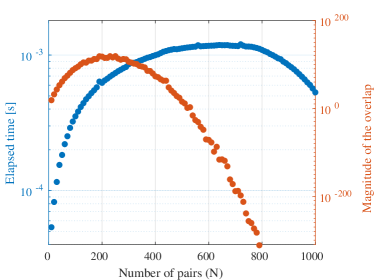
(b)

Figure 2: Mean of elapsed times (the left axes—blue), and magnitudes of the norm of AGP (the right axes—red) as a function of number of electron-pairs at some fixed number of levels. (a) $M=1000$ levels, $10\leq N\leq 1000$ pairs; (b) $M=100$ levels, $1\leq N\leq 100$ pairs. Every point is the mean of a random sample with $\eta_{p}\sim$ Unif(0,1) and $10^{3}$ observations.

The algorithm we use to calculate the ESP is one initially proposed by Fischer. Fischer (1974); Baker and Harwell (1996) This is the same summation algorithm used today in MATLAB’s poly function. Following the notation of Ref. Jiang et al. (2016) we call it sumESP. The sumESP algorithm takes advantage of the following property of ESP

$$S_{N}^{M}=S_{N}^{M-1}(\eta_{p}^{2})+\eta_{p}^{2}S_{N-1}^{M-1}(\eta_{p}^{2}).$$ (23)

Intuitively, Eq. (23) says that we can split any ESP into two sums such that one contains some arbitrary term $\eta_{p}^{2}$ in all of its summands and one that does not. In the context of quantum chemistry, Eq. (23) is mentioned in Ref. Staroverov and Scuseria (2002) However, there has been substantial progress in the computational and applied mathematics community to better understand and craft the algorithm. In particular, Ref. Rehman and Ipsen (2011) performed an error analysis and proved the stability of the algorithm. Ref. Jiang et al. (2016) made a slight improvement to the roundoff error bound and introduced new ways of calculating sumESP with enhanced precision. From these analyses it follows that sumESP is highly accurate and stable for positive summands Rehman and Ipsen (2011)—as is the case for the overlaps of AGP.

Quantitatively, one can say that, given $\{\eta_{1}^{2},...,\eta_{M}^{2}\}$ as a set of floating-point numbers, the “worst case" error due to sumESP is bounded above as follows Jiang et al. (2016)

$$\absolutevalue{\frac{S_{N}^{M}-S_{N}^{*M}}{S_{N}^{*M}}}\leq\frac{2(M-1)\epsilon}{1-2(M-1)\epsilon},$$ (24)

where $S_{N}^{*M}$ is the exact value of ESP and $S_{N}^{M}$ is computed using sumESP in floating-point arithmetic; $\epsilon$ denotes machine epsilon (unit roundoff). The error bound assumes that there are no numerical overflow and underflow occurring anywhere in the calculation. Rehman and Ipsen (2011) In practice, however, poor choice of normalization of $\eta_{p}$ could lead to overflow and/or underflow. For example, when $\eta_{p}^{2}>1$, the sum could overflow even for small values of $M$. Generally, sumESP is better conditioned when $\eta_{p}^{2}<1$; this is because the intermediate summations in the algorithm prevents the summands from getting too small. Nevertheless, because the sum is dominated by multiplications in $N>M/2$, one must watch for possible numerical underflow when $M$ is large and $N$ is close to $M$. And when $N<M/2$ the sum is dominated by additions, thus overflow is possible. Fortunately, issues of this kind can be resolved by scaling all geminal coefficients by some constant that prevents overflow or underflow without any hindrance to the method.

To make this analysis more quantitative, for $\eta_{p}\sim$ Unif(0,1), we have plotted the magnitude of sumESP (the same as the overlap of AGP) as a function of $M$ in Fig. 1. In Fig. 2 (the right axes), we fix $M=10^{2},10^{3}$ and vary $N$. It follows that in very large systems one must take caution when performing calculations away from $N\ll M$ or half-filling. But in moderate or small systems overflow and underflow should not be a concern. Indeed, the exact regimes in which overflow or underflow is expected highly depends on the distribution of geminal coefficients. Physically, the problem of overflow should be less likely because many of the geminal coefficients approach zero (e.g. near HF limit). And underflow is not of practical concern because in realistic calculations the number of orbitals should be greater than the number of electrons, i.e. $N\ll M$. With our experience using physical geminal coefficients in the pairing Hamiltonian, we have not yet observed overflow or underflow issues.

III.2 Runtime cost of an individual matrix element

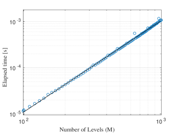
Figure 3: Asymptotic scaling of the norm of AGP at half-filling as a function of system size $M$. A linear fit to the log-log plot shows that the scaling is quadratic.

The cost of calculating a single matrix element of $n$-pair RDM is bounded above by the cost of the norm of AGP, i.e. $\langle AGP|AGP\rangle$. This is because all higher order RDMs require evaluation of lower degree ESPs by Eq. (20) and the cost of the prefactor is negligible. As such, to get the upper bound of the cost, we only report the elapsed time for evaluating the norm of AGP, which we refer to as the overlap. The theoretical cost of the overlap as a function of $N$ and $M$ grows as $N(1-N+M)-1$, which is the total number of iterations in the loops of the sumESP algorithm.

The left axes in Fig. 2 (the blue dots) illustrate the elapsed time of the overlap as a function of number of pairs, $N$. Every point in the plot is the sample mean of $10^{3}$ observation points with $\eta_{p}\sim$ Unif(0,1). By inspection, the most expensive computations occur when $N\approx M/2$ which is expected since ${M\choose N}$ is maximum when $N=M/2$. The shorter elapsed times in $N>M/2$ is due to fewer summations in the algorithm as $N$ approaches $M$.

To find the asymptotic scaling with system size, $M$, we fix $N=M/2$ and vary $M$ from $10^{2}$ to $10^{3}$. This gives the most expensive elapsed time for every value of $M$. The results are shown in Fig 3 in which every point is the sample mean of $10^{3}$ observations with $\eta_{p}\sim$ Unif(0,1). A linear fit to the log-log plot indicates that the asymptotic time scales quadratically, $T[s]\propto M^{1.97}$, with the system size, in line with the theoretical result.

III.3 Runtime cost of n-pair RDMs

(a)

(b)

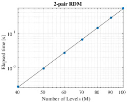
(c)

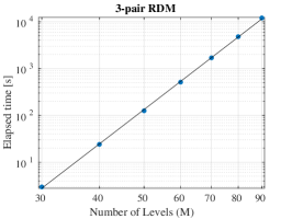
Figure 4: Time scales of computing $n=1,2,\text{and }3$ electron-pair RDMs in parallel using Algorithm 1 (see Appendix A). The black line is the linear fit to the log-log plot: (a) 1-pair RDM, $T[s]\propto M^{3.4}$; (b) 2-pair RDM, $T[s]\propto M^{5.7}$; (c) 3-pair RDM, $T[s]\propto M^{7.6}$.

Here, we report the maximum time needed for calculating all matrix elements of $n$-pair RDMs. At this juncture, we remind the reader that it is sufficient to merely compute and store ${\gamma}^{p_{1}<...<p_{n}}_{q_{1}<...<q_{n}}$. Since the calculations of the matrix elements are independent from each other, this is highly parallelizable. (See Appendix A for the pseudocode used to calculate the matrix elements.)

The theoretical cost of constructing an $n$-pair RDM on a single core is

$$\texttt{cost}\{\text{ $n$-pair RDM}\}\leq{M\choose n}^{2}\texttt{cost}\{\langle AGP|AGP\rangle\},$$ (25)

where ${M\choose n}^{2}$ is the number of matrix elements needed to construct an $n$-pair RDM with $M$ levels. Recall that the asymptotic cost of the norm of AGP is $\mathcal{O}(N(M-N))$.

In Fig. 4 we report the average elapsed time of $n$-pair RDM for $n=1,2,\text{and }3$, with $M\leq 100$. The plots show the sample average of 100 observations for $n=1,2$ and $10$ observations for $n=3$ in which $\eta_{p}\sim$ Unif(0,1).

IV Reconstruction formulae

In Sec. III.3 we argued that the asymptotic cost of constructing an $n$-pair RDM is $\mathcal{O}(NM^{2n+1})$. Here, we show a way of cutting down the cost by expressing higher order RDMs as a linear combination of lower order ones and geminal coefficients. This is an important ingredient for developing efficient correlated theories based on AGP, as most techniques require evaluation of high order RDMs. For example, in AGP based configuration interaction (AGP-CI) calculations done in our group Henderson and Scuseria (2019) up to to 5-body density matrices were needed (the Hamiltonian and the correlators contain 2-body operators each, and using the killers one can introduce a commutator to reduce the rank by 1). Therefore, a systematic way of reducing the scaling and the cost of calculating many-body RDMs is of great interest. Rosina mathematically anticipated Cioslowski (2000) that the 2-RDMs of AGP determine all of its higher order RDMs. As it turns out, we here show that 1-RDM occupation number RDMs ($\nu^{(1)}$) and $\eta$’s are sufficient to determine all RDMs of AGP.

Note that the decomposition method presented do not reflect vanishing cumulant decomposition of AGP density matrices. Also note that, the method differs from the decomposition of PBCS in which the density matrix is a weighted integral over the projection grid of a factorized transition density matrix. Scuseria et al. (2011)

IV.1 Direct decomposition

Our goal, here, is to express the nonzero elements of any $n$-pair RDM, ${\gamma}^{(n)}$, as a linear combination of ${{\nu}}^{(n^{\prime})}$ where $n\leq n^{\prime}\leq 2n$; then we show that we can further decompose each ${\nu}^{(n^{\prime})}$ into a sum of ${\nu}^{(1)}$, hence ${\gamma}^{(n)}\xrightarrow{}\sum{\nu}^{(1)}$.

Consider a nonzero element of an $n$-pair RDM, ${\gamma}^{p_{1}...p_{n}}_{q_{1}...q_{n}}$. In general, it can be that $p_{i}=q_{j}$ for some $i,j$. Since ${N}_{p}=2{P}^{\dagger}_{p}{P}_{p}$, we can write

$$\begin{split}{\gamma}^{p_{1}...p_{n}}_{q_{1}...q_{n}}={2^{-k}}\end{split}$$

$$\begin{split}\langle AGP|{P}^{\dagger}_{p_{1}}...{P}^{\dagger}_{p_{n-k}}{N}_{r_{1}}...{N}_{r_{k}}{P}_{q_{1}}...{P}_{q_{n-k}}|AGP\rangle,\end{split}$$ (26)

where $k$ is the number of common indices among $\{p_{i}\}$ and $\{q_{i}\}$. Written in this manner, we can assume all the remaining indices are different; otherwise the element is zero by construction. By this and hermiticity of ${\gamma}^{(n)}$, and the fact that the top and lower indices are permutable, we can further express

$$\begin{split}{\gamma}^{p_{1}...p_{n}}_{q_{1}...q_{n}}=\frac{1}{2^{n}}\langle AGP|{N}_{r_{1}}...{N}_{r_{k}}({P}^{\dagger}_{p_{1}}{P}_{q_{1}}+{P}^{\dagger}_{q_{1}}{P}_{p_{1}})\end{split}$$

$$\begin{split}...({P}^{\dagger}_{p_{n-k}}{P}_{q_{n-k}}+{P}^{\dagger}_{q_{n-k}}{P}_{p_{n-k}})|AGP\rangle.\end{split}$$ (27)

Now, by manipulating the killer of AGP, i.e. ${K}_{pq}|AGP\rangle=0$ reported in Ref. Henderson and Scuseria (2019) we can write

$$\begin{split}{P}^{\dagger}_{p}{P}_{q}+{P}^{\dagger}_{q}{P}_{p}=\end{split}$$

$$\begin{split}\frac{1}{\eta_{p}^{2}+\eta_{q}^{2}}\left({K}_{pq}^{\dagger}+{K}_{pq}+\eta_{p}\eta_{q}({N}_{p}+{N}_{q}-{N}_{p}{N}_{q})\right).\end{split}$$ (28)

By plugging Eq. (IV.1) into Eq. (IV.1) we arrive at an expression for ${\gamma}^{(n)}$ that is written purely as a linear combination of ${\nu}^{(n^{\prime})}$ and geminal coefficients as desired. Now, we decompose ${\nu}^{(n^{\prime})}$ into a sum of ${\nu}^{(1)}$ and factors of $\eta_{p}$. For this, we introduce a closed form expression which we prove in Appendix B

$${\nu}_{p_{1}...p_{n}}=\sum_{i=1}^{n}\left(\displaystyle\prod_{\begin{subarray}{c}j\geq 1\\ j\neq i\end{subarray}}^{n}\frac{2\eta_{p_{j}}^{2}}{\eta_{p_{j}}^{2}-\eta_{p_{i}}^{2}}\right){\nu}_{p_{i}}.$$ (29)

To make this discussion concrete, consider ${\gamma}^{(2)}$ as an example, whose non-zero elements can be written as

$${\gamma}^{pq}_{rs}=\begin{cases*}\langle{P}^{\dagger}_{p}{P}^{\dagger}_{q}{P}_{r}{P}_{s}\rangle&if $p,q\neq r,s$\\ \frac{1}{2}\langle{P}^{\dagger}_{p}{N}_{q}{P}_{r}\rangle&if $p\neq r$ and $q=s$\\ \frac{1}{4}\langle{N}_{p}{N}_{q}\rangle&if $p=r$ and $q=s$\\ \end{cases*}$$ (30)

For each of the three cases, we obtain an expression entirely in terms of the number RDMs and $\eta$’s using Eq. (IV.1):

$${\gamma}^{pq}_{rs}=\begin{cases*}\frac{\eta_{p}\eta_{q}\eta_{r}\eta_{s}}{4(\eta_{p}^{2}+\eta_{r}^{2})(\eta_{q}^{2}+\eta_{s}^{2})}\big{\langle}({N}_{p}+{N}_{r}-{N}_{p}{N}_{r})\\ ({N}_{q}+{N}_{s}-{N}_{q}{N}_{s})\big{\rangle}\\ \\ \frac{\eta_{p}\eta_{r}}{4(\eta_{p}^{2}+\eta_{r}^{2})}\big{(}\langle{N}_{p}{N}_{q}\rangle+\langle{N}_{q}{N}_{r}\rangle-\langle{N}_{p}{N}_{q}{N}_{r}\rangle\big{)}\\ \\ \frac{1}{4}\langle{N}_{p}{N}_{q}\rangle\end{cases*}$$ (31)

Then each of the $\langle{N}_{p}{N}_{q}\rangle$, $\langle{N}_{p}{N}_{q}{N}_{r}\rangle$, etc., can be inserted in Eq. (29) to produce an expression in terms of a linear combination of $\langle{{N}_{p}}\rangle$ and $\eta$’s only, as desired.

This result is profound as it implies that we can obtain all higher rank pair RDMs by merely computing ${\nu}^{(1)}$ whose cost grows asymptotically as $\mathcal{O}(M^{2}N)$ and may be computed only once for the rest of the calculations. The cost of prefactors is $n(n-1)$ which is negligible since for all practical purposes $n\ll N,M$. However, we pay the price of introducing $1/(\eta_{p}^{2}-\eta_{q}^{2})$ factors that can be numerically ill-posed when $\eta_{p}^{2}\approx\eta_{q}^{2}$ or when $\eta_{p},\eta_{q}\xrightarrow{}0$. In the regime that these factors are not problematic, the decomposition ${\gamma}^{(n)}\xrightarrow{}\sum{\nu}^{(1)}$ is a major improvement over computing all the matrix elements of an $n$-pair RDM. We must note that in our own implementation of these equations for practical problems (e.g. the attractive pairing Hamiltonian in Ref.Henderson and Scuseria (2019)) we have not observed these potential numerical issues.

IV.2 Stepwise decomposition

In practice, there are situations in which it is more advantageous to break down high rank RDMs in terms of “slightly" lower rank ones. This also makes the issue of having too many $1/(\eta_{p}^{2}-\eta_{q}^{2})$ factors less severe. To this end, we need a new notation for $\langle{P}^{\dagger}...{N}...{P}...\rangle$. Define

$$\begin{split}{Z}^{(k,m)}_{p_{1}...p_{t},\ r_{1}...r_{k},\ q_{1}...p_{t}}=\end{split}$$

$$\begin{split}\langle AGP|{P}^{\dagger}_{p_{1}}...{P}^{\dagger}_{p_{t}}{N}_{r_{1}}...{N}_{r_{k}}{P}_{q_{1}}...{P}_{q_{t}}|AGP\rangle,\end{split}$$ (32)

where $k$ is the number of ${N}_{p}$ operators in the middle, and $m$ is the total number of indices such that $k\leq m$. And define $t={(m-k)}/{2}$. For example,

$${Z}^{(0,6)}_{pqr,stu}=\langle AGP|{P}^{\dagger}_{p}{P}^{\dagger}_{q}{P}^{\dagger}_{r}{P}_{s}{P}_{t}{P}_{u}|AGP\rangle$$

$${Z}^{(1,5)}_{pq,r,st}=\langle AGP|{P}^{\dagger}_{p}{P}^{\dagger}_{q}{N}_{r}{P}_{s}{P}_{t}|AGP\rangle$$

$${Z}^{(2,4)}_{p,qr,s}=\langle AGP|{P}^{\dagger}_{p}{N}_{q}{N}_{r}{P}_{s}|AGP\rangle$$

$${Z}^{(3,3)}_{pqr}=\langle AGP|{N}_{p}{N}_{q}{N}_{r}|AGP\rangle.$$

Notice that the subscript indices on each $Z^{(k,m)}$ are all different; otherwise they are either zero or reducible to some other $Z^{(k^{\prime},m^{\prime})}$ by ${N}_{p}=2{P}^{\dagger}_{p}{P}_{p}$ and ${N}_{p}^{2}=2{N}_{p}$. Obviously all ${\gamma}^{(n)}$ can be mapped to $Z^{(k,2n-k)}$ for some $k$ and $n$, and vice versa.

Our goal, here, is to show that

$$Z^{(0,2n)} \xrightarrow{} \sum Z^{(1,2n-1)}\xrightarrow{}...\xrightarrow{}\;\sum Z^{(n,n)}=\sum{\nu}^{(n)}$$ (33)

$$\xrightarrow{} \sum{\nu}^{(n-1)}\xrightarrow{}....\xrightarrow{}\sum{\nu}^{(1)}.$$

As we prove in Appendix B, this can be accomplished by using the following formula at every step

$${Z}^{(k,m)}_{p_{1}...p_{t},\ r_{1}...r_{k},\ q_{1}...q_{t}}=\frac{\eta_{p_{i}}\eta_{q_{j}}}{2(\eta_{q_{j}}^{2}-\eta_{p_{i}}^{2})}\big{(}$$

$${Z}^{(k+1,m-1)}_{...p_{i-1}p_{i+1}...,\ r_{1}...r_{k}q_{j},\ ...q_{j-1}q_{j+1}...}-$$

$${Z}^{(k+1,m-1)}_{...p_{i-1}p_{i+1}...,\ p_{i}r_{1}...r_{k},\ ...q_{j-1}q_{j+1}...}\big{)},$$ (34)

where $i,j\in\{1,2,...t\}$. Similarly, it is easy to show that

$${\nu}_{p_{1}...p_{n}} = \frac{2\eta_{p_{j}}^{2}}{\eta_{p_{j}}^{2}-\eta_{p_{i}}^{2}}{\nu}_{p_{1}...p_{j-1}p_{j+1}...p_{n}}$$ (35)

$$+ \frac{2\eta_{p_{i}}^{2}}{\eta_{p_{i}}^{2}-\eta_{p_{j}}^{2}}{\nu}_{p_{1}...p_{i-1}p_{i+1}...p_{n}},$$

here, $i,j\in\{1,2,...n\}$.

The advantage of breaking down the density matrices like this is that, at every step, we reduce the dimension by one, thereby reducing the asymptotic scaling of computing it by a factor of $M^{2}$ and a negligible prefactor. Moreover, we can stop at any step of our choice based on the cost that we are willing to tolerate.

V Runtime of Energy and AGP-CI

Figure 5: Runtime measurement of the pairing Hamiltonian energy with and without the reconstruction formula. Each point is the sample mean of 100 observations with $\eta_{p}\sim\text{Unif}(0,1)$.

In this section, we benchmark the speed gain when using the reconstruction formulae. Here, we report the runtime measurements of two calculations: (1) the energy of the pairing Hamiltonian (reduced BCS); (2) AGP-CI calculations as reported in Ref. Henderson and Scuseria (2019). See Appendix C for the computer environments used in these benchmarks.

We start with the pairing Hamiltonian. Recall that the attractive pairing Hamiltonian can be written as follows: Degroote et al. (2016)

$${H}=\sum_{p}\epsilon_{p}{N}_{p}-G\sum_{pq}{P}^{\dagger}_{p}{P}_{q}.$$ (36)

The expected value of the energy over AGP in terms of the pair RDMs is

$$E=\sum_{p}{\gamma}^{p}_{p}(2\epsilon_{p}-G)-2G\sum_{p<q}{\gamma}^{p}_{q}.$$ (37)

And using the reconstruction formulae, we can get

$$E=\sum_{p}{\nu}_{p}(\epsilon_{p}-\frac{G}{2})-G\sum_{p<q}\frac{\eta_{p}\eta_{q}}{\eta_{p}^{2}-\eta_{q}^{2}}({\nu}_{p}-{\nu}_{q}).$$ (38)

Fig. 5 shows the elapsed time differences between implementing Eq. (37) and Eq. (38) as a function of number of levels at half-filling. For each case, the corresponding RDM is stored and then called in the calculation. By inspection, it is easy to see that the reconstruction formulae speed up the calculations often by an order of magnitude. Obviously, the improvement becomes more noticeable as the number of levels increases.

At last, we report the elapsed time of performing AGP-CI calculations with and without the reconstruction formulae in Fig. 6. For these calculations, we stored up to $4$-indexed RDMs in memory and calculated all the rank 5 RDMs using the direct decomposition formula Eq. (29). Here, $\eta$’s are optimized beforehand for the pairing Hamiltonian ($G=2$) for various values of $M$. Similar to the energy calculations, we observe that the reconstruction formulae lead to a substantial improvement.

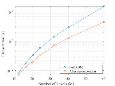
Figure 6: Runtime cost of AGP-CI calculation with and without the reconstruction formula. Every point is the mean of the same calculation repeated $200$ times.

VI Conclusions

Analytic expressions of the norm and reduced density matrices of AGP wavefunction are proportional to ESP. We used the sumESP algorithm Rehman and Ipsen (2011); Jiang et al. (2016) to efficiently calculate ESPs and argued that, with appropriate normalization, it is well suited for physical problems wherein $N\ll M$. We have shown that our method can reliably calculate the norm and elements of RDMs to all ranks for systems as large as a few thousand orbitals and hundreds of electrons. Our runtime measurements indicate that the asymptotic cost per element of an $n$-pair RDMs is at most quadratic, and the cost of building an $n$-pair RDM grows asymptotically as $\mathcal{O}(NM^{2n+1})$.

However, to reduce the cost of computing the RDMs even further, we have derived reconstruction formulae that allow decomposition of any RDM into a linear combinations of lower rank ones and geminal coefficients. We introduced two methods: (1) Direct decomposition—breaks down a high rank pair RDM in terms of linear combination of rank-1 occupation RDMs; (2) Stepwise decomposition—reduces the dimension of a RDM by one at every step thereby reducing the cost of computing it by a factor of $M^{2}$.

We demonstrate the advantage of using our reconstruction formulae by benchmarking it against the energy of the pairing Hamiltonian and AGP-CI calculation without the reconstruction formulae. The numerical results indicate that, indeed, the reconstruction formulae lead to a substantial speed-up, especially in systems with large number of orbitals.

Appendix A Numerical Implementation

Below is a pseudocode for calculating a single matrix element of an $n$-pair RDM. Implementation of sumESP is taken from Ref. Jiang et al. (2016)

input : $\mathbf{x}=\{\eta_{1},..,\eta_{M}\}$;

$N$: number of pairs;

$L=\{p_{1},...p_{n},q_{1},...,q_{n}\}$

output :  ${\gamma}^{p_{1}...p_{n}}_{q_{1},...q_{n}}$

 

integer $i,j,k,n,N,M$;  real $p$

integer array $(L_{i})_{1:2n}$

real array $(L_{i})_{1:2n}$, $(x_{i})_{1:M}$, $(S_{j}^{i})_{(i\in 1:M)(j\in 1:N+1)}$

if  $(p_{i}=p_{j}$ or $q_{i}=q_{j})$ or $(n>N)$  then

       Output = 0;

      End the program;

end if

$k\xleftarrow{}N-size(L)/2$; // $size(x)$ gives the size of $x$

$p\xleftarrow{}(\prod_{i\in L}x_{i}$);

$x\xleftarrow{}eliminate(x_{i\in L})$ // removes $x_{i\in L}$ from $x$

$x\xleftarrow{}x^{2}$

// Below is the sumESP algorithm

$M\xleftarrow{}size(x)$;

$S_{j}^{i}\xleftarrow{}$ zeros for $j>i$; $S_{0}^{i}\xleftarrow{}1$ for $1\leq i\leq M-1$;

$S_{1}^{1}\xleftarrow{}x_{1};$

for i = 2 to M do

       for

References

- Surján (1999) P. R. Surján, in Correlation and Localization, Topics in Current Chemistry, edited by P. R. Surján, R. J. Bartlett, F. Bogár, D. L. Cooper, B. Kirtman, W. Klopper, W. Kutzelnigg, N. H. March, P. G. Mezey, H. Müller, J. Noga, J. Paldus, J. Pipek, M. Raimondi, I. Røeggen, J. Q. Sun, P. R. Surján, C. Valdemoro, and S. Vogtner (Springer Berlin Heidelberg, Berlin, Heidelberg, 1999) pp. 63–88.
- Coleman (1965) A. J. Coleman, Journal of Mathematical Physics 6, 1425 (1965).
- Ring and Schuck (1980) P. Ring and P. Schuck, The Nuclear Many-Body Problem, Theoretical and Mathematical Physics, The Nuclear Many-Body Problem (Springer-Verlag, Berlin Heidelberg, 1980).
- Blaizot and Ripka (1986) J.-P. Blaizot and G. Ripka, Quantum theory of finite systems (MIT Press, Cambridge, Mass., 1986) oCLC: 11865956.
- Yang (1962) C. N. Yang, Rev. Mod. Phys. 34, 694 (1962).
- Bardeen et al. (1957) J. Bardeen, L. N. Cooper, and J. R. Schrieffer, Phys. Rev. 108, 1175 (1957).
- Veillard and Clementi (1967) A. Veillard and E. Clementi, Theoret. Chim. Acta 7, 133 (1967).
- Couty and Hall (1997) M. Couty and M. B. Hall, J. Phys. Chem. A 101, 6936 (1997).
- Kollmar and Heß (2003) C. Kollmar and B. A. Heß, J. Chem. Phys. 119, 4655 (2003).
- Bytautas et al. (2011) L. Bytautas, T. M. Henderson, C. A. Jiménez-Hoyos, J. K. Ellis, and G. E. Scuseria, J. Chem. Phys. 135, 044119 (2011).
- Sheikh and Ring (2000) J. A. Sheikh and P. Ring, Nuclear Physics A 665, 71 (2000).
- Scuseria et al. (2011) G. E. Scuseria, C. A. Jiménez-Hoyos, T. M. Henderson, K. Samanta, and J. K. Ellis, J. Chem. Phys. 135, 124108 (2011).
- Richardson (1963) R. W. Richardson, Physics Letters 3, 277 (1963).
- Dukelsky et al. (2004) J. Dukelsky, S. Pittel, and G. Sierra, Rev. Mod. Phys. 76, 643 (2004).
- Johnson et al. (2013) P. A. Johnson, P. W. Ayers, P. A. Limacher, S. D. Baerdemacker, D. V. Neck, and P. Bultinck, Computational and Theoretical Chemistry Reduced Density Matrices: A Simpler Approach to Many-Electron Problems?, 1003, 101 (2013).
- Limacher et al. (2013) P. A. Limacher, P. W. Ayers, P. A. Johnson, S. De Baerdemacker, D. Van Neck, and P. Bultinck, J. Chem. Theory Comput. 9, 1394 (2013).
- Henderson et al. (2014) T. M. Henderson, G. E. Scuseria, J. Dukelsky, A. Signoracci, and T. Duguet, Phys. Rev. C 89, 054305 (2014).
- Henderson et al. (2015) T. M. Henderson, I. W. Bulik, and G. E. Scuseria, J. Chem. Phys. 142, 214116 (2015).
- Degroote et al. (2016) M. Degroote, T. M. Henderson, J. Zhao, J. Dukelsky, and G. E. Scuseria, Phys. Rev. B 93, 125124 (2016).
- Qiu et al. (2019) Y. Qiu, T. M. Henderson, T. Duguet, and G. E. Scuseria, Phys. Rev. C 99, 044301 (2019).
- Henderson and Scuseria (2019) T. M. Henderson and G. E. Scuseria, J. Chem. Phys. 151, 051101 (2019).
- Fischer (1974) G. H. Fischer, Einführung in die Theorie psychologischer Tests [Introduction to the theory of psychological tests] (Bern Huber, 1974).
- Rehman and Ipsen (2011) R. Rehman and I. Ipsen, SIAM J. Matrix Anal. Appl. 32, 90 (2011).
- Jiang et al. (2016) H. Jiang, S. Graillat, R. Barrio, and C. Yang, Applied Mathematics and Computation 273, 1160 (2016).
- Dietrich et al. (1964) K. Dietrich, H. J. Mang, and J. H. Pradal, Phys. Rev. 135, B22 (1964).
- Ma and Rasmussen (1977) C. W. Ma and J. O. Rasmussen, Phys. Rev. C 16, 1179 (1977).
- Weiner and Goscinski (1980) B. Weiner and O. Goscinski, Phys. Rev. A 22, 2374 (1980).
- Ortiz et al. (1981) J. V. Ortiz, B. Weiner, and Y. Öhrn, International Journal of Quantum Chemistry 20, 113 (1981).
- Cioslowski (2000) J. Cioslowski, ed., Many-Electron Densities and Reduced Density Matrices, Mathematical and Computational Chemistry (Springer US, 2000).
- Gilmore (2008) R. Gilmore, Lie Groups, Physics, and Geometry: An Introduction for Physicists, Engineers and Chemists (Cambridge University Press, 2008).
- Lee (2016) H. Lee, Linear Algebra and its Applications 492, 89 (2016).
- Baker and Harwell (1996) F. B. Baker and M. R. Harwell, Applied Psychological Measurement 20, 169 (1996).
- Staroverov and Scuseria (2002) V. N. Staroverov and G. E. Scuseria, J. Chem. Phys. 117, 11107 (2002).