ISL: A novel approach for deep exploration

Lucas C. Cassano
Department of Electrical and Computer Engineering
University of California
Los Angeles, USA
cassanolucas@ucla.edu
&Ali H. Sayed
School of Engineering
École Polytechnique Fédérale de Lausanne
CH-1015 Lausanne, Switzerland
ali.sayed@epfl.ch
The author is also with EPFL.
Abstract

In this article we explore an alternative approach to address deep exploration and we introduce the ISL algorithm, which is efficient at performing deep exploration. Similarly to maximum entropy RL, we derive the algorithm by augmenting the traditional RL objective with a novel regularization term. A distinctive feature of our approach is that, as opposed to other works that tackle the problem of deep exploration, in our derivation both the learning equations and the exploration-exploitation strategy are derived in tandem as the solution to a well-posed optimization problem whose minimization leads to the optimal value function. Empirically we show that our method exhibits state of the art performance on a range of challenging deep-exploration benchmarks.

1 Introduction

Reinforcement learning is concerned with designing algorithms that seek to maximize long term cumulative rewards by interacting with an environment of unknown dynamics. Recently, significant progress has been made in deep RL (the combination of RL algorithms with Deep Learning). In particular, several algorithms have been introduced based on the maximum entropy framework [1, 2, 3, 4, 5, 6, 7]. In maximum entropy RL, the traditional RL objective is augmented with the entropy of the learned policy, which is weighted by a temperature parameter. The main benefit of the maximum RL framework is that it allows to derive algorithms that are more sample efficient (because they operate off-policy) than policy gradients algorithms like A3C [8], TRPO [9] and PPO [10] and exhibit improved stability over algorithms based on Q-learning. Furthermore, it has been demonstrated empirically that algorithms based on the maximum entropy framework have improved exploration capabilities [2].

Although these recent algorithms have shown state of the art performance in several tasks, they are not without shortcomings. In the first place, augmenting the original RL objective with the entropy bonuses biases the solution of the optimization problem. This could be solved by slowly annealing the temperature parameter, but it is unclear what is the best way to do so and how this change affects convergence speed. The second, and more important, shortcoming is that although these algorithms have improved exploration capabilities, they are still unable to perform deep exploration (i.e., they tend to perform poorly in environments with very sparse reward structures). These difficulties suggest that there may not be sufficient theoretical justification for the use of the policy’s entropy as the regularizer for the RL objective, which in turn raises the question of whether another regularizer could help address the two aforementioned challenges. In this work we explore this possibility and connect the problem of deep exploration with that of maximum entropy RL. Traditionally, the problem of deriving deep exploration strategies has been treated separately from that of deriving the learning equations [11, 12, 13, 14, 15]. In this article we show that both the learning equations and the exploration strategy can be derived in tandem as the solution to a well-posed optimization problem whose minimization leads to the optimal value function. We do this by augmenting the objective function with a novel regularizer. Instead of using the policy’s entropy as the regularizer (as maximum entropy RL does), we use a function which depends on the uncertainties over the agent’s estimates of the q𝑞q values.

The contribution of this paper is the introduction of an alternative approach to address deep exploration and the introduction of an algorithm that we refer to as the Information Seeking Learner (ISL). This algorithm has a similar form to soft RL algorithms like SAC and SBEED, but the fundamental difference is that it explicitly estimates the uncertainties of its q𝑞q estimates and uses these uncertainties to drive deep exploration.

1.1 Relation to prior work

ISL is related to recent work on maximum entropy algorithms [1, 2, 3, 4, 5, 6]. All these algorithms augment the traditional RL objective with a term that aims to maximize the entropy of the learned policy, which is weighted by a temperature parameter. The consequence of using this augmented objective is two-fold. First, it allows to derive off-policy algorithms with improved stability compared to algorithms based on Q-learning. Second, it improves the exploration properties of the algorithms. However, using this augmented objective has two main drawbacks. First, the policy to which these algorithms converge is biased away from the true optimal policy. This point can be handled by annealing the temperature parameter but this can slow down convergence and compromise exploration. Furthermore, it is unclear what the optimal schedule to perform annealing is and how it affects the conditioning of the optimization problem. Secondly, although exploration is improved, algorithms derived from this modified cost are not efficient at performing deep exploration. The reason for this is that a unique temperature parameter is used for all states. In order to perform deep exploration it is necessary to have a scheme that allows agents to learn policies that exploit more in states where the agent has high confidence in the optimal action (in order to be able to reach further novel states with high probability) and act in a more exploratory manner in unknown states. In [16] the authors explore this possibility in a tabular setting making the temperature parameter state dependent and annealing it progressively as states are explored; however, the annealing schedule is determined heuristically and it is unclear what would be an effective way to do so when using function approximation. The relation between ISL and these works is that we also augment the RL objective with an entropy based regularizer and as a consequence we derive a an algorithm that relies on a soft backup. Under our scheme, agents converge to the true optimal policy without the need for annealing any parameter and, moreover, an exploration strategy is derived that is capable of performing deep exploration.

Our paper is also related to works on deep exploration strategies. One line of research is based on posterior sampling for RL [12, 13, 15]. The main idea in these works is to sample the value function from a posterior distribution over such function. The common point between these works and ours is that deep exploration is driven by some measure of the uncertainty on the estimated value function. One difference between these works and ours is that they rely on Posterior Sampling while our work does not. Another fundamental difference is that these works treat the exploration problem separately from the derivation of the learning rules. In other words, they use heuristics based on randomised value functions to drive exploration but use off-the-shelf learning rules like Q-learning. In our approach, we use the uncertainty over the learned value function not only to drive exploration but to formulate a new objective from which we derive a new learning rule. Another line of work relies on pseudo-counts [17, 18], the fundamental limitation of this approach is that it only performs good if the generalization of the density model is aligned with the task objective [15]. Another line of research relies on IRs [11, 19, 20, 21], these rewards are based on some heuristic based proxy that reflects the novelty of a state. ISL can also be seen as utilizing IRs, however there are two main differences with the previous works. Firstly, we use IRs that depend on the uncertainty of the q𝑞q function. Secondly, we never actually compute IRs, but rather we rely on a different backup to update the q𝑞q estimates (this point is clarified in section 3).

2 Preliminaries

We consider the problem of policy optimization within the traditional RL framework. We model our setting as a Markov Decision Process (MDP), with an MDP defined by (𝒮𝒮\mathcal{S},𝒜𝒜\mathcal{A},𝒫𝒫\mathcal{P},r𝑟r), where 𝒮𝒮\mathcal{S} is a set of states, 𝒜𝒜\mathcal{A} is a set of actions of size A=|𝒜|𝐴𝒜A=|\mathcal{A}|, 𝒫(s|s,a)𝒫conditionalsuperscript𝑠𝑠𝑎\mathcal{P}(s^{\prime}|s,a) specifies the probability of transitioning to state s𝒮superscript𝑠𝒮s^{\prime}\in\mathcal{S} from state s𝒮𝑠𝒮s\in\mathcal{S} having taken action a𝒜𝑎𝒜a\in\mathcal{A}, and r:𝒮×𝒜×𝒮:𝑟𝒮𝒜𝒮r:\mathcal{S}\times\mathcal{A}\times\mathcal{S}\rightarrow\mathbb{R} is the reward mapping r(s,a,s)𝑟𝑠𝑎superscript𝑠r(s,a,s^{\prime}).

Assumption 1.

rminr(s,a,s)rmax,subscript𝑟𝑟𝑠𝑎superscript𝑠subscript𝑟r_{\min}\leq r(s,a,s^{\prime})\leq r_{\max}, (s,a,s)for-all𝑠𝑎superscript𝑠\forall(s,a,s^{\prime}).

In this work we consider the maximization of the discounted infinite reward as the objective of the RL agent:

π(a|s)=argmaxπ𝔼𝒫,π(t=0γt𝒓(𝒔t,𝒂t,𝒔t+1)|𝒔0=s)superscript𝜋conditional𝑎𝑠subscriptargmax𝜋subscript𝔼𝒫𝜋conditionalsuperscriptsubscript𝑡0superscript𝛾𝑡𝒓subscript𝒔𝑡subscript𝒂𝑡subscript𝒔𝑡1subscript𝒔0𝑠\pi^{\dagger}(a|s)=\operatorname*{arg\,max}_{\pi}\mathbb{E}\hskip 1.42271pt_{\mathcal{P},\pi}\bigg{(}\sum_{t=0}^{\infty}\gamma^{t}\mbox{\boldmath$r$}(\mbox{\boldmath$s$}_{t},\mbox{\boldmath$a$}_{t},\mbox{\boldmath$s$}_{t+1})\big{|}\mbox{\boldmath$s$}_{0}=s\bigg{)} (1)

where π(a|s)superscript𝜋conditional𝑎𝑠\pi^{\dagger}(a|s) is the optimal policy, γ[0,1)𝛾01\gamma\in[0,1) is the discount factor and 𝒔tsubscript𝒔𝑡\mbox{\boldmath$s$}_{t} and 𝒂tsubscript𝒂𝑡\mbox{\boldmath$a$}_{t} are the state and action at time t𝑡t, respectively. We clarify that in this work, random variables are always denoted in bold font. We recall that each policy π𝜋\pi has an associated state value function vπ(s)superscript𝑣𝜋𝑠v^{\pi}(s) and state-action value function qπ(s,a)superscript𝑞𝜋𝑠𝑎q^{\pi}(s,a),111In this paper we will refer to both vπ(s)superscript𝑣𝜋𝑠v^{\pi}(s) and qπ(s,a)superscript𝑞𝜋𝑠𝑎q^{\pi}(s,a) as value functions indistinctly. and that value functions corresponding to the optimal policy are given by [22]:

q(s,a)=r(s,a)+γ𝔼𝒫maxaq(𝒔,a),π(a|s)=argmaxπaπ(a|s)q(s,a)formulae-sequencesuperscript𝑞𝑠𝑎𝑟𝑠𝑎𝛾subscript𝔼𝒫subscriptsuperscript𝑎superscript𝑞superscript𝒔superscript𝑎superscript𝜋conditional𝑎𝑠subscriptargmax𝜋subscript𝑎𝜋conditional𝑎𝑠superscript𝑞𝑠𝑎\displaystyle q^{\dagger}(s,a)=r(s,a)+\gamma\mathbb{E}\hskip 1.42271pt_{\mathcal{P}}\max_{a^{\prime}}q^{\dagger}(\mbox{\boldmath$s$}^{\prime},a^{\prime}),\hskip 14.22636pt\pi^{\dagger}(a|s)=\operatorname*{arg\,max}_{\pi}\sum_{a}\pi(a|s)q^{\dagger}(s,a) (2)

where for convenience we defined r(s,a)=𝔼𝒓(s,a,𝒔)𝑟𝑠𝑎𝔼𝒓𝑠𝑎superscript𝒔r(s,a)=\mathbb{E}\hskip 1.42271pt\mbox{\boldmath$r$}(s,a,\mbox{\boldmath$s$}^{\prime}).

3 Algorithm derivation

Equations (2) are useful to derive algorithms for planning problems (i.e., problems in which the reward function and transition kernel are known) but may be unfit to derive RL algorithms because they mask the fact that the agent relies on estimated quantities (which are subject to uncertainty). Hence, in this work, we modify (1) to reflect the fact that an RL agent is constrained by the uncertainty of its estimates. Intuitively, we change the goal of the agent to not just maximize the discounted cumulative rewards but also to collect information about the MDP in order to minimize the uncertainty of its estimated quantities. For this purpose, we assume that at any point in time the agent has some estimate of the optimal value function denoted by q^(s,a)^𝑞𝑠𝑎\widehat{q}(s,a), which is subject to some error q~(s,a)=q(s,a)q^(s,a)~𝑞𝑠𝑎superscript𝑞𝑠𝑎^𝑞𝑠𝑎\widetilde{q}(s,a)=q^{\dagger}(s,a)-\widehat{q}(s,a). We model the unknown quantities q~(s,a)~𝑞𝑠𝑎\widetilde{q}(s,a) as random variables. More specifically, for each state-action pair we assume 𝒒~(s,a)bold-~𝒒𝑠𝑎\boldsymbol{\widetilde{q}}(s,a) follows a uniform probability distribution with zero mean 𝒒~(s,a)U(0,(s,a))similar-tobold-~𝒒𝑠𝑎U0𝑠𝑎\boldsymbol{\widetilde{q}}(s,a)\sim\textrm{U}(0,\ell(s,a)) such that:

q~(s,a)[q^(s,a)(s,a);q^(s,a)+(s,a)]~𝑞𝑠𝑎^𝑞𝑠𝑎𝑠𝑎^𝑞𝑠𝑎𝑠𝑎\displaystyle\widetilde{q}(s,a)\in[\widehat{q}(s,a)-\ell(s,a);\widehat{q}(s,a)+\ell(s,a)] (3)

We will refer to the probability density function of 𝒒~(s,a)bold-~𝒒𝑠𝑎\boldsymbol{\widetilde{q}}(s,a) as d(s,a)(q~)subscript𝑑𝑠𝑎~𝑞d_{(s,a)}(\widetilde{q}). We assume zero mean uniform distributions for the following reasons. First, if the mean were different than zero, it could be used to improve the estimate q^(s,a)^𝑞𝑠𝑎\widehat{q}(s,a) as q^(s,a)q^(s,a)+𝔼𝒒~(s,a)^𝑞𝑠𝑎^𝑞𝑠𝑎𝔼bold-~𝒒𝑠𝑎\widehat{q}(s,a)\leftarrow\widehat{q}(s,a)+\mathbb{E}\hskip 1.42271pt\boldsymbol{\widetilde{q}}(s,a) resulting in a new estimate whose corresponding error would be zero mean. Secondly, under assumption 1, we know that for any infinitely discounted MDP, a symmetric bound for the error of the value function exists in the form (s,a)<𝒒~(s,a)<(s,a)𝑠𝑎bold-~𝒒𝑠𝑎𝑠𝑎-\ell(s,a)<\boldsymbol{\widetilde{q}}(s,a)<\ell(s,a).222This is due to the fact that the value functions are lower and upper bounded by rmin/(1γ)subscript𝑟min1𝛾r_{\textrm{min}}/(1-\gamma) and rmax/(1γ)subscript𝑟1𝛾r_{\max}/(1-\gamma). Moreover, typically there is no prior information about the error distribution between these bounds and therefore a non-informative uniform distribution becomes appropriate.

We further define the state uncertainty distribution usπ(q~)superscriptsubscript𝑢𝑠𝜋~𝑞u_{s}^{\pi}(\widetilde{q}) (which is given by a mixture of the state-action error distributions) and the Maximum-Uncertainty-Entropy policy πsuperscript𝜋\pi^{\bullet} (which at every state chooses the action whose corresponding 𝒒~(s,a)bold-~𝒒𝑠𝑎\boldsymbol{\widetilde{q}}(s,a) has the greatest uncertainty):

usπ(q~)=𝔼πd(s,𝒂)(q~),π(a|s)={1, if (s,a)=maxa(s,a)0, elseformulae-sequencesuperscriptsubscript𝑢𝑠𝜋~𝑞subscript𝔼𝜋subscript𝑑𝑠𝒂~𝑞superscript𝜋conditional𝑎𝑠cases1 if 𝑠𝑎subscript𝑎𝑠𝑎otherwise0 elseotherwise\displaystyle u_{s}^{\pi}(\widetilde{q})=\mathbb{E}\hskip 1.42271pt_{\pi}d_{(s,\boldsymbol{a})}(\widetilde{q}),\hskip 28.45274pt\pi^{\bullet}(a|s)=\begin{cases}1,\text{ if }\hskip 5.69054pt\ell(s,a)=\max_{a}\ell(s,a)\\ 0,\text{ else}\end{cases} (4)

We thus define the goal of our reinforcement learning agent to be:

π(a|s)superscript𝜋conditional𝑎𝑠\displaystyle\pi^{\star}(a|s) =argmaxπ𝔼𝒫,π(t=0γt[𝒓(𝒔t,𝒂t,𝒔t+1)κDKL(u𝒔tπ(q~)||u𝒔t(q~))]|𝒔0=s)\displaystyle=\operatorname*{arg\,max}_{\pi}\mathbb{E}\hskip 1.42271pt_{\mathcal{P},\pi}\bigg{(}\sum_{t=0}^{\infty}\gamma^{t}\big{[}\mbox{\boldmath$r$}(\mbox{\boldmath$s$}_{t},\mbox{\boldmath$a$}_{t},\mbox{\boldmath$s$}_{t+1})-\kappa D_{KL}(u_{\mbox{\boldmath$s$}_{t}}^{\pi}(\widetilde{q})||u_{\mbox{\boldmath$s$}_{t}}^{\bullet}(\widetilde{q}))\big{]}\Big{|}\mbox{\boldmath$s$}_{0}=s\bigg{)} (5)

where κ𝜅\kappa is a positive regularization parameter, DKLsubscript𝐷𝐾𝐿D_{KL} is the Kullback-Leibler divergence, and u𝒔t(q~)superscriptsubscript𝑢subscript𝒔𝑡~𝑞u_{\mbox{\boldmath$s$}_{t}}^{\bullet}(\widetilde{q}) is the state uncertainty distribution corresponding to πsuperscript𝜋\pi^{\bullet}. In this work we refer to π(a|s)superscript𝜋conditional𝑎𝑠\pi^{\star}(a|s) as the uncertainty constrained optimal policy (or uc-optimal policy). Under this new objective, we redefine the value functions as:

qπ(s,a)=r(s,a)+γ𝔼𝒫vπ(𝒔)superscript𝑞𝜋𝑠𝑎𝑟𝑠𝑎𝛾subscript𝔼𝒫superscript𝑣𝜋superscript𝒔\displaystyle q^{\pi}(s,a)=r(s,a)+\gamma\mathbb{E}\hskip 1.42271pt_{\mathcal{P}}v^{\pi}(\mbox{\boldmath$s$}^{\prime}) (6a)
vπ(s)=𝔼(t=0γt[𝒓(𝒔t,𝒂t,𝒔t+1)κDKL(u𝒔tπ(q~))]|𝒔0=s)=𝔼(r(s,a)κDKL(usπ(q~))+γvπ(𝒔))superscript𝑣𝜋𝑠𝔼conditionalsuperscriptsubscript𝑡0superscript𝛾𝑡delimited-[]𝒓subscript𝒔𝑡subscript𝒂𝑡subscript𝒔𝑡1𝜅subscript𝐷𝐾𝐿superscriptsubscript𝑢subscript𝒔𝑡𝜋~𝑞subscript𝒔0𝑠𝔼𝑟𝑠𝑎𝜅subscript𝐷𝐾𝐿superscriptsubscript𝑢𝑠𝜋~𝑞𝛾superscript𝑣𝜋superscript𝒔bold-′\displaystyle v^{\pi}(s)=\mathbb{E}\hskip 1.42271pt\bigg{(}\sum_{t=0}^{\infty}\gamma^{t}\big{[}\mbox{\boldmath$r$}(\mbox{\boldmath$s$}_{t},\mbox{\boldmath$a$}_{t},\mbox{\boldmath$s$}_{t+1})-\kappa D_{KL}(u_{\mbox{\boldmath$s$}_{t}}^{\pi}(\widetilde{q}))\big{]}\big{|}\mbox{\boldmath$s$}_{0}=s\bigg{)}=\mathbb{E}\hskip 1.42271pt\big{(}r(s,a)-\kappa D_{KL}(u_{s}^{\pi}(\widetilde{q}))+\gamma v^{\pi}(\boldsymbol{s^{\prime}})\big{)} (6b)

where, with a little abuse of notation, we defined DKL(usπ(q~))=ΔDKL(usπ(q~)||us(q~))D_{KL}(u_{s}^{\pi}(\widetilde{q}))\stackrel{{\scriptstyle\Delta}}{{=}}D_{KL}(u_{s}^{\pi}(\widetilde{q})||u_{s}^{\bullet}(\widetilde{q})). Using (6) we can rewrite (5) as:

πsuperscript𝜋\displaystyle\pi^{\star} =argmaxπaπ(a|s)q^(s,a)κDKL(usπ(q~))absentsubscriptargmax𝜋subscript𝑎𝜋conditional𝑎𝑠^𝑞𝑠𝑎𝜅subscript𝐷𝐾𝐿superscriptsubscript𝑢𝑠𝜋~𝑞\displaystyle=\operatorname*{arg\,max}_{\pi}\sum_{a}\pi(a|s)\widehat{q}(s,a)-\kappa D_{KL}(u_{s}^{\pi}(\widetilde{q})) (7)

Note that the exploration-exploitation trade-off becomes explicit in (7). To maximize the first term of the summation in (7), the agent has to exploit its knowledge of q^^𝑞\widehat{q}, while to maximize the second term, the agent’s policy needs to match πsuperscript𝜋\pi^{\bullet}, which is a policy that seeks to maximize the information gathered through exploration. Since the argument being maximized in (7) is differentiable with respect to π(a|s)𝜋conditional𝑎𝑠\pi(a|s) we can obtain a closed-form expression for πsuperscript𝜋\pi^{\star}. Before presenting such closed-form expression we introduce the following useful remark, lemmas and definitions.

Remark 1.

In the interest of simplifying equations and notation we clarify that from now on we will use i(s)=Δ(s,ai)superscriptΔsubscript𝑖𝑠𝑠subscript𝑎𝑖\ell_{i}(s)\stackrel{{\scriptstyle\Delta}}{{=}}\ell(s,a_{i}) and even i=Δ(s,ai)superscriptΔsubscript𝑖𝑠subscript𝑎𝑖\ell_{i}\stackrel{{\scriptstyle\Delta}}{{=}}\ell(s,a_{i}) when the state s𝑠s is clear from the context.

Lemma 1.

Assuming the actions are ordered such that i>ji>jiffsubscript𝑖subscript𝑗𝑖𝑗\ell_{i}>\ell_{j}\iff i>j, the KL divergence term in (7) for a given state s𝑠s is given by:

n=1A(nn1)(k=nAπ(ak|s)k)log[b=nAπ(b|s)Ab]superscriptsubscript𝑛1𝐴subscript𝑛subscript𝑛1superscriptsubscript𝑘𝑛𝐴𝜋conditionalsubscript𝑎𝑘𝑠subscript𝑘superscriptsubscript𝑏𝑛𝐴𝜋conditional𝑏𝑠subscript𝐴subscript𝑏\displaystyle\sum_{n=1}^{A}(\ell_{n}-\ell_{n-1})\left(\sum_{k=n}^{A}\frac{\pi(a_{k}|s)}{\ell_{k}}\right)\log\left[\sum_{b=n}^{A}\frac{\pi(b|s)\ell_{A}}{\ell_{b}}\right] (8)
Proof.

The proof is included in Appendix 6.1. 

Definition 1.

Pareto dominated action: For a certain state sss we say that an action ajsubscriptaja_{j} is Pareto dominated by action aisubscriptaia_{i} if q^(s,aj)q^(s,ai)^qssubscriptaj^qssubscriptai\widehat{q}(s,a_{j})\leq\widehat{q}(s,a_{i}) and (s,aj)<(s,ai)ssubscriptajssubscriptai\ell(s,a_{j})<\ell(s,a_{i}).

Definition 2.

Mixed Pareto dominated action: For a certain state sss we say that an action aksubscriptaka_{k} is mixed Pareto dominated if there exist two actions aisubscriptaia_{i} and ajsubscriptaja_{j} that satisfy:

(s,ai)>(s,ak)>(s,aj),1<(ik)jq^(s,aj)+(kj)iq^(s,ai)(ij)kq^(s,ak)formulae-sequence𝑠subscript𝑎𝑖𝑠subscript𝑎𝑘𝑠subscript𝑎𝑗1subscript𝑖subscript𝑘subscript𝑗^𝑞𝑠subscript𝑎𝑗subscript𝑘subscript𝑗subscript𝑖^𝑞𝑠subscript𝑎𝑖subscript𝑖subscript𝑗subscript𝑘^𝑞𝑠subscript𝑎𝑘\displaystyle\ell(s,a_{i})>\ell(s,a_{k})>\ell(s,a_{j}),\hskip 28.45274pt1<\frac{\left(\ell_{i}-\ell_{k}\right)\ell_{j}\widehat{q}(s,a_{j})+\left(\ell_{k}-\ell_{j}\right)\ell_{i}\widehat{q}(s,a_{i})}{\left(\ell_{i}-\ell_{j}\right)\ell_{k}\widehat{q}(s,a_{k})} (9)
Definition 3.

Pareto optimal action: We define an action aaa as Pareto optimal if it is not Pareto dominated or mixed Pareto dominated.

Intuitively (mixed) Pareto dominated actions are actions that the agent should not choose because there is another action (or group of actions) that is better in terms of both exploration and exploitation.

Lemma 2.

For all Pareto dominated and mixed Pareto dominated actions it holds that π(a|s)=0superscript𝜋conditional𝑎𝑠0\pi^{\star}(a|s)=0.

Proof.

The proof is included in Appendix 6.2. 

The statement of Lemma 2 is intuitive since choosing a Pareto dominated action lowers the expected cumulative reward and the information gained, relative to choosing the action that dominates it. Also note that Lemma 2 implies that for all Pareto optimal actions it must be the case that if q(s,ai)<q(s,aj)𝑞𝑠subscript𝑎𝑖𝑞𝑠subscript𝑎𝑗q(s,a_{i})<q(s,a_{j}) then (s,ai)>(s,aj)𝑠subscript𝑎𝑖𝑠subscript𝑎𝑗\ell(s,a_{i})>\ell(s,a_{j}). We now introduce the state dependent set of actions ssubscript𝑠\mathcal{E}_{s} with cardinality |s|subscript𝑠|\mathcal{E}_{s}|, which is formed by all the Pareto optimal actions corresponding to state s𝑠s. Furthermore, we introduce the ordering functions σs(k):[1,|s|][1,A]:subscript𝜎𝑠𝑘1subscript𝑠1𝐴\sigma_{s}(k):[1,|\mathcal{E}_{s}|]\rightarrow[1,A], which for every state provide an ordering amongst the Pareto optimal actions from lowest uncertainty to highest (i.e., (s,σs(i))>(s,σs(j))i>jiff𝑠subscript𝜎𝑠𝑖𝑠subscript𝜎𝑠𝑗𝑖𝑗\ell(s,\sigma_{s}(i))>\ell(s,\sigma_{s}(j))\iff i>j). For instance, σs(1)subscript𝜎𝑠1\sigma_{s}(1) provides the index of the action at state s𝑠s that has the lowest uncertainty amongst the actions contained in ssubscript𝑠\mathcal{E}_{s}.

Theorem 1.

π(a|s)superscript𝜋conditional𝑎𝑠\pi^{\star}(a|s) is given by:

π(a|s)={σ(j)(pj(s)pj+1(s))j=1|s|(σ(j)σ(j1))pj(s),if a=σs(j) for some j[1,|s|]0,otherwisesuperscript𝜋conditional𝑎𝑠casessubscript𝜎𝑗subscript𝑝𝑗𝑠subscript𝑝𝑗1𝑠superscriptsubscript𝑗1subscript𝑠subscript𝜎𝑗subscript𝜎𝑗1subscript𝑝𝑗𝑠if a=σs(j) for some j[1,|s|]otherwise0otherwiseotherwise\displaystyle\pi^{\star}(a|s)=\begin{cases}\frac{\ell_{\sigma(j)}\left(p_{j}(s)-p_{j+1}(s)\right)}{\sum\limits_{j=1}^{|\mathcal{E}_{s}|}(\ell_{\sigma(j)}-\ell_{\sigma(j-1)})p_{j}(s)},\hskip 8.53581pt\textrm{if $a=\sigma_{s}(j)\hskip 2.84526pt$ for some $j\in[1,|\mathcal{E}_{s}|]$}\\ 0,\hskip 91.04881pt\textrm{otherwise}\end{cases} (10a)
pj(s)=exp[σ(j)(s)q^(s,σ(j))σ(j1)(s)q^(s,σ(j1))κ(σ(j)(s)σ(j1)(s))]subscript𝑝𝑗𝑠expdelimited-[]subscript𝜎𝑗𝑠^𝑞𝑠𝜎𝑗subscript𝜎𝑗1𝑠^𝑞𝑠𝜎𝑗1𝜅subscript𝜎𝑗𝑠subscript𝜎𝑗1𝑠\displaystyle p_{j}(s)=\mathrm{exp}\left[\frac{\ell_{\sigma(j)}(s)\widehat{q}(s,\sigma(j))-\ell_{\sigma(j-1)}(s)\widehat{q}(s,{\sigma(j-1)})}{\kappa\left(\ell_{\sigma(j)}(s)-\ell_{\sigma(j-1)}(s)\right)}\right] (10b)

where to simplify notation we defined σ(j)(s)=σs(j)(s)subscript𝜎𝑗𝑠subscriptsubscript𝜎𝑠𝑗𝑠\ell_{\sigma(j)}(s)=\ell_{\sigma_{s}(j)}(s) and q^(s,σ(j))=q^(s,σs(j))^𝑞𝑠𝜎𝑗^𝑞𝑠subscript𝜎𝑠𝑗\widehat{q}(s,{\sigma(j)})=\widehat{q}(s,\sigma_{s}(j)) and we also set p|s|+1(s)=0subscript𝑝subscript𝑠1𝑠0p_{|\mathcal{E}_{s}|+1}(s)=0, l0(s)=0subscript𝑙0𝑠0l_{0}(s)=0.

Proof.

The proof is included in Appendix 6.3.  

Note that as expected, π(a|s)superscript𝜋conditional𝑎𝑠\pi^{\star}(a|s) is always strictly positive for Pareto optimal actions.

Lemma 3.

The value function corresponding to policy π(a|s)superscript𝜋conditional𝑎𝑠\pi^{\star}(a|s) is given by:

v(s)=κlog[j=1|s|σ(j)(s)σ(j1)(s)max(s)pj(s)],q(s,a)=r(s,a)+γ𝔼v(𝒔)formulae-sequencesuperscript𝑣𝑠𝜅superscriptsubscript𝑗1subscript𝑠subscript𝜎𝑗𝑠subscript𝜎𝑗1𝑠subscript𝑠subscript𝑝𝑗𝑠superscript𝑞𝑠𝑎𝑟𝑠𝑎𝛾𝔼superscript𝑣superscript𝒔bold-′\displaystyle v^{\star}(s)=\kappa\log\left[\sum_{j=1}^{|\mathcal{E}_{s}|}\frac{\ell_{\sigma(j)}(s)-\ell_{\sigma(j-1)}(s)}{\ell_{\max}(s)}p_{j}(s)\right],\hskip 14.22636ptq^{\star}(s,a)=r(s,a)+\gamma\mathbb{E}\hskip 1.42271ptv^{\star}(\boldsymbol{s^{\prime}}) (11)

where max(s)=maxa(s,a)subscript𝑠subscript𝑎𝑠𝑎\ell_{\max}(s)=\max_{a}\ell(s,a).

Proof.

The proof follows by combining (10) with (6b) and (6a).  

Remark 2.

π(a|s)superscript𝜋conditional𝑎𝑠\pi^{\star}(a|s) satisfies the following conditions:

limκ0+π(a|s)=π(a|s),limAA1+1+π(a|s)=π(a|s)formulae-sequencesubscript𝜅superscript0superscript𝜋conditional𝑎𝑠superscript𝜋conditional𝑎𝑠subscriptsubscript𝐴superscriptsubscript𝐴1superscriptsubscript1superscript𝜋conditional𝑎𝑠superscript𝜋conditional𝑎𝑠\displaystyle\lim_{\kappa\rightarrow 0^{+}}\pi^{\star}(a|s)=\pi^{\dagger}(a|s),\hskip 14.22636pt\lim_{\ell_{A}\rightarrow\ell_{A-1}^{+}\cdots\rightarrow\ell_{1}^{+}}\pi^{\star}(a|s)=\pi^{\dagger}(a|s) (12)

The first condition is expected since when the relative entropy term is eliminated, (1) and (5) become equivalent. The second condition reflects the fact that when the uncertainty is equal for all actions, the distributions usπ(q~)superscriptsubscript𝑢𝑠𝜋~𝑞u_{s}^{\pi}(\widetilde{q}) and us(q~)superscriptsubscript𝑢𝑠~𝑞u_{s}^{\bullet}(\widetilde{q}) become equal regardless of π𝜋\pi and therefore DKL(usπ(q~))=0subscript𝐷𝐾𝐿superscriptsubscript𝑢𝑠𝜋~𝑞0D_{KL}(u_{s}^{\pi}(\widetilde{q}))=0 and hence (1) and (5) become equivalent. The second condition of (12) is of fundamental importance because it guarantees that as the uncertainties over q^^𝑞\widehat{q} diminish (and therefore converge to some required threshold (s,a)min𝑠𝑎subscript\ell(s,a)\rightarrow\ell_{\min}), policy πsuperscript𝜋\pi^{\star} tends to the desired policy πsuperscript𝜋\pi^{\dagger} (note that annealing of κ𝜅\kappa is not necessary for this convergence of πsuperscript𝜋\pi^{\star} towards πsuperscript𝜋\pi^{\dagger}). Note that policy (10) has the previously discussed qualities that policies induced by maximum entropy RL do not. Namely, as learning progresses, the effect of the regularizer also diminishes, and hence so does the bias of πsuperscript𝜋\pi^{\star} with respect to πsuperscript𝜋\pi^{\dagger}, without the need for annealing κ𝜅\kappa. Furthermore, the effect of the regularizer diminishes over time on a per state basis, allowing for a high degree of exploration in states where the agent has high uncertainty and high exploitation in states were the state has high certainty over its estimates.

3.1 Uncertainty Constrained Value Iteration

In a dynamic programing setting q(s,a)superscript𝑞𝑠𝑎q^{\star}(s,a) can be found by iteratively applying to any vector q(s,a)𝑞𝑠𝑎q(s,a) the operator 𝒯superscript𝒯\mathcal{T}^{\ell} defined by:

𝒯q(s,a)=r(s,a)+γκ𝔼log[j=1|s|σ(j)(𝒔)σ(j1)(𝒔)max(𝒔)pj(𝒔)]superscript𝒯𝑞𝑠𝑎𝑟𝑠𝑎𝛾𝜅𝔼superscriptsubscript𝑗1subscript𝑠subscript𝜎𝑗superscript𝒔bold-′subscript𝜎𝑗1superscript𝒔bold-′subscriptsuperscript𝒔bold-′subscript𝑝𝑗superscript𝒔bold-′\displaystyle\mathcal{T}^{\ell}q(s,a)=r(s,a)+\gamma\kappa\mathbb{E}\hskip 1.42271pt\log\Bigg{[}\sum_{j=1}^{|\mathcal{E}_{s}|}\frac{\ell_{\sigma(j)}(\boldsymbol{s^{\prime}})-\ell_{\sigma(j-1)}(\boldsymbol{s^{\prime}})}{\ell_{\max}(\boldsymbol{s^{\prime}})}p_{j}(\boldsymbol{s^{\prime}})\Bigg{]} (13)

where we make the \ell explicit to highlight the fact that q(s,a)superscript𝑞𝑠𝑎q^{\star}(s,a) is a function of the uncertainties.

Lemma 4.

bold-ℓ\boldsymbol{\ell}-Policy Evaluation: For any mapping q0:𝒮×𝒜:q^{0}:\mathcal{S}\times\mathcal{A}:\rightarrow\mathbb{R}, the sequence qn+1=𝒯qnsuperscriptqn1superscript𝒯superscriptqnq^{n+1}=\mathcal{T}^{\ell}q^{n} converges to qsuperscriptqq^{\star}.

Proof.

The proof follows by noting that 𝒯superscript𝒯\mathcal{T}^{\ell} is a contraction mapping and applying Banach’s fixed point theorem. See Appendix 6.4. 

Note that Lemma 4 provides an algorithm to learn qsuperscript𝑞q^{\star}, however the ultimate goal of the RL agent is to learn qsuperscript𝑞q^{\dagger}. To accomplish this goal a mechanism to estimate \ell is necessary.

3.2 Uncertainty Estimation

Recalling that q~(s,a)=q(s,a)q^(s,a)~𝑞𝑠𝑎superscript𝑞𝑠𝑎^𝑞𝑠𝑎\widetilde{q}(s,a)=q^{\dagger}(s,a)-\widehat{q}(s,a) we can write:

q~(s,a)~𝑞𝑠𝑎\displaystyle\widetilde{q}(s,a) =r(s,a)+γ𝔼𝒔v(𝒔)q^(s,a)=𝔼𝜹(s,a,𝒔)+γ𝔼𝒔v~(𝒔)absent𝑟𝑠𝑎𝛾subscript𝔼superscript𝒔superscript𝑣superscript𝒔^𝑞𝑠𝑎𝔼𝜹𝑠𝑎superscript𝒔bold-′𝛾subscript𝔼superscript𝒔~𝑣superscript𝒔\displaystyle=r(s,a)+\gamma\mathbb{E}\hskip 1.42271pt_{\mbox{\boldmath$s$}^{\prime}}v^{\dagger}(\mbox{\boldmath$s$}^{\prime})-\widehat{q}(s,a)=\mathbb{E}\hskip 1.42271pt\boldsymbol{\delta}(s,a,\boldsymbol{s^{\prime}})+\gamma\mathbb{E}\hskip 1.42271pt_{\mbox{\boldmath$s$}^{\prime}}\widetilde{v}(\mbox{\boldmath$s$}^{\prime}) (14)

where 𝜹(s,a,𝒔)=𝒓(s,a,𝒔)+γv(𝒔)q^(s,a)𝜹𝑠𝑎superscript𝒔bold-′𝒓𝑠𝑎superscript𝒔bold-′𝛾𝑣superscript𝒔bold-′^𝑞𝑠𝑎\boldsymbol{\delta}(s,a,\boldsymbol{s^{\prime}})=\boldsymbol{r}(s,a,\boldsymbol{s^{\prime}})+\gamma v(\boldsymbol{s^{\prime}})-\widehat{q}(s,a) and v(s)=v^(s)+v~(s)superscript𝑣𝑠^𝑣𝑠~𝑣𝑠v^{\dagger}(s)=\widehat{v}(s)+\widetilde{v}(s). Furthermore v^(s)^𝑣𝑠\widehat{v}(s) is the estimate obtained using (11) and q^(s,a)^𝑞𝑠𝑎\widehat{q}(s,a). We can now bound v~(s)~𝑣superscript𝑠\widetilde{v}(s^{\prime}) as follows:

v(s)v^(s)=maxaq(s,a)v^(s)(a)maxaq(s,a)maxaq^(s,a)(b)maxa(s,a)superscript𝑣𝑠^𝑣𝑠subscript𝑎superscript𝑞𝑠𝑎^𝑣𝑠superscript𝑎subscript𝑎superscript𝑞𝑠𝑎subscript𝑎^𝑞𝑠𝑎superscript𝑏subscript𝑎𝑠𝑎\displaystyle v^{\dagger}(s)-\widehat{v}(s)=\max_{a}q^{\dagger}(s,a)-\widehat{v}(s)\stackrel{{\scriptstyle(a)}}{{\leq}}\max_{a}q^{\dagger}(s,a)-\max_{a}\widehat{q}(s,a)\stackrel{{\scriptstyle(b)}}{{\leq}}\max_{a}\ell(s,a) (15)

where (a)𝑎(a) follows from Jensen’s inequality applied to v(s)superscript𝑣𝑠v^{\star}(s) and in (b)𝑏(b) we applied (3). Combining (14) and (15) we get |q~(s,a)||𝔼𝜹(s,a,𝒔)|+γ𝔼maxa(𝒔,a)~𝑞𝑠𝑎𝔼𝜹𝑠𝑎superscript𝒔bold-′𝛾𝔼subscript𝑎superscript𝒔𝑎|\widetilde{q}(s,a)|\leq|\mathbb{E}\hskip 1.42271pt\boldsymbol{\delta}(s,a,\boldsymbol{s^{\prime}})|+\gamma\mathbb{E}\hskip 1.42271pt\max_{a}\ell(\mbox{\boldmath$s$}^{\prime},a). Therefore updating (s,a)𝑠𝑎\ell(s,a) as:

(s,a)|𝔼𝜹(s,a,𝒔)|+γ𝔼maxa(𝒔,a)𝑠𝑎𝔼𝜹𝑠𝑎superscript𝒔bold-′𝛾𝔼subscript𝑎superscript𝒔𝑎\displaystyle\ell(s,a)\leftarrow|\mathbb{E}\hskip 1.42271pt\boldsymbol{\delta}(s,a,\boldsymbol{s^{\prime}})|+\gamma\mathbb{E}\hskip 1.42271pt\max_{a}\ell(\mbox{\boldmath$s$}^{\prime},a) (16)

guarantees that condition (3) is satisfied.

Lemma 5.

Uncertainty Constrained Policy Evaluation: For any mapping q0:𝒮×𝒜:q^{0}:\mathcal{S}\times\mathcal{A}:\rightarrow\mathbb{R}, repeated application of \ell-Policy Evaluation and (16) converges to qsuperscriptqq^{\dagger}.

Proof.

See Appendix 6.5. 

3.3 Information Seeking Learner

We now proceed to derive a practical approximation to Uncertainty Constrained Policy Evaluation. We start by noting that (16) is not adequate to design a stochastic algorithm because the |𝔼𝜹(s,a,𝒔)|𝔼𝜹𝑠𝑎superscript𝒔bold-′|\mathbb{E}\hskip 1.42271pt\boldsymbol{\delta}(s,a,\boldsymbol{s^{\prime}})| term has an expectation inside the absolute value operator. Therefore a stochastic approximation of the form |δ(st,at,st+1)|𝛿subscript𝑠𝑡subscript𝑎𝑡subscript𝑠𝑡1|\delta(s_{t},a_{t},s_{t+1})| would be biased (since the sample approximation |δ(st,at,st+1)|𝛿subscript𝑠𝑡subscript𝑎𝑡subscript𝑠𝑡1|\delta(s_{t},a_{t},s_{t+1})| approximates 𝔼|𝜹(s,a,𝒔)|𝔼𝜹𝑠𝑎superscript𝒔bold-′\mathbb{E}\hskip 1.42271pt|\boldsymbol{\delta}(s,a,\boldsymbol{s^{\prime}})| instead of |𝔼𝜹(s,a,𝒔)|𝔼𝜹𝑠𝑎superscript𝒔bold-′|\mathbb{E}\hskip 1.42271pt\boldsymbol{\delta}(s,a,\boldsymbol{s^{\prime}})|). In the particular case where the MDP is deterministic this is not an issue because 𝜹(s,a,𝒔)𝜹𝑠𝑎superscript𝒔bold-′\boldsymbol{\delta}(s,a,\boldsymbol{s^{\prime}}) is a deterministic quantity and therefore can be calculated with any sample transition (s,a,r,s)𝑠𝑎𝑟superscript𝑠(s,a,r,s^{\prime}). But in the general case, we can have an estimator ρ^(s,a)^𝜌𝑠𝑎\widehat{\rho}(s,a) of 𝔼𝜹(s,a,𝒔)𝔼𝜹𝑠𝑎superscript𝒔bold-′\mathbb{E}\hskip 1.42271pt\boldsymbol{\delta}(s,a,\boldsymbol{s^{\prime}}), which then can be used to estimate |𝔼𝜹(s,a,𝒔)|𝔼𝜹𝑠𝑎superscript𝒔bold-′|\mathbb{E}\hskip 1.42271pt\boldsymbol{\delta}(s,a,\boldsymbol{s^{\prime}})| as |ρ(s,a)|𝜌𝑠𝑎|\rho(s,a)|. With this consideration and equations (13) and (16) we can define the update equation for the tabular version of the algorithm we present in this work as:

q(st,at)=q(st,at)+μq(δ(st,at,st+1))𝑞subscript𝑠𝑡subscript𝑎𝑡𝑞subscript𝑠𝑡subscript𝑎𝑡subscript𝜇𝑞𝛿subscript𝑠𝑡subscript𝑎𝑡subscript𝑠𝑡1\displaystyle q(s_{t},a_{t})=q(s_{t},a_{t})+\mu_{q}\left(\delta(s_{t},a_{t},s_{t+1})\right) (17a)
ρ(st,at)=ρ(st,at)+μρ(δ(st,at,st+1)ρ(st,at))𝜌subscript𝑠𝑡subscript𝑎𝑡𝜌subscript𝑠𝑡subscript𝑎𝑡subscript𝜇𝜌𝛿subscript𝑠𝑡subscript𝑎𝑡subscript𝑠𝑡1𝜌subscript𝑠𝑡subscript𝑎𝑡\displaystyle\rho(s_{t},a_{t})=\rho(s_{t},a_{t})+\mu_{\rho}\left(\delta(s_{t},a_{t},s_{t+1})-\rho(s_{t},a_{t})\right) (17b)
(st,at)=(st,at)+μ((1η1)|δ(st,at,st+1)|+η1|ρ(st,at)|+γmax(st+1)(st,at))subscript𝑠𝑡subscript𝑎𝑡subscript𝑠𝑡subscript𝑎𝑡subscript𝜇1subscript𝜂1𝛿subscript𝑠𝑡subscript𝑎𝑡subscript𝑠𝑡1subscript𝜂1𝜌subscript𝑠𝑡subscript𝑎𝑡𝛾subscriptsubscript𝑠𝑡1subscript𝑠𝑡subscript𝑎𝑡\displaystyle\ell(s_{t},a_{t})=\ell(s_{t},a_{t})+\mu_{\ell}\big{(}(1-\eta_{1})|\delta(s_{t},a_{t},s_{t+1})|+\eta_{1}|\rho(s_{t},a_{t})|+\gamma\ell_{\max}(s_{t+1})-\ell(s_{t},a_{t})\big{)} (17c)
δ(st,at,st+1)=r(st,at,st+1)+γv^(st+1)q^(st,at)𝛿subscript𝑠𝑡subscript𝑎𝑡subscript𝑠𝑡1𝑟subscript𝑠𝑡subscript𝑎𝑡subscript𝑠𝑡1𝛾^𝑣subscript𝑠𝑡1^𝑞subscript𝑠𝑡subscript𝑎𝑡\displaystyle\delta(s_{t},a_{t},s_{t+1})=r(s_{t},a_{t},s_{t+1})+\gamma\widehat{v}(s_{t+1})-\widehat{q}(s_{t},a_{t}) (17d)

where η1subscript𝜂1\eta_{1} is a tunable hyperparameter. In cases where the MDP is deterministic then η1=0subscript𝜂10\eta_{1}=0. For stochastic games η1subscript𝜂1\eta_{1} closer to 1 becomes more convenient. As we mentioned before we want to derive an approximation to Uncertainty Constrained Policy Evaluation suitable for practical applications, which typically require that the q𝑞q, ρ𝜌\rho and \ell functions are parameterized using expressive function approximators such as neural networks (NNs). In this work we use the parameters ω𝜔\omega, θ𝜃\theta and ν𝜈\nu to parameterize q𝑞q, ρ𝜌\rho and \ell, respectively. To extend (17) to this general case, ω𝜔\omega, θ𝜃\theta and ν𝜈\nu can be trained to minimize (18).

Jρ(θ)=21𝔼(𝒔,𝒂)ψ[δ(𝒔,𝒂;ω)ρ(𝒔,𝒂;θ)]2subscript𝐽𝜌𝜃superscript21subscript𝔼similar-to𝒔𝒂𝜓superscriptdelimited-[]𝛿𝒔𝒂𝜔𝜌𝒔𝒂𝜃2\displaystyle J_{\rho}(\theta)=2^{-1}\mathbb{E}\hskip 1.42271pt_{(\boldsymbol{s},\boldsymbol{a})\sim\psi}\left[\delta(\boldsymbol{s},\boldsymbol{a};\omega)-\rho(\boldsymbol{s},\boldsymbol{a};\theta)\right]^{2} (18a)
Jq(ω)=21𝔼(𝒔,𝒂)ψ[(qT(𝒔,𝒂;ω~)q^(𝒔,𝒂;ω))((1η2)(qT(𝒔,𝒂;ω~)q^(𝒔,𝒂;ω))+η2ρ(𝒔,𝒂;θ~))]subscript𝐽𝑞𝜔superscript21subscript𝔼similar-to𝒔𝒂𝜓delimited-[]subscript𝑞𝑇𝒔𝒂~𝜔^𝑞𝒔𝒂𝜔1subscript𝜂2subscript𝑞𝑇𝒔𝒂~𝜔^𝑞𝒔𝒂𝜔subscript𝜂2𝜌𝒔𝒂~𝜃\displaystyle J_{q}(\omega)=2^{-1}\mathbb{E}\hskip 1.42271pt_{(\boldsymbol{s},\boldsymbol{a})\sim\psi}\big{[}(q_{T}(\boldsymbol{s},\boldsymbol{a};\widetilde{\omega})-\hat{q}(\boldsymbol{s},\boldsymbol{a};\omega))((1-\eta_{2})(q_{T}(\boldsymbol{s},\boldsymbol{a};\widetilde{\omega})-\hat{q}(\boldsymbol{s},\boldsymbol{a};\omega))+\eta_{2}\rho(\boldsymbol{s},\boldsymbol{a};\widetilde{\theta}))\big{]} (18b)
J(ν)=21𝔼(𝒔,𝒂)ψ[T(𝒔,𝒂;ν~)(𝒔,𝒂;ν)]2subscript𝐽𝜈superscript21subscript𝔼similar-to𝒔𝒂𝜓superscriptdelimited-[]subscript𝑇𝒔𝒂~𝜈𝒔𝒂𝜈2\displaystyle J_{\ell}(\nu)=2^{-1}\mathbb{E}\hskip 1.42271pt_{(\boldsymbol{s},\boldsymbol{a})\sim\psi}[\ell_{T}(\boldsymbol{s},\boldsymbol{a};\widetilde{\nu})-\ell(\boldsymbol{s},\boldsymbol{a};\nu)]^{2} (18c)
qT(𝒔,𝒂;ω~)=r(𝒔,𝒂)+κ𝔼log[j=1|s|(σ(j)(𝒔)σ(j1)(𝒔))max(𝒔)pj(𝒔)]subscript𝑞𝑇𝒔𝒂~𝜔𝑟𝒔𝒂𝜅𝔼superscriptsubscript𝑗1subscript𝑠subscript𝜎𝑗superscript𝒔bold-′subscript𝜎𝑗1superscript𝒔bold-′subscriptsuperscript𝒔bold-′subscript𝑝𝑗superscript𝒔bold-′\displaystyle q_{T}(\boldsymbol{s},\boldsymbol{a};\widetilde{\omega})=r(\boldsymbol{s},\boldsymbol{a})+\kappa\mathbb{E}\hskip 1.42271pt\log\left[\sum_{j=1}^{|\mathcal{E}_{s}|}\frac{(\ell_{\sigma(j)}(\boldsymbol{s^{\prime}})-\ell_{\sigma(j-1)}(\boldsymbol{s^{\prime}}))}{\ell_{\max}(\boldsymbol{s^{\prime}})}p_{j}(\boldsymbol{s^{\prime}})\right] (18d)
T(s,a;ν~)=(1η1)|δ(s,a)|+η1|ρ(s,a)|+γ𝔼𝒔max(𝒔;ν~)subscript𝑇𝑠𝑎~𝜈1subscript𝜂1𝛿𝑠𝑎subscript𝜂1𝜌𝑠𝑎𝛾subscript𝔼superscript𝒔subscriptsuperscript𝒔~𝜈\displaystyle\ell_{T}(s,a;\widetilde{\nu})=(1-\eta_{1})|\delta(s,a)|+\eta_{1}|\rho(s,a)|+\gamma\mathbb{E}\hskip 1.42271pt_{\mbox{\boldmath$s$}^{\prime}}\ell_{\max}(\mbox{\boldmath$s$}^{\prime};\widetilde{\nu}) (18e)

where ψ𝜓\psi is the distribution according to which the (𝒔,𝒂)𝒔𝒂(\boldsymbol{s},\boldsymbol{a}) pairs are sampled, and ω~~𝜔\widetilde{\omega} and ν~~𝜈\widetilde{\nu} are used to denote the parameters of the target networks corresponding to q𝑞q and \ell, respectively. Note also that we have added another tunable parameter η2subscript𝜂2\eta_{2}. In the tabular case this is not necessary, but in the case with neural networks we observed empirically that using the ρ𝜌\rho network to train q𝑞q helps stabilize training and improves performance. This is similar to the SAC algorithm where a network is used to estimate the value function v(s)𝑣𝑠v(s) even though apparently it is not necessary [4]. The resulting algorithm, which we refer to as Information Seeking Learner, is listed in Algorithm 1.

Algorithm 1 Information Seeking Learner (ISL)
  Initialize: counter=0, ω𝜔\omega, θ𝜃\theta and ν𝜈\nu randomly, and an empty replay buffer 𝒟𝒟\mathcal{D}.
  for iterations k=0,,K𝑘0𝐾k=0,\ldots,K do
     for environment transitions t=0,,T𝑡0𝑇t=0,\ldots,T do
        Sample transitions (s,a,r,s)𝑠𝑎𝑟superscript𝑠(s,a,r,s^{\prime}) by following policy (10) and store them in 𝒟𝒟\mathcal{D}.
     end for
     for iterations i=0,,I𝑖0𝐼i=0,\ldots,I do
        Sample a minibatch from 𝒟𝒟\mathcal{D} and compute stochastic gradients.
        ωωμω^ωJq(ω),θθμθ^θJρ(θ),ννμν^νJ(ν)formulae-sequence𝜔𝜔subscript𝜇𝜔subscript^𝜔subscript𝐽𝑞𝜔formulae-sequence𝜃𝜃subscript𝜇𝜃subscript^𝜃subscript𝐽𝜌𝜃𝜈𝜈subscript𝜇𝜈subscript^𝜈subscript𝐽𝜈\omega\leftarrow\omega-\mu_{\omega}\widehat{\nabla}_{\omega}J_{q}(\omega),\hskip 11.38109pt\theta\leftarrow\theta-\mu_{\theta}\widehat{\nabla}_{\theta}J_{\rho}(\theta),\hskip 11.38109pt\nu\leftarrow\nu-\mu_{\nu}\widehat{\nabla}_{\nu}J_{\ell}(\nu)
        counter += 1
        if counter mod targetUpdatePeriod then
           ν~ν,ω~ωformulae-sequence~𝜈𝜈~𝜔𝜔\widetilde{\nu}\leftarrow\nu,\hskip 11.38109pt\widetilde{\omega}\leftarrow\omega
           counter = 0
        end if
     end for
  end for

4 Experiments

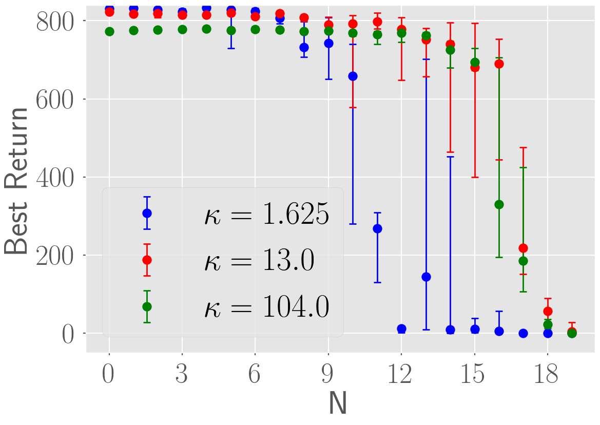
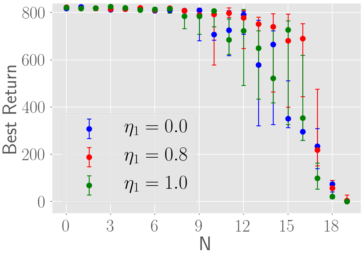
The goal of our experiments is to evaluate the capacity of ISL to perform deep exploration. We test our algorithm in the three deep exploration environments provided by the bsuite benchmark [23] (i.e., Cartpole Swingup, Deep Sea and Deep Sea Stochastic) and compare it against SBEED, UBE [13] and Bootstrap DQN with prior networks (BSP)333We use the implementation provided by [23]. (which provides state of the art results in deep exploration tasks). All three environments have the common quality that exploration is discouraged (due to negative rewards) and positive rewards are only obtained by the agent in states that are hard to reach. We used NNs as function approximators in all cases. Implementation details are included in the Appendix. In appendix 6.9 we also include an ablation study for hyperparameters κ𝜅\kappa, η1subscript𝜂1\eta_{1} and η2subscript𝜂2\eta_{2}.

4.1 Sparse Cartpole Swingup

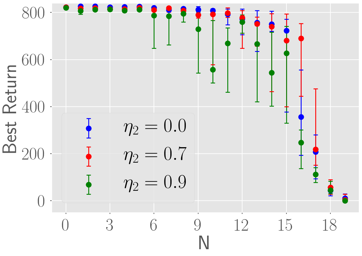
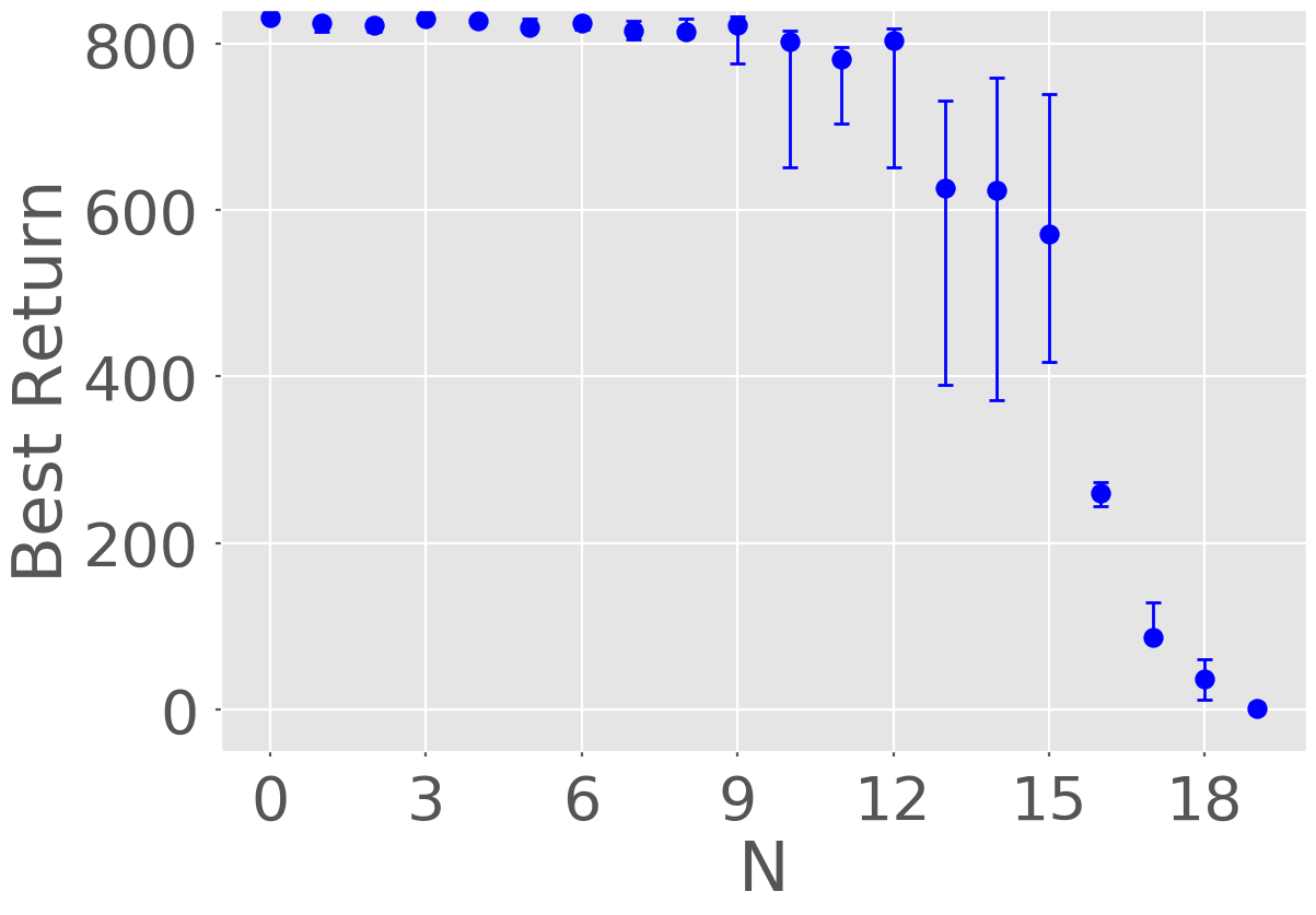
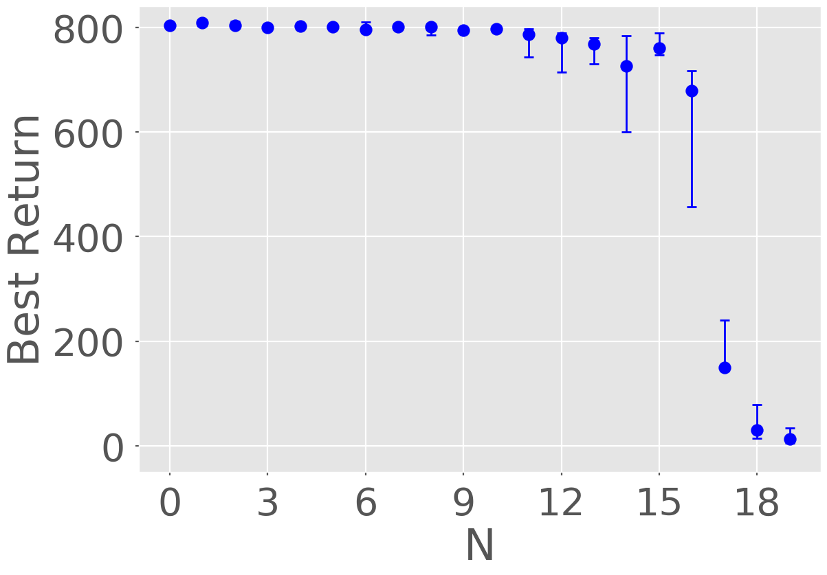
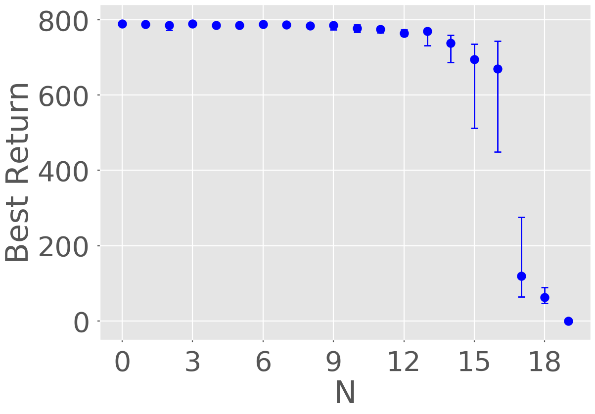
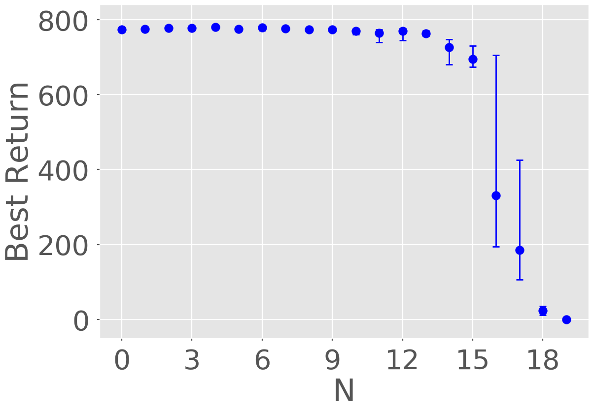
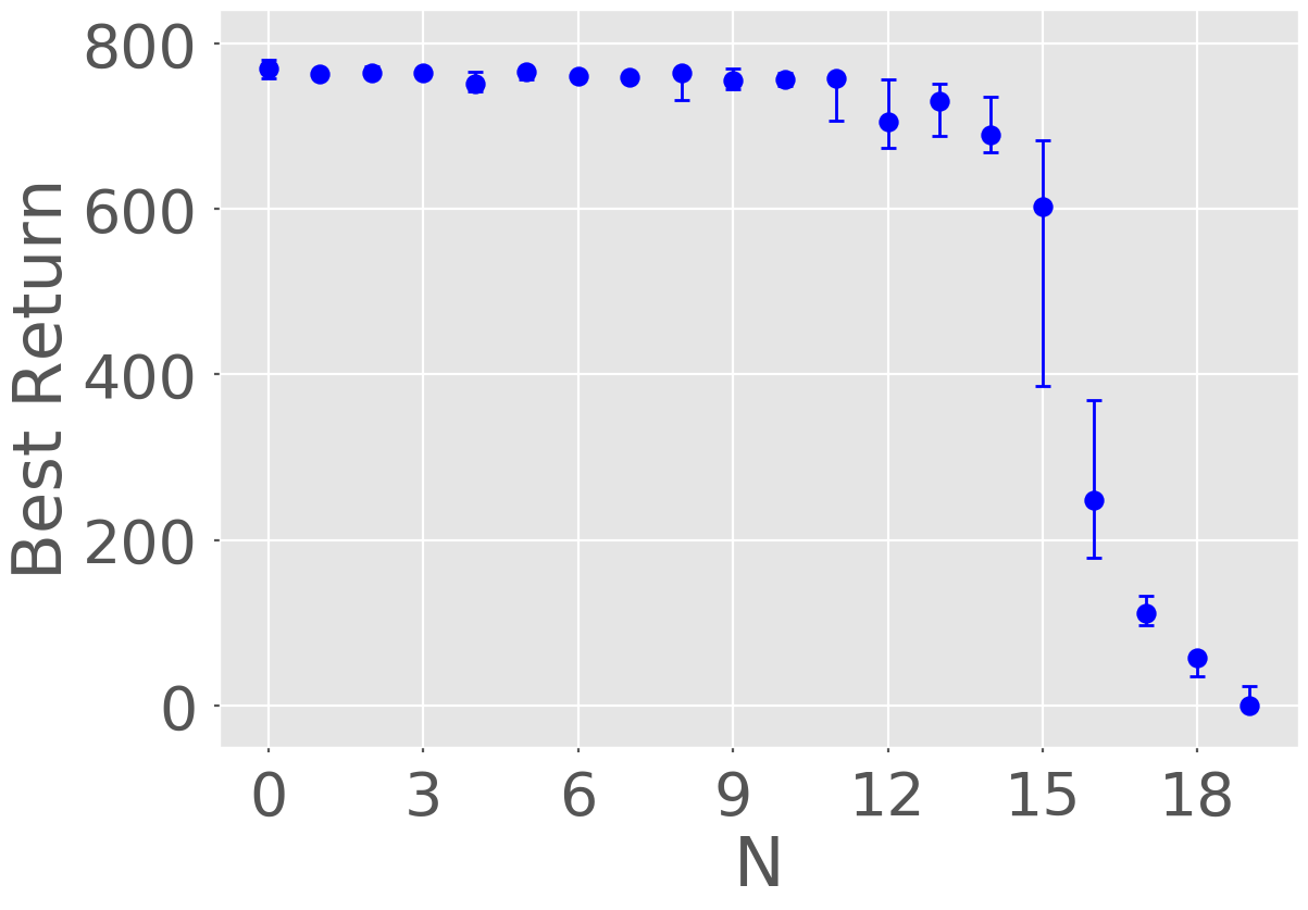
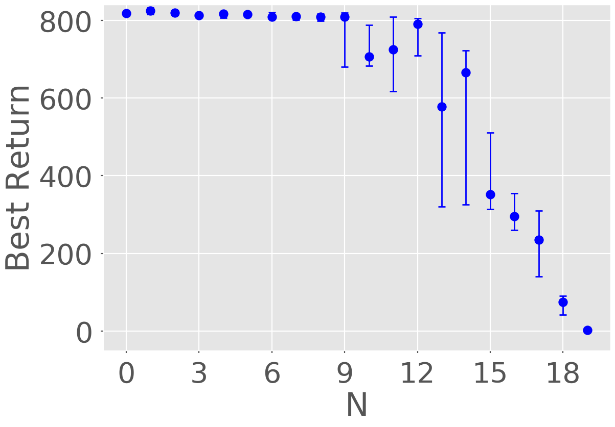
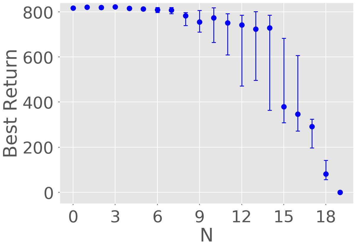
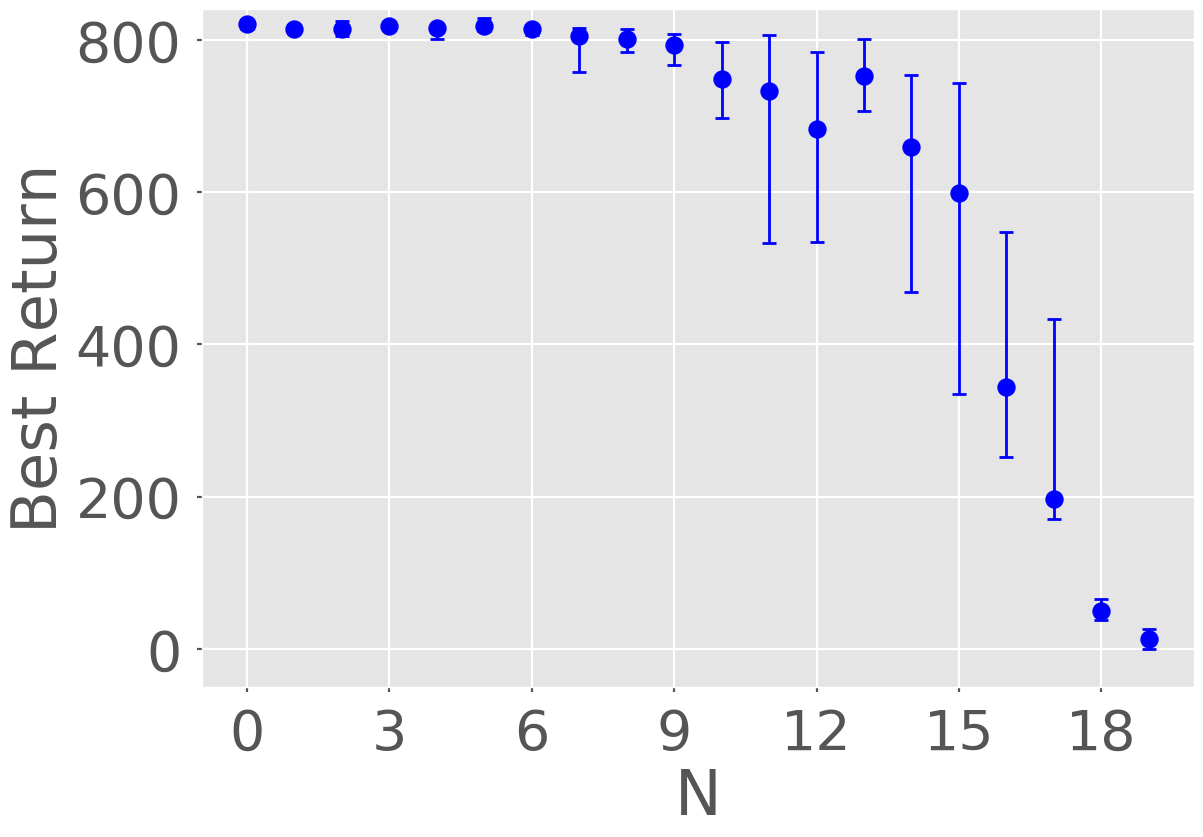
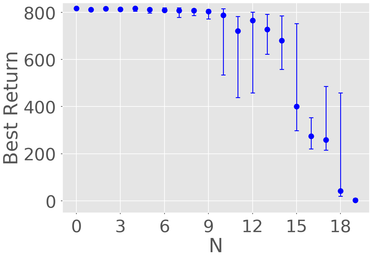
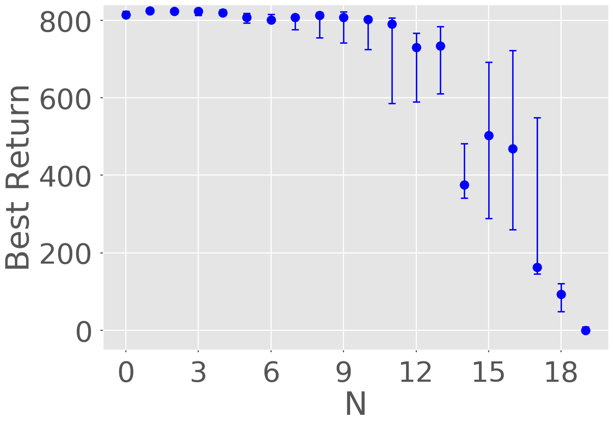
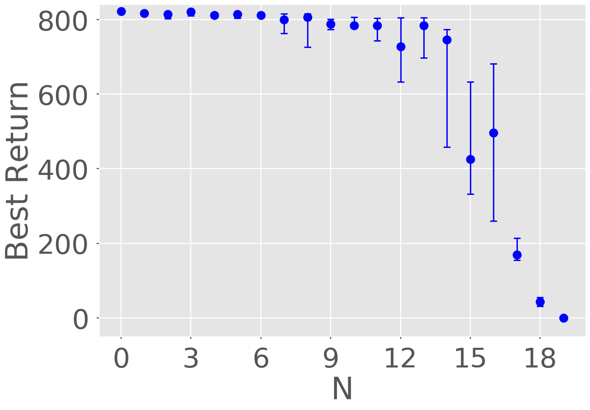
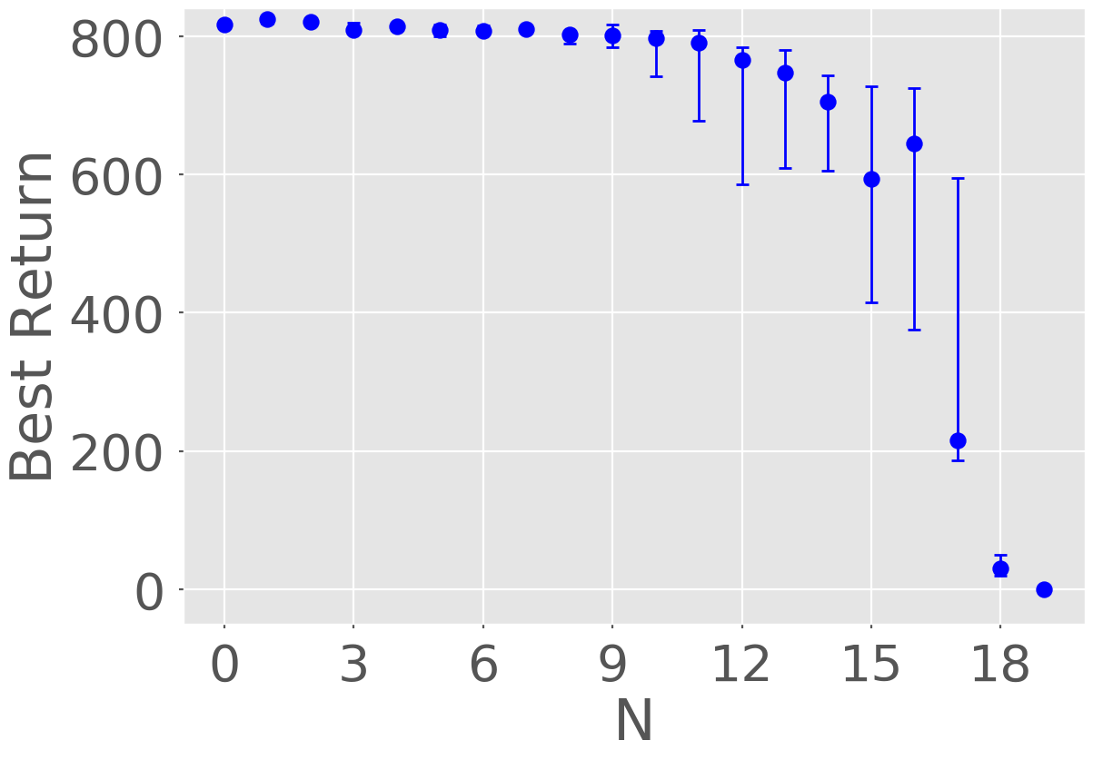
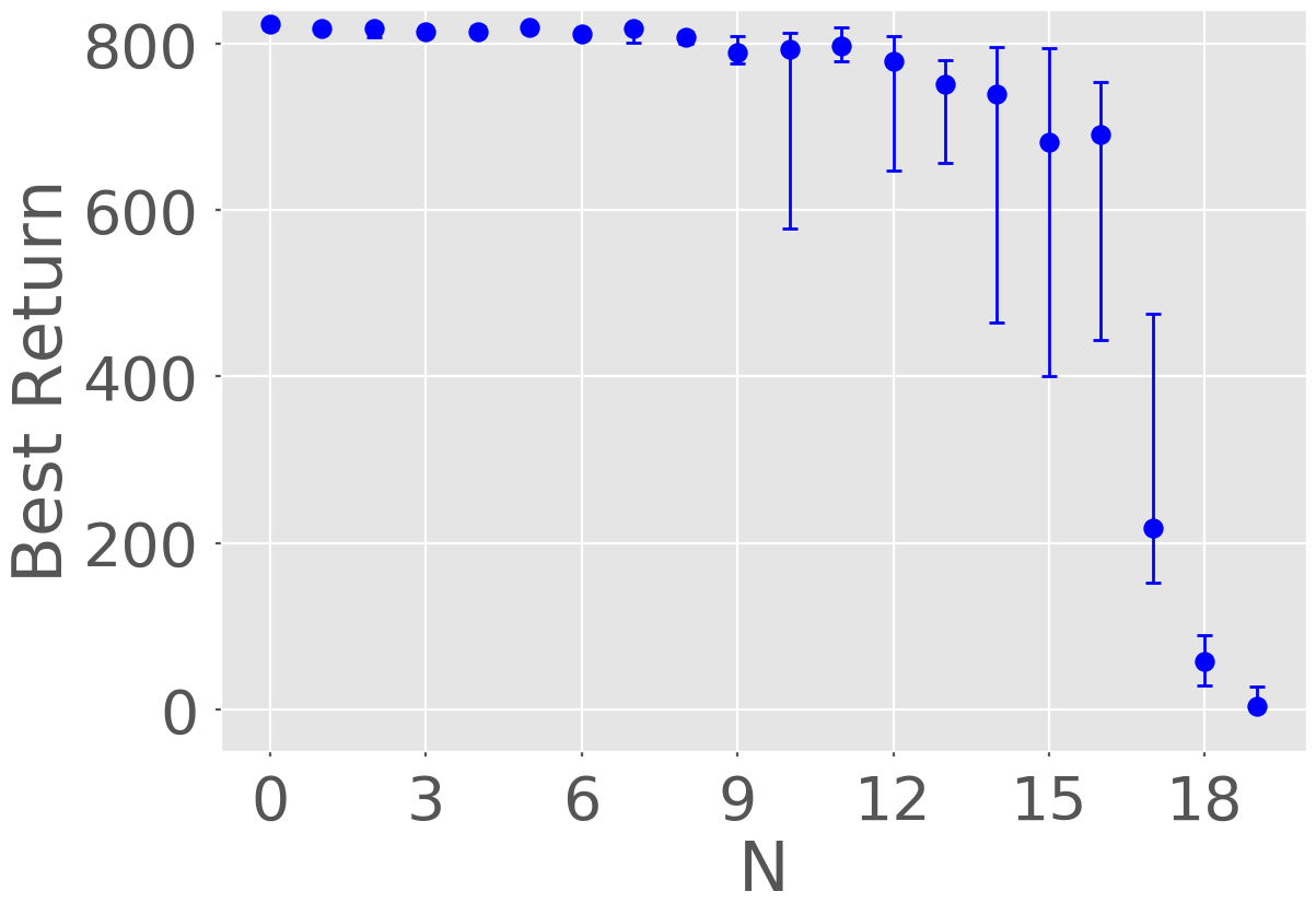
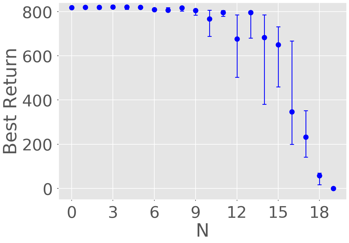
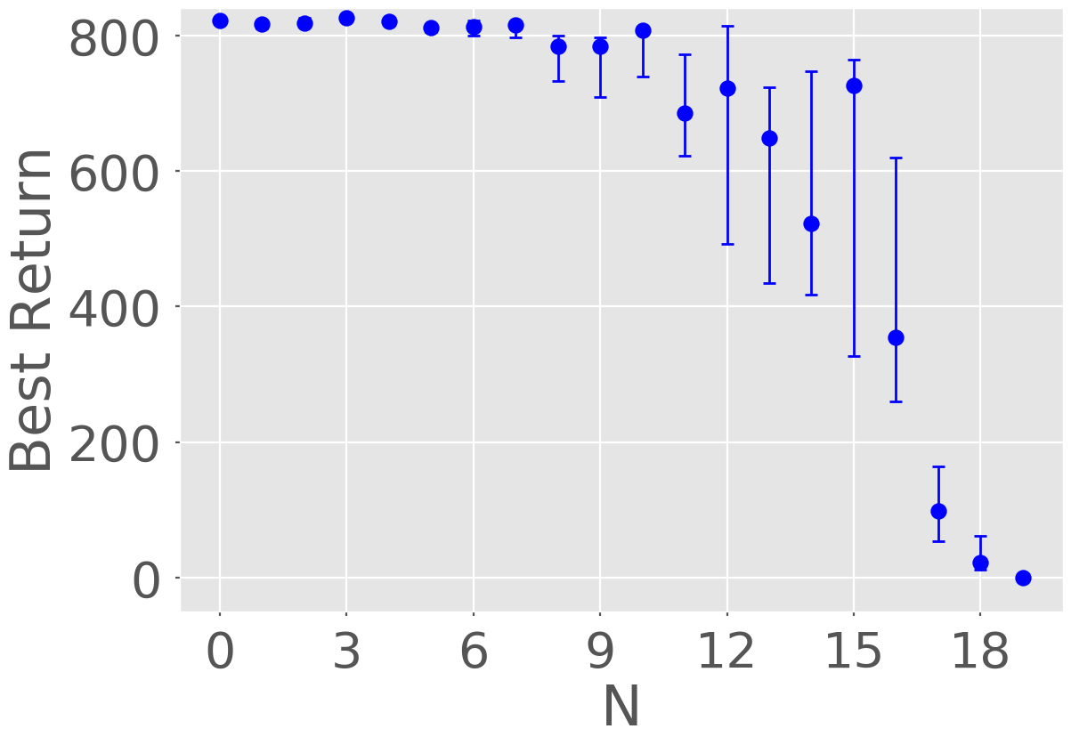
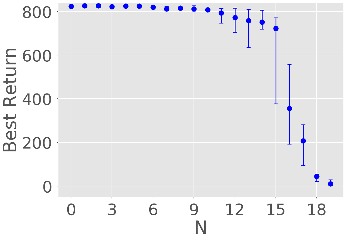
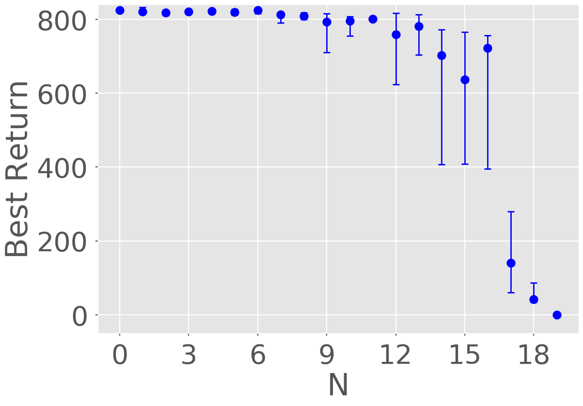
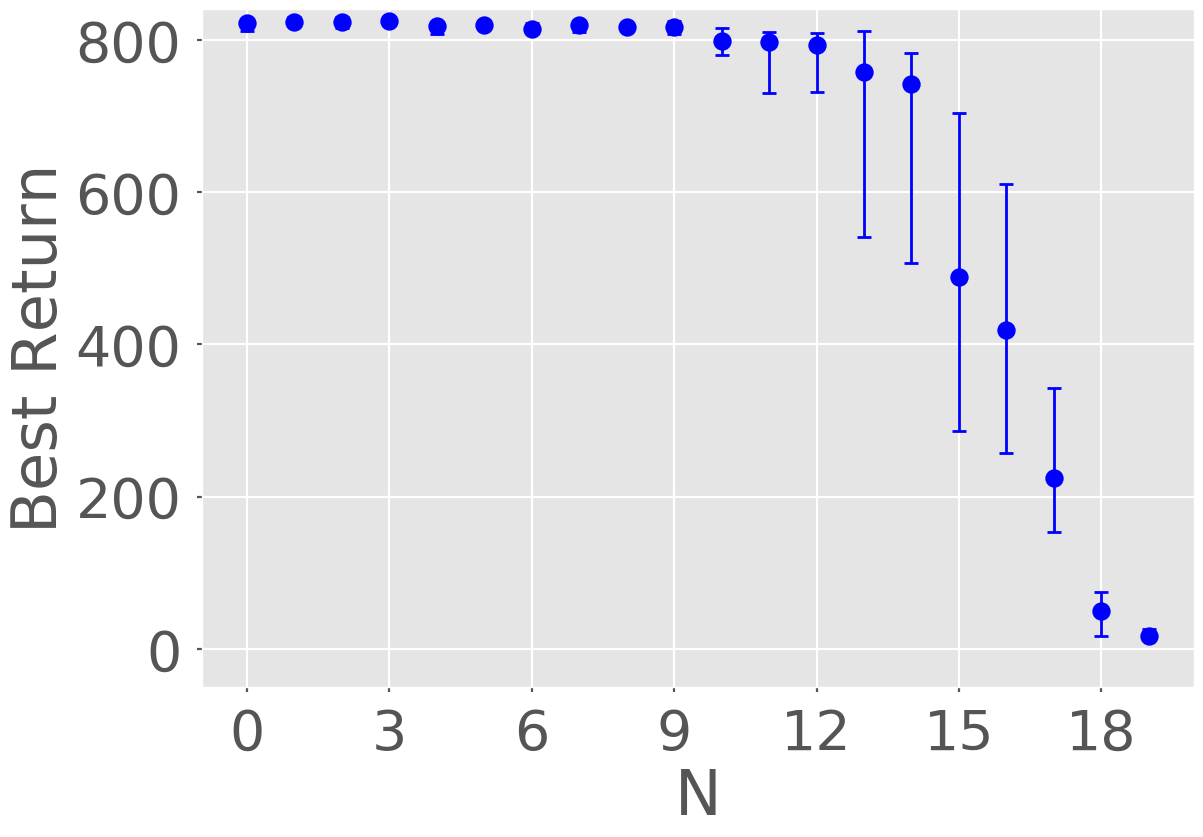
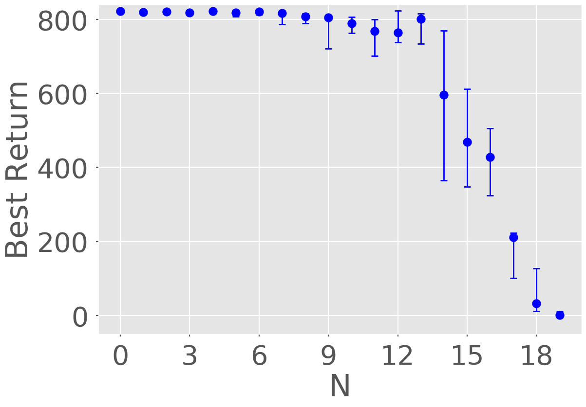
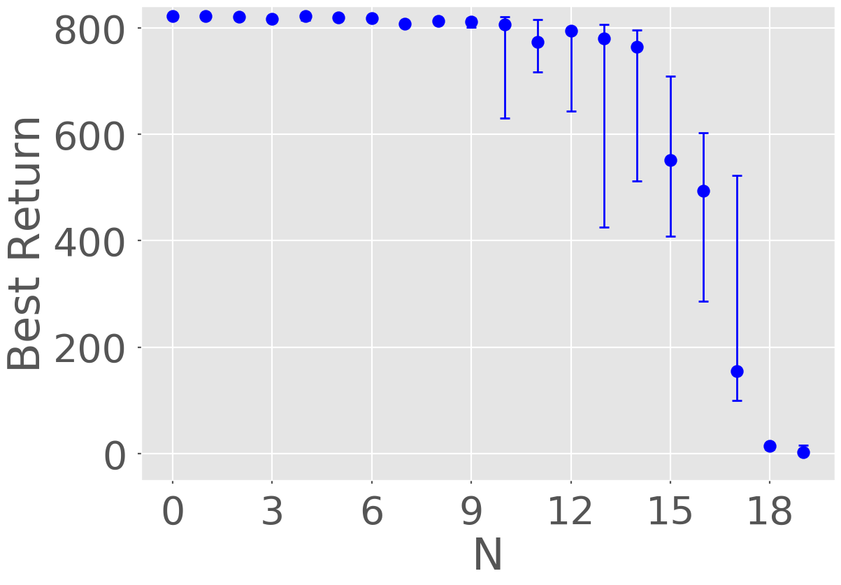
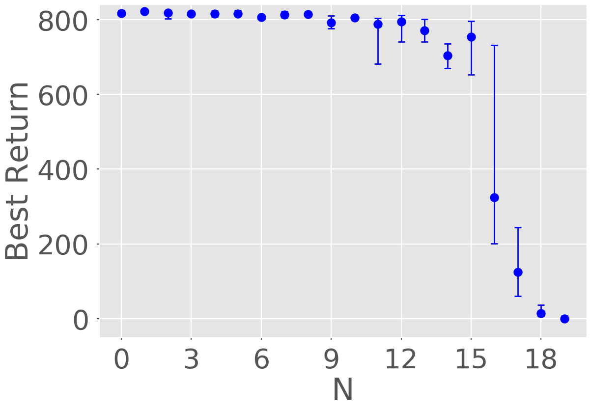
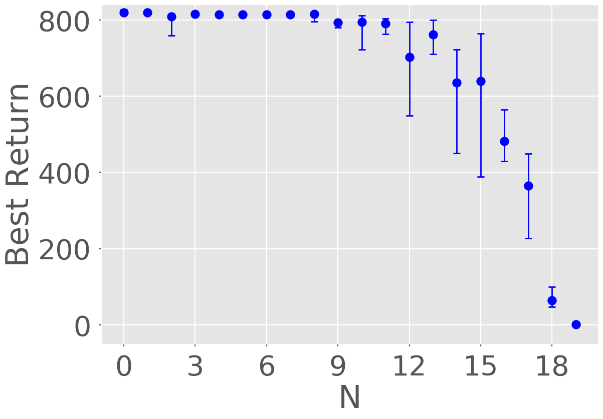
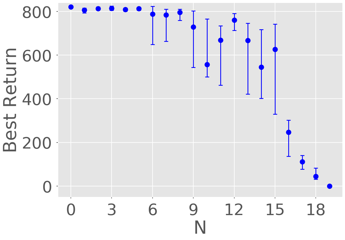
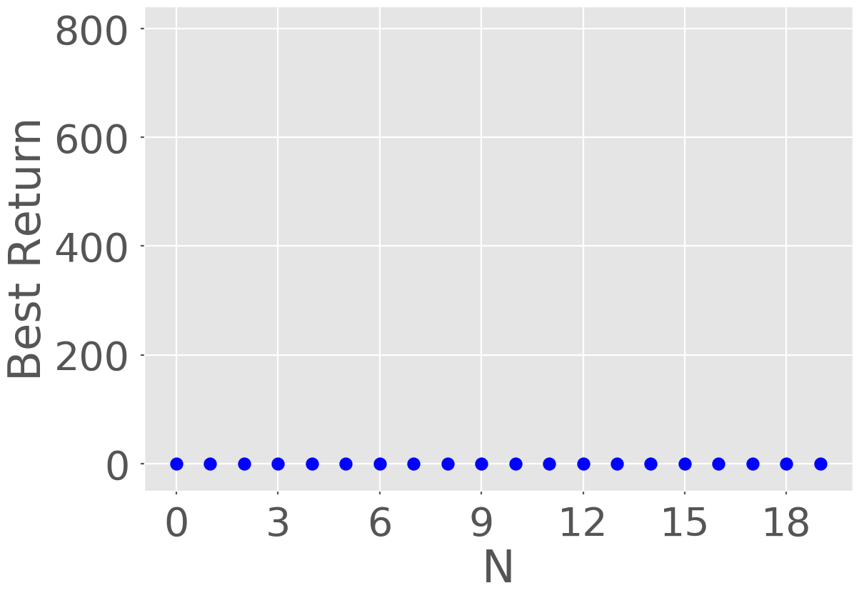
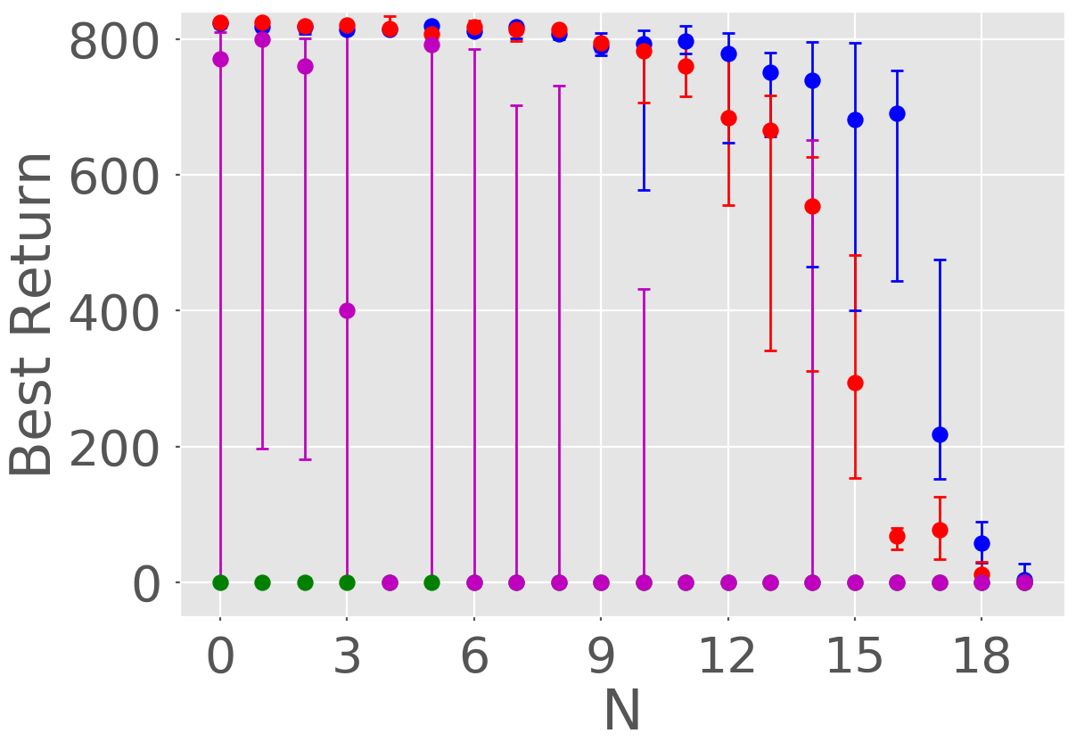
This is the classical cartpole swingup task with the added difficulty that positive rewards are only provided when the pole is ‘almost stabilized’. The action space is {left, stay, right} and the state space is continuous and given by st=(cos(θt),sin(θt),θ˙t,xt,x˙t)subscript𝑠𝑡subscript𝜃𝑡subscript𝜃𝑡subscript˙𝜃𝑡subscript𝑥𝑡subscript˙𝑥𝑡s_{t}=(\cos(\theta_{t}),\sin(\theta_{t}),\dot{\theta}_{t},x_{t},\dot{x}_{t}), where θ𝜃\theta is the angle of the pole and x𝑥x is the position of the cart. The feature that makes this task a challenging exploration task is the reward structure; every move is penalized with a 0.10.1-0.1 reward and a +11+1 is only observed when the cart is ‘almost’ centered and the pole is ‘almost’ upright and stabilized. More specifically, a +11+1 reward is obtained when cos(θ)>N/20𝑐𝑜𝑠𝜃𝑁20cos(\theta)>N/20, |θ˙|<1˙𝜃1|\dot{\theta}|<1 and |x|<1N/20𝑥1𝑁20|x|<1-N/20, where N𝑁N parameterizes the difficulty of the environment. This is an episodic task where each episode ends when the cart moves too far away from the center (|x|>3𝑥3|x|>3) or at 103superscript10310^{3} time-steps, whichever occurs first. We ran each algorithm for 103superscript10310^{3} episodes for ten random seeds. In this benchmark the performance measure is the best return attained during training. The results for N𝑁N from 0 to 19 are shown in figures 1(a). As expected SBEED fails in this task for all values of N𝑁N due to the lack of a mechanism to encourage deep exploration. ISL and BSP find close to optimal policies for all values of N𝑁N up to 10 approximately. However, for higher values of N𝑁N ISL outperforms BSP by a significant margin. For N=19𝑁19N=19 all algorithms fail, however ISL is the only algorithm who can obtain some positive rewards.
Refer to caption
(a) Cartpole swingup
Refer to caption
(b) Deep sea
Refer to caption
(c) Deep sea stochastic
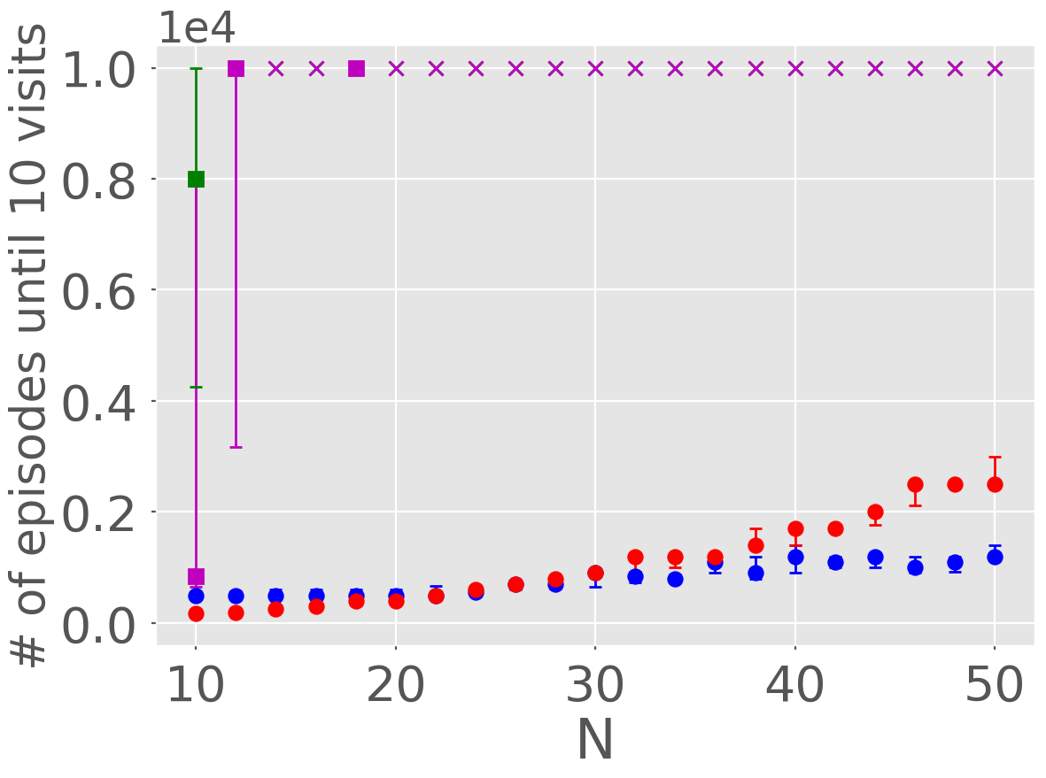
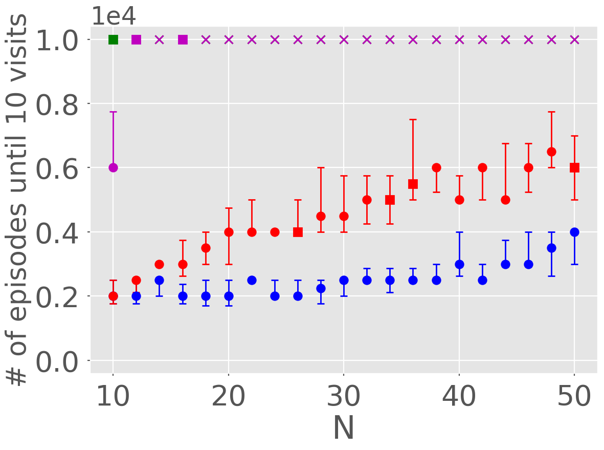
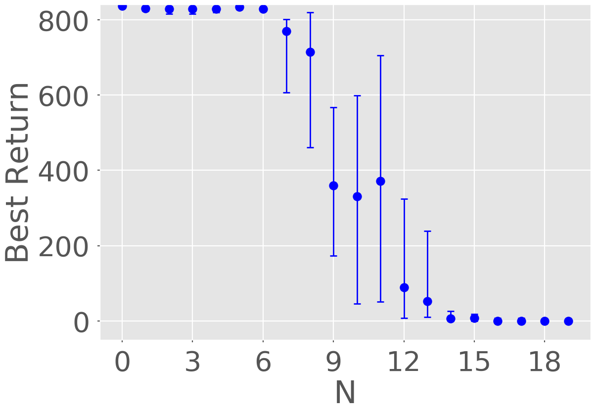
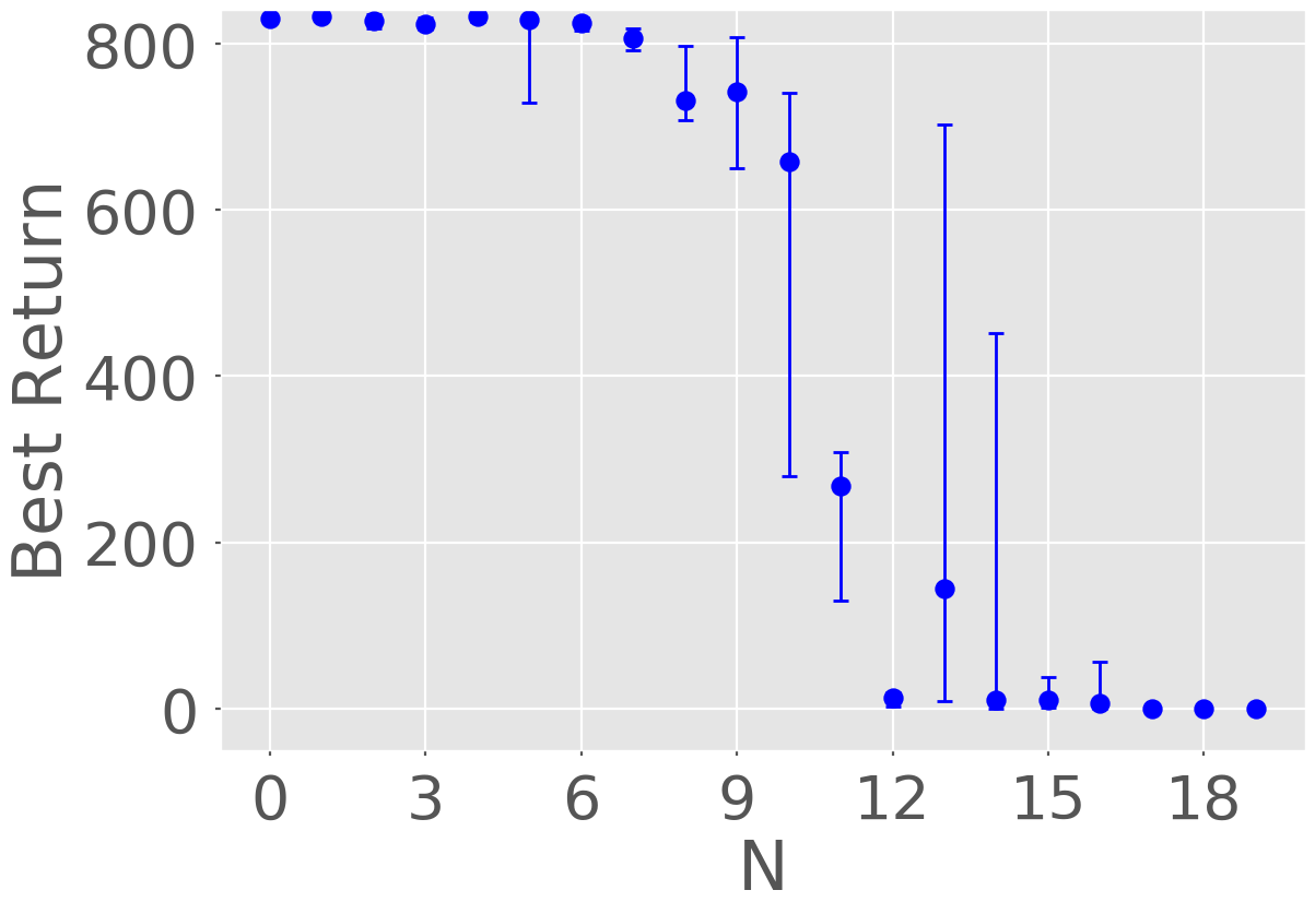
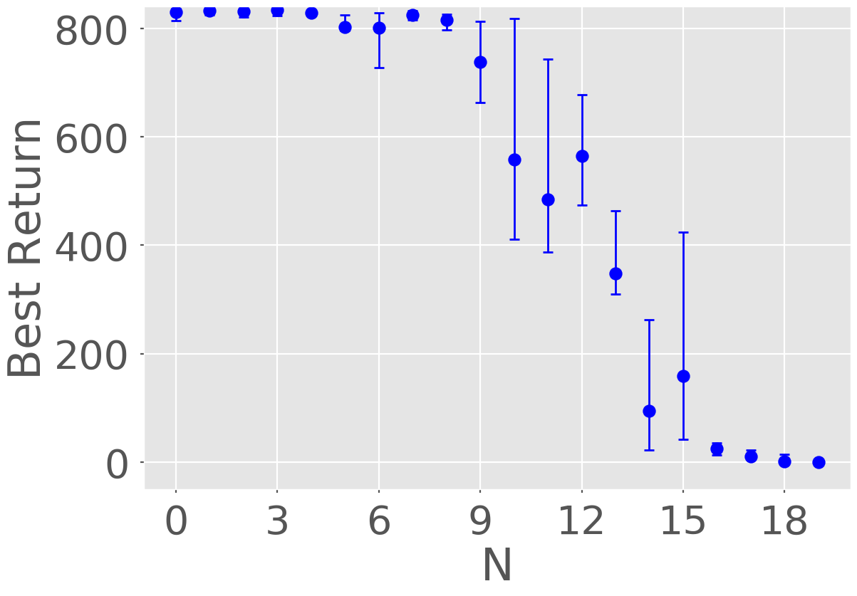
Figure 1: Blue, red, purple and green curves correspond to ISL, BSP, UBE and SBEED, respectively. In all cases we ran 10 experiments with different seeds, the plots show the median and first and third quartiles. In figures 1(b) and 1(c) we used dots are markers when the goal was accomplished (at least 10 visits where made to the desired state) for all seeds, square markers denote that the goal was accomplished for some seeds and the cross markers denote failure for all seeds.

4.2 Deep Sea and Deep Sea Stochastic

Deep Sea is an episodic grid-world type game which consists of an N×N𝑁𝑁N\times N grid with N2superscript𝑁2N^{2} states. The observation encodes the agent’s row and column as a one-hot vector st{0,1}N×Nsubscript𝑠𝑡superscript01𝑁𝑁s_{t}\in\{0,1\}^{N\times N}. The environment has two possible actions {a1,a2}subscript𝑎1subscript𝑎2\{a_{1},a_{2}\} and a mask MBer(0.5)N×Nsimilar-to𝑀Bersuperscript0.5𝑁𝑁M\sim\text{Ber}(0.5)^{N\times N}. The mask maps for every state each action to {left, right}left, right\{\textit{left, right}\}. The agent always starts at the top-left corner and at every step deterministically descends one level and further moves left or right (depending on the chosen action). Every time the agent moves right it gets a 0.01/N0.01𝑁-0.01/N reward, except for the bottom-right state in which case it gets a +11+1, while left moves always receive 00 reward. The game ends after N𝑁N time steps and we ran each algorithm for 104superscript10410^{4} episodes. The optimal strategy of the environment is to always move right in which case the total return would be 0.990.990.99. Note that the parameter N𝑁N parameterizes the difficulty of the game. An important point about this environment is that policies that do not encourage deep exploration take 𝒪(2N)𝒪superscript2𝑁\mathcal{O}(2^{N}) episodes to learn the optimal policy [24], while for policies that explore optimally it takes at best 𝒪(N)𝒪𝑁\mathcal{O}(N) episodes (because the state-action space is of size 𝒪(N2)𝒪superscript𝑁2\mathcal{O}(N^{2}) and at every episode N𝑁N state-action pairs are sampled). The Deep Sea Stochastic environment has the added complexity that transitions and rewards are stochastic. In particular, the reward of the last step of the episode is corrupted with additive Gaussian noise with zero mean and variance equal to 1 and further, agents transition to the right only with 11/N11𝑁1-1/N probability. In these benchmarks the performance measure is the amount of episodes played before the agent visits the goal state for the 10-th time. Hyperparameters were tuned for each of the cases, figures 1(b) and 1(c) show the results. Again SBEED fails at these tasks as expected. In the deterministic case ISL and BSP perform similarly. Note also that while ISL shows linear complexity for all values of N𝑁N, BSP shows linear complexity only for low values of N𝑁N. We clarify that the complexity of BSP could probably be improved for larger values of N𝑁N by enlarging the ensemble size, however note that this would come with an added computational cost since the computational cost of BSP scales linearly with the size of the ensemble. In the stochastic environment ISL performs similarly as it does in the deterministic environment and outperforms BSP for all values of N𝑁N. Note further that ISL is the only algorithm that is able to solve the task for all values of N𝑁N for all seeds.

5 Conclusion

In this paper we provide a novel and original approach to address the problem of deep exploration. We also make an interesting connection with the literature on maximum entropy RL. In contrast to current RL algorithms and deep exploration strategies, where deriving the learning equations and the deep exploration strategies are treated separately, in our approach, both the learning equations and the deep exploration strategy are derived in tandem as the solution to a unique optimization problem. Furthermore, we have introduced a practical way of quantifying uncertainty over q𝑞q estimates that is usable with NNs. We hope this ideas might inspire novel and original research directions.

Broader Impact

We believe the material we present does not introduce any societal or ethical considerations worth mentioning in this section.

References

  • Fox et al. [2016] Roy Fox, Ari Pakman, and Naftali Tishby. Taming the noise in reinforcement learning via soft updates. In Proc. Conference on Uncertainty in Artificial Intelligence, pages 202–211, New York, USA, 2016.
  • Haarnoja et al. [2017] Tuomas Haarnoja, Haoran Tang, Pieter Abbeel, and Sergey Levine. Reinforcement learning with deep energy-based policies. In Proc. International Conference on Machine Learning-Volume 70, pages 1352–1361, Sydney, Australia, 2017.
  • Nachum et al. [2017] Ofir Nachum, Mohammad Norouzi, Kelvin Xu, and Dale Schuurmans. Bridging the gap between value and policy based reinforcement learning. In Proc. Advances in Neural Information Processing Systems, pages 2775–2785, Long Beach, USA, 2017.
  • Haarnoja et al. [2018a] Tuomas Haarnoja, Aurick Zhou, Pieter Abbeel, and Sergey Levine. Soft actor-critic: Off-policy maximum entropy deep reinforcement learning with a stochastic actor. In Proc. International Conference on Machine Learning, pages 1856–1865, Stockholm, Sweden, 2018a.
  • Nachum et al. [2018] Ofir Nachum, Mohammad Norouzi, Kelvin Xu, and Dale Schuurmans. Trust-PCL: An off-policy trust region method for continuous control. arXiv:1707.01891, February 2018.
  • Dai et al. [2018] Bo Dai, Albert Shaw, Lihong Li, Lin Xiao, Niao He, Zhen Liu, Jianshu Chen, and Le Song. SBEED: Convergent reinforcement learning with nonlinear function approximation. In Proc. International Conference on Machine Learning, pages 1133–1142, Stockholm, Sweden, 2018.
  • Haarnoja et al. [2018b] Tuomas Haarnoja, Aurick Zhou, Sehoon Ha, Jie Tan, George Tucker, and Sergey Levine. Learning to walk via deep reinforcement learning. arXiv:1812.11103, 2018b.
  • Mnih et al. [2016] Volodymyr Mnih, Adria Puigdomenech Badia, Mehdi Mirza, Alex Graves, Timothy Lillicrap, Tim Harley, David Silver, and Koray Kavukcuoglu. Asynchronous methods for deep reinforcement learning. In Proc. International Conference on Machine Learning, pages 1928–1937, New York, USA, 2016.
  • Schulman et al. [2015] John Schulman, Sergey Levine, Pieter Abbeel, Michael Jordan, and Philipp Moritz. Trust region policy optimization. In International Conference on Machine Learning, pages 1889–1897, New York, USA, 2015.
  • Schulman et al. [2017] John Schulman, Filip Wolski, Prafulla Dhariwal, Alec Radford, and Oleg Klimov. Proximal policy optimization algorithms. arXiv:1707.06347, August 2017.
  • Stadie et al. [2015] Bradly C Stadie, Sergey Levine, and Pieter Abbeel. Incentivizing exploration in reinforcement learning with deep predictive models. arXiv:1507.00814, 2015.
  • Osband et al. [2016a] Ian Osband, Charles Blundell, Alexander Pritzel, and Benjamin Van Roy. Deep exploration via bootstrapped DQN. In Proc. Advances in neural information processing systems, pages 4026–4034, Barcelona, Spain, 2016a.
  • O’Donoghue et al. [2018] Brendan O’Donoghue, Ian Osband, Remi Munos, and Volodymyr Mnih. The Uncertainty Bellman Equation and Exploration. In International Conference on Machine Learning, pages 3839–3848, Stockholm, Sweden, July 2018.
  • Burda et al. [2018a] Yuri Burda, Harri Edwards, Deepak Pathak, Amos Storkey, Trevor Darrell, and Alexei A Efros. Large-scale study of curiosity-driven learning. arXiv:1808.04355, 2018a.
  • Osband et al. [2018] Ian Osband, John Aslanides, and Albin Cassirer. Randomized prior functions for deep reinforcement learning. In Proc. Advances in Neural Information Processing Systems, pages 8617–8629, Montréal, Canada, 2018.
  • Cassano et al. [2019] Lucas Cassano, Sulaiman A. Alghunaim, and Ali H. Sayed. Team policy learning for multi-agent reinforcement learning. In Proc. IEEE International Conference on Acoustics, Speech and Signal Processing (ICASSP), pages 3062–3066, Brighton, UK, May 2019.
  • Bellemare et al. [2016] Marc Bellemare, Sriram Srinivasan, Georg Ostrovski, Tom Schaul, David Saxton, and Remi Munos. Unifying count-based exploration and intrinsic motivation. In Advances in neural information processing systems, pages 1471–1479, 2016.
  • Ostrovski et al. [2017] Georg Ostrovski, Marc G Bellemare, Aäron van den Oord, and Rémi Munos. Count-based exploration with neural density models. In Proc of International Conference on Machine Learning, pages 2721–2730, 2017.
  • Houthooft et al. [2016] Rein Houthooft, Xi Chen, Yan Duan, John Schulman, Filip De Turck, and Pieter Abbeel. Vime: Variational information maximizing exploration. In Advances in Neural Information Processing Systems, pages 1109–1117, 2016.
  • Pathak et al. [2017] Deepak Pathak, Pulkit Agrawal, Alexei A Efros, and Trevor Darrell. Curiosity-driven exploration by self-supervised prediction. In Proc. of International Conference on Machine Learning-Volume 70, pages 2778–2787, 2017.
  • Burda et al. [2018b] Yuri Burda, Harrison Edwards, Amos Storkey, and Oleg Klimov. Exploration by random network distillation. arXiv:1810.12894, 2018b.
  • Puterman [2014] Martin L Puterman. Markov Decision Processes.: Discrete Stochastic Dynamic Programming. Wiley, NY, 2014.
  • Osband et al. [2019] Ian Osband, Yotam Doron, Matteo Hessel, John Aslanides, Eren Sezener, Andre Saraiva, Katrina McKinney, Tor Lattimore, Csaba Szepezvari, Satinder Singh, Benjamin Van Roy, Richard Sutton, David Silver, and Hado Van Hasselt. Behaviour suite for reinforcement learning. arXiv:1908.03568, August 2019.
  • Osband et al. [2016b] Ian Osband, Benjamin Van Roy, and Zheng Wen. Generalization and exploration via randomized value functions. In International Conference on International Conference on Machine Learning-Volume 48, pages 2377–2386, June 2016b.

6 Appendix

6.1 Proof of Lemma 1

In the proof we assume that the actions are ordered following the lemma’s assumption. By definition, the KL divergence is given by:

DKL(usπ(q~))subscript𝐷𝐾𝐿superscriptsubscript𝑢𝑠𝜋~𝑞\displaystyle D_{KL}(u_{s}^{\pi}(\widetilde{q})) =q~usπ(q~)log(usπ(q~)us(q~))𝑑q~absentsubscript~𝑞superscriptsubscript𝑢𝑠𝜋~𝑞superscriptsubscript𝑢𝑠𝜋~𝑞superscriptsubscript𝑢𝑠~𝑞differential-d~𝑞\displaystyle=\int_{\widetilde{q}}u_{s}^{\pi}(\widetilde{q})\log\left(\frac{u_{s}^{\pi}(\widetilde{q})}{u_{s}^{\bullet}(\widetilde{q})}\right)d\widetilde{q}
=(b)aπ(a|s)q~d(s,a)(q~)log(aπ(a|s)d(s,a)(q~))𝑑q~+log(A)superscript𝑏absentsubscript𝑎𝜋conditional𝑎𝑠subscript~𝑞subscript𝑑𝑠𝑎~𝑞subscriptsuperscript𝑎𝜋conditionalsuperscript𝑎𝑠subscript𝑑𝑠superscript𝑎~𝑞differential-d~𝑞subscript𝐴\displaystyle\stackrel{{\scriptstyle(b)}}{{=}}\sum_{a}\pi(a|s)\int_{\widetilde{q}}d_{(s,a)}(\widetilde{q})\log\left(\sum_{a^{\prime}}\pi(a^{\prime}|s)d_{(s,a^{\prime})}(\widetilde{q})\right)d\widetilde{q}+\log(\ell_{A}) (19)

where in (b)𝑏(b) we used (4). Note that since δπ(s)superscript𝛿𝜋𝑠\delta^{\pi}(s) is a piecewise constant distribution, the integral in (19) has the following closed form expression:

q~d(s,aj)(q~)log(aπ(a|s)d(s,a)(q~))𝑑q~=jj(2j)1log(aπ(a|s)d(s,a)(q~))𝑑q~subscript~𝑞subscript𝑑𝑠subscript𝑎𝑗~𝑞subscriptsuperscript𝑎𝜋conditionalsuperscript𝑎𝑠subscript𝑑𝑠superscript𝑎~𝑞differential-d~𝑞superscriptsubscriptsubscript𝑗subscript𝑗superscript2subscript𝑗1subscriptsuperscript𝑎𝜋conditionalsuperscript𝑎𝑠subscript𝑑𝑠superscript𝑎~𝑞differential-d~𝑞\displaystyle\int_{\widetilde{q}}d_{(s,a_{j})}(\widetilde{q})\log\left(\sum_{a^{\prime}}\pi(a^{\prime}|s)d_{(s,a^{\prime})}(\widetilde{q})\right)d\widetilde{q}=\int_{-\ell_{j}}^{\ell_{j}}(2\ell_{j})^{-1}\log\left(\sum_{a^{\prime}}\pi(a^{\prime}|s)d_{(s,a^{\prime})}(\widetilde{q})\right)d\widetilde{q}
=j1j1jlog(aπ(a|s)d(s,a)(q~))𝑑q~+j10j1log(aπ(a|s)d(s,a)(q~))𝑑q~absentsuperscriptsubscript𝑗1superscriptsubscriptsubscript𝑗1subscript𝑗subscriptsuperscript𝑎𝜋conditionalsuperscript𝑎𝑠subscript𝑑𝑠superscript𝑎~𝑞differential-d~𝑞superscriptsubscript𝑗1superscriptsubscript0subscript𝑗1subscriptsuperscript𝑎𝜋conditionalsuperscript𝑎𝑠subscript𝑑𝑠superscript𝑎~𝑞differential-d~𝑞\displaystyle=\ell_{j}^{-1}\int_{{\ell_{j-1}}}^{\ell_{j}}\log\left(\sum_{a^{\prime}}\pi(a^{\prime}|s)d_{(s,a^{\prime})}(\widetilde{q})\right)d\widetilde{q}+\ell_{j}^{-1}\int_{0}^{\ell_{j-1}}\log\left(\sum_{a^{\prime}}\pi(a^{\prime}|s)d_{(s,a^{\prime})}(\widetilde{q})\right)d\widetilde{q}
=jj1jlog(b=0Ajπ(Ab|s)Ab1)+j10j1log(aπ(a|s)d(s,a)(b))𝑑q~absentsubscript𝑗subscript𝑗1subscript𝑗superscriptsubscript𝑏0𝐴𝑗𝜋𝐴conditional𝑏𝑠superscriptsubscript𝐴𝑏1superscriptsubscript𝑗1superscriptsubscript0subscript𝑗1subscriptsuperscript𝑎𝜋conditionalsuperscript𝑎𝑠subscript𝑑𝑠superscript𝑎𝑏differential-d~𝑞\displaystyle=\frac{\ell_{j}-\ell_{j-1}}{\ell_{j}}\log\left(\sum_{b=0}^{A-j}\pi(A-b|s)\ell_{A-b}^{-1}\right)+\ell_{j}^{-1}\int_{0}^{\ell_{j-1}}\log\left(\sum_{a^{\prime}}\pi(a^{\prime}|s)d_{(s,a^{\prime})}(b)\right)d\widetilde{q}
=n=1jnn1jlog(b=nAπ(b|s)b)absentsuperscriptsubscript𝑛1𝑗subscript𝑛subscript𝑛1subscript𝑗superscriptsubscript𝑏𝑛𝐴𝜋conditional𝑏𝑠subscript𝑏\displaystyle=\sum_{n=1}^{j}\frac{\ell_{n}-\ell_{n-1}}{\ell_{j}}\log\left(\sum_{b=n}^{A}\frac{\pi(b|s)}{\ell_{b}}\right) (20)

Combining (19) and (20) we get:

k=1Aπ(ak|s)kn=1k(nn1)log[b=nAπ(b|s)Ab]superscriptsubscript𝑘1𝐴𝜋conditionalsubscript𝑎𝑘𝑠subscript𝑘superscriptsubscript𝑛1𝑘subscript𝑛subscript𝑛1superscriptsubscript𝑏𝑛𝐴𝜋conditional𝑏𝑠subscript𝐴subscript𝑏\displaystyle\sum_{k=1}^{A}\frac{\pi(a_{k}|s)}{\ell_{k}}\sum_{n=1}^{k}(\ell_{n}-\ell_{n-1})\log\left[\sum_{b=n}^{A}\frac{\pi(b|s)\ell_{A}}{\ell_{b}}\right] (21)

Rearranging the terms in (21) we get:

DKL(usπ(q~))=n=1A(nn1)(k=nAπ(ak|s)k)log[b=nAπ(b|s)Ab]subscript𝐷𝐾𝐿superscriptsubscript𝑢𝑠𝜋~𝑞superscriptsubscript𝑛1𝐴subscript𝑛subscript𝑛1superscriptsubscript𝑘𝑛𝐴𝜋conditionalsubscript𝑎𝑘𝑠subscript𝑘superscriptsubscript𝑏𝑛𝐴𝜋conditional𝑏𝑠subscript𝐴subscript𝑏\displaystyle D_{KL}(u_{s}^{\pi}(\widetilde{q}))=\sum_{n=1}^{A}(\ell_{n}-\ell_{n-1})\left(\sum_{k=n}^{A}\frac{\pi(a_{k}|s)}{\ell_{k}}\right)\log\left[\sum_{b=n}^{A}\frac{\pi(b|s)\ell_{A}}{\ell_{b}}\right] (22)

6.2 Proof Lemma 2

We start proving that for any action ajsubscript𝑎𝑗a_{j} that is Pareto dominated by another action aisubscript𝑎𝑖a_{i} it must be the case that π(aj|s)=0superscript𝜋conditionalsubscript𝑎𝑗𝑠0\pi^{\star}(a_{j}|s)=0. We now present an assumption to make notation simpler.

Assumption 2.

In this section we assume without loss of generality that actions are ordered such that i>ji>jiffsubscript𝑖subscript𝑗𝑖𝑗\ell_{i}>\ell_{j}\iff i>j.

We prove the lemma by contradiction. Assume that there is a uc𝑢𝑐uc-optimal policy π1subscript𝜋1\pi_{1} for which π1(aj|s1)>0subscript𝜋1conditionalsubscript𝑎𝑗subscript𝑠10\pi_{1}(a_{j}|s_{1})>0. We now define policy π2subscript𝜋2\pi_{2} as:

π2(a|s)={π1(a|s)αif (s,a)=(s1,aj)π1(a|s)+αif (s,a)=(s1,ai)π1(a|s)elsesubscript𝜋2conditional𝑎𝑠casessubscript𝜋1conditional𝑎𝑠𝛼if (s,a)=(s1,aj)otherwisesubscript𝜋1conditional𝑎𝑠𝛼if (s,a)=(s1,ai)otherwisesubscript𝜋1conditional𝑎𝑠elseotherwise\displaystyle\pi_{2}(a|s)=\begin{cases}\pi_{1}(a|s)-\alpha\hskip 14.22636pt\textrm{if $(s,a)=(s_{1},a_{j})$}\\ \pi_{1}(a|s)+\alpha\hskip 14.22636pt\textrm{if $(s,a)=(s_{1},a_{i})$}\\ \pi_{1}(a|s)\hskip 28.45274pt\textrm{else}\end{cases} (23)

where 0<α<π1(a|s)0𝛼subscript𝜋1conditional𝑎𝑠0<\alpha<\pi_{1}(a|s). We show that vπ2(s1)α|α=0>0evaluated-atsuperscript𝑣subscript𝜋2subscript𝑠1𝛼𝛼00\frac{\partial v^{\pi_{2}}(s_{1})}{\partial\alpha}\big{|}_{\alpha=0}>0 and hence vπ2(s1)>vπ1(s1)superscript𝑣subscript𝜋2subscript𝑠1superscript𝑣subscript𝜋1subscript𝑠1v^{\pi_{2}}(s_{1})>v^{\pi_{1}}(s_{1}) for a small enough α>0𝛼0\alpha>0, which contradicts the claim that π1subscript𝜋1\pi_{1} is a uc𝑢𝑐uc-optimal policy.

vπ2(s1)α|α=0evaluated-atsuperscript𝑣subscript𝜋2subscript𝑠1𝛼𝛼0\displaystyle\frac{\partial v^{\pi_{2}}(s_{1})}{\partial\alpha}\bigg{|}_{\alpha=0} =vπ2(s1)π1(aj|s1)π1(aj|s1)α|α=0+vπ2(s1)π1(ai|s1)π1(ai|s1)α|α=0absentevaluated-atsuperscript𝑣subscript𝜋2subscript𝑠1subscript𝜋1conditionalsubscript𝑎𝑗subscript𝑠1subscript𝜋1conditionalsubscript𝑎𝑗subscript𝑠1𝛼𝛼0evaluated-atsuperscript𝑣subscript𝜋2subscript𝑠1subscript𝜋1conditionalsubscript𝑎𝑖subscript𝑠1subscript𝜋1conditionalsubscript𝑎𝑖subscript𝑠1𝛼𝛼0\displaystyle=\frac{\partial v^{\pi_{2}}(s_{1})}{\partial\pi_{1}(a_{j}|s_{1})}\frac{\partial\pi_{1}(a_{j}|s_{1})}{\partial\alpha}\bigg{|}_{\alpha=0}+\frac{\partial v^{\pi_{2}}(s_{1})}{\partial\pi_{1}(a_{i}|s_{1})}\frac{\partial\pi_{1}(a_{i}|s_{1})}{\partial\alpha}\bigg{|}_{\alpha=0}
=vπ2(s1)π1(ai|s1)vπ2(s1)π1(aj|s1)absentsuperscript𝑣subscript𝜋2subscript𝑠1subscript𝜋1conditionalsubscript𝑎𝑖subscript𝑠1superscript𝑣subscript𝜋2subscript𝑠1subscript𝜋1conditionalsubscript𝑎𝑗subscript𝑠1\displaystyle=\frac{\partial v^{\pi_{2}}(s_{1})}{\partial\pi_{1}(a_{i}|s_{1})}-\frac{\partial v^{\pi_{2}}(s_{1})}{\partial\pi_{1}(a_{j}|s_{1})}
=q^π2(s,ai)q^π2(s,aj)>0 (due to Pareto assumption)+κ(DKL(us1π2(q~))π1(aj|s1)DKL(us1π2(q~))π1(ai|s1))absentsubscriptsuperscript^𝑞subscript𝜋2𝑠subscript𝑎𝑖superscript^𝑞subscript𝜋2𝑠subscript𝑎𝑗absent0 (due to Pareto assumption)𝜅subscript𝐷𝐾𝐿superscriptsubscript𝑢subscript𝑠1subscript𝜋2~𝑞subscript𝜋1conditionalsubscript𝑎𝑗subscript𝑠1subscript𝐷𝐾𝐿superscriptsubscript𝑢subscript𝑠1subscript𝜋2~𝑞subscript𝜋1conditionalsubscript𝑎𝑖subscript𝑠1\displaystyle=\underbrace{\widehat{q}^{\pi_{2}}(s,a_{i})-\widehat{q}^{\pi_{2}}(s,a_{j})}_{>0\textrm{ (due to Pareto assumption)}}+\kappa\left(\frac{\partial D_{KL}(u_{s_{1}}^{\pi_{2}}(\widetilde{q}))}{\partial\pi_{1}(a_{j}|s_{1})}-\frac{\partial D_{KL}(u_{s_{1}}^{\pi_{2}}(\widetilde{q}))}{\partial\pi_{1}(a_{i}|s_{1})}\right) (24)

Using (22) we get the following expression for the gradient of the KL term:

DKL(usπ(q~))π(aj|s)subscript𝐷𝐾𝐿superscriptsubscript𝑢𝑠𝜋~𝑞𝜋conditionalsubscript𝑎𝑗𝑠\displaystyle\frac{\partial D_{KL}(u_{s}^{\pi}(\widetilde{q}))}{\partial\pi(a_{j}|s)} =b=1j(bb1)jlog(c=bAπ(c|s)c)+j1b=1j(bb1)absentsuperscriptsubscript𝑏1𝑗subscript𝑏subscript𝑏1subscript𝑗superscriptsubscript𝑐𝑏𝐴𝜋conditional𝑐𝑠subscript𝑐superscriptsubscript𝑗1superscriptsubscript𝑏1𝑗subscript𝑏subscript𝑏1\displaystyle=\sum_{b=1}^{j}\frac{(\ell_{b}-\ell_{b-1})}{\ell_{j}}\log\left(\sum_{c=b}^{A}\frac{\pi(c|s)}{\ell_{c}}\right)+\ell_{j}^{-1}\sum_{b=1}^{j}(\ell_{b}-\ell_{b-1})
=b=1j(bb1)jlog(c=bAπ(c|s)c)+1absentsuperscriptsubscript𝑏1𝑗subscript𝑏subscript𝑏1subscript𝑗superscriptsubscript𝑐𝑏𝐴𝜋conditional𝑐𝑠subscript𝑐1\displaystyle=\sum_{b=1}^{j}\frac{(\ell_{b}-\ell_{b-1})}{\ell_{j}}\log\left(\sum_{c=b}^{A}\frac{\pi(c|s)}{\ell_{c}}\right)+1 (25)

Combining (6.2) and (24) we get:

DKL(us1π2(q~))π1(aj|s1)DKL(us1π2(q~))π1(ai|s1)=b=1j(bb1)jlog(c=bAπ(c|s)c)subscript𝐷𝐾𝐿superscriptsubscript𝑢subscript𝑠1subscript𝜋2~𝑞subscript𝜋1conditionalsubscript𝑎𝑗subscript𝑠1subscript𝐷𝐾𝐿superscriptsubscript𝑢subscript𝑠1subscript𝜋2~𝑞subscript𝜋1conditionalsubscript𝑎𝑖subscript𝑠1superscriptsubscript𝑏1𝑗subscript𝑏subscript𝑏1subscript𝑗superscriptsubscript𝑐𝑏𝐴𝜋conditional𝑐𝑠subscript𝑐\displaystyle\frac{\partial D_{KL}(u_{s_{1}}^{\pi_{2}}(\widetilde{q}))}{\partial\pi_{1}(a_{j}|s_{1})}-\frac{\partial D_{KL}(u_{s_{1}}^{\pi_{2}}(\widetilde{q}))}{\partial\pi_{1}(a_{i}|s_{1})}=\sum_{b=1}^{j}\frac{(\ell_{b}-\ell_{b-1})}{\ell_{j}}\log\left(\sum_{c=b}^{A}\frac{\pi(c|s)}{\ell_{c}}\right)
b=1i(bb1)ilog(c=bAπ(c|s)c)superscriptsubscript𝑏1𝑖subscript𝑏subscript𝑏1subscript𝑖superscriptsubscript𝑐𝑏𝐴𝜋conditional𝑐𝑠subscript𝑐\displaystyle\hskip 142.26378pt-\sum_{b=1}^{i}\frac{(\ell_{b}-\ell_{b-1})}{\ell_{i}}\log\left(\sum_{c=b}^{A}\frac{\pi(c|s)}{\ell_{c}}\right)
=b=1j(bb1)(ij)jilog(c=bAπ(c|s)c)b=j+1i(bb1)ilog(c=bAπ(c|s)c)absentsuperscriptsubscript𝑏1𝑗subscript𝑏subscript𝑏1subscript𝑖subscript𝑗subscript𝑗subscript𝑖superscriptsubscript𝑐𝑏𝐴𝜋conditional𝑐𝑠subscript𝑐superscriptsubscript𝑏𝑗1𝑖subscript𝑏subscript𝑏1subscript𝑖superscriptsubscript𝑐𝑏𝐴𝜋conditional𝑐𝑠subscript𝑐\displaystyle=\sum_{b=1}^{j}\frac{(\ell_{b}-\ell_{b-1})(\ell_{i}-\ell_{j})}{\ell_{j}\ell_{i}}\log\left(\sum_{c=b}^{A}\frac{\pi(c|s)}{\ell_{c}}\right)-\sum_{b=j+1}^{i}\frac{(\ell_{b}-\ell_{b-1})}{\ell_{i}}\log\left(\sum_{c=b}^{A}\frac{\pi(c|s)}{\ell_{c}}\right)
>(a)b=1j(bb1)(ij)jilog(c=jAπ(c|s)c)b=j+1i(bb1)ilog(c=jAπ(c|s)c)superscript𝑎absentsuperscriptsubscript𝑏1𝑗subscript𝑏subscript𝑏1subscript𝑖subscript𝑗subscript𝑗subscript𝑖superscriptsubscript𝑐𝑗𝐴𝜋conditional𝑐𝑠subscript𝑐superscriptsubscript𝑏𝑗1𝑖subscript𝑏subscript𝑏1subscript𝑖superscriptsubscript𝑐𝑗𝐴𝜋conditional𝑐𝑠subscript𝑐\displaystyle\stackrel{{\scriptstyle(a)}}{{>}}\sum_{b=1}^{j}\frac{(\ell_{b}-\ell_{b-1})(\ell_{i}-\ell_{j})}{\ell_{j}\ell_{i}}\log\left(\sum_{c=j}^{A}\frac{\pi(c|s)}{\ell_{c}}\right)-\sum_{b=j+1}^{i}\frac{(\ell_{b}-\ell_{b-1})}{\ell_{i}}\log\left(\sum_{c=j}^{A}\frac{\pi(c|s)}{\ell_{c}}\right)
=(ij)ilog(c=jAπ(c|s)c)(ij)ilog(c=jAπ(c|s)c)absentsubscript𝑖subscript𝑗subscript𝑖superscriptsubscript𝑐𝑗𝐴𝜋conditional𝑐𝑠subscript𝑐subscript𝑖subscript𝑗subscript𝑖superscriptsubscript𝑐𝑗𝐴𝜋conditional𝑐𝑠subscript𝑐\displaystyle=\frac{(\ell_{i}-\ell_{j})}{\ell_{i}}\log\left(\sum_{c=j}^{A}\frac{\pi(c|s)}{\ell_{c}}\right)-\frac{(\ell_{i}-\ell_{j})}{\ell_{i}}\log\left(\sum_{c=j}^{A}\frac{\pi(c|s)}{\ell_{c}}\right)
=0absent0\displaystyle=0 (26)

where (a)𝑎(a) is due to the fact that all terms in c=iAπ(c|s)csuperscriptsubscript𝑐𝑖𝐴𝜋conditional𝑐𝑠subscript𝑐\sum_{c=i}^{A}\frac{\pi(c|s)}{\ell_{c}} are non-negative and log𝑙𝑜𝑔log is a monotone increasing function. Combining (26) with (24) we get:

vπ2(s1)α|α=0evaluated-atsuperscript𝑣subscript𝜋2subscript𝑠1𝛼𝛼0\displaystyle\frac{\partial v^{\pi_{2}}(s_{1})}{\partial\alpha}\bigg{|}_{\alpha=0} >q^π2(s,ai)q^π2(s,aj)>0absentsuperscript^𝑞subscript𝜋2𝑠subscript𝑎𝑖superscript^𝑞subscript𝜋2𝑠subscript𝑎𝑗0\displaystyle>\widehat{q}^{\pi_{2}}(s,a_{i})-\widehat{q}^{\pi_{2}}(s,a_{j})>0 (27)

which completes the proof.

The proof for the Mixed Pareto case follows similarly. We assume that there is a uc𝑢𝑐uc-optimal policy π1subscript𝜋1\pi_{1} that assigns non-zero probability to an action aksubscript𝑎𝑘a_{k} Mixed Pareto dominated by aisubscript𝑎𝑖a_{i} and ajsubscript𝑎𝑗a_{j}, π1(ak|s1)>0subscript𝜋1conditionalsubscript𝑎𝑘subscript𝑠10\pi_{1}(a_{k}|s_{1})>0. Since aksubscript𝑎𝑘a_{k} is assumed to be Mixed Pareto dominated, equations (9) are satisfied. Similarly, as before, we define a new policy π2subscript𝜋2\pi_{2} as:

π2(a|s)={π1(a|s)αif (s,a)=(s1,ak)π1(a|s)+α(kj)i(ij)kif (s,a)=(s1,ai)π1(a|s)+α(ik)j(ij)kif (s,a)=(s1,aj)π1(a|s)elsesubscript𝜋2conditional𝑎𝑠casessubscript𝜋1conditional𝑎𝑠𝛼if (s,a)=(s1,ak)otherwisesubscript𝜋1conditional𝑎𝑠𝛼subscript𝑘subscript𝑗subscript𝑖subscript𝑖subscript𝑗subscript𝑘if (s,a)=(s1,ai)otherwisesubscript𝜋1conditional𝑎𝑠𝛼subscript𝑖subscript𝑘subscript𝑗subscript𝑖subscript𝑗subscript𝑘if (s,a)=(s1,aj)otherwisesubscript𝜋1conditional𝑎𝑠elseotherwise\displaystyle\pi_{2}(a|s)=\begin{cases}\pi_{1}(a|s)-\alpha\hskip 14.22636pt\textrm{if $(s,a)=(s_{1},a_{k})$}\\ \pi_{1}(a|s)+\alpha\frac{\left(\ell_{k}-\ell_{j}\right)\ell_{i}}{\left(\ell_{i}-\ell_{j}\right)\ell_{k}}\hskip 14.22636pt\textrm{if $(s,a)=(s_{1},a_{i})$}\\ \pi_{1}(a|s)+\alpha\frac{\left(\ell_{i}-\ell_{k}\right)\ell_{j}}{\left(\ell_{i}-\ell_{j}\right)\ell_{k}}\hskip 14.22636pt\textrm{if $(s,a)=(s_{1},a_{j})$}\\ \pi_{1}(a|s)\hskip 28.45274pt\textrm{else}\end{cases} (28)

The gradient of the value function becomes:

vπ2(s1)α|α=0evaluated-atsuperscript𝑣subscript𝜋2subscript𝑠1𝛼𝛼0\displaystyle\frac{\partial v^{\pi_{2}}(s_{1})}{\partial\alpha}\bigg{|}_{\alpha=0} =vπ2(s1)π1(ak|s1)π1(ak|s1)α|α=0+vπ2(s1)π1(aj|s1)π1(aj|s1)α|α=0absentevaluated-atsuperscript𝑣subscript𝜋2subscript𝑠1subscript𝜋1conditionalsubscript𝑎𝑘subscript𝑠1subscript𝜋1conditionalsubscript𝑎𝑘subscript𝑠1𝛼𝛼0evaluated-atsuperscript𝑣subscript𝜋2subscript𝑠1subscript𝜋1conditionalsubscript𝑎𝑗subscript𝑠1subscript𝜋1conditionalsubscript𝑎𝑗subscript𝑠1𝛼𝛼0\displaystyle=\frac{\partial v^{\pi_{2}}(s_{1})}{\partial\pi_{1}(a_{k}|s_{1})}\frac{\partial\pi_{1}(a_{k}|s_{1})}{\partial\alpha}\bigg{|}_{\alpha=0}+\frac{\partial v^{\pi_{2}}(s_{1})}{\partial\pi_{1}(a_{j}|s_{1})}\frac{\partial\pi_{1}(a_{j}|s_{1})}{\partial\alpha}\bigg{|}_{\alpha=0}
+vπ2(s1)π1(ai|s1)π1(ai|s1)α|α=0evaluated-atsuperscript𝑣subscript𝜋2subscript𝑠1subscript𝜋1conditionalsubscript𝑎𝑖subscript𝑠1subscript𝜋1conditionalsubscript𝑎𝑖subscript𝑠1𝛼𝛼0\displaystyle\hskip 8.53581pt+\frac{\partial v^{\pi_{2}}(s_{1})}{\partial\pi_{1}(a_{i}|s_{1})}\frac{\partial\pi_{1}(a_{i}|s_{1})}{\partial\alpha}\bigg{|}_{\alpha=0}
=vπ2(s1)π1(ai|s1)(kj)i(ij)k+vπ2(s1)π1(aj|s1)(ik)j(ij)kvπ2(s1)π1(ak|s1)absentsuperscript𝑣subscript𝜋2subscript𝑠1subscript𝜋1conditionalsubscript𝑎𝑖subscript𝑠1subscript𝑘subscript𝑗subscript𝑖subscript𝑖subscript𝑗subscript𝑘superscript𝑣subscript𝜋2subscript𝑠1subscript𝜋1conditionalsubscript𝑎𝑗subscript𝑠1subscript𝑖subscript𝑘subscript𝑗subscript𝑖subscript𝑗subscript𝑘superscript𝑣subscript𝜋2subscript𝑠1subscript𝜋1conditionalsubscript𝑎𝑘subscript𝑠1\displaystyle=\frac{\partial v^{\pi_{2}}(s_{1})}{\partial\pi_{1}(a_{i}|s_{1})}\frac{\left(\ell_{k}-\ell_{j}\right)\ell_{i}}{\left(\ell_{i}-\ell_{j}\right)\ell_{k}}+\frac{\partial v^{\pi_{2}}(s_{1})}{\partial\pi_{1}(a_{j}|s_{1})}\frac{\left(\ell_{i}-\ell_{k}\right)\ell_{j}}{\left(\ell_{i}-\ell_{j}\right)\ell_{k}}-\frac{\partial v^{\pi_{2}}(s_{1})}{\partial\pi_{1}(a_{k}|s_{1})}
=q^π2(s,ai)(kj)i(ij)k+q^π2(s,aj)(ik)j(ij)kq^π2(s,ak)>0 (due to Pareto assumption)absentsubscriptsuperscript^𝑞subscript𝜋2𝑠subscript𝑎𝑖subscript𝑘subscript𝑗subscript𝑖subscript𝑖subscript𝑗subscript𝑘superscript^𝑞subscript𝜋2𝑠subscript𝑎𝑗subscript𝑖subscript𝑘subscript𝑗subscript𝑖subscript𝑗subscript𝑘superscript^𝑞subscript𝜋2𝑠subscript𝑎𝑘absent0 (due to Pareto assumption)\displaystyle=\underbrace{\widehat{q}^{\pi_{2}}(s,a_{i})\frac{\left(\ell_{k}-\ell_{j}\right)\ell_{i}}{\left(\ell_{i}-\ell_{j}\right)\ell_{k}}+\widehat{q}^{\pi_{2}}(s,a_{j})\frac{\left(\ell_{i}-\ell_{k}\right)\ell_{j}}{\left(\ell_{i}-\ell_{j}\right)\ell_{k}}-\widehat{q}^{\pi_{2}}(s,a_{k})}_{>0\textrm{ (due to Pareto assumption)}}
+κ(DKL(us1π2(q~))π1(ak|s1)DKL(us1π2(q~))π1(ai|s1)(kj)i(ij)kDKL(us1π2(q~))π1(aj|s1)(ik)j(ij)k)𝜅subscript𝐷𝐾𝐿superscriptsubscript𝑢subscript𝑠1subscript𝜋2~𝑞subscript𝜋1conditionalsubscript𝑎𝑘subscript𝑠1subscript𝐷𝐾𝐿superscriptsubscript𝑢subscript𝑠1subscript𝜋2~𝑞subscript𝜋1conditionalsubscript𝑎𝑖subscript𝑠1subscript𝑘subscript𝑗subscript𝑖subscript𝑖subscript𝑗subscript𝑘subscript𝐷𝐾𝐿superscriptsubscript𝑢subscript𝑠1subscript𝜋2~𝑞subscript𝜋1conditionalsubscript𝑎𝑗subscript𝑠1subscript𝑖subscript𝑘subscript𝑗subscript𝑖subscript𝑗subscript𝑘\displaystyle+\kappa\left(\frac{\partial D_{KL}(u_{s_{1}}^{\pi_{2}}(\widetilde{q}))}{\partial\pi_{1}(a_{k}|s_{1})}-\frac{\partial D_{KL}(u_{s_{1}}^{\pi_{2}}(\widetilde{q}))}{\partial\pi_{1}(a_{i}|s_{1})}\frac{\left(\ell_{k}-\ell_{j}\right)\ell_{i}}{\left(\ell_{i}-\ell_{j}\right)\ell_{k}}-\frac{\partial D_{KL}(u_{s_{1}}^{\pi_{2}}(\widetilde{q}))}{\partial\pi_{1}(a_{j}|s_{1})}\frac{\left(\ell_{i}-\ell_{k}\right)\ell_{j}}{\left(\ell_{i}-\ell_{j}\right)\ell_{k}}\right) (29)

And finally:

DKL(us1π2(q~))π1(ak|s1)DKL(us1π2(q~))π1(ai|s1)(kj)i(ij)kDKL(us1π2(q~))π1(aj|s1)(ik)j(ij)ksubscript𝐷𝐾𝐿superscriptsubscript𝑢subscript𝑠1subscript𝜋2~𝑞subscript𝜋1conditionalsubscript𝑎𝑘subscript𝑠1subscript𝐷𝐾𝐿superscriptsubscript𝑢subscript𝑠1subscript𝜋2~𝑞subscript𝜋1conditionalsubscript𝑎𝑖subscript𝑠1subscript𝑘subscript𝑗subscript𝑖subscript𝑖subscript𝑗subscript𝑘subscript𝐷𝐾𝐿superscriptsubscript𝑢subscript𝑠1subscript𝜋2~𝑞subscript𝜋1conditionalsubscript𝑎𝑗subscript𝑠1subscript𝑖subscript𝑘subscript𝑗subscript𝑖subscript𝑗subscript𝑘\displaystyle\frac{\partial D_{KL}(u_{s_{1}}^{\pi_{2}}(\widetilde{q}))}{\partial\pi_{1}(a_{k}|s_{1})}-\frac{\partial D_{KL}(u_{s_{1}}^{\pi_{2}}(\widetilde{q}))}{\partial\pi_{1}(a_{i}|s_{1})}\frac{\left(\ell_{k}-\ell_{j}\right)\ell_{i}}{\left(\ell_{i}-\ell_{j}\right)\ell_{k}}-\frac{\partial D_{KL}(u_{s_{1}}^{\pi_{2}}(\widetilde{q}))}{\partial\pi_{1}(a_{j}|s_{1})}\frac{\left(\ell_{i}-\ell_{k}\right)\ell_{j}}{\left(\ell_{i}-\ell_{j}\right)\ell_{k}}
=b=1k(bb1)klog(c=bAπ(c|s)c)(kj)(ij)kb=1i(bb1)log(c=bAπ(c|s)c)absentsuperscriptsubscript𝑏1𝑘subscript𝑏subscript𝑏1subscript𝑘superscriptsubscript𝑐𝑏𝐴𝜋conditional𝑐𝑠subscript𝑐subscript𝑘subscript𝑗subscript𝑖subscript𝑗subscript𝑘superscriptsubscript𝑏1𝑖subscript𝑏subscript𝑏1superscriptsubscript𝑐𝑏𝐴𝜋conditional𝑐𝑠subscript𝑐\displaystyle=\sum_{b=1}^{k}\frac{(\ell_{b}-\ell_{b-1})}{\ell_{k}}\log\left(\sum_{c=b}^{A}\frac{\pi(c|s)}{\ell_{c}}\right)-\frac{\left(\ell_{k}-\ell_{j}\right)}{\left(\ell_{i}-\ell_{j}\right)\ell_{k}}\sum_{b=1}^{i}(\ell_{b}-\ell_{b-1})\log\left(\sum_{c=b}^{A}\frac{\pi(c|s)}{\ell_{c}}\right)
(ik)(ij)kb=1j(bb1)log(c=bAπ(c|s)c)subscript𝑖subscript𝑘subscript𝑖subscript𝑗subscript𝑘superscriptsubscript𝑏1𝑗subscript𝑏subscript𝑏1superscriptsubscript𝑐𝑏𝐴𝜋conditional𝑐𝑠subscript𝑐\displaystyle\hskip 71.13188pt-\frac{\left(\ell_{i}-\ell_{k}\right)}{\left(\ell_{i}-\ell_{j}\right)\ell_{k}}\sum_{b=1}^{j}(\ell_{b}-\ell_{b-1})\log\left(\sum_{c=b}^{A}\frac{\pi(c|s)}{\ell_{c}}\right)
=b=j+1k(bb1)klog(c=bAπ(c|s)c)(kj)(ij)kb=j+1i(bb1)log(c=bAπ(c|s)c)absentsuperscriptsubscript𝑏𝑗1𝑘subscript𝑏subscript𝑏1subscript𝑘superscriptsubscript𝑐𝑏𝐴𝜋conditional𝑐𝑠subscript𝑐subscript𝑘subscript𝑗subscript𝑖subscript𝑗subscript𝑘superscriptsubscript𝑏𝑗1𝑖subscript𝑏subscript𝑏1superscriptsubscript𝑐𝑏𝐴𝜋conditional𝑐𝑠subscript𝑐\displaystyle=\sum_{b=j+1}^{k}\frac{(\ell_{b}-\ell_{b-1})}{\ell_{k}}\log\left(\sum_{c=b}^{A}\frac{\pi(c|s)}{\ell_{c}}\right)-\frac{\left(\ell_{k}-\ell_{j}\right)}{\left(\ell_{i}-\ell_{j}\right)\ell_{k}}\sum_{b=j+1}^{i}(\ell_{b}-\ell_{b-1})\log\left(\sum_{c=b}^{A}\frac{\pi(c|s)}{\ell_{c}}\right)
=b=j+1k(bb1)(ik)(ij)klog(c=bAπ(c|s)c)(kj)(ij)kb=k+1i(bb1)log(c=bAπ(c|s)c)absentsuperscriptsubscript𝑏𝑗1𝑘subscript𝑏subscript𝑏1subscript𝑖subscript𝑘subscript𝑖subscript𝑗subscript𝑘superscriptsubscript𝑐𝑏𝐴𝜋conditional𝑐𝑠subscript𝑐subscript𝑘subscript𝑗subscript𝑖subscript𝑗subscript𝑘superscriptsubscript𝑏𝑘1𝑖subscript𝑏subscript𝑏1superscriptsubscript𝑐𝑏𝐴𝜋conditional𝑐𝑠subscript𝑐\displaystyle=\sum_{b=j+1}^{k}\frac{(\ell_{b}-\ell_{b-1})(\ell_{i}-\ell_{k})}{(\ell_{i}-\ell_{j})\ell_{k}}\log\left(\sum_{c=b}^{A}\frac{\pi(c|s)}{\ell_{c}}\right)-\frac{\left(\ell_{k}-\ell_{j}\right)}{\left(\ell_{i}-\ell_{j}\right)\ell_{k}}\sum_{b=k+1}^{i}(\ell_{b}-\ell_{b-1})\log\left(\sum_{c=b}^{A}\frac{\pi(c|s)}{\ell_{c}}\right)
>b=j+1k(bb1)(ik)(ij)klog(c=kAπ(c|s)c)(kj)(ij)kb=k+1i(bb1)log(c=kAπ(c|s)c)absentsuperscriptsubscript𝑏𝑗1𝑘subscript𝑏subscript𝑏1subscript𝑖subscript𝑘subscript𝑖subscript𝑗subscript𝑘superscriptsubscript𝑐𝑘𝐴𝜋conditional𝑐𝑠subscript𝑐subscript𝑘subscript𝑗subscript𝑖subscript𝑗subscript𝑘superscriptsubscript𝑏𝑘1𝑖subscript𝑏subscript𝑏1superscriptsubscript𝑐𝑘𝐴𝜋conditional𝑐𝑠subscript𝑐\displaystyle>\sum_{b=j+1}^{k}\frac{(\ell_{b}-\ell_{b-1})(\ell_{i}-\ell_{k})}{(\ell_{i}-\ell_{j})\ell_{k}}\log\left(\sum_{c=k}^{A}\frac{\pi(c|s)}{\ell_{c}}\right)-\frac{\left(\ell_{k}-\ell_{j}\right)}{\left(\ell_{i}-\ell_{j}\right)\ell_{k}}\sum_{b=k+1}^{i}(\ell_{b}-\ell_{b-1})\log\left(\sum_{c=k}^{A}\frac{\pi(c|s)}{\ell_{c}}\right)
=(kj)(ik)(ij)klog(c=kAπ(c|s)c)(kj)(ik)(ij)klog(c=kAπ(c|s)c)=0absentsubscript𝑘subscript𝑗subscript𝑖subscript𝑘subscript𝑖subscript𝑗subscript𝑘superscriptsubscript𝑐𝑘𝐴𝜋conditional𝑐𝑠subscript𝑐subscript𝑘subscript𝑗subscript𝑖subscript𝑘subscript𝑖subscript𝑗subscript𝑘superscriptsubscript𝑐𝑘𝐴𝜋conditional𝑐𝑠subscript𝑐0\displaystyle=\frac{(\ell_{k}-\ell_{j})(\ell_{i}-\ell_{k})}{(\ell_{i}-\ell_{j})\ell_{k}}\log\left(\sum_{c=k}^{A}\frac{\pi(c|s)}{\ell_{c}}\right)-\frac{\left(\ell_{k}-\ell_{j}\right)(\ell_{i}-\ell_{k})}{\left(\ell_{i}-\ell_{j}\right)\ell_{k}}\log\left(\sum_{c=k}^{A}\frac{\pi(c|s)}{\ell_{c}}\right)=0 (30)

Combining (29) with (30) we get vπ2(s1)α|α=0>0evaluated-atsuperscript𝑣subscript𝜋2subscript𝑠1𝛼𝛼00\frac{\partial v^{\pi_{2}}(s_{1})}{\partial\alpha}\big{|}_{\alpha=0}>0, which completes the proof.

6.3 Proof Theorem 1

Due to Lemma 2 we already know that for Pareto dominated actions π(a|s)=0superscript𝜋conditional𝑎𝑠0\pi^{\star}(a|s)=0. Therefore, without loss of generality, we assume that all actions are Pareto optimal. Furthermore, to simplify notation in the proof we assume that σs(aj)=jsubscript𝜎𝑠subscript𝑎𝑗𝑗\sigma_{s}(a_{j})=j and hence we will not use the ordering function σs(a)subscript𝜎𝑠𝑎\sigma_{s}(a). We start differentiating (7) with respect to π(a|s)𝜋conditional𝑎𝑠\pi(a|s) and equating to zero:

κ1q^(s,a)DKL(us(q~))π(a|s)=0superscript𝜅1^𝑞𝑠𝑎subscript𝐷𝐾𝐿superscriptsubscript𝑢𝑠~𝑞superscript𝜋conditional𝑎𝑠0\displaystyle\kappa^{-1}\widehat{q}(s,a)-\frac{\partial D_{KL}(u_{s}^{\star}(\widetilde{q}))}{\partial\pi^{\star}(a|s)}=0 (31)

Using (8) we get the following expression for the gradient of the KL term:

DKL(us(q~))π(aj|s)subscript𝐷𝐾𝐿superscriptsubscript𝑢𝑠~𝑞superscript𝜋conditionalsubscript𝑎𝑗𝑠\displaystyle\frac{\partial D_{KL}(u_{s}^{\star}(\widetilde{q}))}{\partial\pi^{\star}(a_{j}|s)} =b=1j(bb1)jlog(c=bAπ(c|s)c)+j1b=1j(bb1)absentsuperscriptsubscript𝑏1𝑗subscript𝑏subscript𝑏1subscript𝑗superscriptsubscript𝑐𝑏𝐴superscript𝜋conditional𝑐𝑠subscript𝑐superscriptsubscript𝑗1superscriptsubscript𝑏1𝑗subscript𝑏subscript𝑏1\displaystyle=\sum_{b=1}^{j}\frac{(\ell_{b}-\ell_{b-1})}{\ell_{j}}\log\left(\sum_{c=b}^{A}\frac{\pi^{\star}(c|s)}{\ell_{c}}\right)+\ell_{j}^{-1}\sum_{b=1}^{j}(\ell_{b}-\ell_{b-1})
=b=1j(bb1)jlog(c=bAπ(c|s)c)+1absentsuperscriptsubscript𝑏1𝑗subscript𝑏subscript𝑏1subscript𝑗superscriptsubscript𝑐𝑏𝐴superscript𝜋conditional𝑐𝑠subscript𝑐1\displaystyle=\sum_{b=1}^{j}\frac{(\ell_{b}-\ell_{b-1})}{\ell_{j}}\log\left(\sum_{c=b}^{A}\frac{\pi^{\star}(c|s)}{\ell_{c}}\right)+1
=j1(jj1)log(c=jAπ(c|s)c1)+j1j(DKL(us(q~))π(aj1|s)1)+1absentsuperscriptsubscript𝑗1subscript𝑗subscript𝑗1superscriptsubscript𝑐𝑗𝐴superscript𝜋conditional𝑐𝑠superscriptsubscript𝑐1subscript𝑗1subscript𝑗subscript𝐷𝐾𝐿superscriptsubscript𝑢𝑠~𝑞𝜋conditionalsubscript𝑎𝑗1𝑠11\displaystyle=\ell_{j}^{-1}(\ell_{j}-\ell_{j-1})\log\left(\sum_{c=j}^{A}\pi^{\star}(c|s)\ell_{c}^{-1}\right)+\frac{\ell_{j-1}}{\ell_{j}}\left(\frac{\partial D_{KL}(u_{s}^{\star}(\widetilde{q}))}{\partial\pi(a_{j-1}|s)}-1\right)+1
=j1(jj1)log(c=jAπ(c|s)c1)+j1jDKL(us(q~))π(aj1|s)+jj1jabsentsuperscriptsubscript𝑗1subscript𝑗subscript𝑗1superscriptsubscript𝑐𝑗𝐴superscript𝜋conditional𝑐𝑠superscriptsubscript𝑐1subscript𝑗1subscript𝑗subscript𝐷𝐾𝐿superscriptsubscript𝑢𝑠~𝑞superscript𝜋conditionalsubscript𝑎𝑗1𝑠subscript𝑗subscript𝑗1subscript𝑗\displaystyle=\ell_{j}^{-1}(\ell_{j}-\ell_{j-1})\log\left(\sum_{c=j}^{A}\pi^{\star}(c|s)\ell_{c}^{-1}\right)+\frac{\ell_{j-1}}{\ell_{j}}\frac{\partial D_{KL}(u_{s}^{\star}(\widetilde{q}))}{\partial\pi^{\star}(a_{j-1}|s)}+\frac{\ell_{j}-\ell_{j-1}}{\ell_{j}} (32)

Now we can solve for each action combining the recursive form given in (32) with (31). Recall that due to the specific numbering of actions we assumed, aAsubscript𝑎𝐴a_{A} is the action who has the greatest uncertainty Asubscript𝐴\ell_{A}. Hence, we can start solving for aAsubscript𝑎𝐴a_{A} as follows:

00\displaystyle\allowdisplaybreaks 0 =κ1q^(s,aA)A1(AA1)log(π(aA|s)A1)A1ADKL(us(q~)||us(q~))π(aA1|s)AA1A\displaystyle=\kappa^{-1}\widehat{q}(s,a_{A})-\ell_{A}^{-1}(\ell_{A}-\ell_{A-1})\log\left(\pi^{\star}(a_{A}|s)\ell_{A}^{-1}\right)-\frac{\ell_{A-1}}{\ell_{A}}\frac{\partial D_{KL}(u_{s}^{\star}(\widetilde{q})||u_{s}^{\bullet}(\widetilde{q}))}{\partial\pi^{\star}(a_{A-1}|s)}-\frac{\ell_{A}-\ell_{A-1}}{\ell_{A}}
=κ1q^(s,aA)A1(AA1)log(π(aA|s)A1)κ1A1Aq^(s,aA1)AA1Aabsentsuperscript𝜅1^𝑞𝑠subscript𝑎𝐴superscriptsubscript𝐴1subscript𝐴subscript𝐴1superscript𝜋conditionalsubscript𝑎𝐴𝑠superscriptsubscript𝐴1superscript𝜅1subscript𝐴1subscript𝐴^𝑞𝑠subscript𝑎𝐴1subscript𝐴subscript𝐴1subscript𝐴\displaystyle=\kappa^{-1}\widehat{q}(s,a_{A})-\ell_{A}^{-1}(\ell_{A}-\ell_{A-1})\log\left(\pi^{\star}(a_{A}|s)\ell_{A}^{-1}\right)-\kappa^{-1}\frac{\ell_{A-1}}{\ell_{A}}\widehat{q}(s,a_{A-1})-\frac{\ell_{A}-\ell_{A-1}}{\ell_{A}}
π(aA|s)ApA(s)absentsuperscript𝜋conditionalsubscript𝑎𝐴𝑠proportional-tosubscript𝐴subscript𝑝𝐴𝑠\displaystyle\rightarrow\pi^{\star}(a_{A}|s)\propto\ell_{A}p_{A}(s) (33)

where we defined:

pj(s)=exp[j(s)q^(s,aj)j1(s)q^(s,aj1)κ(j(s)j1(s))]subscript𝑝𝑗𝑠expdelimited-[]subscript𝑗𝑠^𝑞𝑠subscript𝑎𝑗subscript𝑗1𝑠^𝑞𝑠subscript𝑎𝑗1𝜅subscript𝑗𝑠subscript𝑗1𝑠\displaystyle p_{j}(s)=\mathrm{exp}\left[\frac{\ell_{j}(s)\widehat{q}(s,a_{j})-\ell_{j-1}(s)\widehat{q}(s,a_{j-1})}{\kappa\left(\ell_{j}(s)-\ell_{j-1}(s)\right)}\right] (34)

Following the same procedure as in (33) we can solve for π(aj|s)superscript𝜋conditionalsubscript𝑎𝑗𝑠\pi^{\star}(a_{j}|s).

00\displaystyle 0 =κ1q^(j,s)(jj1)jlog(c=jAπ(c|s)c)j1jDKL(us(q~))π(aj1|s)jj1jabsentsuperscript𝜅1^𝑞𝑗𝑠subscript𝑗subscript𝑗1subscript𝑗superscriptsubscript𝑐𝑗𝐴superscript𝜋conditional𝑐𝑠subscript𝑐subscript𝑗1subscript𝑗subscript𝐷𝐾𝐿superscriptsubscript𝑢𝑠~𝑞superscript𝜋conditionalsubscript𝑎𝑗1𝑠subscript𝑗subscript𝑗1subscript𝑗\displaystyle=\kappa^{-1}\widehat{q}(j,s)-\frac{(\ell_{j}-\ell_{j-1})}{\ell_{j}}\log\left(\sum_{c=j}^{A}\frac{\pi^{\star}(c|s)}{\ell_{c}}\right)-\frac{\ell_{j-1}}{\ell_{j}}\frac{\partial D_{KL}(u_{s}^{\star}(\widetilde{q}))}{\partial\pi^{\star}(a_{j-1}|s)}-\frac{\ell_{j}-\ell_{j-1}}{\ell_{j}}
=(a)κ1q^(s,aj)(jj1)jlog(c=jAπ(c|s)c)κ1j1jq^(s,aj1)jj1jsuperscript𝑎absentsuperscript𝜅1^𝑞𝑠subscript𝑎𝑗subscript𝑗subscript𝑗1subscript𝑗superscriptsubscript𝑐𝑗𝐴superscript𝜋conditional𝑐𝑠subscript𝑐superscript𝜅1subscript𝑗1subscript𝑗^𝑞𝑠subscript𝑎𝑗1subscript𝑗subscript𝑗1subscript𝑗\displaystyle\stackrel{{\scriptstyle(a)}}{{=}}\kappa^{-1}\widehat{q}(s,a_{j})-\frac{(\ell_{j}-\ell_{j-1})}{\ell_{j}}\log\left(\sum_{c=j}^{A}\frac{\pi^{\star}(c|s)}{\ell_{c}}\right)-\kappa^{-1}\frac{\ell_{j-1}}{\ell_{j}}\widehat{q}(s,a_{j-1})-\frac{\ell_{j}-\ell_{j-1}}{\ell_{j}}
π(aj|s)jpj(s)e1jc=j+1Aπ(c|s)c1absentsuperscript𝜋conditionalsubscript𝑎𝑗𝑠proportional-tosubscript𝑗subscript𝑝𝑗𝑠superscript𝑒1subscript𝑗superscriptsubscript𝑐𝑗1𝐴superscript𝜋conditional𝑐𝑠superscriptsubscript𝑐1\displaystyle\rightarrow\pi^{\star}(a_{j}|s)\propto\ell_{j}p_{j}(s)e^{-1}-\ell_{j}\sum_{c=j+1}^{A}\pi^{\star}(c|s)\ell_{c}^{-1} (35)

where in (a)𝑎(a) we used (31). Starting with j=A1𝑗𝐴1j=A-1, unwinding (35) one step of the recursion at a time, and normalizing we get:

π(aj|s)superscript𝜋conditionalsubscript𝑎𝑗𝑠\displaystyle\pi^{\star}(a_{j}|s) =j(pj(s)pj+1(s))j=1A(jj1)pj(s)absentsubscript𝑗subscript𝑝𝑗𝑠subscript𝑝𝑗1𝑠superscriptsubscript𝑗1𝐴subscript𝑗subscript𝑗1subscript𝑝𝑗𝑠\displaystyle=\frac{\ell_{j}(p_{j}(s)-p_{j+1}(s))}{\sum_{j=1}^{A}(\ell_{j}-\ell_{j-1})p_{j}(s)} (36)

which completes the proof.

6.4 Proof Lemma 4

We start by showing that 𝒯superscript𝒯\mathcal{T^{\ell}} is a contraction mapping. For this we define two mappings q1,q2:𝒮×𝒜:q_{1},q_{2}:\mathcal{S}\times\mathcal{A}:\rightarrow\mathbb{R}. We start assuming 𝒯q1(s,a)𝒯q2(s,a)superscript𝒯subscript𝑞1𝑠𝑎superscript𝒯subscript𝑞2𝑠𝑎\mathcal{T^{\ell}}q_{1}(s,a)\geq\mathcal{T^{\ell}}q_{2}(s,a), then:

00\displaystyle 0 𝒯q1(s,a)𝒯q2(s,a)=r(s,a)+γ𝔼𝒔v1(𝒔)r(s,a)γ𝔼𝒔v2(𝒔)=γ𝔼𝒔(v1(𝒔)v2(𝒔))absentsuperscript𝒯subscript𝑞1𝑠𝑎superscript𝒯subscript𝑞2𝑠𝑎𝑟𝑠𝑎𝛾subscript𝔼superscript𝒔bold-′superscriptsubscript𝑣1superscript𝒔bold-′𝑟𝑠𝑎𝛾subscript𝔼superscript𝒔bold-′superscriptsubscript𝑣2superscript𝒔bold-′𝛾subscript𝔼superscript𝒔bold-′superscriptsubscript𝑣1superscript𝒔bold-′superscriptsubscript𝑣2superscript𝒔bold-′\displaystyle\leq\mathcal{T^{\ell}}q_{1}(s,a)-\mathcal{T^{\ell}}q_{2}(s,a)=r(s,a)+\gamma\mathbb{E}\hskip 1.42271pt_{\boldsymbol{s^{\prime}}}v_{1}^{\star}(\boldsymbol{s^{\prime}})-r(s,a)-\gamma\mathbb{E}\hskip 1.42271pt_{\boldsymbol{s^{\prime}}}v_{2}^{\star}(\boldsymbol{s^{\prime}})=\gamma\mathbb{E}\hskip 1.42271pt_{\boldsymbol{s^{\prime}}}\left(v_{1}^{\star}(\boldsymbol{s^{\prime}})-v_{2}^{\star}(\boldsymbol{s^{\prime}})\right)
=(a)γ𝔼𝒔(maxπ𝔼𝒂π(q1(𝒔,𝒂)κDKL(u𝒔π(q~)))maxπ𝔼𝒂π(q2(𝒔,𝒂)κDKL(u𝒔π(q~))))superscript𝑎absent𝛾subscript𝔼superscript𝒔bold-′subscript𝜋subscript𝔼similar-to𝒂𝜋subscript𝑞1superscript𝒔bold-′𝒂𝜅subscript𝐷𝐾𝐿superscriptsubscript𝑢superscript𝒔bold-′𝜋~𝑞subscript𝜋subscript𝔼similar-to𝒂𝜋subscript𝑞2superscript𝒔bold-′𝒂𝜅subscript𝐷𝐾𝐿superscriptsubscript𝑢superscript𝒔bold-′𝜋~𝑞\displaystyle\stackrel{{\scriptstyle(a)}}{{=}}\gamma\mathbb{E}\hskip 1.42271pt_{\boldsymbol{s^{\prime}}}\left(\max_{\pi}\mathbb{E}\hskip 1.42271pt_{\boldsymbol{a}\sim\pi}\left(q_{1}(\boldsymbol{s^{\prime}},\boldsymbol{a})-\kappa D_{KL}(u_{\boldsymbol{s^{\prime}}}^{\pi}(\widetilde{q}))\right)-\max_{\pi}\mathbb{E}\hskip 1.42271pt_{\boldsymbol{a}\sim\pi}\left(q_{2}(\boldsymbol{s^{\prime}},\boldsymbol{a})-\kappa D_{KL}(u_{\boldsymbol{s^{\prime}}}^{\pi}(\widetilde{q}))\right)\right)
γ𝔼𝒔maxπ𝔼𝒂π(q1(𝒔,𝒂)κDKL(u𝒔π(q~))q2(𝒔,𝒂)+κDKL(u𝒔π(q~)))absent𝛾subscript𝔼superscript𝒔bold-′subscript𝜋subscript𝔼similar-to𝒂𝜋subscript𝑞1superscript𝒔bold-′𝒂𝜅subscript𝐷𝐾𝐿superscriptsubscript𝑢superscript𝒔bold-′𝜋~𝑞subscript𝑞2superscript𝒔bold-′𝒂𝜅subscript𝐷𝐾𝐿superscriptsubscript𝑢superscript𝒔bold-′𝜋~𝑞\displaystyle\leq\gamma\mathbb{E}\hskip 1.42271pt_{\boldsymbol{s^{\prime}}}\max_{\pi}\mathbb{E}\hskip 1.42271pt_{\boldsymbol{a}\sim\pi}\left(q_{1}(\boldsymbol{s^{\prime}},\boldsymbol{a})-\kappa D_{KL}(u_{\boldsymbol{s^{\prime}}}^{\pi}(\widetilde{q}))-q_{2}(\boldsymbol{s^{\prime}},\boldsymbol{a})+\kappa D_{KL}(u_{\boldsymbol{s^{\prime}}}^{\pi}(\widetilde{q}))\right)
=γ𝔼𝒔maxπ𝔼𝒂π(q1(𝒔,𝒂)q2(𝒔,𝒂))absent𝛾subscript𝔼superscript𝒔bold-′subscript𝜋subscript𝔼similar-to𝒂𝜋subscript𝑞1superscript𝒔bold-′𝒂subscript𝑞2superscript𝒔bold-′𝒂\displaystyle=\gamma\mathbb{E}\hskip 1.42271pt_{\boldsymbol{s^{\prime}}}\max_{\pi}\mathbb{E}\hskip 1.42271pt_{\boldsymbol{a}\sim\pi}\left(q_{1}(\boldsymbol{s^{\prime}},\boldsymbol{a})-q_{2}(\boldsymbol{s^{\prime}},\boldsymbol{a})\right)
γmaxs,a(q1(s,a)q2(s,a))absent𝛾subscript𝑠𝑎subscript𝑞1𝑠𝑎subscript𝑞2𝑠𝑎\displaystyle\leq\gamma\max_{s,a}\left(q_{1}(s,a)-q_{2}(s,a)\right) (37)
0𝒯q1(s,a)𝒯q2(s,a)γmaxs,a(q1(s,a)q2(s,a))absent0superscript𝒯subscript𝑞1𝑠𝑎superscript𝒯subscript𝑞2𝑠𝑎𝛾subscript𝑠𝑎subscript𝑞1𝑠𝑎subscript𝑞2𝑠𝑎\displaystyle\rightarrow 0\leq\mathcal{T^{\ell}}q_{1}(s,a)-\mathcal{T^{\ell}}q_{2}(s,a)\leq\gamma\max_{s,a}\left(q_{1}(s,a)-q_{2}(s,a)\right) (38)

where in (a)𝑎(a) we used v(s)=maxπ𝔼𝒂π(q(s,𝒂)κDKL(usπ(q~)))superscript𝑣𝑠subscript𝜋subscript𝔼similar-to𝒂𝜋superscript𝑞𝑠𝒂𝜅subscript𝐷𝐾𝐿superscriptsubscript𝑢𝑠𝜋~𝑞v^{\star}(s)=\max_{\pi}\mathbb{E}\hskip 1.42271pt_{\boldsymbol{a}\sim\pi}\left(q^{\star}(s,\boldsymbol{a})-\kappa D_{KL}(u_{s}^{\pi}(\widetilde{q}))\right). Noting that if 𝒯q1(s,a)<𝒯q2(s,a)superscript𝒯subscript𝑞1𝑠𝑎superscript𝒯subscript𝑞2𝑠𝑎\mathcal{T^{\ell}}q_{1}(s,a)<\mathcal{T^{\ell}}q_{2}(s,a) the same argument applies. Exchanging the roles of q1subscript𝑞1q_{1} and q2subscript𝑞2q_{2} we can conclude that for any (s,a)𝑠𝑎(s,a) pair it holds:

0|𝒯q1(s,a)𝒯q2(s,a)|γmaxs,a|q1(s,a)q2(s,a)|0superscript𝒯subscript𝑞1𝑠𝑎superscript𝒯subscript𝑞2𝑠𝑎𝛾subscript𝑠𝑎subscript𝑞1𝑠𝑎subscript𝑞2𝑠𝑎\displaystyle 0\leq|\mathcal{T^{\ell}}q_{1}(s,a)-\mathcal{T^{\ell}}q_{2}(s,a)|\leq\gamma\max_{s,a}\left|q_{1}(s,a)-q_{2}(s,a)\right| (39)

which concludes the proof that 𝒯superscript𝒯\mathcal{T^{\ell}} is a contraction mapping. Applying Banach’s Fixed-Point Theorem concludes the proof (see Theorem 6.2.3 [22]).

6.5 Proof Lemma 5

The proof follows by noting that due to Lemma 4 after application of \ell-Policy Evaluation, it will hold δ(s,a)=0𝛿𝑠𝑎0\delta(s,a)=0 for any (s,a)𝑠𝑎(s,a) pair. Therefore,

(s,a)|δ(s,a)|+γ𝔼𝒔maxa(𝒔,a)=γ𝔼𝒔maxa(𝒔,a)𝑠𝑎𝛿𝑠𝑎𝛾subscript𝔼superscript𝒔subscript𝑎superscript𝒔𝑎𝛾subscript𝔼superscript𝒔subscript𝑎superscript𝒔𝑎\displaystyle\ell(s,a)\leftarrow|\delta(s,a)|+\gamma\mathbb{E}\hskip 1.42271pt_{\mbox{\boldmath$s$}^{\prime}}\max_{a}\ell(\mbox{\boldmath$s$}^{\prime},a)\hskip 1.70717pt=\hskip 1.70717pt\gamma\mathbb{E}\hskip 1.42271pt_{\mbox{\boldmath$s$}^{\prime}}\max_{a}\ell(\mbox{\boldmath$s$}^{\prime},a) (40)

and hence (s,a)𝑠𝑎\ell(s,a) for any (s,a)𝑠𝑎(s,a) pair decays γ𝛾\gamma-linearly to 0. Combining this result with Remark 2 concludes the proof.

6.6 Cartpole Swingup Implementation Details

The implementation details are as follows. All implementations used TensorFlow. We used neural networks as function approximators in all cases. All NN’s are composed of two hidden layers with fifty units per layer. ReLu’s are used in all hidden layers. All output layers are linear, except for the outputs of the networks that approximate the \ell values whose outputs pass through sigmoid functions with limits [1e12,100]1𝑒12100[1e-12,100]. We used the ADAM optimizer in all cases. To approximate the \ell values we used one network with only one output per action instead of one network with A𝐴A outputs, empirically this provides better performance without making any difference in terms of computation requirements. All hyperparameters were set by iterating through them and performing individual per-hyperparameter grid-searches; resulting values are shown in table 1.

Table 1: Hyperparameters for Cartpole Swingup.
ISL BDQN UBE SBEED
γ=0.99𝛾0.99\gamma=0.99 γ=0.99𝛾0.99\gamma=0.99 γ=0.99𝛾0.99\gamma=0.99 γ=0.99𝛾0.99\gamma=0.99
replay buffer size = 1e51𝑒51e5 replay buffer size = 1e51𝑒51e5 replay buffer size = 1e51𝑒51e5 replay buffer size = 1e51𝑒51e5
batch size =64absent64=64 batch size =128absent128=128 batch size =128absent128=128 batch size =256absent256=256
learning rate (q𝑞q) = 2e42𝑒42e-4 learning rate (q𝑞q) = 5e45𝑒45e-4 learning rate (q𝑞q) = 5e45𝑒45e-4 learning rate (ρ𝜌\rho) = 1e31𝑒31e-3
learning rate (ρ𝜌\rho) = 5e65𝑒65e-6 ϵ=0italic-ϵ0\epsilon=0 learning rate (u) = 1e41𝑒41e-4 learning rate (v𝑣v) = 1e31𝑒31e-3
learning rate (\ell) = 2e52𝑒52e-5 mask probability =0.5absent0.5=0.5 μ𝜇\mu = 202020 learning rate (π𝜋\pi) = 1e31𝑒31e-3
target update period =4absent4=4 target update period =4absent4=4 target update period =4absent4=4 κ=0.5𝜅0.5\kappa=0.5
T=1𝑇1T=1 sgd period=1absent1=1 T=1𝑇1T=1 T=1𝑇1T=1
I=3𝐼3I=3 I=1𝐼1I=1 I=1𝐼1I=1
η1=0.8subscript𝜂10.8\eta_{1}=0.8 β𝛽\beta=111 η=0𝜂0\eta=0
η2=0.7subscript𝜂20.7\eta_{2}=0.7
κ=13𝜅13\kappa=13

6.7 Deep Sea Implementation Details

The architecture of the implementation is the same as the one used for the Cartpole Swingup task. All hyperparameters were set by iterating through them and performing individual per-hyperparameter grid-searches; resulting values are shown in table 2.

Table 2: Hyperparameters for Deep Sea.
ISL BDQN UBE SBEED
γ=0.99𝛾0.99\gamma=0.99 γ=0.99𝛾0.99\gamma=0.99 γ=0.99𝛾0.99\gamma=0.99 γ=0.99𝛾0.99\gamma=0.99
replay buffer size = 1e51𝑒51e5 replay buffer size = 1e51𝑒51e5 replay buffer size = 1e51𝑒51e5 replay buffer size = 1e51𝑒51e5
batch size =256absent256=256 batch size =128absent128=128 batch size =128absent128=128 batch size =256absent256=256
learning rate (q𝑞q) = 2e42𝑒42e-4 learning rate (q𝑞q) = 5e45𝑒45e-4 learning rate (q𝑞q) = 5e45𝑒45e-4 learning rate (ρ𝜌\rho) = 1e21𝑒21e-2
learning rate (ρ𝜌\rho) = 1e41𝑒41e-4 ϵ=0italic-ϵ0\epsilon=0 learning rate (u) = 1e41𝑒41e-4 learning rate (v𝑣v) = 1e21𝑒21e-2
learning rate (\ell) = 5e55𝑒55e-5 mask probability =0.5absent0.5=0.5 μ𝜇\mu = 101010 learning rate (π𝜋\pi) = 1e21𝑒21e-2
target update period =2absent2=2 target update period =5absent5=5 target update period =4absent4=4 κ=0.5𝜅0.5\kappa=0.5
T=2𝑇2T=2 sgd period=1absent1=1 T=1𝑇1T=1 T=1𝑇1T=1
I=1𝐼1I=1 I=1𝐼1I=1 I=1𝐼1I=1
η1=0.9subscript𝜂10.9\eta_{1}=0.9 β=2𝛽2\beta=2 η=0𝜂0\eta=0
η2=0.1subscript𝜂20.1\eta_{2}=0.1
κ=1𝜅1\kappa=1

6.8 Deep Sea Stochastic Implementation Details

The implementation architecture for the Deep Sea Stochastic game is the same as for Deep Sea, only some hyperparameters change (see table 3).

Table 3: Hyperparameters for Deep Sea Stochastic.
ISL BDQN UBE SBEED
γ=0.99𝛾0.99\gamma=0.99 γ=0.99𝛾0.99\gamma=0.99 γ=0.99𝛾0.99\gamma=0.99 γ=0.99𝛾0.99\gamma=0.99
replay buffer size = 1e51𝑒51e5 replay buffer size = 1e51𝑒51e5 replay buffer size = 1e51𝑒51e5 replay buffer size = 1e51𝑒51e5
batch size =256absent256=256 batch size =128absent128=128 batch size =128absent128=128 batch size =256absent256=256
learning rate (q𝑞q) = 1e41𝑒41e-4 learning rate (q𝑞q) = 1e51𝑒51e-5 learning rate (q𝑞q) = 2e52𝑒52e-5 learning rate (ρ𝜌\rho) = 1e31𝑒31e-3
learning rate (ρ𝜌\rho) = 1e41𝑒41e-4 ϵ=0italic-ϵ0\epsilon=0 learning rate (u) = 1e51𝑒51e-5 learning rate (v𝑣v) = 1e31𝑒31e-3
learning rate (\ell) = 5e55𝑒55e-5 mask probability =0.5absent0.5=0.5 μ𝜇\mu=101010 learning rate (π𝜋\pi) = 1e31𝑒31e-3
target update period =2absent2=2 target update period =5absent5=5 target update period =4absent4=4 κ=0.5𝜅0.5\kappa=0.5
T=10𝑇10T=10 sgd period=1absent1=1 T=1𝑇1T=1 T=1𝑇1T=1
I=1𝐼1I=1 I=1𝐼1I=1 I=1𝐼1I=1
η1=1.0subscript𝜂11.0\eta_{1}=1.0 β=2𝛽2\beta=2 η=0.01𝜂0.01\eta=0.01
η2=0.5subscript𝜂20.5\eta_{2}=0.5
κ=1𝜅1\kappa=1

6.9 Ablation Study

In this section we include an ablation study for the hyperparameters κ𝜅\kappa, η1subscript𝜂1\eta_{1} and η2subscript𝜂2\eta_{2} using the cartpole task. We sweep κ𝜅\kappa through 20×2[4,3,2,1,0,1,2,3,4]20superscript243210123420\times 2^{[-4,-3,-2,-1,0,1,2,3,4]} and η1subscript𝜂1\eta_{1} and η2subscript𝜂2\eta_{2} through [0,0.1,,0.9,1]00.10.91[0,0.1,\cdots,0.9,1]. Results are shown in figure 2; to make these plots more visually clear we only show three of the curves in each plot; we note though that the effects of the hyperparameters on the performance of ISL are clear with these three curves. The rest of the curves can be found figures 3, 4 and 5. The exploration-exploitation trade-off managed by κ𝜅\kappa is clear in figure 2(a); increasing κ𝜅\kappa improves results for high values of N𝑁N (since more exploration is required in these cases) but does so at the expense of exploiting less and therefore the best return diminishes for low values of N𝑁N (where less exploration is necessary). Figures 2(b) and 2(c) indicate that the effect of hyperparameters η1subscript𝜂1\eta_{1} and η2subscript𝜂2\eta_{2} on the performance of ISL are less drastic than that of κ𝜅\kappa, however in both cases the best performance is obtained for intermediate values of η1subscript𝜂1\eta_{1} and η2subscript𝜂2\eta_{2} as expected.

Refer to caption
(a) κ𝜅\kappa
Refer to caption
(b) η1subscript𝜂1\eta_{1}
Refer to caption
(c) η2subscript𝜂2\eta_{2}
Figure 2: In all cases we ran 10 experiments with different seeds, the plots show the median and first and third quartiles.

6.9.1 Ablation study for κ𝜅\kappa

Refer to caption
(a) κ=0.8125𝜅0.8125\kappa=0.8125
Refer to caption
(b) κ=1.625𝜅1.625\kappa=1.625
Refer to caption
(c) κ=3.25𝜅3.25\kappa=3.25
Refer to caption
(d) κ=6.5𝜅6.5\kappa=6.5
Refer to caption
(e) κ=13𝜅13\kappa=13
Refer to caption
(f) κ=26𝜅26\kappa=26
Refer to caption
(g) κ=52𝜅52\kappa=52
Refer to caption
(h) κ=104𝜅104\kappa=104
Refer to caption
(i) κ=208𝜅208\kappa=208
Figure 3: Ablation study for κ𝜅\kappa.

6.9.2 Ablation study for η1subscript𝜂1\eta_{1}
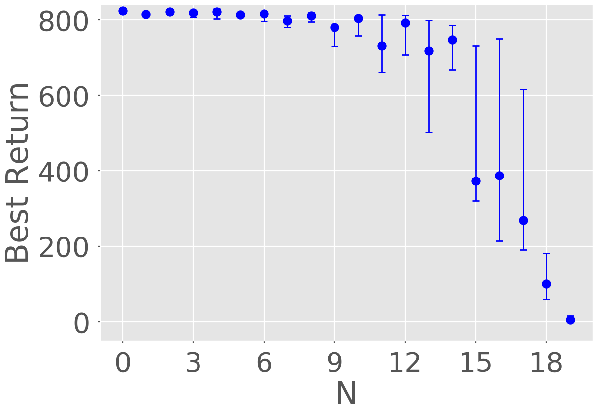
Refer to caption
(a) η1=0subscript𝜂10\eta_{1}=0
Refer to caption
(b) η1=0.1subscript𝜂10.1\eta_{1}=0.1
Refer to caption
(c) η1=0.2subscript𝜂10.2\eta_{1}=0.2
Refer to caption
(d) η1=0.3subscript𝜂10.3\eta_{1}=0.3
Refer to caption
(e) η1=0.4subscript𝜂10.4\eta_{1}=0.4
Refer to caption
(f) η1=0.5subscript𝜂10.5\eta_{1}=0.5
Refer to caption
(g) η1=0.6subscript𝜂10.6\eta_{1}=0.6
Refer to caption
(h) η1=0.7subscript𝜂10.7\eta_{1}=0.7
Refer to caption
(i) η1=0.8subscript𝜂10.8\eta_{1}=0.8
Refer to caption
(j) η1=0.9subscript𝜂10.9\eta_{1}=0.9
Refer to caption
(k) η1=1.0subscript𝜂11.0\eta_{1}=1.0
Figure 4: Ablation study for η1subscript𝜂1\eta_{1}.

6.9.3 Ablation study for η2subscript𝜂2\eta_{2}
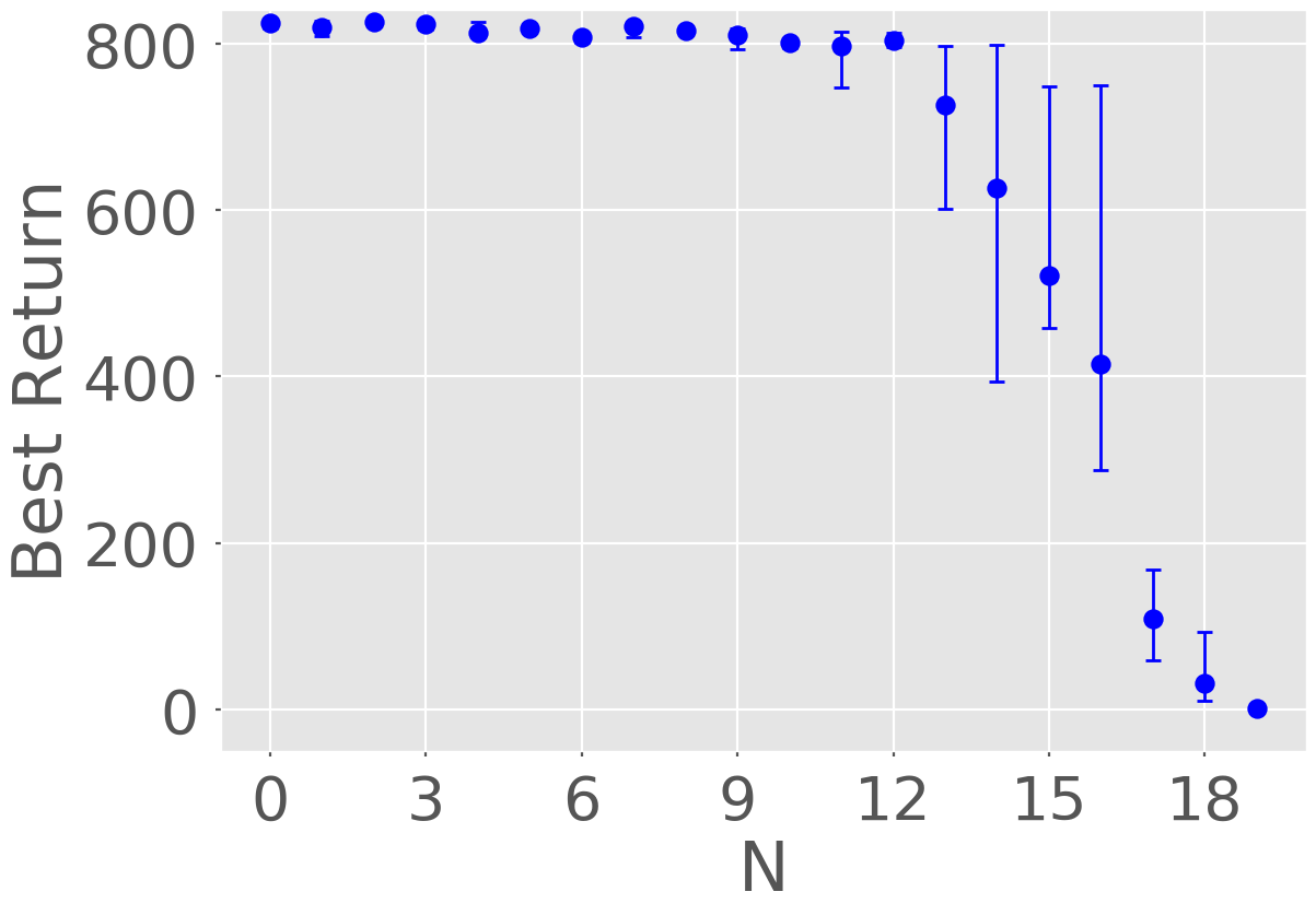
Refer to caption
(a) η2=0subscript𝜂20\eta_{2}=0
Refer to caption
(b) η2=0.1subscript𝜂20.1\eta_{2}=0.1
Refer to caption
(c) η2=0.2subscript𝜂20.2\eta_{2}=0.2
Refer to caption
(d) η2=0.3subscript𝜂20.3\eta_{2}=0.3
Refer to caption
(e) η2=0.4subscript𝜂20.4\eta_{2}=0.4
Refer to caption
(f) η2=0.5subscript𝜂20.5\eta_{2}=0.5
Refer to caption
(g) η2=0.6subscript𝜂20.6\eta_{2}=0.6
Refer to caption
(h) η2=0.7subscript𝜂20.7\eta_{2}=0.7
Refer to caption
(i) η2=0.8subscript𝜂20.8\eta_{2}=0.8
Refer to caption
(j) η2=0.9subscript𝜂20.9\eta_{2}=0.9
Refer to caption
(k) η2=1.0subscript𝜂21.0\eta_{2}=1.0
Figure 5: Ablation study for η2subscript𝜂2\eta_{2}.

We clarify that figure 5(k) shows no progress because the algorithm diverged for the chosen step-sizes in this ablation study.