Velocity distribution function of Na released by photons from planetary surfaces

Abstract

In most surface-bound exospheres Na has been observed at altitudes above what is possible by thermal release. Photon stimulated desorption of adsorbed Na on solid surfaces has been commonly used to explain observations at high altitudes. We investigate three model velocity distribution functions (VDF) that have been previously used in several studies to describe the desorption of atoms from a solid surface either by electron or by photon bombardment, namely: the Maxwell-Boltzmann (M-B) distribution, the empirical distribution proposed by [1] for PSD, and the Weibull distribution. We use all available measurements reported by [2, 3] to test these distributions and determine which one fits best (statistically) and we discuss their physical validity. Our results show that the measured VDF of released Na atoms are too narrow compared to Maxwell-Boltzmann fits with supra-temperatures as suggested by [3]. We found that a good fit with M-B is only achieved with a speed offset of the whole distribution to higher speeds and a lower temperature, with the offset and the fit temperature not showing any correlation with the surface temperature. From the three distributions we studied, we find that the Weibull distribution provides the best fits using the temperature of the surface, though an offset towards higher speeds is required. This work confirms that Electron-Stimulated Desorption (ESD) and Photon-Stimulated Desorption (PSD) should produce non-thermal velocity (or energy) distributions of the atoms released via these processes, which is expected from surface physics. We recommend to use the Weibull distribution with the shape parameter $\kappa$=1.7, the speed offset $v_{0}$ = 575 m/s, and the surface temperature to model PSD distributions at planetary bodies.

1 Introduction

Since the advent of space exploration and ground-based observations that made possible the detection of, for instance, the tenuous Na and K atmospheres of Mercury and the Moon, several studies and experiments have been carried out on lunar mineral grains and simulant materials (e.g. [4]). Some studies have focused on investigating the most relevant desorption processes for alkalis (e.g. [5, 6, 2, 3, 7]) to better understand the interaction between the surface and the exosphere of the planetary body under study.

Neutral sodium in the exospheres of the Moon and Mercury is one of the most studied alkali metals since it is relatively easy to observe from the Earth, but for several decades there has been controversy concerning the processes promoting it into the atmosphere. One of the few experimental results in the laboratory studying the sodium release processes happening on Mercury’s surface are the experiments by [2, 3]. These authors studied the desorption induced by electronic transitions (DIET) of Na adsorbed on model mineral surfaces and lunar basalt samples. In particular, they measured velocity distribution functions (VDF) of Na released via ESD from SiO₂ surfaces and found it to be “clearly non-thermal” with respect to the surface temperature, similar to that of a 1200 K Maxwellian but with a higher-energy tail. The VDF of ESD from a lunar basalt sample was found to have a smaller offset in speed compared to that of SiO₂, with a peak around 0.8 km/s instead of 1 km/s [3]. Since ESD is a charge transfer process leading to electronic excitations similar to PSD, with comparable cross sections and an identical excitation threshold of $\geq$4 to 5 eV [2], the VDF distributions of released sodium are quite similar, so that ESD measurements can be substituted for the effects of UV photons. Since then, people have interpreted these VDFs using either thermal (Maxwellian) or non-thermal distributions. In previous studies a Maxwell- Boltzmann velocity distribution has been assumed with temperatures in the range: $T_{s}=$ 1200–1500 K (e.g. [8, 9, 10, 11]).

In other studies, non-thermal high-energy tail distributions have been assumed, for instance the energy distribution function (EDF) used by [12] for ESD from icy surfaces, which was later used and modified by [1] to model PSD of volatiles to determine the Na and K density profiles in the exosphere of Mercury. This modified version was also used by [13] and [14] to determine the escape rates of PSD process in Mercury’s exosphere, and by [15] and [16] to model lunar Na exosphere. A summary of previous works using different EDFs and arriving at different temperatures of the released Na atoms by PSD or ESD is shown in Table 1.

Table 1: Summary of different EDFs or VDFs used.

Reference	Process	EDF/VDF	T (K)
[12]	ESD	$CEU^{\beta}/(E+U)^{2+\beta}$ (100 K ice surfaces)	600
[10]	PSD	M–B (fit to [2])	1500
[1]	PSD	adapted from [12]	1500
[8]	PSD	M–B (model lunar exosphere)	1200
[17]	PSD	Kappa (fit to [2])	800
[17]	PSD	M–B (fit to [3])	500

Hitherto we use the measurement results reported by [2, 3], more specifically, the reported VDFs for neutral Na from SiO₂ substrates and from lunar basalt samples. We examine the fitness of some distributions functions, namely the Maxwell-Boltzmann, the empirical energy distribution proposed by [1] for released volatiles from Mercury’s surface via PSD (named here after “E-PSD”) which is based on the one used by [12] for icy surfaces, and the Weibull distribution. Using the Graphical Residual Analysis (GRA), we determine which of the these distributions is statistically more adequate to explain the measurements and we discuss their physical validity.

The way the energy is imparted to a photodesorbed atom from Mercury’s surface (or similar planetary surfaces) is not through a thermal process, but rather by single electronic excitations. Choosing an appropriate model of the EDF/VDF of the atoms released is important to properly interpret Na measurements in planetary exospheres, which are often assumed to have temperatures way above the surface temperature (see review by [11] or the work by [18], for instance). This work aims to clarify the implications of assuming either thermal or non-thermal energy distributions of atoms released by PSD and ESD from planetary surfaces not protected by an atmosphere, like the majority of the planetary objects of the solar system.

In Section 2 we give a general physical description of ESD and PSD processes, and in Section 3 we describe the results from experiments by [2, 3]. The measurements reported from these experiments are used for the statistical analysis in Section 4, where we present the mathematical description of the different probability distribution functions used to fit these measurements. We briefly describe in Section 4.4 the GRA we used to test the model distribution described in the previous section. In Section 5 we show the results of the fitting and the GRA, we discuss the physical interpretations in Section 6, and we conclude in Section 7.

2 Desorption Induced by Electronic Transitions (DIET)

DIET phenomenon refers to both the electron-stimulated desorption (ESD) and the photon-stimulated desorption (PSD). Desorption of atoms on the surface occurs when the surface is bombarded by electrons or by photons with sufficient energy to induce transitions to repulsive electronic states of the atom. The released particles are supra-thermal because the absorbed UV photon has energies way in excess compared to thermal energies of the surface, which leads to the excitation of an anti-bonding state, see Fig. 2 for a schematic representation of the process.

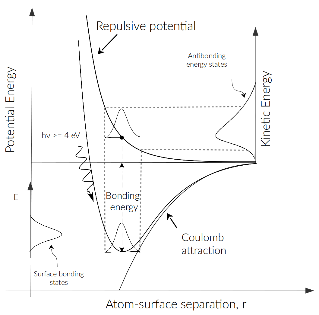
Figure 1: Schematics of the potential energy as function of the atom-surface separation, $r$, of the photon-stimulated desorption of surface species.

Figure 1 illustrates a typical DIET process where a bond of an atom on the surface is excited into an antibonding state induced by electron or photon absorption through a valence or core hole ionization process. [19] showed that valence excitations that include one-electron processes can lead to a long lasting (of the order of 10^-15 to 10^-14 s) antibonding repulsive state, from which desorption occurs. [19] also showed that “ESD and PSD of ions from both covalently bonded and ionically bonded surface species proceed through multielectron excitations that produce highly repulsive electronic states”; these states have sufficiently long lifetimes ($\sim 10^{-14}$ s) that electronic energy can be converted to atomic motion, i.e., kinetic energy.

Such electronic excitation events are by nature non-thermal, therefore it is expected that the speed EDF/VDF of the species in the anti-bonding state has to be non-thermal with a high-energy tail.

3 Experiments

[2, 3] studied the desorption induced by electronic transitions (DIET) of Na adsorbed on amorphous, stoichiometric SiO₂ films and on a lunar basalt sample. Experiments included ESD and PSD as release processes. Reported measurements were done with a different coverage and and different substrate temperature: $\sim 0.22$ ML of Na adsorbed at $\sim$250 K on SiO₂ films [2], and $\sim 0.5$ ML of Na adsorbed at 100 K on a lunar basalt sample [3]. Details of how the experiments were performed can be found in the respective references.

What is important to mention is that their results show that the ESD and PSD of Na from SiO₂ films and lunar basalt samples occur at threshold photon energies as low as h$\nu\sim$4 eV and that desorbing atoms have suprathermal velocities. Although they used ESD and PSD as release mechanisms, they only reported the VDF of Na released via ESD and later considered ESD results applicable to PSD as they are equivalent.

The VDFs were interpreted by [2] as the ability of photons with threshold energies $\geq$3–4 eV to induce electron transfer from an electronic state in the bulk, or from a surface state, to the unoccupied Na⁺ 3s level. When the 3s level is occupied, the Na⁰ atom has a larger radius compared to the original Na⁺ ion thus the atom is now in a highly repulsive configuration, from which desorption from the surface occurs.

The velocity distribution for desorbing Na⁰ from SiO₂ films at 250 K we use in this work can be seen in Figure 2.(a) in [2]. Later, [3] did similar experiments on a lunar basalt sample at 100 K and the reported VDF is shown in Figure 3 in their work. The peaks of the VDFs corresponding to the 250 K and 100 K substrate temperatures were reported as 1000 m/s and 800 m/s, respectively. The latter was interpreted by the same authors as being similar to a $\sim 900$ K Maxwellian distribution. This temperature is obtained only when assuming that the peak speed of the distribution is equal to the thermal speed. Similarly, a $\sim 1650$ K Maxwellian would be obtained for the VDF corresponding to the 250 K substrate, but in the literature people have used Maxwellian VDFs in the range of $1200$–$1500$ K.

4 Velocity distribution functions

To mathematically best describe the published laboratory measurements [2, 3] and planetary observations (e.g. [18]) we seek a VDF that has a characteristic energy significantly higher than what corresponds to the surface temperature and that tails towards higher speeds. The second goal of the seeked model distribution function is a parametrization that allows for its applications at other surface temperatures than the measured ones, in particular for surfaces of Mercury and the Moon.

In the following we will present three different VDFs, two of which have been used in the literature, namely the Maxwell-Boltzmann distribution and an ad-hoc distribution originally used for the icy surfaces of Jupiters moons [12]. The third distribution is a Weibull distribution, which has not been used so far to model the VDFs for ESD and PSD particle release.

Because no angular distribution is given in the experiments, we assume that the setup was in such a way that the field of view of the detector observing Na atoms that moved in just one direction. This leads us to consider only one-dimensional VDF. Furthermore, for our derivations of the VDFs we assume that the main influencing parameter is the surface temperature. The other two parameters that could influence the VDF is the Na coverage and the substrate material. Because of the limited data available we can not take these into consideration in this work. We discuss the implications of these assumptions in Section 6.

4.1 Maxwell-Boltzmann distribution function

The one-dimensional Maxwell-Boltzmann VDF, which reads in its normalised form as:

$$f(v-v_{0})=\left(\frac{m}{2\pi k_{B}T}\right)^{1/2}\phantom{x}\mathrm{exp}\left[-\displaystyle\frac{m}{2k_{B}T}(v-v_{0})^{2}\right]$$ (1)

where $k_{B}$ is the Boltzmann constant, $T$ is the gas temperature in Kelvin, $v_{0}$ is the speed offset in m/s.

If we assume that the most probable speed (peak of the distribution) is equal to the thermal speed of the particles released from the surface, we can derive the characteristic temperature from $T=m\bar{v}^{2}/(2k_{B})$, where $k_{B}$ is the Boltzmann constant. Therefore, a temperature of $T\sim 1400$ K is obtained if the peak of the distribution is at $\bar{v}\sim 1000$ m/s, which corresponds to the released Na peak speed measured from a 250 K substrate [2]. Similarly, a temperature of $T\sim 900$ K is obtained from the peak of the distribution at $\bar{v}\sim 800$ m/s, which is the case of the peak in speed measured by [3] from a lunar basalt sample at 100 K. Nevertheless, a Maxwellian with $T=1200$ K has been more commonly assumed for the former measurements, and it is the one we will use in this work.

Figure 2 shows the measured VDFs and the various fitted VDFs. The grey-diamonds symbols in all the plots of Figure 2 are the measured VDFs of the released Na: in the left column are measurements on a 250 K substrate and in the right column on a 100 K substrate. The dashed-black curves in Figures 2 (a) and (d) are the M-B fits, with a temperature of $1200$ K and $900$ K, and shifted to higher speed by an offset of 1000 m/s and 730 m/s, respectively.

We searched for a better fit, which is easily obtained if we use a smaller temperature of the M-B distribution, which is still higher than the surface temperature. Moreover, to obtain a good fit, these M-B distributions had to be shifted to higher speeds. These fits are presented as the solid-black curves in Figures 2 (a), with a $300$ K M-B, and (d), with a $150$ K M-B; and shifted in speed by an offset of 1000 m/s and 750 m/s, respectively.

From here on we will address the $150$ K and the $300$ K M-B distributions as “low” temperature M-B fits, and the $900$ K and the $1200$ K M-B distributions as the “high” temperature M-B fits.

4.2 Empirical PSD distribution function

We present here the empirical energy distribution function, EPSD, for PSD at Mercury and the Moon [20, 21, 1], $f(E)_{\rm PSD}$. It is based on the distribution given by [12], and which was adapted for Mercury’s surface by accounting for the extra energy in the desorption process and by including an energy cut-off. The normalised distribution is given as:

$$f(E)_{\rm PSD}=\beta(1+\beta)\frac{EU^{\beta}}{(E+U)^{2+\beta}}\left(1-\sqrt{\frac{E+U}{E_{max}}}\right)$$ (2)

where $U$ is the characteristic energy of particles released by PSD, $\beta$ is the shape parameter of the distribution, and $E_{max}=4$ eV is the maximum energy the released particles can have based on the available energy of the photons for the reported experiments. The characteristic energy, $U$, is related to the surface temperature by [20]:

$$U=\frac{k_{B}T_{0}}{e}\phantom{xx}\mathrm{in}\phantom{x}\mathrm{[eV]}\phantom{xx}\mathrm{with}\phantom{xx}T_{0}=T_{i}+T_{s},$$ (3)

where $e$ is the elementary charge, $T_{s}$ is the local surface temperature, and $T_{i}$ is the energy contribution by the desorption process, which is species specific; for sodium we used $T_{\mathrm{Na}}=600$ K. This is based on observations at Mercury [22].

To derive the VDF from the energy distribution stated above, we substitute $E$ for $\frac{mv^{2}}{2e}$ into Eq. 2 to have the appropriate units. First, the cut-off term is re-written as:

$$1-\sqrt{\frac{E+U}{E_{max}}}=1-\sqrt{\frac{\frac{m}{2e}v^{2}+Ue}{v_{max}}}$$

where $v_{max}=\sqrt{2eE_{max}/m}$. The new normalization constant is obtained after integrating in the range $v\in[0,\infty)$, as follows:

$$1=\bigintsss_{0}^{\infty}f(E)_{\rm PSD}dE=\bigintsss_{0}^{\infty}\frac{mv}{e}\cdot f(v)_{\rm PSD}dv$$ (4)

where we have used: $dE=\frac{mv}{e}dv$. Thus, we arrive at the VDF:

$$f(v)_{\rm PSD}=\beta(1+\beta)\frac{\displaystyle m^{2}/(2e^{2})}{\displaystyle(m/2e)^{2+\beta}}\phantom{x}\frac{v^{3}U^{\beta}}{(v^{2}+2eU/m)^{2+\beta}}\left(1-\sqrt{\frac{\frac{m}{2e}v^{2}+Ue}{v_{max}}}\right)$$ (5)

We perform two different fits using Eq. 5: the first is using the same parameters adapted for the release of Na atoms from the surface of Mercury proposed by [1], i.e., $\beta=0.7$ and $T_{0}=T_{i}+T_{s}$, where $T_{\mathrm{Na}}=600$ K and $T_{s}=[250,100]$ K. These fits are shown as the dashed-black curves in Fig. 2 (b) and (e) and correspond to the $T_{0}=850$ K and the $T_{0}=700$ K. Secondly, we use the same Eq. 5 but without an offset in temperature, same shape parameter, $\beta=0.7$, and an arbitrary offset towards higher speeds to obtain a better fit. These fits are shown as the solid-black curves, with an offset of $v_{0}\sim 500$ m/s for the distribution of the 250 K measurements and $v_{0}\sim 400$ m/s for the distribution of the 100 K measurements; both with the same shape parameter $\beta=0.3$.

4.3 Weibull distribution function

The Weibull distribution allows for a wide range of shapes using only two parameters for its definition. The normalised Weibull distribution for the random variable $v$ is defined as:

$$f(v;\lambda,\kappa)=\begin{cases}\frac{\kappa}{\lambda}\left(\frac{v}{\lambda}\right)^{\kappa-1}\displaystyle\mathrm{e}^{-(v/\lambda)^{\kappa}}&:v\geq 0,\\ 0&:v<0\end{cases}$$ (6)

where $\kappa$ is the dimensionless shape parameter and $\lambda>0$ is the scale parameter of the distribution (in m/s). The scale parameter $\lambda$ is obtained after calculating the mean (first central moment) of the probability distribution function:

$$\bar{v}=\bigintsss_{-\infty}^{\infty}vf(v,\lambda,\kappa)dv=\bigintsss_{0}^{\infty}v\frac{\kappa}{\lambda}\left(\frac{v}{\lambda}\right)^{\kappa-1}\mathrm{e}^{-(v/\lambda)^{\kappa}}dv=\lambda\Gamma\left(1+\frac{1}{\kappa}\right)$$

It follows that:

$$\lambda=\displaystyle\frac{\bar{v}}{\Gamma\left(1+\frac{1}{\kappa}\right)}.$$

The surface, which is the staring point of the desorbed atoms, has a given temperature $T_{s}$. This surface temperature will cause an energy broadening of the electronic transition induced by the adsorption of the UV photon (as depicted in Fig. 1). Therefore, the related kinetic energy of the desorbed Na of $\displaystyle\frac{1}{2}m\bar{v}^{2}=\frac{3}{2}k_{B}T_{s}$ folds into the distribution. Since we consider the one-dimensional case, we have $\bar{v}=\displaystyle\sqrt{\frac{3k_{B}T_{s}}{m}}$. Substituting $\bar{v}$ in the expression for $\lambda$:

$$\lambda=\displaystyle\frac{\sqrt{\frac{3k_{B}T}{m}}}{\Gamma\left(1+\frac{1}{\kappa}\right)}$$ (7)

thus, the normalised Weibull distribution for $v\geq 0$ is:

$$f(v,v_{0},\kappa)= \kappa\phantom{.}\Gamma\left(1+\frac{1}{\kappa}\right)\left(\frac{m}{3k_{B}T_{s}}\right)^{1/2}\left[(v-v_{0})\phantom{.}\sqrt{\frac{m}{3k_{B}T_{s}}}\Gamma\left(1+\frac{1}{\kappa}\right)\right]^{\kappa-1}\times$$

$$\times\mathrm{exp}\left[-\left((v-v_{0})\phantom{.}\sqrt{\frac{m}{3k_{B}T_{s}}}\Gamma\left(1+\frac{1}{\kappa}\right)\right)^{\kappa}\right]$$ (8)

where $v_{0}$ is the offset speed, and $\kappa$ is the shape parameter, which is an implicit function that is usually determined by numerical means (see [23]).

The Weibull fits are represented as the solid-black curves shown in Figures 2 (c) and (f). For both measured VDFs we looked for a good fit with the same shape parameter, $\kappa$. We get reasonably good fits for both data sets with a single set of parameters using $\kappa=1.7$ and $v_{0}=575$ m/s, and using actual the surface temperature $T_{s}$ to derive $\lambda$ from Eq. 7. We suggest to use this set of parameters ($\kappa,v_{0}$) for modelling the PSD processes for planetary surfaces, since only the surface temperature is needed as input parameter for the distribution function.

Of course, better fits to the two data sets can be achieved with the Weibull distribution function allowing for different parameters for the different fits. For the VDF from the substrate at 250 K the Weibull distribution with $T_{s}$ = 250 K and $\kappa=1.8$ with an offset of $v_{0}=600$ m/s makes the best fit, whereas the Weibull distribution with $T_{s}$ = 100 K, $\kappa=1.8$ and an offset of $v_{0}=500$ m/s fits best the VDF from the 100 K substrate. Unfortunately, these derived parameters do not allow any meaningful extension for other surface temperatures.

4.4 Graphical Residual Analysis (GRA)

The measurements and the fit functions as shown in the panels of Figures 2 from (a)–(f) are useful for showing the relationship between the data and the proposed models; however, it can hide crucial details about the fit function. Plotting the residuals can help show these details well, and should be used to check the quality of the fit. The Graphical Analysis of the Residuals (GRA) is a common and powerful technique to determine if the model needs refinement or to verify if the underlying assumptions of the model are met. The normal probability plot is a useful residual plot of this model, which we also include in our analysis. In this section we briefly describe the GRA method.

The GRA entails a basic, though not quantitatively precise, evaluation of the differences between the observed values of the dependent variable after fitting a model to the data (residuals). The GRA is a visual examination of the residuals to look for obvious deviations from randomness.

Let us denote $y_{i}$ the measured value (i.e., the probability of a Na atom having a speed $v_{i}$) and $f(v_{i})$ the value from the model distribution. Thus, for every $v_{i}$, the residual of the $i^{th}$ observation is simply defined as the distance between the measured value and the theoretical value:

$$r_{i}=y_{i}-f(v_{i})\phantom{xx}i=1,2,\ldots,n.$$ (9)

where $n$ is the number of data points.

The corresponding residuals plots for the different fits are shown in the bottom left of each panel (a)–(f) in Figure 2. An overly simplified but straightforward way to assess the adequacy of the fit is by looking at the general tendency of the residuals plot along with the absolute value of the sum of residuals (shown in Table 2). If the overall residual values are close to zero, then the absolute value of their sum would also be close to zero, which can be a direct evidence that the model is a good fit to the observations. Conversely, if the residual values tend to be far away from zero, either below or above zero, then the absolute value of the sum will not be close to zero. However, if the residuals alternate evenly above and below zero, independently of the distance to zero, then the absolute value of the sum of the residuals will still be close to zero. Thus we have not enough information to conclude whether the model fits the observations.

One way to obtain more information about any tendencies in the residuals, for instance: suspected outliers, skewness to right or left, light-tailedness or heavy-tailedness, or mixtures of normal distributions is through the normal probability plot ([24]) because is a graphical technique for assessing whether or not the residuals are approximately normally distributed. If the residuals were perfectly normally distributed this would indicate that residuals have a random variation and then it would be reasonable to conclude that the model is adequate and differences are statistical. In other words, residuals that are perfectly normally distributed can be considered as noise.

The residuals are plotted against a theoretical normal distribution in such a way that the points should form an approximate straight line. The normal probability plot matches the quantiles of the residuals to the quantiles of a normal distribution. These plots are shown as the solid-grey lines at the bottom right corner of each panel (a)–(f) in Figure 2. Departures from this straight line indicate departures from normality. In the next section we show and interpret the results obtained. We followed the theory of GRA from [25] and also to interpret the results.

5 Results

In Section 4 we provided the mathematical description of three different model distributions and then searched for the best parameter combination to fit the measured VDFs under consideration. The different fits obtained are presented in this section in the main plots in Figure 2. How well the model distributions used so far fit the measurements is qualitatively estimated by virtue of the GRA. The results of the GRA are shown in the bottom part of each panel in Figure 2; the plots of residuals are shown in the bottom left and the normal probability plots are shown in the bottom right.

It is evident from the general features of the Maxwell-Boltzmann fits that the “high” temperature distributions shown in Figure 2 (a) and (d) are much too wide compared to the measured VDFs. In contrast, the two “low” temperature M-B distributions fit the bulk of the distributions significantly better, though underestimating the tails, and with the need for large speed offsets.

It is also clear that the E-PSD fits with the parameters adapted for the release of Na from the surface of Mercury are too wide and shifted compared to the measured distributions. Slightly better fits with the E-PSD function are obtained when $T_{0}=T_{s}$ is used and a speed offset is considered. However, these “low temperature” fits exhibit very long tails thus overestimating the observed values at higher speeds. Although there is no need to adjust an offset temperature, an arbitrary offset towards higher speeds is required to fit reasonably well the bulk of the measured distributions.

A more careful evaluation of the fits is done with the residuals plots together with the normal probability plots. The residuals are plotted against the speed and both axes have units of m/s. A reference line at $y=0$ is shown in grey scale to identify a change of sign toward positive or negative values.

The residuals of the two “high” temperature M-B are mostly negative except close to the peak of both distributions where they are almost zero. This is because this model function is far above the measured data and too wide compared to the measured distribution, which makes the residuals mainly have negative values. In fact, the absolute values of the total sum of the residuals of these fits are one order of magnitude larger than then rest of the fits, as can be seen in Table 2. The normal probability plot of the $1200$ K M-B distribution shows a strong linear dependence with the theoretical normal distribution between the first and the third quartile but it is not centered at zero and in the left and right ends the plot bends away from the hypothetical straight line. The normal probability plot of the 900 K M-B does not show any linear dependence with the theoretical normal distribution and it is not symmetrical around zero.

The residuals of the “low” temperature M-B fits seem more evenly distributed around zero, which makes the absolute value of the total sum of residuals close to zero. The normal probability plot of the $300$ K M-B fit exhibits oscillations around the straight line between the first and the third quartile and it bends above the straight line at the right and left ends. The normal probability plot of the 150 K M-B fit has a similar shape compared to the one at 900 K, but the plot is well centered around zero.

The residuals of the 850 K and the 700 K E-PSD fits are mostly negative but vary with a similar amplitude compared to the residuals of the 250 K and the 100 K E-PSD fits, which is expected from the shift in speed that the latter exhibits with respect to the measured distribution. The normal probability plots of the four cases with the E-PSD display a big deviation at the far ends and a moderately linear relationship with the theoretical values from the standard normal distribution between the first and the third quantile. This is a consequence of the heavy-tailed feature of the E-PSD distribution.

The large bend below the straight line displayed in the normal probability plot for the Weibull distribution with at temperature of 250 K reveals that the data are skewed to the left in comparison with the model distribution. This difference is more evident in the main plot between $\sim$450 m/s and $\sim$700 m/s, where the Weibull distribution underestimates the observations.

A common aspect of all the normal probability plots obtained is that they all exhibit deviations from the normal distribution, specially on either end of the speed range. In this case, the parent distribution from which the data were sampled is considered to be heavy-tailed because the right upper end of the normal probability plot bends over the hypothetical straight line that passes through the main body of the X-Y values of the normal probability plot, and when the left lower end bends below it ([25]).

It is clear from the normal probability plots presented here that none of the residuals of the proposed model distributions are normally distributed, i.e., that an optimal fit to the data has not been achieved. Nevertheless, it is undeniable that the deviations from normality and the absolute value of the sum of residuals of the “high” temperature M-B are much larger than those from the other model distributions. In comparison, the residual are smallest for the adapted E-PSD distributions, and Weibull second smallest for the 250 K substrate.

Table 2: Sum of residuals.

Substrate temperature: 250 K	Modeled temperature (K)	$\left|\displaystyle\sum_{i=0}^{n}r_{i}\right|$
Maxwell-Boltzmann 1D (“low” temperature)	300	49.44
Maxwell-Boltzmann 1D (“high” temperature)	1200	216.63
Empirical-PSD	250	71.80
Empirical-PSD	850	234.18
Weibull	250	50.49
Substrate temperature: 100 K
Maxwell-Boltzmann 1D (“low” temperature)	150	48.45
Maxwell-Boltzmann 1D (“high” temperature)	900	505.04
Empirical-PSD	100	60.61
Empirical-PSD	700	513.74
Weibull	100	74.71

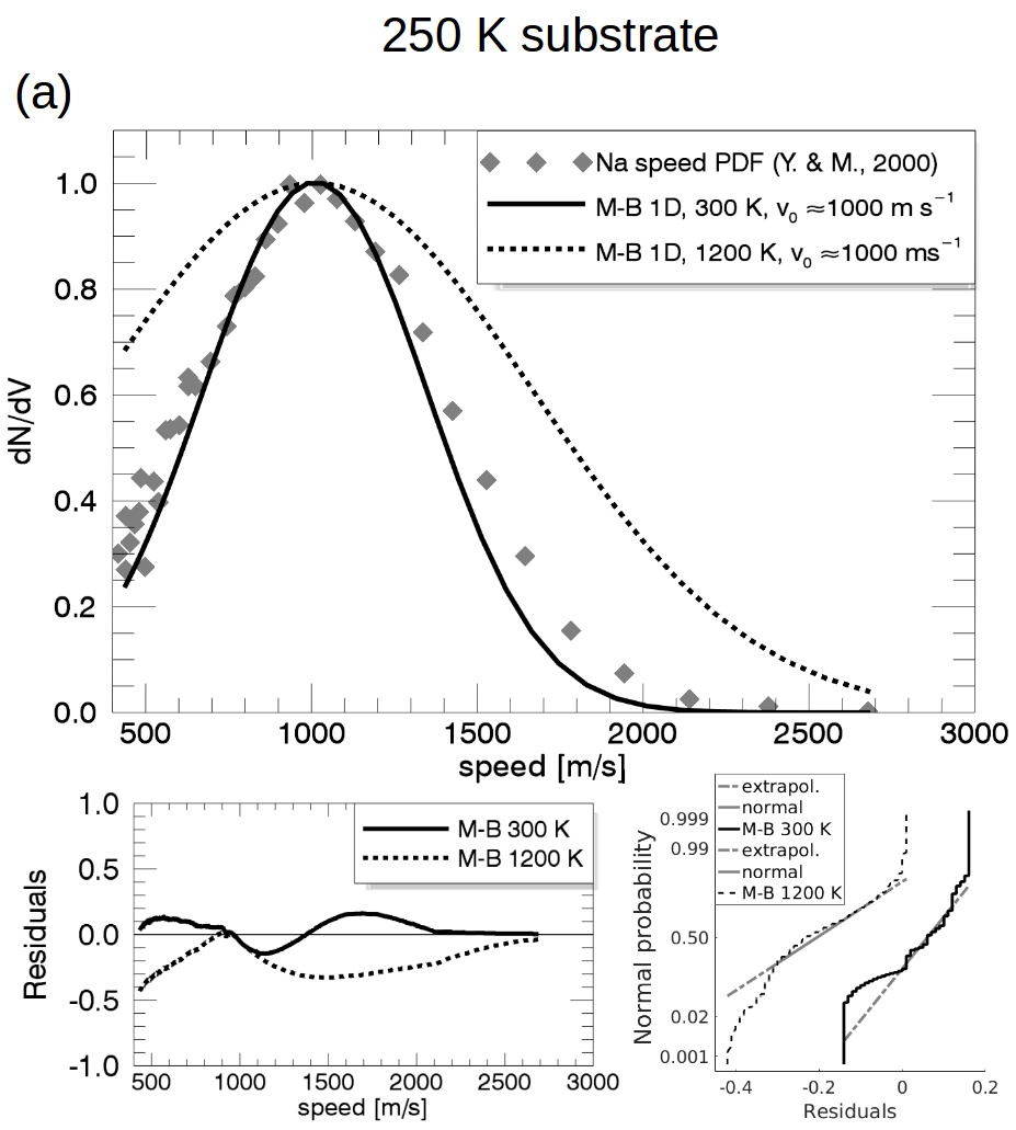
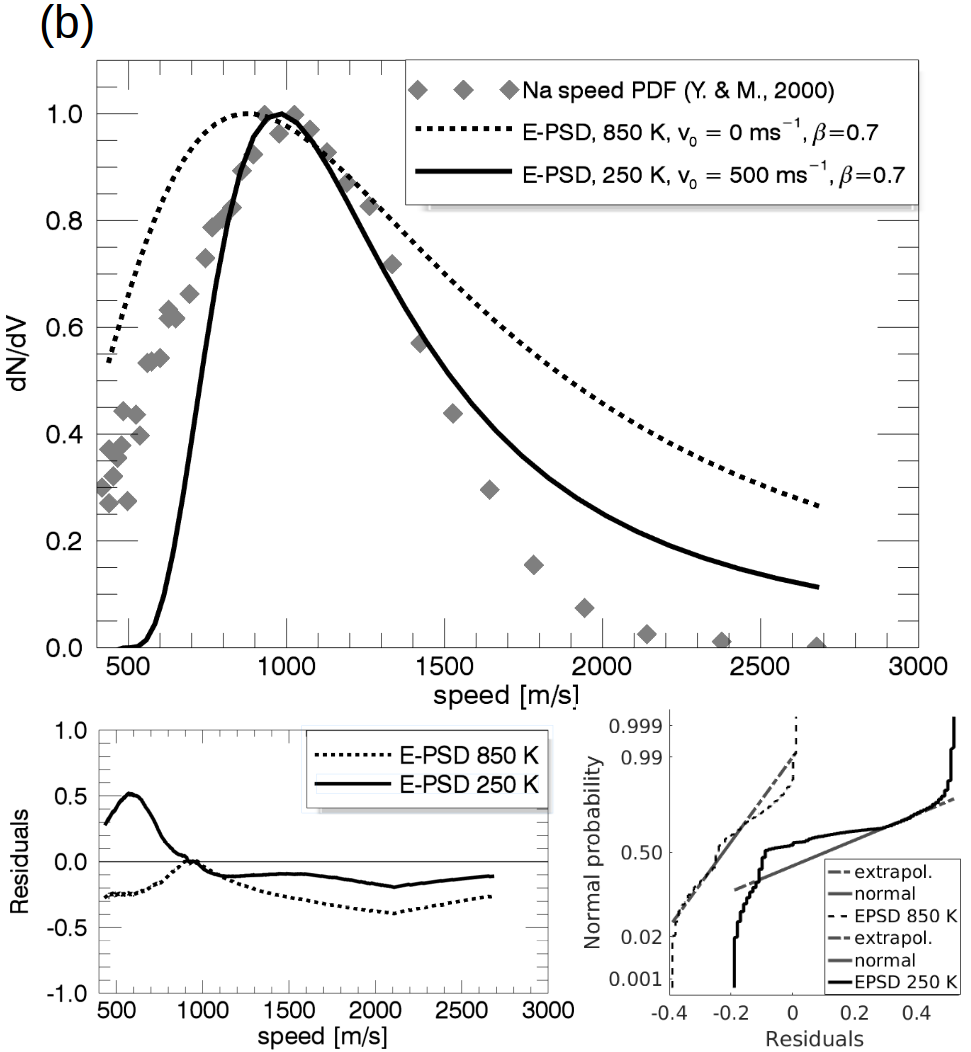
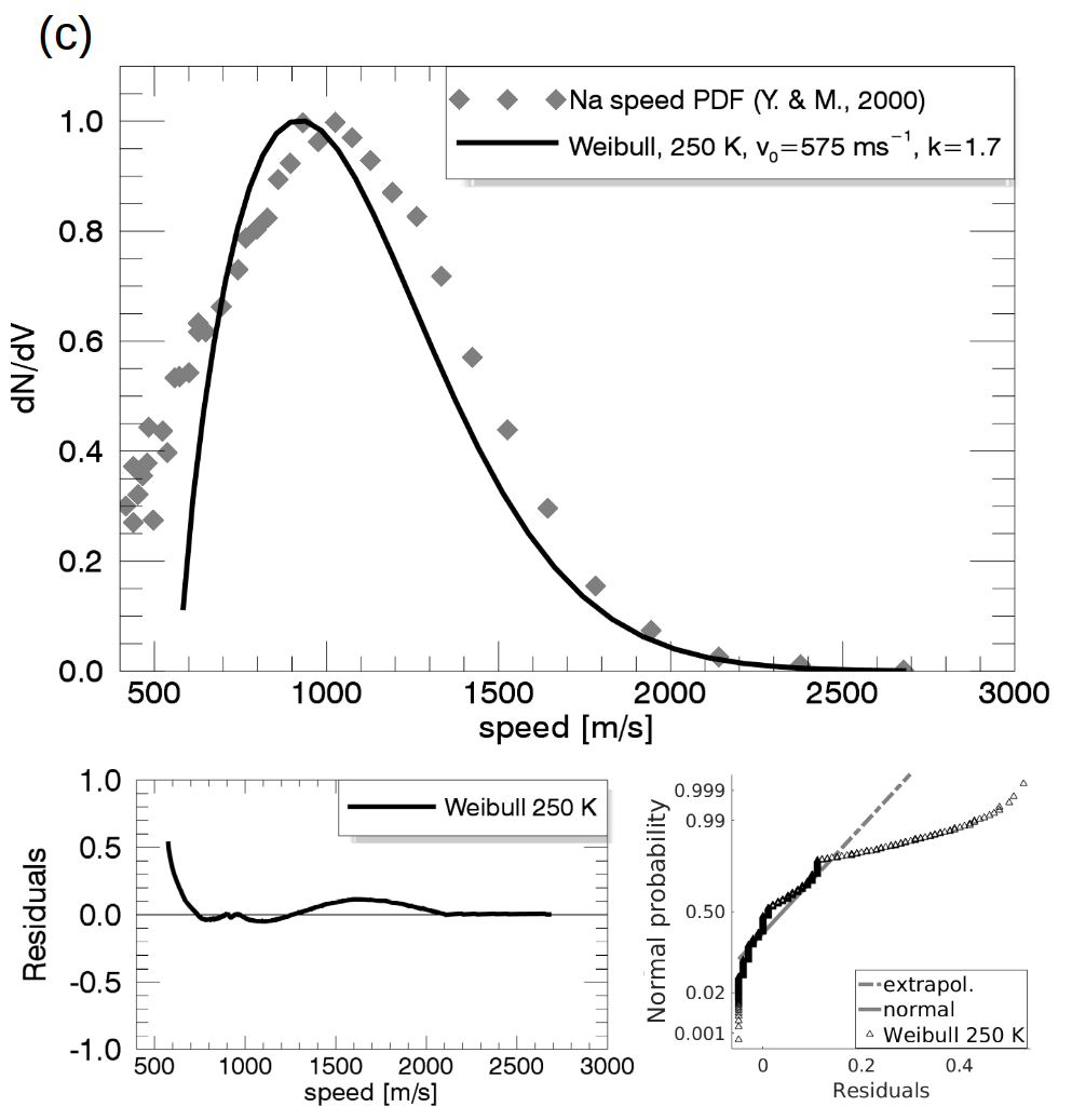
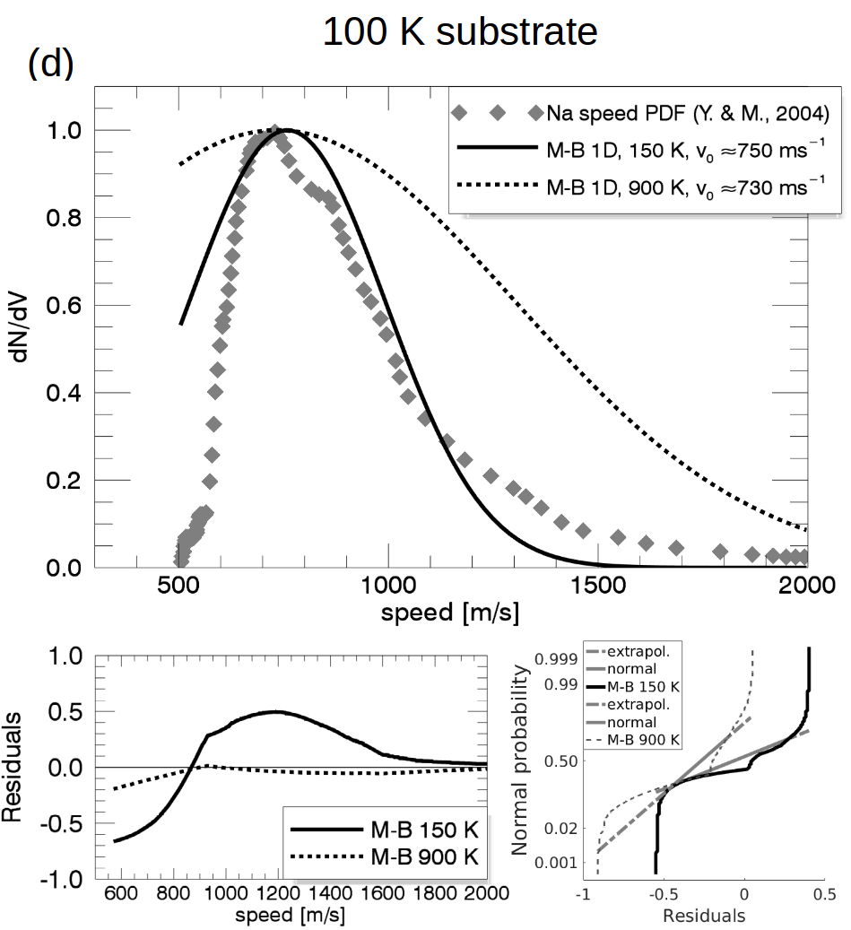
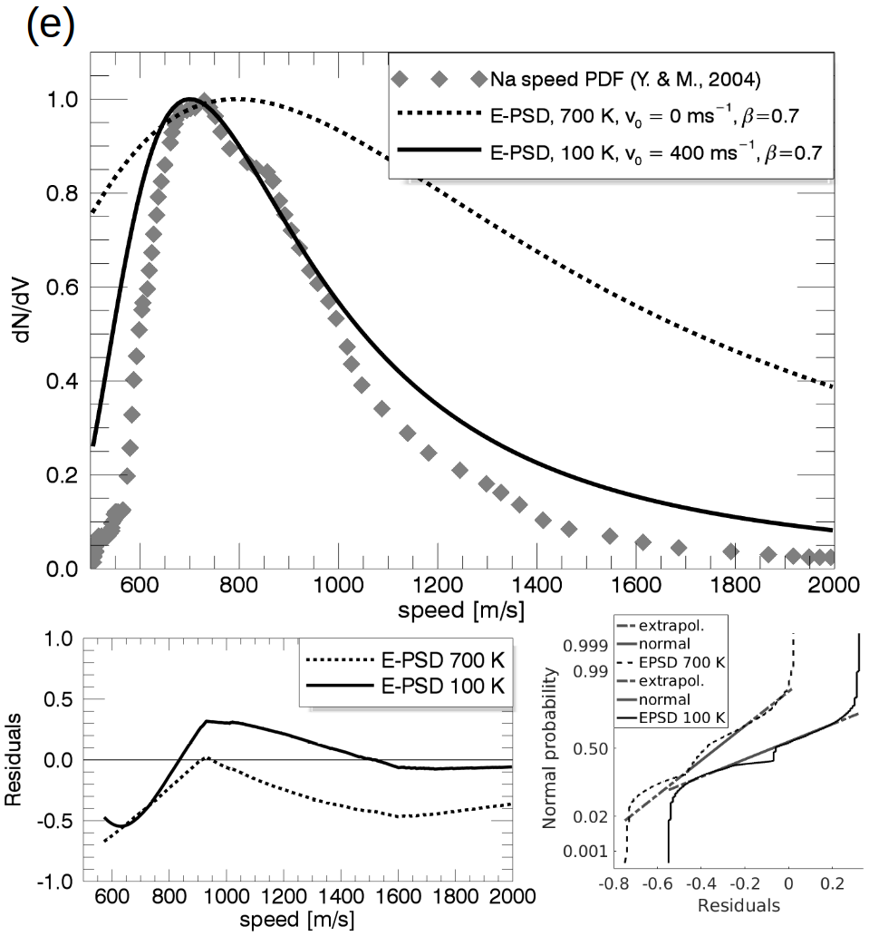
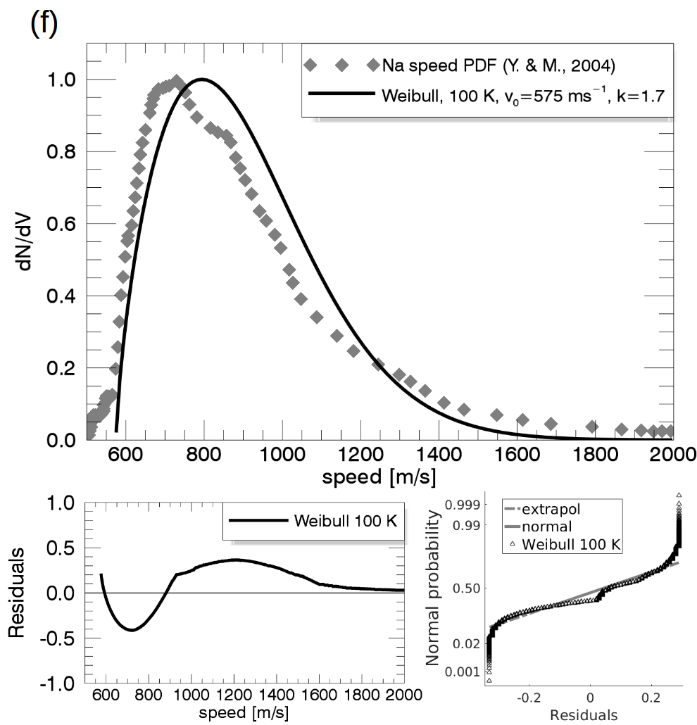
Figure 2: Main panels from (a) to (c): grey-diamonds are the VDFs from neutral Na on a 250 K lunar substrate (see [2]); same from (d) to (f) but experiments were performed on a lunar sample with a temperature of 100 K (see [3]). The “low” temperature M-B fits are shown as the solid-black curves and the “high” temperature M-B as the dashed-black curves. The dashed-black and the solid-black curves in (b) and (e) correspond to the Empirical-PSD distribution proposed by [1]. The solid-black curves in (c) and (f) are the Weibull fits. The residuals plots and the normal probability plots are shown in the bottom part of the main panels.

6 Discussion

In this work we test the statistical adequacy of three model distributions: the Maxwell-Boltzmann and two non-Maxwellian by means of the Graphical Residual Analysis. In this section we discuss which one we consider is physically more valid.

Concerning the results for the M-B fits: we find that the measured VDFs of released Na atoms are too narrow compared to the M-B fits suggested by [3] and as noted by other authors before. A considerably better fit with M-B is only achieved with an offset of the whole distribution to higher speeds and with a lower temperature. In all cases of fitting M-B distribution there is no correlation of the fit temperature and offset speed with the substrate temperature found.

Moreover, the applicability of the M-B distribution is limited to gases in thermodynamic equilibrium where the energy transfer is facilitated by particle collisions, and temperature is interpreted as the mean kinetic energy transferred from particle to particle when equilibrium is reached after sufficient collisions. These conditions certainly do not apply to the release of atoms by PSD, neither on Mercury surface (gas pressure at the surface $p<5\times 10^{-12}$ mbar) nor in the experiments done by [2, 3] where the residual gas is in a non-collisional regime (base pressure of $p<10^{-10}$ mbar). In PSD (and ESD) the energy transfer is carried by single electronic transitions on the surface of the substrate. Additionally, the 1D M-B distribution has a symmetric shape around the peak but the measured distributions do not exhibit this symmetry. The GRA results confirm this, particularly the two “high” temperature M-B are found to be statistically not appropriate. This is why the need of a non-thermal long-tailed VDF to explain the observed speeds is crucial.

With respect to the results obtained for the non-thermal distributions, it is evident that the E-PSD distribution adapted for Na released from the Mercury’s surface does not provide a good fit to the data, unless we consider a different temperature, and we include a rather arbitrary speed offset. This increases the amount of free parameters, which is unwanted, because it prevents generalisation and extrapolation to other surfaces temperatures.

On the other hand, even though we have no more data to constrain the parameters, the Weibull distribution represents the best of the three candidates. In terms of the shape, we found that if we use a value of $\kappa=1.7$, we obtain the best fit compared to the other distributions, specially the tail of the distribution. In terms of statistical adequacy, the GRA results show that the residuals are reasonably normally distributed and centered around zero, which is of advantage. The Weibull distribution is chosen to fulfill two requirements resulting from the observations: first observation is that the mean energy of the distribution is significantly above the thermal energy of the surface (given by experimental results and observations at Mercury and Moon); second observation is that the VDF tails towards higher energies (only from experimental results). The Weibull distribution satisfies these two conditions with a minimum number of free parameters: the characteristic energy parameter, $\lambda$, and the shape parameter, $\kappa$, as discussed above. Nevertheless, we admit that there is no rigorous physics argument for the use of the Weibull distribution.

With regard to the fitted offset of the distribution to higher speeds required for all the fits we do not have a rigorous explanation. Likely, the excess of energy the photon provides after the electronic excitation event, i.e., the fraction of the energy is spent in overcoming the Na binding energy during the photon-desorption and the remaining fraction is increasing the kinetic energy of the released atoms. This offset cannot be explained in terms of a bulk speed of the gas, as commonly assumed in the Kinetic Theory of Gases or Plasma Physics, where the bulk motion of the gas or plasma produces the offset and the temperature is explained by the microscopic motion through collisions. This does not apply to the experiments analyzed here since there is no collective behaviour.

Furthermore, and as mentioned in Section 4, we do not consider as fundamental parameters the Na coverage and the substrate material in our VDF derivations. With respect to how the Na coverage affects the VDF, [3] found that the ESD/PSD yields scale linearly with Na coverages $<1$ ML but the desorption yield curves are similar [2]. Because of this, we assume that there is no substantial difference between a Na coverage of 0.22 ML and 0.5 ML, therefore the VDF does not change dramatically either. However, in a similar experiment but different substrate material, [5] found that the ESD peak of the energy distributions for Na atoms extend toward low kinetic energies as the Na coverage increases above 0.125. Particularly, they found that the low-energy tail increases with increasing sodium coverage. In contrast, the results from other similar experiments by [7, 6], where they study desorption of Potassium, which show that when the substrate temperature is kept constant but the K coverage is decreased, this leads to a broadening of the VDF and shift of the peak towards higher energies, but no low-energy tail is observed when the coverage is increased. In any case, it is worth noting that the Na coverage used by [2, 3] are just experimental; the real coverage of Mercury’s or the Moon’s surface is likely much lower.

On the other hand, we consider the surface composition of minor importance because in [2, 3] experiments the Na was applied onto the surface by an external dispenser, thus the surface mostly served as a substrate.

Nonetheless, we recognize that the two last assumptions are a simplification, particularly given the fact that the lunar sample is a more complex oxide compare to the SiO₂ films. Unfortunately, there is not enough laboratory data to understand the effect of the surface material on the VDF. In this sense, the experiments done by [2, 3] are merely the starting point for models.

Similar attempts to describe the VDFs reported by [2, 3] with lower temperatures are, for instance, [17] who used a Kappa distribution with shape parameter $\kappa$= 1.8, with a temperature of 500 K, and with a offset of 0.5 km s^-1 to match the VDF of Na desorbed from a 100 K lunar sample. Whereas they fit a 800 K Maxwellian with an offset of 0.2 km s^-1, providing a good fit to the VDF of Na desorbed from a 250 K SiO₂ substrate.

7 Conclusions

Motivated by an ongoing debate whether or not ESD and PSD produce non-thermal EDF/VDF of the desorbed atoms in planetary exospheres, we compare the often-used model distributions previously proposed to fit the available observations. We use all the available measurements reported by [2, 3], who studied the ESD and PSD of Na adsorbed on SiO₂ films and lunar basalt samples. They reported suprathermal Na atoms with peak speeds of $\sim 800$ and $\sim 1000$ m s^-1, which were interpreted to come from a 900 K and a 1200–1500 K Maxwell-Boltzmann distribution, respectively.

Despite that only qualitative support for the non-thermal VDF of the released atoms via PSD is available (see Fig. 2), this study helps to confirm that: (1) the Maxwell-Boltzmann distribution is neither statistically nor physically adequate to describe non-thermal processes such as ESD and PSD; (2) ESD and PSD, being by nature produced by single electronic excitation events, produce non-thermal VDFs of the atoms released via these processes; and (3) an apparent “high” temperature is not needed when a non-thermal distribution, such as the Weibull distribution, is considered with the appropriate parameters. We recommend to use the Weibull distribution with $\kappa$=1.7, $v_{0}$ = 575 m/s, and the surface temperature to model PSD distributions at planetary bodies.

From observations we know that the large majority of planetary objects of the solar system have a surface bounded exosphere and are expected to have an extended Na exosphere. It is crucial to choose an appropriate model for the Na atoms release from the surface to properly interpret the measurements in planetary exospheres. This work is intended to resolve the implications of assuming different models of atoms released by PSD and ESD from any planetary surfaces not protected by an atmosphere.

References

References

- [1] P. Wurz, J. Whitby, U. Rohner, J. Martín-Fernández, H. Lammer, C. Kolb, Self-consistent modelling of mercury’s exosphere by sputtering, micro-meteorite impact and photon-stimulated desorption, Planet and Space Science 58 (2010) 1599–1616. doi:10.1016/j.pss.2010.08.003.
- [2] B. Yakshinskiy, T. Madey, Desorption induced by electronic transitions of na from sio2: relevance to tenuous planetary atmospheres, Surface Science 451, Issue 1 (2000) 160–165. doi:10.1016/S0039-6028(00)00022-4.
- [3] B. Yakshinskiy, T. Madey, Photon-stimulated desorption of na from a lunar sample: temperature-dependent effects, Icarus 168, Issue 1 (2004) 53–59. doi:10.1016/j.icarus.2003.12.007.
-
[4]
L. Keller, D. McKay, Discovery of
vapor deposits in the lunar regolith, Science 261 (5126) (1993) 1305–1307.
URL http://www.jstor.org/stable/2882155 -
[5]
V. Ageev, Y. A. Kuznetsov, T. E. Madey,
Electron-stimulated
desorption of sodium atoms from an oxidized molybdenum surface, Phys. Rev. B
58 (1998) 2248.
URL https://doi.org/10.1103/PhysRevB.58.2248 - [6] M. Wilde, I. Beauport, F. Stuhl, K. Al-Shamery, H.-J. Freund, Adsorption of potassium on at ionic and metallic coverages and uv-laser-induced desorption, Phys. Rev. B 59 (1999) 13401. doi:10.1103/PhysRevB.59.13401.
-
[7]
T. E. Madey, B. V. Yakshinskiy, V. N. Ageev, R. E. Johnson,
Desorption of alkali atoms and
ions from oxide surfaces: Relevance to origins of na and k in atmospheres of
mercury and the moon, Journal of Geophysical Research: Planets 103 (E3)
(1998) 5873–5887.
doi:10.1029/98JE00230.
URL http://dx.doi.org/10.1029/98JE00230 - [8] M. Sarantos, R. E. Hartle, R. M. Killen, Y. Saito, J. A. Slavin, A. Glocer, Flux estimates of ions from the lunar exosphere, Geophys. Res. Lett. 234 (4774) (1968) 316–322. doi:10.1029/2012GL052001.
-
[9]
R. Killen, D. Shemansky, N. Mouawad,
Expected emission from
mercury’s exospheric species, and their ultraviolet-visible signatures,
Astrophysical Journal Supplement 181 (2) (2009) 351–359.
URL http://stacks.iop.org/0067-0049/181/i=2/a=351 - [10] F. Leblanc, D. Delcourt, R. Johnson, Mercury’s sodium exosphere: magnetospheric ion recycling, J. Geophys. Res. 108 (2003) 5136–xxxx. doi:10.1029/2003JE002151.
- [11] R. M. Killen, G. Cremonese, H. Lammer, S. Orsini, A. E. Potter, A. L. Sprague, P. Wurz, M. L. Khodachenko, H. I. M. Lichtenegger, A. Milillo, M. A., Processes that promote and deplete de exosphere of mercury, Space Science Review 132 (2007) 433–509. doi:10.1007/s11214-007-9232-0.
- [12] R. Johnson, F. Leblanc, B. Yakshinskiy, T. Madey, Energy distributions for desorption of sodium and potassium from ice: the na/k ratio at europa, Icarus 156 (2002) 136–142. doi:10.1006/icar.2001.6763.
- [13] C. A. Schmidt, J. Baumgardner, M. Mendillo, J. K. Wilson., Escape rates and variability constraints for high-energy sodium sources at mercury, J. Geophys. Res. 117. doi:10.1029/2011JA017217.
- [14] A. Mura, P. Wurz, H. I. M. Lichtenegger, H. Schleicher, H. Lammer, D. Delcourt, A. Milillo, S. Orsini, S. Massetti, M. L. Khodachenko, The sodium exosphere of mercury: Comparison between observations during mercury’s transit and model results, Icarus 200 (1) (2009) 1–11. doi:doi:10.1016/j.icarus.2008.11.014.
- [15] V. Tenishev, M. Rubin, O. Tucker, M. Combi, M. Sarantos, Kinetic modeling of sodium in the lunar exosphere, Icarus 226 (2) (2013) 1538–1549. doi:10.1016/j.icarus.2013.08.021.
- [16] A. Sprague, M. Sarantos, D. Hunten, R. Hill, R. Kozlowski, The lunar sodium atmosphere: April–may 1998, Canadian Journal of Physics 118 (2012) 4564–4571. doi:doi:10.1139/p2012-072.
- [17] C. A. Schmidt, Monte carlo modeling of north-south asymmetries in mercury’s sodium exosphere, J. Geophys. Res. Space Physics 118 (2013) 4564–4571. doi:10.1002/jgra.50396.
- [18] T. Cassidy, A. W. Merkel, M. H. Burger, M. Sarantos, R. M. Killen, W. E. McClintock, V. J. R. J., Mercury’s seasonal sodium exosphere: Messenger orbital observations, Icarus 248 (2015) 547–559. doi:10.1016/j.icarus.2014.10.037.
- [19] T. E. Madey, Electron- and photon-stimulated desorption: Probes of structure and bonding at surfaces, Science, New Series 234 (4774) (1968) 316–322. doi:10.1126/science.234.4774.316.
- [20] P. Wurz, H. Lammer, Monte-carlo simulation of mercury’s exosphere, Icarus 164 (1) (2003) 1–13. doi:10.1016/S0019-1035(03)00123-4.
- [21] P. Wurz, U. Rohner, J. Whitby, C. Kolb, H. Lammer, P. Dobnikar, J. Martín-Fernández, The lunar exosphere: The sputtering contribution, Icarus 191 (2007) 486–496. doi:10.1016/j.icarus.2007.04.034.
- [22] R. Killen, A. Potter, A. Fitzsimmons, T. Morgan, Sodium d2 line profiles: clues to the temperature structure of mercury’s exosphere, Planet. Space Sci. 47 (1999) 1449–1458. doi:10.1016/S0032-0633(99)00071-9.
-
[23]
P. Bhattacharya,
A study
on weibull distribution for estimating the parameters, Journal of Applied
Quantitative Methods 5 (2) (2010) 234–241.
URL http://jaqm.ro/issues/volume-5,issue-2/pdfs/bhattacharya.pdf - [24] J. M. Chambers, W. S. Cleveland, B. Kleiner, P. A. Tukey, Graphical methods for data analysis, Wadsworth International Group, Belmont, CA.
- [25] StatGuide, https://www.quality-control-plan.com/StatGuide/sghome.html, [Online; accessed 19-November-2017] (1996).