Two-sample tests for relevant differences in the
eigenfunctions of covariance operators

Abstract

This paper deals with two-sample tests for functional time series data, which have become widely available in conjunction with the advent of modern complex observation systems. Here, particular interest is in evaluating whether two sets of functional time series observations share the shape of their primary modes of variation as encoded by the eigenfunctions of the respective covariance operators. To this end, a novel testing approach is introduced that connects with, and extends, existing literature in two main ways. First, tests are set up in the relevant testing framework, where interest is not in testing an exact null hypothesis but rather in detecting deviations deemed sufficiently relevant, with relevance determined by the practitioner and perhaps guided by domain experts. Second, the proposed test statistics rely on a self-normalization principle that helps to avoid the notoriously difficult task of estimating the long-run covariance structure of the underlying functional time series. The main theoretical result of this paper is the derivation of the large-sample behavior of the proposed test statistics. Empirical evidence, indicating that the proposed procedures work well in finite samples and compare favorably with competing methods, is provided through a simulation study, and an application to annual temperature data.

Keywords: Functional data; Functional time series; Relevant tests; Self-normalization; Two-sample tests.

1 Introduction

This paper develops testing tools for two independent sets of functional observations, explicitly allowing for temporal dependence within each set. Functional data analysis has become a mainstay for dealing with those complex data sets that may conceptually be viewed as being comprised of curves. Monographs detailing many of the available statistical procedures for functional data are Ramsay and Silverman, (2005) and Horváth and Kokoszka, (2012). This type of data naturally arises in various contexts such as environmental data (Aue et al.,, 2015), molecular biophysics (Tavakoli and Panaretos,, 2016), climate science (Zhang et al.,, 2011; Aue et al., 2018a, ), and economics (Kowal et al.,, 2019). Most of these examples intrinsically contain a time series component as successive curves are expected to depend on each other. Because of this, the literature on functional time series has grown steadily; see, for example, Hörmann and Kokoszka, (2010), Panaretos and Tavakoli, (2013) and the references therein.

The main goal here is towards developing two-sample tests for comparing the second order properties of functional time series data. Two-sample inference and testing methods for curves have been developed extensively by several authors. Hall and Van Keilegom, (2007) were concerned with the effect of pre-processing discrete data into functions on two-sample testing procedures. Horváth et al., (2013) investigated two-sample tests for the equality of means of two functional time series taking values in the Hilbert space of square integrable functions, and Dette et al., (2019) introduced multiplier bootstrap-assisted two-sample tests for functional time series taking values in the Banach space of continuous functions. Panaretos et al., (2010), Fremdt et al., (2013), Pigoli et al., (2014), Paparoditis and Sapatinas, (2016) and Guo et al., (2016) provided procedures for testing the equality of covariance operators in functional samples.

While general differences between covariance operators can be attributed to differences in the eigenfunctions of the operators, eigenvalues of the operators, or perhaps both, we focus here on constructing two sample tests that take aim only at differences in the eigenfunctions. The eigenfunctions of covariance operators hold a special place in functional data analysis due to their near ubiquitous use in dimension reduction via functional principal component analysis (FPCA). FPCA is the basis of the majority of inferential procedures for functional data. In fact, an assumption common to a number of such procedures is that observations from different samples/populations share a common eigenbasis generated by their covariance operators; see Benko et al., (2009) and Pomann et al., (2016). FPCA is arguably even more crucial to the analysis of functional time series, since it underlies most forecasting and change-point methods, see e.g. Aue et al., (2015), Hyndman and Shang, (2009), and Aston and Kirch, (2012). The tests proposed here are useful both for determining the plausibility that two samples share similar eigenfunctions, or whether or not one should pool together data observed in different samples for a joint analysis of their principal components. We illustrate these applications in Section 4 below in an analysis of annual temperature profiles recorded at several locations, for which the shape of the eigenfunctions can help in the interpretation of geographical differences in the primary modes of temperature variation over time. A more detailed argument for the usefulness and impact of such tests on validating climate models is given in the introduction of Zhang and Shao, (2015), to which the interested reader is referred to for details.

The procedures introduced in this paper are noteworthy in at least two respects. First, unlike existing literature, they are phrased in the relevant testing framework. In this paradigm, deviations from the null are deemed of interest only if they surpass a minimum threshold set by the practitioner. Classical hypothesis tests are included in this approach if the threshold is chosen to be equal to zero. There are several advantages coming with the relevant framework. In general, it avoids Berkson’s consistency problem (Berkson,, 1938) that any consistent test will reject for arbitrarily small differences if the sample size is large enough. More specific to functional data, the $L^{2}$-norm sample mean curve differences might not be close to zero even if the underlying population mean curves coincide. The adoption of the relevant framework typically comes at the cost of having to invoke involved theoretical arguments. A recent review of methods for testing relevant hypotheses in two sample problems with one-dimensional data from a biostatistics perspective can be found in Wellek, (2010), while Section 2 specifies the details important here.

Second, the proposed two-sample tests are built using self-normalization, a recent concept for studentizing test statistics introduced originally for univariate time series in Shao, (2010) and Shao and Zhang, (2010). When conducting inference with time series data, one frequently encounters the problem of having to estimate the long-run variance in order to scale the fluctuations of test statistics. This is typically done through estimators relying on tuning parameters that ideally should adjust to the strength of the autocorrelation present in the data. In practice, the success of such methods can vary widely. As a remedy, self-normalization is a tuning parameter-free method that achieves standardization, typically through recursive estimates. The advantages of such an approach for testing relevant hypotheses of parameters of functional time series were recently recognized in Dette et al., (2018). In this paper, we develop a concept of self-normalization for the problem of testing for relevant differences between the eigenfunctions of two covariance operators in functional data. Zhang and Shao, (2015) is the work most closely related to the results presented below, as it pertains to self-normalized two-sample tests for eigenfunctions and eigenvalues in functional time series. An important difference to this work is that the methods proposed here do not require a dimension reduction of the eigenfunctions but compare the functions directly with respect to a norm in the $L^{2}$-space. A further crucial difference is that their paper is in the classical testing setup, while ours is in the strictly relevant setting, so that the contributions are not directly comparable on the same footing—even though we report the outcomes from both tests on the same simulated curves in Section 3. There, it is found that, despite the fact that the proposed test is constructed to detect relevant differences, it appears to compare favorably against the test of Zhang and Shao, (2015) when the difference in eigenfunctions is large. In this sense, both tests can be seen as complementing each other.

The rest of the paper is organized as follows. Section 2 introduces the framework, details model assumptions and gives the two-sample test procedures as well as their theoretical properties. Section 3 reports the results of a comparative simulation study. Section 4 showcases an application of the proposed tests to Australian temperature curves obtained at different locations during the past century or so. Section 5 concludes. Finally some technical details used in the arguments of Section 2.2 are given in Section 6.

2 Testing the similarity of two eigenfunctions

Let $L^{2}([0,1])$ denote the common space of square integrable functions $f\colon[0,1]\to\mathbb{R}$ with inner product $\langle f_{1},f_{2}\rangle=\int_{0}^{1}f_{1}(t)f_{2}(t)dt$ and norm $\|f\|=\big{(}\int_{0}^{1}f^{2}(t)dt\big{)}^{1/2}$. Consider two independent stationary functional time series $(X_{t})_{t\in\mathbb{Z}}$ and $(Y_{t})_{t\in\mathbb{Z}}$ in $L^{2}([0,1])$ and assume that each $X_{t}$ and $Y_{t}$ is centered and square integrable, that is $\mathbb{E}[X_{t}]=0$, $\mathbb{E}[Y_{t}]=0$ and $\mathbb{E}[\|X_{t}\|^{2}]<\infty$, $\mathbb{E}[\|Y_{t}\|^{2}]<\infty$, respectively. In practice centering can be achieved by subtracting the sample mean function estimate and this will not change our results. Denote by

$$C^{X}(s,t) = \sum^{\infty}_{j=1}\tau^{X}_{j}v^{X}_{j}(s)v^{X}_{j}(t),$$ (2.1)

$$C^{Y}(s,t) = \sum^{\infty}_{j=1}\tau^{Y}_{j}v^{Y}_{j}(s)v^{Y}_{j}(t)$$ (2.2)

the corresponding covariance operators; see Section 2.1 of Bücher et al., (2019) for a detailed discussion of expected values in Hilbert spaces. The eigenfunctions of the kernel integral operators with kernels $C^{X}$ and $C^{Y}$, corresponding to the ordered eigenvalues $\tau^{X}_{1}\geq\tau^{X}_{2}\geq\cdots$ and $\tau^{Y}_{1}\geq\tau^{Y}_{2}\geq\cdots$, are denoted by $v^{X}_{1},v^{X}_{2},\ldots$ and $v^{Y}_{1},v^{Y}_{2},\ldots$, respectively. We are interested in testing the similarity of the covariance operators $C^{X}$ and $C^{Y}$ by comparing their eigenfunctions $v^{X}_{j}$ and $v^{Y}_{j}$ of order $j$ for some $j\in\mathbb{N}$. This is framed as the relevant hypothesis testing problem

$$H^{(j)}_{0}\colon\|v^{X}_{j}-v^{Y}_{j}\|^{2}\leq\Delta_{j}~{}~{}~{}~{}\mbox{ versus}~{}~{}~{}~{}H^{(j)}_{1}\colon\|v^{X}_{j}-v^{Y}_{j}\|^{2}>\Delta_{j},$$ (2.3)

where $\Delta_{j}>0$ is a pre-specified constant representing the maximal value for the squared distances $\|v^{X}_{j}-v^{Y}_{j}\|^{2}$ between the eigenfunctions which can be accepted as scientifically insignificant. In order to make the comparison between the eigenfunctions meaningful, we assume throughout this paper that $\langle v^{X}_{j},v^{Y}_{j}\rangle\geq 0$ for all $j\in\mathbb{N}$. The choice of the threshold $\Delta_{j}>0$ depends on the specific application and is essentially defined by the change size one is really interested in from a scientific viewpoint. In particular, the choice $\Delta_{j}=0$ gives the classical hypotheses $H^{c}_{0}\colon v^{X}_{j}=v^{Y}_{j}$ versus $H^{c}_{1}\colon v^{X}_{j}\not=v^{Y}_{j}$. We argue, however, that often it is well known that the eigenfunctions, or other parameters for that matter, from different samples will not precisely coincide. Further there is frequently no actual interest in arbitrarily small differences between the eigenfunctions. For this reason, $\Delta_{j}>0$ is assumed throughout.

Observe also that a similar hypothesis testing problem could be formulated for relevant differences of the eigenvalues $\tau^{X}_{j}-\tau^{Y}_{j}$ of the covariance operators. We studied the development of such tests alongside those presented below for the eigenfunctions, and found, interestingly, that they generally are less powerful empirically. An elaboration and explanation of this is detailed in Remark 2.1 below. The arguments presented there are also applicable to tests based on direct long-run variance estimation.

The proposed approach is based on an appropriate estimate, say $\hat{D}^{(j)}_{m,n}$, of the squared $L^{2}$-distance $\|v^{X}_{j}-v^{Y}_{j}\|^{2}$ between the eigenfunctions, and the null hypothesis in (2.3) is rejected for large values of this estimate. It turns out that the (asymptotic) distribution of this distance depends sensitively on all eigenvalues and eigenfunctions of the covariance operators $C^{X}$ and $C^{Y}$ and on the dependence structure of the underlying processes. To address this problem we propose a self-normalization of the statistic $\hat{D}^{(j)}_{m,n}$. Self-normalization is a well-established concept in the time series literature and was introduced in two seminal papers by Shao, (2010) and Shao and Zhang, (2010) for the construction of confidence intervals and change point analysis, respectively. More recently, it has been developed further for the specific needs of functional data by Zhang et al., (2011) and Zhang and Shao, (2015); see also Shao, (2015) for a recent review on self-normalization. In the present context, where one is interested in hypotheses of the form (2.3), a non-standard approach of self-normalization is necessary to obtain a distribution-free test, which is technically demanding due to the implicit definition of the eigenvalues and eigenfunctions of the covariance operators. For this reason, we first present the main idea of our approach in Section 2.1 and defer a detailed discussion to the subsequent Section 2.2.

2.1 Testing for relevant differences between eigenfunctions

If $X_{1},\ldots,X_{m}$ and $Y_{1},\ldots,Y_{n}$ are the two samples, then

$$\hat{C}_{m}^{X}(s,t)=\frac{1}{m}\sum^{m}_{i=1}X_{i}(s)X_{i}(t),\qquad\hat{C}_{n}^{Y}(s,t)=\frac{1}{n}\sum^{n}_{i=1}Y_{i}(s)Y_{i}(t)$$ (2.4)

are the common estimates of the covariance operators (Ramsay and Silverman,, 2005; Horváth and Kokoszka,, 2012). Denote by $\hat{\tau}^{X}_{j},\hat{\tau}^{Y}_{j}$ and $\hat{v}^{X}_{j},\hat{v}^{Y}_{j}$ the corresponding eigenvalues and eigenfunctions. Together, these define the canonical estimates of the respective population quantities in (2.1) and (2.2). Again, to make the comparison between the eigenfunctions meaningful, it is assumed throughout this paper that the inner product of $\langle\hat{v}^{X}_{j},\hat{v}^{Y}_{j}\rangle$ is nonnegative for all $j$, which can be achieved in practice by changing the sign of one of the eigenfunction estimates if needed. We use the statistic

$$\hat{D}^{(j)}_{m,n}=\|\hat{v}^{X}_{j}-\hat{v}^{Y}_{j}\|^{2}=\int^{1}_{0}(\hat{v}^{X}_{j}(t)-\hat{v}^{Y}_{j}(t))^{2}dt$$ (2.5)

to estimate the squared distance

$$D^{(j)}=\|v^{X}_{j}-v^{Y}_{j}\|^{2}=\int^{1}_{0}(v^{X}_{j}(t)-v^{Y}_{j}(t))^{2}dt$$ (2.6)

between the $j$th population eigenfunctions. The null hypothesis will be rejected for large values of $\hat{D}^{(j)}_{m,n}$ compared to $\Delta_{j}$. In the following, a self-normalized test statistic based on $\hat{D}^{(j)}_{m,n}$ will be constructed; see Dette et al., (2018). To be precise, let $\lambda\in[0,1]$ and define

$$\hat{C}_{m}^{X}(s,t,\lambda)=\frac{1}{\lfloor m\lambda\rfloor}\sum^{\lfloor m\lambda\rfloor}_{i=1}X_{i}(s)X_{i}(t),\qquad\hat{C}_{n}^{Y}(s,t,\lambda)=\frac{1}{\lfloor n\lambda\rfloor}\sum^{\lfloor n\lambda\rfloor}_{i=1}Y_{i}(s)Y_{i}(t)$$ (2.7)

as the sequential version of the estimators in (2.4), noting that the sums are defined as $0$ if ${\lfloor m\lambda\rfloor}<1$. Observe that, under suitable assumptions detailed in Section 2.2, the statistics $\hat{C}_{m}^{X}(\cdot,\cdot,\lambda)$ and $\hat{C}_{n}^{Y}(\cdot,\cdot,\lambda)$ are consistent estimates of the covariance operators $C^{X}$ and $C^{Y}$, respectively, whenever $0<\lambda\leq 1$. The corresponding sample eigenfunctions of $\hat{C}^{X}_{m}(\cdot,\cdot,\lambda)$ and $\hat{C}^{Y}_{n}(\cdot,\cdot,\lambda)$ are denoted by $\hat{v}^{X}_{j}(t,\lambda)$ and $\hat{v}^{Y}_{j}(t,\lambda)$, respectively, assuming throughout that $\langle\hat{v}^{X}_{j},\hat{v}^{Y}_{j}\rangle\geq 0$. Define the stochastic process

$$\hat{D}^{(j)}_{m,n}(t,\lambda)=\lambda(\hat{v}^{X}_{j}(t,\lambda)-\hat{v}^{Y}_{j}(t,\lambda)),\qquad t\in[0,1]~{},~{}\lambda\in[0,1],$$ (2.8)

and note that the statistic $\hat{D}^{(j)}_{m,n}$ in (2.5) can be represented as

$$\hat{D}^{(j)}_{m,n}=\int^{1}_{0}(\hat{D}^{(j)}_{m,n}(t,1))^{2}dt.$$ (2.9)

Self-normalization is enabled through the statistic

$$\hat{V}^{(j)}_{m,n}=\Big{(}\int^{1}_{0}\Big{(}\int^{1}_{0}(\hat{D}^{(j)}_{m,n}(t,\lambda))^{2}dt-\lambda^{2}\int^{1}_{0}(\hat{D}^{(j)}_{m,n}(t,1))^{2}dt\Big{)}^{2}\nu(d\lambda)\Big{)}^{1/2},$$ (2.10)

where $\nu$ is a probability measure on the interval $(0,1]$. Note that, under appropriate assumptions, the statistic $\hat{V}^{(j)}_{m,n}$ converges to $0$ in probability. However, it can be proved that its scaled version $\sqrt{m+n}\hat{V}^{(j)}_{m,n}$ converges in distribution to a random variable, which is positive with probability $1$. More precisely, it is shown in Theorem 2.2 below that, under an appropriate set of assumptions,

$$\sqrt{m+n}\big{(}{\hat{D}^{(j)}_{m,n}-D^{(j)}},{\hat{V}^{(j)}_{m,n}}\big{)}\stackrel{{\scriptstyle\mathcal{D}}}{{\longrightarrow}}\Big{(}\zeta_{j}\mathbb{B}(1),\Big{\{}\zeta_{j}^{2}\int^{1}_{0}\lambda^{2}(\mathbb{B}(\lambda)-\lambda\mathbb{B}(1))^{2}\nu(d\lambda)\Big{\}}^{1/2}\Big{)}$$ (2.11)

as $m,n\to\infty$, where $D^{(j)}$ is defined in (2.6). Here $\{\mathbb{B}(\lambda)\}_{\lambda\in[0,1]}$ is a Brownian motion on the interval $[0,1]$ and $\zeta_{j}\geq 0$ is a constant, which is assumed to be strictly positive if $D_{j}>0$ (the square $\zeta_{j}^{2}$ is akin to a long-run variance parameter). Consider then the test statistic

$$\hat{\mathbb{W}}^{(j)}_{m,n}:=\frac{\hat{D}^{(j)}_{m,n}-\Delta_{j}}{\hat{V}^{(j)}_{m,n}}.$$ (2.12)

Based on this, the null hypothesis in (2.3) is rejected whenever

$$\hat{\mathbb{W}}^{(j)}_{m,n}>q_{1-\alpha},$$ (2.13)

where $q_{1-\alpha}$ is the $(1-\alpha)$-quantile of the distribution of the random variable

$$\mathbb{W}:=\frac{\mathbb{B}(1)}{\{\int^{1}_{0}\lambda^{2}(\mathbb{B}(\lambda)-\lambda\mathbb{B}(1))^{2}\nu(d\lambda)\}^{1/2}}.$$ (2.14)

The quantiles of this distribution do not depend on the long-run variance, but on the measure $\nu$ in the statistic $\hat{V}^{(j)}_{m,n}$ used for self-normalization. An approximate $P$-value of the test can be calculated as

$$p=\mathbb{P}(\mathbb{W}>\hat{\mathbb{W}}^{(j)}_{m,n}).$$ (2.15)

The following theorem shows that the test just constructed keeps a desired level in large samples and has power increasing to one with the sample sizes.

Theorem 2.1.

If the weak convergence in (2.11) holds, then the test (2.13) has asymptotic level $\alpha$ and is consistent for the relevant hypotheses in (2.3). In particular,

$$\lim_{m,n\to\infty}\mathbb{P}(\hat{\mathbb{W}}^{(j)}_{m,n}>q_{1-\alpha}) = \left\{\begin{array}[]{c@{\quad}cc}0&\mbox{if}&D^{(j)}<\Delta_{j}.\\ \alpha&\mbox{if}&D^{(j)}=\Delta_{j}.\\ 1&\mbox{if}&D^{(j)}>\Delta_{j}.\end{array}\right.$$ (2.19)

$\Box$

Proof.

If $D_{j}>0$, the continuous mapping theorem and (2.11) imply

$$\frac{\hat{D}^{(j)}_{m,n}-D^{(j)}}{\hat{V}^{(j)}_{m,n}}\stackrel{{\scriptstyle\mathcal{D}}}{{\longrightarrow}}\mathbb{W}~{},$$ (2.20)

where the random variable $\mathbb{W}$ is defined in (2.14). Consequently, the probability of rejecting the null hypothesis is given by

$$\mathbb{P}(\hat{\mathbb{W}}^{(j)}_{m,n}>q_{1-\alpha})=\mathbb{P}\bigg{(}\frac{\hat{D}^{(j)}_{m,n}-D^{(j)}}{\hat{V}^{(j)}_{m,n}}>\frac{\Delta_{j}-D^{(j)}}{\hat{V}^{(j)}_{m,n}}+q_{1-\alpha}\bigg{)}.$$ (2.21)

It follows moreover from (2.11) that $\hat{V}^{(j)}_{m,n}\stackrel{{\scriptstyle\mathbb{P}}}{{\rightarrow}}0$ as $m,n\to\infty$ and therefore (2.20) implies (2.19), thus completing the proof in the case $D_{j}>0$. If $D_{j}=0$ it follows from the proof of (2.11) (see Proposition 2.2 below) that $\sqrt{m+n}\hat{D}_{m,n}^{(j)}=o_{\mathbb{P}}(1)$ and $\sqrt{m+n}\hat{V}_{m,n}^{(j)}=o_{\mathbb{P}}(1)$. Consequently,

$$\mathbb{P}(\hat{\mathbb{W}}^{(j)}_{m,n}>q_{1-\alpha})=\mathbb{P}\big{(}\sqrt{m+n}\hat{D}_{m,n}^{(j)}>\sqrt{m+n}\Delta_{j}+\sqrt{m+n}\hat{V}_{m,n}^{(j)}q_{1-\alpha}\big{)}=o(1),$$

which completes the proof. ∎

The main difficulty in the proof of Theorem 2.1 is hidden by postulating the weak convergence in (2.11). A proof of this statement is technically demanding. The precise formulation is given in the following section.

Remark 2.1 (Estimation of the long-run variance, power, and relevant differences in the eigenvalues).

(1) The parameter $\zeta_{j}^{2}$ is essentially a long-run variance parameter. Therefore it is worthwhile to mention that on a first glance the weak convergence in (2.11) provides a very simple test for the hypotheses (2.3) if a consistent estimator, say $\hat{\zeta}_{n,j}^{2}$, of the long-run variance would be available. To this end, note that in this case it follows from (2.11) that $\sqrt{m+n}({\hat{D}^{(j)}_{m,n}-D^{(j)}})/\hat{\zeta}_{n,j}$ converges weakly to a standard normal distribution. Consequently, using the same arguments as in the proof of Theorem 2.1,we obtain that rejecting the null hypothesis in (2.3), whenever

$$\sqrt{m+n}(\hat{D}^{(j)}_{m,n}-\Delta_{j})/\hat{\zeta}_{n,j}>u_{1-\alpha}~{},$$ (2.22)

yields a consistent and asymptotic level $\alpha$ test. However a careful inspection of the representation of the long-run variance in equations (6.11)–(6.15) in Section 6 suggests that it would be extremely difficult, if not impossible, to construct a reliable estimate of the parameter $\zeta_{j}$ in this context, due to its complicated dependence on the covariance operators $C^{X}$, $C^{Y}$, and their full complement of eigenvalues and eigenfunctions.
(2) Defining $\mathbb{K}=\big{(}\int_{0}^{1}\lambda^{2}(\mathbb{B}(\lambda)-\lambda\mathbb{B}(1))^{2}\nu(d\lambda)\big{)}^{1/2}$, it follows from (2.21) that

$$P\big{(}\hat{\mathbb{W}}^{(j)}_{m,n}>q_{1-\alpha}\big{)}\approx P\Big{(}{\mathbb{W}}>\frac{\sqrt{m+n}(\Delta_{j}-D_{j})}{\zeta_{j}\cdot\mathbb{K}}+q_{1-\alpha}\Big{)},$$ (2.23)

where the random variable $\mathbb{W}$ is defined in (2.14) and $\zeta_{j}$ is the long-run standard deviation appearing in Theorem 2.2, which is defined precisely in (6.15). The probability on the right-hand side converges to zero, $\alpha$, or 1, depending on $\Delta_{j}-D_{j}$ being negative, zero, or positive, respectively. From this one may also quite easily understand how the power of the test depends on $\zeta_{j}$. Under the alternative, $\Delta_{j}-D_{j}<0$ and the probability on the right-hand side of (2.23) increases if $(D_{j}-\Delta_{j})/\zeta_{j}$ increases. Consequently, smaller long-run variances $\zeta_{j}^{2}$ yield more powerful tests. Some values of $\zeta_{j}$ are calculated via simulation for some of the examples in Section 3 below.
(3) Alongside the test for relevant differences in the eigenfunctions just developed, one might also consider the following test for relevant differences in the $j$th eigenvalues of the covariance operators $C^{X}$ and $C^{Y}$:

$$H^{(j)}_{0,val}:\;D_{j,val}:=(\tau^{X}_{j}-\tau^{Y}_{j})^{2}\leq\Delta_{j,val}~{}~{}\mbox{ versus}~{}~{}H^{(j)}_{1,val}:(\tau^{X}_{j}-\tau^{Y}_{j})^{2}>\Delta_{j,val}.$$ (2.24)

Following the development of the above test for the eigenfunctions, a test of the hypothesis (2.24) can be constructed based on the partial sample estimates of the eigenvalues $\hat{\tau}_{j}^{X}(\lambda)$ and $\hat{\tau}_{j}^{Y}(\lambda)$ of the kernel integral operators with kernels $\hat{C}_{m}^{X}(\cdot,\cdot,\lambda)$ and $\hat{C}_{n}^{Y}(\cdot,\cdot,\lambda)$ in (2.7). In particular, let

$$\hat{T}_{m,n}^{(j)}(\lambda) = \lambda(\hat{\tau}_{j}^{X}(\lambda)-\hat{\tau}_{j}^{Y}(\lambda)),\mbox{ and }$$

$$\hat{M}_{m,n}^{(j)} = \left(\int_{0}^{1}\{[\hat{T}_{m,n}^{(j)}(\lambda)]^{2}-\lambda^{2}[\hat{T}_{m,n}^{(j)}(\lambda)]^{2}\}^{2}\nu(d\lambda)\right)^{1/2}.$$

Then one can show, in fact somewhat more simply than in the case of the eigenfunctions, that the test procedure that rejects the null hypothesis whenever

$$\hat{\mathbb{Q}}^{(j)}_{m,n}=\frac{\hat{T}_{m,n}^{(j)}(1)-\Delta_{j,val}}{\hat{M}_{m,n}^{(j)}}>q_{1-\alpha}$$ (2.25)

is a consistent and asymptotic level $\alpha$ test for the hypotheses (2.24). Moreover, the power of this test is approximately given by

$$P\big{(}\hat{\mathbb{Q}}^{(j)}_{m,n}>q_{1-\alpha}\big{)}\approx P\Big{(}{\mathbb{W}}>\frac{\sqrt{m+n}(\Delta_{j,val}-D_{j,val})}{\zeta_{j,val}\cdot\mathbb{K}}+q_{1-\alpha}\Big{)},$$ (2.26)

where $\zeta_{j,val}^{2}$ is a different long-run variance parameter. Although the tests (2.3) and (2.24) are constructed for completely different testing problems it might be of interest to compare their power properties. For this purpose note that the ratios $(D_{j}-\Delta_{j})/\zeta_{j}$ and $(D_{j,val}-\Delta_{j,val})/\zeta_{j,val}$, for which the power of each test is an increasing function of, implicitly depend in a quite complicated way on the dependence structure of the $X$ and $Y$ samples and on all eigenvalues and eigenfunctions of their corresponding covariance operators.

One might expect intuitively that relevant differences between the eigenvalues would be easier to detect than differences between the eigenfunctions (as the latter are more difficult to estimate). However, an empirical analysis shows that, in typical examples, the ratio $(D_{j,val}-\Delta_{j,val})/\zeta_{j,val}$ increases extremely slowly with increasing $D_{j,val}$ compared to the analogous ratio for the eigenfunction problem. Consequently, we expected and observed in numerical experiments (not presented for the sake of brevity) that the test (2.25) would be less powerful than the test (2.13) if in hypotheses (2.24) and (2.3) the thresholds $\Delta_{j,val}$ and $\Delta_{j}$ are similar. This observation also applies to the tests based on (intractable) long-run variance estimation. Here the power is approximately given by $1-\Phi\big{(}\sqrt{m+n}(\Delta_{j}-D)/z+u_{1-\alpha}\big{)}$, where $\Phi$ is the cdf of the standard normal distribution and $z$ (and $D$) is either $\zeta_{j}$ (and $D_{j}$) for the test (2.22) or $\zeta_{j,val}$ (and $D_{j,val}$) for the corresponding test regarding the eigenvalues.

2.2 Justification of weak convergence

For a proof of (2.11) several technical assumptions are required. The first condition is standard in two-sample inference.

Assumption 2.1.

There exists a constant $\theta\in(0,1)$ such that $\lim_{m,n\to\infty}{m}/({m+n})=\theta$.

Next, we specify the dependence structure of the time series $\{X_{i}\}_{i\in\mathbb{Z}}$ and $\{Y_{i}\}_{i\in\mathbb{Z}}$. Several mathematical concepts have been proposed for this purpose (see Bradley,, 2005; Bertail et al.,, 2006, among many others). In this paper, we use the general framework of $L^{p}$-$m$-approximability for weakly dependent functional data as put forward in Hörmann and Kokoszka, (2010). Following these authors, a time series $\{X_{i}\}_{i\in\mathbb{Z}}$ in $L^{2}([0,1])$ is called $L^{p}$-$m$-approximable for some $p>0$ if

• There exists a measurable function $g\colon S^{\infty}\to L^{2}([0,1])$, where $S$ is a measurable space, and independent, identically distributed (iid) innovations $\{\epsilon_{i}\}_{i\in\mathbb{Z}}$ taking values in $S$ such that $X_{i}=g(\epsilon_{i},\epsilon_{i-1},\ldots)$ for $i\in\mathbb{Z}$;

• Let $\{\epsilon_{i}^{\prime}\}_{i\in\mathbb{Z}}$ be an independent copy of $\{\epsilon_{i}\}_{i\in\mathbb{Z}}$, and define
  $X_{i,m}=g(\epsilon_{i},\ldots,\epsilon_{i-m+1},\epsilon^{\prime}_{i-m},\epsilon^{\prime}_{i-m-1},\ldots)$. Then,

  $$\sum_{m=0}^{\infty}\big{(}\mathbb{E}[\|X_{i}-X_{i,m}\|^{p}]\big{)}^{1/p}<\infty.$$

Assumption 2.2.

The sequences $\{X_{i}\}_{i\in\mathbb{Z}}$ and $\{Y_{i}\}_{i\in\mathbb{Z}}$ are independent, each centered and $L^{p}$-m-approximable for some $p>4$.

Under Assumption 2.2, there exist covariance operators $C^{X}$ and $C^{Y}$ of $X_{i}$ and $Y_{i}$. For the corresponding eigenvalues $\tau^{X}_{1}\geq\tau^{X}_{2}\geq\cdots$ and $\tau^{Y}_{1}\geq\tau^{Y}_{2}\geq\cdots$, we assume the following.

Assumption 2.3.

There exists a positive integer $d$ such that $\tau_{1}^{X}>\cdots>\tau_{d}^{X}>\tau_{d+1}^{X}>0$ and $\tau_{1}^{Y}>\cdots>\tau_{d}^{Y}>\tau_{d+1}^{Y}>0$.

The final assumption needed is a positivity condition on the long-run variance parameter $\zeta_{j}^{2}$ appearing in (2.11). The formal definition of $\zeta_{j}$ is quite cumbersome, since it depends in a complicated way on expansions for the differences $\hat{v}^{X}_{j}(\cdot,\lambda)-v^{X}_{j}$ and $\hat{v}^{Y}_{j}(\cdot,\lambda)-v^{Y}_{j}$, but is provided in Section 6; see equations (6.11)–(6.15).

Assumption 2.4.

The scalar $\zeta_{j}$ defined in (6.15) is strictly positive, whenever $D_{j}>0$.

Recall the definition of the sequential processes $\hat{C}^{X}(\cdot,\cdot,\lambda)$ and $\hat{C}^{Y}(\cdot,\cdot,\lambda)$ in (2.7) and their corresponding eigenfunctions $\hat{v}^{X}_{j}(\cdot,\lambda)$ and $\hat{v}^{Y}_{j}(\cdot,\lambda)$. The first step in the proof of the weak convergence (2.11) is a stochastic expansion of the difference between the sample eigenfunctions $\hat{v}^{X}_{j}(\cdot,\lambda)$ and $\hat{v}^{Y}_{j}(\cdot,\lambda)$ and their respective population versions $v^{X}_{j}$ and $v^{Y}_{j}$. Similar expansions that do not take into account uniformity in the partial sample parameter $\lambda$ have been derived by Kokoszka and Reimherr, (2013) and Hall and Hosseini-Nasab, (2006), among others; see also Dauxois et al., (1982) for a general statement in this context. The proof of this result is postponed to Section 6.1.

Proposition 2.1.

Suppose Assumptions 2.2 and 2.3 hold, then, for any $j\leq d$,

$$\sup_{\lambda\in[0,1]}\bigg{\|}\lambda[\hat{v}^{X}_{j}(t,\lambda)-v^{X}_{j}(t)]-\frac{1}{\sqrt{m}}\sum_{k\neq j}\frac{v^{X}_{k}(t)}{\tau^{X}_{j}-\tau^{X}_{k}}\int^{1}_{0}\hat{Z}^{X}_{m}(s_{1},s_{2},\lambda)v^{X}_{k}(s_{2}) v^{X}_{j}(s_{1})ds_{1}ds_{2}\bigg{\|}$$ (2.27)

$$=O_{\mathbb{P}}\left(\frac{\log^{\kappa}(m)}{m}\right),$$

and

$$\sup_{\lambda\in[0,1]}\bigg{\|}\lambda[\hat{v}^{Y}_{j}(t,\lambda)-v^{Y}_{j}(t)]-\frac{1}{\sqrt{m}}\sum_{k\neq j}\frac{v^{Y}_{k}(t)}{\tau^{Y}_{j}-\tau^{Y}_{k}}\int^{1}_{0}\hat{Z}^{Y}_{n}(s_{1},s_{2},\lambda)v^{Y}_{k}(s_{2}) v^{Y}_{j}(s_{1})ds_{1}ds_{2}\bigg{\|}$$ (2.28)

$$=O_{\mathbb{P}}\left(\frac{\log^{\kappa}(n)}{n}\right),$$

for some $\kappa>0$, where the processes $\hat{Z}^{X}_{m}$ and $\hat{Z}^{Y}_{n}$ are defined by

$$\hat{Z}^{X}_{m}(s_{1},s_{2},\lambda) = \frac{1}{\sqrt{m}}\sum^{\lfloor m\lambda\rfloor}_{i=1}\big{(}X_{i}(s_{1})X_{i}(s_{2})-C^{X}(s_{1},s_{2})\big{)},$$ (2.29)

$$\hat{Z}^{Y}_{n}(s_{1},s_{2},\lambda) = \frac{1}{\sqrt{n}}\sum^{\lfloor n\lambda\rfloor}_{i=1}\big{(}Y_{i}(s_{1})Y_{i}(s_{2})-C^{Y}(s_{1},s_{2})\big{)}.$$ (2.30)

Moreover,

$$\sup_{\lambda\in[0,1]}\sqrt{\lambda}\big{\|}\hat{v}^{X}_{j}(\cdot,\lambda)-v^{X}_{j}\big{\|}=O_{\mathbb{P}}\left(\frac{\log^{(1/\kappa)}(m)}{\sqrt{m}}\right),$$ (2.31)

$$\sup_{\lambda\in[0,1]}\sqrt{\lambda}\big{\|}\hat{v}^{Y}_{j}(\cdot,\lambda)-v^{Y}_{j}\big{\|}=O_{\mathbb{P}}\left(\frac{\log^{(1/\kappa)}(n)}{\sqrt{n}}\right).$$ (2.32)

Recalling notation (2.8), Proposition 2.1 motivates the approximation

$$\hat{D}_{m,n}^{(j)}(t,\lambda)-\lambda D_{j}(t)=\lambda(\hat{v}^{X}_{j}(t)-\hat{v}^{Y}_{j}(t))-\lambda(v^{X}_{j}(t)-v^{Y}_{j}(t))\approx\tilde{D}_{m,n}^{(j)}(t,\lambda),$$ (2.33)

where the process $\tilde{D}_{m,n}^{(j)}$ is defined by

$$\tilde{D}^{(j)}_{m,n}(t,\lambda)= \frac{1}{\sqrt{m}}\sum_{k\neq j}\frac{v^{X}_{k}(t)}{\tau^{X}_{j}-\tau^{X}_{k}}\int^{1}_{0}\hat{Z}^{X}_{m}(s_{1},s_{2},\lambda)v^{X}_{k}(s_{2})v^{X}_{j}(s_{1})ds_{1}ds$$

$$-\frac{1}{\sqrt{n}}\sum_{k\neq j}\frac{v^{Y}_{k}(t)}{\tau^{Y}_{j}-\tau^{Y}_{k}}\int^{1}_{0}\hat{Z}^{Y}_{n}(s_{1},s_{2},\lambda)v^{Y}_{k}(s_{2})v^{Y}_{j}(s_{1})ds_{1},ds_{2}.$$ (2.34)

The next result makes the foregoing heuristic arguments rigorous and shows that the approximation holds in fact uniformly with respect to $\lambda\in[0,1]$.

Proposition 2.2.

Suppose Assumptions 2.1–2.4 hold, then, for any for $j\leq d$,

$$\sup_{\lambda\in[0,1]}\left\|\hat{D}_{m,n}^{(j)}(\cdot,\lambda)-\lambda D_{j}(\cdot)-\tilde{D}_{m,n}^{(j)}(\cdot,\lambda)\right\| = o_{\mathbb{P}}\left(\frac{1}{\sqrt{m+n}}\right),$$

$$\sup_{\lambda\in[0,1]}\left|\left\|\hat{D}_{m,n}^{(j)}(\cdot,\lambda)-\lambda D_{j}(\cdot)\right\|^{2}-\left\|\tilde{D}_{m,n}^{(j)}(\cdot,\lambda)\right\|^{2}\right| = o_{\mathbb{P}}\left(\frac{1}{\sqrt{m+n}}\right),$$

and

$$\sqrt{m+n}\sup_{\lambda\in[0,1]}\int^{1}_{0}(\tilde{D}^{(j)}_{m,n}(t,\lambda))^{2}dt=o_{\mathbb{P}}(1).$$ (2.35)

Proof.

According to their definitions,

$$\hat{D}_{m,n}^{(j)}(t,\lambda)-\lambda D_{j}(t)-\tilde{D}_{m,n}^{(j)}(t,\lambda)$$

$$=\lambda[\hat{v}^{X}_{j}(t,\lambda)-v^{X}_{j}(t)]-\frac{1}{\sqrt{m}}\sum_{k\neq j}\frac{v^{X}_{k}(t)}{\tau^{X}_{j}-\tau^{X}_{k}}\int^{1}_{0}\hat{Z}^{X}_{m}(s_{1},s_{2},\lambda)v^{X}_{k}(s_{2})v^{X}_{j}(s_{1})ds_{1}ds_{2}$$

$$\;\;\;\;\;\;+\lambda[\hat{v}^{Y}_{j}(t,\lambda)-v^{Y}_{j}(t)]-\frac{1}{\sqrt{m}}\sum_{k\neq j}\frac{v^{Y}_{k}(t)}{\tau^{Y}_{j}-\tau^{Y}_{k}}\int^{1}_{0}\hat{Z}^{Y}_{n}(s_{1},s_{2},\lambda)v^{Y}_{k}(s_{2})v^{Y}_{j}(s_{1})ds_{1}ds_{2}.$$

Therefore, by the triangle inequality, Proposition 2.1, and Assumption 2.1,

$$\sup_{\lambda\in[0,1]}\Big{\|} \hat{D}_{m,n}^{(j)}(\cdot,\lambda)-\lambda D_{j}(\cdot)-\tilde{D}_{m,n}^{(j)}(\cdot,\lambda)\Big{\|}$$

$$\leq\sup_{\lambda\in[0,1]}\Big{\|}\lambda[\hat{v}^{X}_{j}(t,\lambda)-v^{X}_{j}(t)]-\frac{1}{\sqrt{m}}\sum_{k\neq j}\frac{v^{X}_{k}(t)}{\tau^{X}_{j}-\tau^{X}_{k}}\int^{1}_{0}\hat{Z}^{X}_{m}(s_{1},s_{2},\lambda)v^{X}_{k}(s_{2})v^{X}_{j}(s_{1})ds_{1}ds_{2}\Big{\|}$$

$$\;\;\;\;+\sup_{\lambda\in[0,1]}\Big{\|}\lambda[\hat{v}^{Y}_{j}(t,\lambda)-v^{Y}_{j}(t)]-\frac{1}{\sqrt{m}}\sum_{k\neq j}\frac{v^{Y}_{k}(t)}{\tau^{Y}_{j}-\tau^{Y}_{k}}\int^{1}_{0}\hat{Z}^{Y}_{n}(s_{1},s_{2},\lambda)v^{Y}_{k}(s_{2})v^{Y}_{j}(s_{1})ds_{1}ds_{2}\Big{\|}$$

$$=O_{\mathbb{P}}\left(\frac{\log^{\kappa}(m)}{m}\right)=o_{\mathbb{P}}\left(\frac{1}{\sqrt{m+n}}\right).$$

The second assertion follows immediately from the first and the reverse triangle inequality. With the second assertion in place, we have, using (2.31) and (2.32), that

$$\sqrt{m+n}\sup_{\lambda\in[0,1]}\int^{1}_{0}(\tilde{D}^{(j)}_{m,n}(t,\lambda))^{2}dt =\sqrt{m+n}\sup_{\lambda\in[0,1]}\int^{1}_{0}(\hat{D}_{m,n}^{(j)}(t,\lambda)-\lambda D_{j}(t))^{2}dt+o_{\mathbb{P}}(1)$$

$$\leq 4\sqrt{m+n}\Big{[}\sup_{\lambda\in[0,1]}\lambda^{2}\|\hat{v}^{X}_{j}(\cdot,\lambda)-v^{X}_{j}\|^{2}+\sup_{\lambda\in[0,1]}\lambda^{2}\|\hat{v}^{Y}_{j}(\cdot,\lambda)-v^{Y}_{j}\|^{2}\Big{]}$$

$$=O_{\mathbb{P}}\Big{(}\frac{\log^{(2/\kappa)}(m)}{\sqrt{m}}\Big{)}=o_{\mathbb{P}}(1)$$

which completes the proof. ∎

Introduce the process

$$\hat{Z}^{(j)}_{m,n}(\lambda)=\sqrt{m+n}\int^{1}_{0}((\hat{D}^{(j)}_{m,n}(t,\lambda))^{2}-\lambda^{2}D^{2}_{j}(t))dt$$ (2.36)

to obtain the following result. The proof is somewhat complicated and therefore deferred to Section 6.2.

Proposition 2.3.

Let $\hat{Z}^{(j)}_{m,n}$ be defined by (2.36), then, under Assumptions 2.1-2.4 we have for any $j\leq d$,

$$\{\hat{Z}^{(j)}_{m,n}(\lambda)\}_{\lambda\in[0,1]}\rightsquigarrow\{\lambda\zeta_{j}\mathbb{B}(\lambda)\}_{\lambda\in[0,1]},$$

where $\zeta_{j}$ is a positive constant, $\{\mathbb{B}(\lambda)\}_{\lambda\in[0,1]}$ is a Brownian motion and $\rightsquigarrow$ denotes weak convergence in Skorokhod topology on $D[0,1]$.

Theorem 2.2.

If Assumptions 2.1, 2.2 and 2.3 are satisfied, then for any $j\leq d$

$$\sqrt{m+n}\big{(}{\hat{D}^{(j)}_{m,n}-D^{(j)}},{\hat{V}^{(j)}_{m,n}}\big{)}\rightsquigarrow\Big{(}\zeta_{j}\mathbb{B}(1),{\Big{\{}\zeta_{j}^{2}\int^{1}_{0}\lambda^{2}(\mathbb{B}(\lambda)-\lambda\mathbb{B}(1))^{2}\nu(d\lambda)\Big{\}}^{1/2}}\Big{)},$$

where $\hat{D}^{(j)}_{m,n}$ and $\hat{V}^{(j)}_{m,n}$ are defined by (2.9) and (2.10), respectively, and $\{\mathbb{B}(\lambda)\}_{\lambda\in[0,1]}$ is a Brownian motion.

Proof.

Observing the definition of $\hat{D}^{(j)}_{m,n}$, $D^{(j)}$, $\hat{Z}^{(j)}_{m,n}$ and $\hat{V}^{(j)}_{m,n}$ in (2.9), (2.6) and (2.36) and (2.10), we have

$$\hat{D}^{(j)}_{m,n}-D^{(j)} = \int^{1}_{0}(\hat{D}_{m,n}(t,1))^{2}dt-\int^{1}_{0}D^{2}_{j}(t)dt=\frac{\hat{Z}^{(j)}_{m,n}(1)}{\sqrt{m+n}},$$

$$\hat{V}^{(j)}_{m,n} = \Big{\{}\int^{1}_{0}\Big{(}\int^{1}_{0}\big{[}(\hat{D}^{(j)}_{m,n}(t,\lambda))^{2}-\lambda^{2}D_{j}^{2}(t)\big{]}dt-\lambda^{2}\int^{1}_{0}\big{[}(\hat{D}^{(j)}_{m,n}(t,1))^{2}-D_{j}^{2}(t)\big{]}dt\Big{)}^{2}\nu(d\lambda)\Big{\}}^{1/2}$$

$$= \frac{1}{\sqrt{m+n}}\Big{\{}\int^{1}_{0}\big{(}\hat{Z}^{(j)}_{m,n}(\lambda)-\lambda^{2}\hat{Z}^{(j)}_{m,n}(1)\big{)}^{2}\nu(d\lambda)\Big{\}}^{1/2}~{}.$$

The assertion now follows directly from Proposition 2.3 and the continuous mapping theorem. ∎

2.3 Testing for relevant differences in multiple eigenfunctions

In this subsection, we are interested in testing if there is no relevant difference between several eigenfunctions of the covariance operators $C^{X}$ and $C^{Y}$. To be precise, let $j_{1}<\ldots<j_{p}$ denote positive indices defining the orders of the eigenfunctions to be compared. This leads to testing the hypotheses

$$H_{0,p}\colon D^{(j_{\ell})}=\|v^{X}_{j_{\ell}}-v^{Y}_{j_{\ell}}\|^{2}_{2}\leq\Delta_{\ell}\quad\mbox{ for all }\ell\in\{1,\ldots,p\},$$ (3.1)

versus

$$H_{1,p}\colon D^{(j_{\ell})}=\|v^{X}_{j_{\ell}}-v^{Y}_{j_{\ell}}\|^{2}_{2}>\Delta_{\ell}\quad\mbox{ for at least one }\ell\in\{1,\ldots,p\},$$ (3.2)

where $\Delta_{1},\ldots,\Delta_{p}>0$ are pre-specified constants.

After trying a number of methods to perform such a test, including deriving joint asymptotic results for the vector of pairwise distances $\hat{D}_{m,n}=\big{(}\hat{D}^{(j_{1})}_{m,n},\ldots,\hat{D}^{(j_{p})}_{m,n}\big{)}^{\top},$ and using these to perform confidence region-type tests as described in Aitchison, (1964), we ultimately found that the best approach for relatively small $p$ was to simply apply the marginal tests as proposed above to each eigenfunction, and then control the family-wise error rate using a Bonferroni correction. Specifically, suppose $P_{j_{1}}$,…,$P_{j_{p}}$ are $P$-values of the marginal relevant difference in eigenfunction tests calculated from (2.15). Then, under the null hypothesis $H_{0,p}$ in (3.1) is rejected at level $\alpha$ if $P_{j_{k}}<\alpha/p$ for some $k$ between $1$ and $p$. This asymptotically controls the overall type one error to be less than $\alpha$. A similar approach that we also investigated is the Bonferroni method with Holm correction; see Holm, (1979). These methods are investigated by simulation in Section 3.1 below.

3 Simulation study

A simulation study was conducted to evaluate the finite-sample performance of the tests described in (2.3). Contained in this section is also a kind of comparison to the self-normalized two-sample test introduced in Zhang and Shao, (2015), hereafter referred to as the ZS test. However, it should be emphasized that their test is for the classical hypothesis

$$H_{0,class}\colon\|v^{X}_{j}-v^{Y}_{j}\|^{2}=0~{}~{}~{}~{}\mbox{ versus}~{}~{}~{}~{}H^{(j)}_{1,class}\colon\|v^{X}_{j}-v^{Y}_{j}\|^{2}>0,$$ (3.1)

and not for the relevant hypotheses (2.3) studied here. Such a comparison is nevertheless useful to demonstrate that both procedures behave similarly in the different testing problems. All simulations below were performed using the R programming language (R Core Team,, 2016). Data were generated according to the basic model proposed and studied in Panaretos et al., (2010) and Zhang and Shao, (2015), which is of the form

$$X_{i}(t)=\sum_{j=1}^{2}\left\{\xi_{X,j,1}^{(i)}\sqrt{2}\sin\left(2\pi jt+\delta_{j}\right)+\xi_{X,j,2}^{(i)}\sqrt{2}\cos\left(2\pi jt+\delta_{j}\right)\right\},\qquad t\in[0,1],$$ (3.2)

for $i=1,\ldots,m,$ where the coefficients $\xi_{X,i}=(\xi_{X,1,1}^{i},\xi_{X,2,1}^{i},\xi_{X,1,2}^{i},\xi_{X,2,2}^{i})^{\prime}$ were taken to follow a vector autoregressive model

$$\xi_{X,i}=\rho\xi_{X,i-1}+\sqrt{1-\rho^{2}}e_{X,i},$$

with $\rho=0.5$ and $e_{X,i}\in\mathbb{R}^{4}$ a sequence of iid normal random variables with mean zero and covariance matrix

$$\Sigma_{e}=\operatorname{diag}(\mathbf{v_{X}}),$$

with $\mathbf{v_{X}}=(\tau_{1}^{X},\ldots,\tau_{4}^{X})$. Note that with this specification, the population level eigenvalues of the covariance operator of $X_{i}$ are $\tau_{1}^{X},\ldots,\tau_{4}^{X}$. If $\delta_{1}=\delta_{2}=0$, the corresponding eigenfunctions are $v_{1}^{X}=\sqrt{2}\sin\left(2\pi\cdot\right)$, $v_{2}^{X}=\sqrt{2}\cos\left(2\pi\cdot\right)$, $v_{3}^{X}=\sqrt{2}\sin\left(4\pi\cdot\right)$, and $v_{4}^{X}=\sqrt{2}\cos\left(4\pi\cdot\right)$. Each process $X_{i}$ was produced by evaluating the right-hand side of (3.2) at 1,000 equally spaced points in the unit interval, and then smoothing over a cubic $B$-spline basis with 20 equally spaced knots using the fda package; see Ramsay et al., (2009). A burn-in sample of length 30 was generated and discarded to produce the autoregressive processes. The sample $Y_{i}$, $i=1,\ldots,n$, was generated independently in the same way, always choosing $\delta_{j}=0$, $j=1,2$, in (3.2). With this setup, one can produce data satisfying either $H_{0}^{(j)}$ or $H_{1}^{(j)}$ by changing the constants $\delta_{j}$.

In order to measure the finite sample properties of the proposed test for the hypotheses $H^{(j)}_{0}$ versus $H^{(j)}_{1}$ in (2.3) , data was generated as described above from two scenarios:

• Scenario 1: $\mathbf{\tau_{X}}=\mathbf{\tau_{Y}}=(8,4,0.5,0.3)$, $\delta_{2}=0$, and $\delta_{1}$ varying from $0$ to $0.25$.

• Scenario 2: $\mathbf{\tau_{X}}=\mathbf{\tau_{Y}}=(8,4,0.5,0.3)$, $\delta_{1}=0$, and $\delta_{2}$ varying from $0$ to $2$.

In both cases, we tested the hypotheses (2.3) with $\Delta_{j}=0.1$, for $j=1,2,3$. We took the measure $\nu$, used to define the self-normalizing sequence in (2.10), to be the uniform probability measure on the interval $(0.1,1)$. We also tried other values between 0 and 0.2 for the lower bound of this uniform measure and found that selecting values above 0.05 tended to yield similar performance. When $\delta_{1}\approx 0.05$, $\|v_{j}^{X}-v_{j}^{Y}\|^{2}_{2}\approx 0.1$, and taking $\delta_{1}=0.25$ causes $v_{j}^{X}$ and $v_{j}^{Y}$ to be orthogonal, $j=1,2$. Hence the null hypothesis $H^{(j)}_{0}$ holds for $\delta_{1}<0.05$, and $H^{(j)}_{1}$ holds for $\delta_{1}>0.05$ for $j=1,2$. Similarly, in Scenario 2, one has that $\|v_{j}^{X}-v_{j}^{Y}\|^{2}_{2}\approx 0.1$ when $\delta_{2}=0.3155$, $j=3,4$. For this reason, we let $\delta_{2}$ vary from $0$ to 2. In reference to Remark 2.1, we obtained via simulation that the parameter $\zeta_{j}$ for the largest eigenvalue process is approximately 4 when $\delta_{1}=0$ and approximately 10.5 when $\delta_{1}=0.25$.

The percentage of rejections from 1,000 independent simulations when the size of the test is fixed at 0.05 are reported in Figures 3.1 and 3.2 as power curves that are functions of $\delta_{1}$ and $\delta_{2}$ when $n=m=50$ and 100. These figures also display the number of rejections of the ZS test for the classical hypothesis (3.1) (which corresponds to $H^{(j)}_{0}$ with $\Delta_{j}=0$). From this, the following conclusions can be drawn.

1. The tests of $H_{0}^{(j)}$ based on $\hat{\mathbb{W}}^{(1)}_{m,n}$ exhibited the behaviour predicted by (2.19), even for relatively small values of $n$ and $m$. Focusing on the tests of $H_{0}^{(j)}$ with results displayed in Figure 3.1, we observed that the empirical rejection rate was less than nominal for $\|v_{1}^{X}-v_{1}^{Y}\|^{2}<\Delta_{1}=0.1$, approximately nominal when $\|v_{1}^{X}-v_{1}^{Y}\|^{2}=\Delta_{1}=0.1$, and the power increased as $\|v_{1}^{X}-v_{1}^{Y}\|^{2}$ began to exceed $0.1$. In additional simulations not reported here, these results were improved further by taking larger values of $n$ and $m$.

2. Observe that with data generated according to Scenario 2, $H_{0}^{(2)}$ is satisfied while $H_{0}^{(3)}$ is not satisfied for values of $\delta_{2}>0.3155$. This scenario is seen in Figure 3.2 where the tests for $H_{0}^{(2)}$ exhibited less than nominal size, as predicated by (2.19), even in the presence of differences in higher-order eigenfunctions. The tests of $H_{0}^{(3)}$ performed similarly to the tests of $H_{0}^{(1)}$.

3. The self-normalized ZS test for the classical hypothesis (3.1), which is based on the bootstrap, performed well in our simulations, and exhibited empirical size approximately equal to the nominal size when $\|v_{1}^{X}-v_{1}^{Y}\|^{2}=0$, and increasing power as $\|v_{1}^{X}-v_{1}^{Y}\|^{2}$ increased. For the sample size $m=n=50$ it overestimated the nominal level of $5\%$. Interestingly, the proposed tests tended to exhibit higher power than the ZS test for large values of $\|v_{1}^{X}-v_{1}^{Y}\|^{2}$, even while only testing for relevant differences. Additionally, the computational time required to perform the proposed test is substantially less than what is required to perform the ZS test, since it does not need to employ the bootstrap.

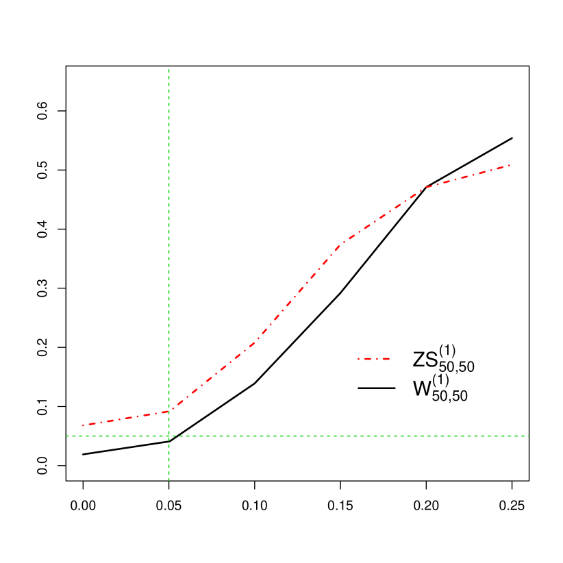
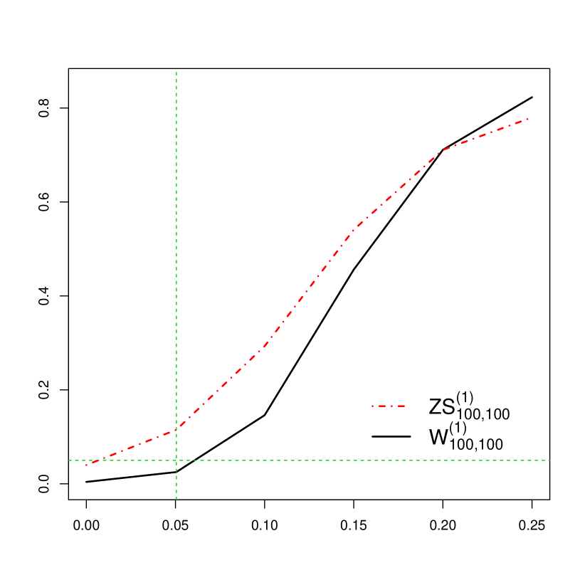
Figure 3.1: Percentage of rejections (out of 1,000 simulations) of the self-normalized statistic of Zhang and Shao, (2015) for the classical hypotheses (3.1) (denoted $ZS_{n,m}^{(1)}$) and the new test (2.13) for the relevant hypohteses (2.3) (denoted by $W^{(1)}_{m,n}$) as a function of $\delta_{1}$ in Scenario 1. In the left hand panel $n=m=50$, and in the right hand panel $n=m=100$. The horizontal green line is at the nominal level 0.05, and the vertical green line at $\delta_{1}=0.05$ indicates the case when $\|v_{1}^{X}-v_{1}^{Y}\|^{2}=\Delta_{1}=0.1.$

.

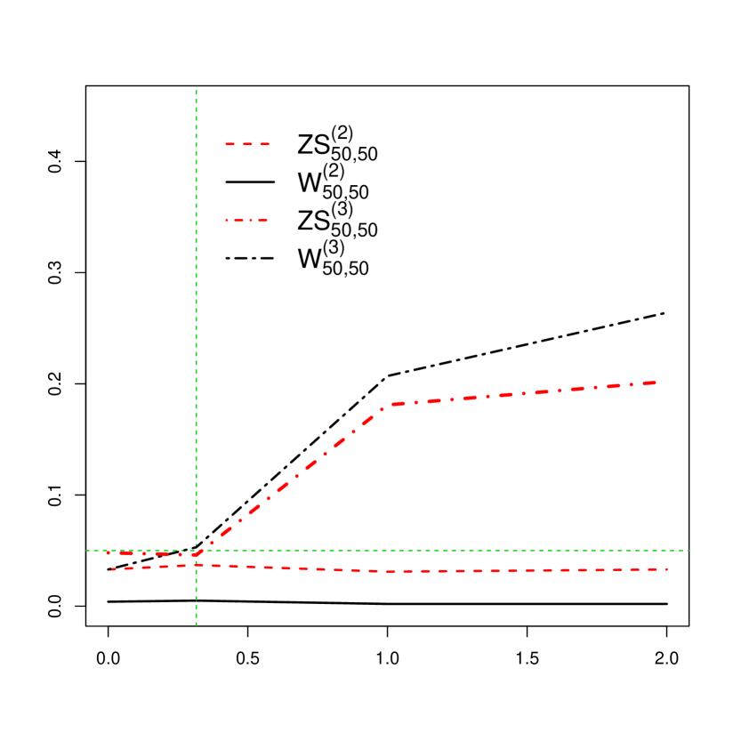
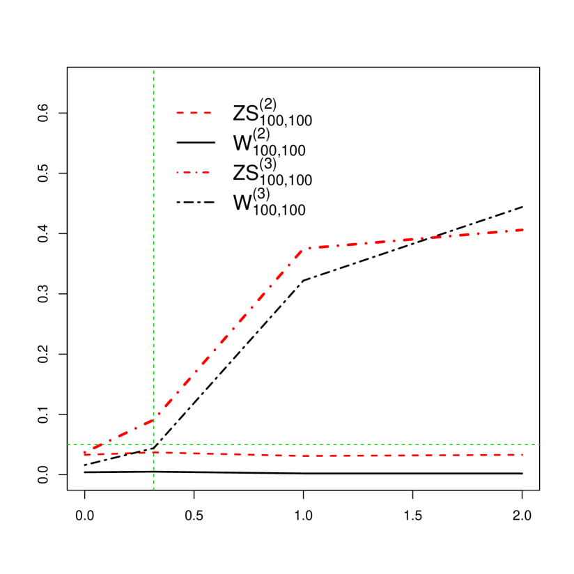
Figure 3.2: Percentage of rejections (out of 1,000 simulations) of the self-normalized statistic of Zhang and Shao, (2015) for the classical hypotheses (3.1) (denoted $ZS_{n,m}^{(j)}$, $j=2,3$) and the new test (2.13) for the relevant hypohteses (2.3) (denoted by $W^{(j)}_{m,n}$, $j=2,3$) as a function of $\delta_{2}$ in Scenario 2. In the left hand panel $n=m=50$, and in the right hand panel $n=m=100$. The horizontal green line is at the nominal level 0.05, and the vertical green line at $\delta_{2}=0.3155$ indicates the case when $\|v_{3}^{X}-v_{3}^{Y}\|^{2}=\Delta_{1}=0.1$.

3.1 Multiple comparisons

In order to investigate the multiple testing procedure of Section 2.3, $X$ and $Y$ samples were generated according to model (3.2) with $n=m=100$ in two situations: one with $\delta_{1}=0.0504915$ and $\delta_{2}=0.3155$, and another with $\delta_{1}=0.25$ and $\delta_{2}=2$. In the former case, $\|v_{j}^{X}-v_{j}^{Y}\|^{2}\approx 0.1$ for $j=1,\ldots,4$, while in the latter case $\|v_{j}^{X}-v_{j}^{Y}\|^{2}>0.1$, $j=1,\ldots,4$. We then applied tests of $H_{0,p}$ in (3.1) with $\Delta_{j}=0.1$ for $j=1,\ldots,4$ and varied $p=1,\ldots,4$. These tests were carried out by combining the marginal tests for relevant differences of the respective eigenfunctions using the standard Bonferroni correction as well as the Holm–Bonferroni correction. Empirical size and power calculated from 1,000 simulations with nominal size $0.05$ for each value of $p$ and correction are reported in Table 3.1. It can be seen that these corrections controlled the family-wise error rate well. The tests still retain similar power when comparing up to four eigenfunctions, although one may notice the declining power as the number of tests increases.

$\delta_{1}$	$\delta_{2}$		$j=1$	$2$	$3$	$4$
0.0504915	0.3155	B	0.036	0.021	0.018	0.017
		HB	0.037	0.036	0.024	0.025
0.25	2	B	0.750	0.678	0.668	0.564
		HB	0.750	0.798	0.716	0.594

Table 3.1: Rejection rates from 1,000 simulations of tests $H_{0,j}$ with nominal level $0.05$ for $j=1,\ldots,4$ and Bonferroni (B) and Holm–Bonferroni (HB) corrections.

4 Application to Australian annual temperature profiles

To demonstrate the practical use of the tests proposed above, the results of an application to annual minimum temperature profiles are presented next. These functions were constructed from data collected at various measuring stations across Australia. The raw data consisted of approximately daily minimum temperature measurements recorded in degrees Celsius over approximately the last 150 years at six stations, and is available in the R package fChange, see Sönmez et al., (2017), as well as from www.bom.gov.au. The exact station locations and time periods considered are summarized in Table 4.1. In addition, Figure 4.1 provides a map of eastern Australia showing the relative locations of these stations.

Location	Years
Sydney, Observatory Hill	1860–2011  (151)
Melbourne, Regional Office	1856–2011  (155)
Boulia, Airport∗	1900–2009  (107)
Gayndah, Post Office	1905–2008  (103)
Hobart, Ellerslie Road	1896–2011  (115)
Robe	1885–2011  (126)

Table 4.1: Locations and names of six measuring stations at which annual temperature data was recorded, and respective observation periods. In brackets are the numbers of available annual temperature profiles. The 1932 and 1970 curves were removed from the Boulia series due to missing values.

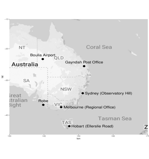
Figure 4.1: Map of eastern Australia showing the locations of the six measuring stations whose data were used in the data analysis. This map was produced using the ggmap package in R; see Kahle and Wickham, (2013).

In each year and for each station, 365 (366 in leap years) raw data points were converted into functional data objects using cubic B-splines at 20 equally spaced knots using the fda package in R; see Ramsay et al., (2009) for details. We also tried using cubic B-splines with between 20 and 40 equally spaced knots, as well as using the same numbers of standard Fourier basis elements to smooth the raw data into functional data objects, and the test results reported below were essentially unchanged. The resulting curves from the stations located in Sydney and Gayndah are displayed respectively in the left and right hand panels of Figure 4.2 as rainbow plots, with earlier curves drawn in red and progressing through the color spectrum to later curves drawn in violet; see Shang and Hyndman, (2016). One may notice that the curves appear to generally increase in level over the years. In order to remove this trend, a linear time trend was estimated for the series of average yearly minimum temperatures, and then this linear trend was subtracted pointwise from the time series of curves. The detrended Sydney and Gayndah curves are displayed again as rainbow plots in the left and right-hand panels of Figure 4.3, which appear to be fairly stationary.

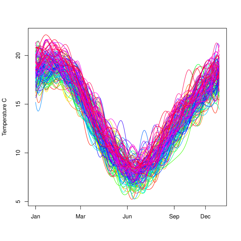
Figure 4.2: Rainbow plots of minimum temperature profiles based on data collected at the Sydney (left panel) and Gayndah (right panel) stations constructed using cubic B-splines.

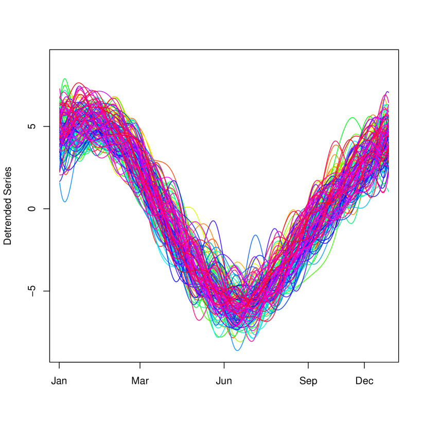
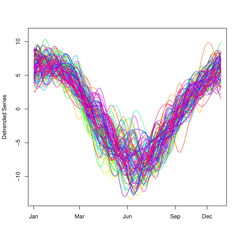
Figure 4.3: Rainbow plots of detrended minimum temperature profiles from Sydney (left panel) and Ganydah (right panel). Detrending was carried out by fitting a linear time trend to the series of average yearly minimum temperatures, and then removing this trend pointwise from the time series of curves.

We took as the goal of the analysis to evaluate whether or not there are relevant differences in the primary modes of variability of these curves between station locations, as measured by differences in the leading eigenfunctions of the sample covariance operators. We applied tests of $H_{0}^{(1)}$ and $H_{0}^{(2)}$ with thresholds $\Delta_{1}=\Delta_{2}=0.1$ based on the statistics $\hat{\mathbb{W}}^{(j)}_{m,n}$, $j=1,2$, to each pair of functional time series from the six stations. The results of these tests are reported in terms of $P$-values in Table 4.2. Plots of the estimated leading eigenfunctions from each sample are displayed in Figure 4.4.

One observes in five out of six stations, excluding the Gayndah station, that the leading eigenfunction of the sample covariances operators is approximately constant, suggesting that the primary mode of variability of those temperature profiles is essentially level fluctuations around the increasing trend. Pairwise comparisons based on tests of $H_{0}^{(1)}$ suggest that these functions in general do not exhibit relevant differences to any reasonable significance. In contrast, the leading eigenfunction calculated from the Gayndah station curves evidently puts more mass in the winter months than the summer months. This is almost expected given the comparison of the detrended curves in Figure 4.3, in which the Gayndah curves evidently exhibit more variability in the winter months relative to the Sydney curves. Pairwise comparisons of the Gayndah data with the other stations suggest that this difference is significant, and even that the change is relevant to the level $\Delta_{1}=0.1$. The analysis of the second eigenfunction leads to a similar conclusion here: the stations other than Gayndah have similar eigenfunction structure, and the curves calculated from the Gayndah station have different eigenfunction structure. However, for the second eigenfunction conclusions about the uniqueness of the Gayndah station cannot be made with the same level of confidence as for the first eigenfuction.

$H_{0}^{(1)},\;\Delta_{1}=0.1$
	Melbourne	Boulia	Gayndah	Hobart	Robe
Sydney	0.2075	0.4545	0.0327	0.2211	0.5614
Melbourne		0.1450	0.0046	0.5007	0.2203
Boulia			0.0466	0.0321	0.5419
Gayndah				0.0002	0.0011
Hobart					0.0885
$H_{0}^{(2)},\;\Delta_{2}=0.1$
	Melbourne	Boulia	Gayndah	Hobart	Robe
Sydney	0.1712	0.0708	0.0865	0.1201	0.0785
Melbourne		0.0862	0.0082	0.1502	0.1778
Boulia			0.0542	0.0553	0.1438
Gayndah				0.0371	0.0037
Hobart					0.4430

Table 4.2: Approximate $P$-values of tests of $H_{0}^{(1)}$ and $H_{0}^{(2)}$ with $\Delta_{1}=\Delta_{2}=0.1$ for all pairwise comparisons of the series of curves from each of the six monitoring stations. Values that are less than 0.05 are bolded.

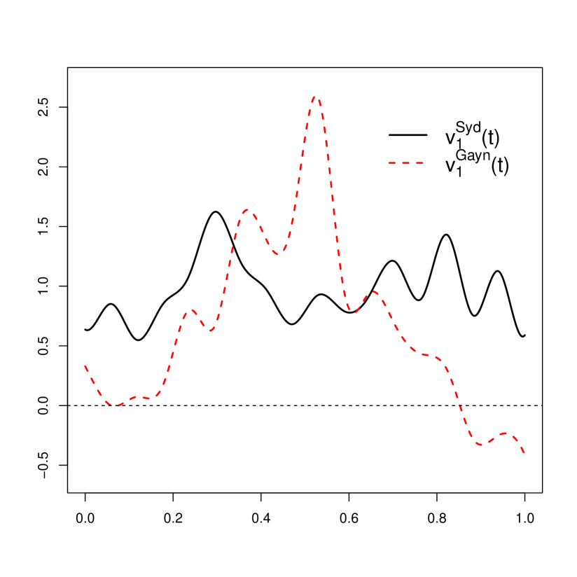
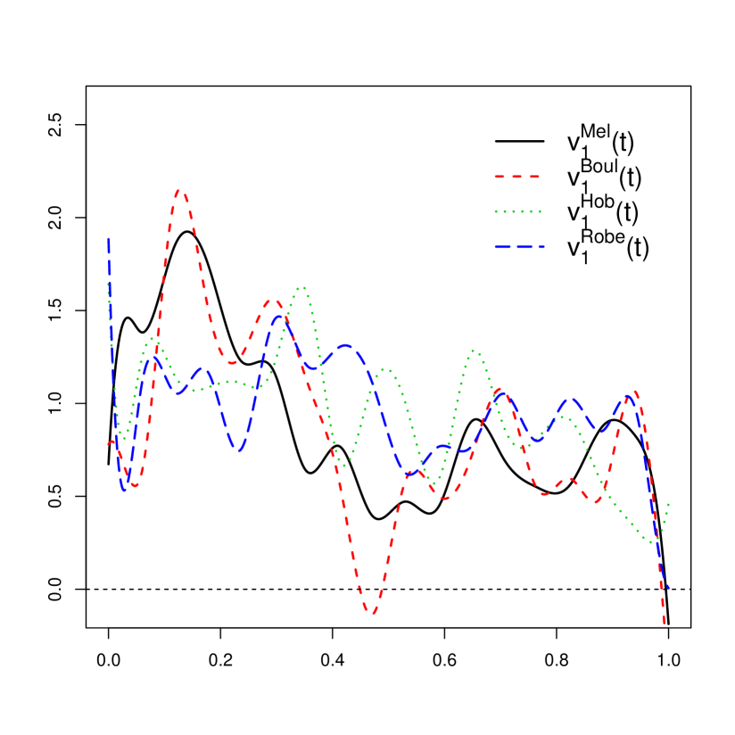
Figure 4.4: Left panel: Plot of sample eigenfunctions corresponding to the largest eigenvalue of the sample covariance operators of the Sydney and Gayndah detrended minimum temperature profiles, $\hat{v}_{1}^{\rm Syd}$ and $\hat{v}_{1}^{\rm Gayn}$. A test of $H_{0}^{(1)}$ suggests that the squared norm of the difference between these curves is significantly larger than 0.1 (P-value $\approx 0.0327$). Right panel: Plots of sample eigenfunctions corresponding to the largest eigenvalues of the sample covariance operators from the remaining four stations.

5 Conclusions

In this paper, new two-sample tests were introduced to detect relevant differences in the eigenfunctions and eigenvectors of covariance operators of two independent functional time series. These tests can be applied both marginally and, with Bonferroni-type corrections, jointly. The tests are constructed utilizing a self-normalizing strategy, leading to an intricate theoretical analysis to derive the large-sample behavior of the proposed tests. Finite-sample evaluations, done through a simulation study and an application to annual minimum temperature data from Australia, highlight that the tests have very good finite sample properties and exhibit the features predicted by the theory.

6 Technical details

In this section we provide the technical details required for the arguments given in Section 2.2.

6.1 Proof of Proposition 2.1

Below let $\int:=\int_{0}^{1}$ for brevity. According to the definitions of $\hat{\tau}^{X}_{j}(\lambda),\hat{v}^{X}_{j}(t,\lambda),\tau^{X}_{j},$ and $v^{X}_{j}$, a simple calculation shows that for almost all $t\in[0,1]$,

$$\int(C^{X}(t,s) +(\hat{C}_{m}^{X}(t,s,\lambda)-C^{X}(t,s)))(v^{X}_{j}(s)+(\hat{v}^{X}_{j}(s,\lambda)-v^{X}_{j}(s)))ds$$ (6.1)

$$=(\tau^{X}_{j}+(\hat{\tau}^{X}_{j}(\lambda)-\tau^{X}_{j}))(v^{X}_{j}(t)+(\hat{v}^{X}_{j}(t,\lambda)-v^{X}_{j}(t))).$$

The sequence $\{v^{X}_{j}\}_{i\in\mathbb{N}}$ forms an orthonormal basis of $L^{2}([0,1])$, and hence there exist coefficients $\{\xi_{j,\lambda}\}_{j\in\mathbb{N}}$ such that

$$\hat{v}^{X}_{j}(t,\lambda)-v^{X}_{j}(t)=\sum_{i=1}^{\infty}\xi_{i,\lambda}v^{X}_{i}(t),$$ (6.2)

for almost every $t$ in $[0,1]$. By rearranging terms in (6.1), we see that

$$\int C^{X}(t,s)(\hat{v}^{X}_{j}(s,\lambda) -v^{X}_{j}(s))ds+\int\left(\hat{C}_{m}^{X}(t,s,\lambda)-C^{X}(t,s)\right)v^{X}_{j}(s)ds$$ (6.3)

$$=\tau^{X}_{j}(\hat{v}^{X}_{j}(t,\lambda)-v^{X}_{j}(t))+\left(\hat{\tau}^{X}_{j}(\lambda)-\tau^{X}_{j}\right)v^{X}_{j}(t)+G_{j,m}(t,\lambda),$$

where

$$G_{j,m}(t,\lambda)=\int[C^{X}(t,s)-\hat{C}_{m}^{X}(t,s,\lambda)][\hat{v}^{X}_{j}(s,\lambda)-v^{X}_{j}(s)]ds+[\hat{\tau}^{X}_{j}(\lambda)-\tau^{X}_{j}][\hat{v}^{X}_{j}(t,\lambda)-v^{X}_{j}(t)].$$

Taking the inner product on the left and right hand sides of (6.3) with $v_{k}$, for $k\neq i$, and employing (6.2) yields

$$\tau^{X}_{k}\xi_{k,\lambda}+\int\int\left(\hat{C}_{m}^{X}(t,s,\lambda)-C^{X}(t,s)\right)v^{X}_{j}(s)v^{X}_{k}(t)dsdt=\tau^{X}_{j}\xi_{k,\lambda}+\langle G_{j,m}(\cdot,\lambda),v^{X}_{k}\rangle,$$

which implies that

$$\xi_{k,\lambda}=\frac{\langle\hat{C}_{m}^{X}(\cdot,\cdot,\lambda)-C^{X},v^{X}_{j}\otimes v^{X}_{k}\rangle}{\tau^{X}_{j}-\tau^{X}_{k}}-\frac{\langle G_{j,m}(\cdot,\lambda),v^{X}_{k}\rangle}{\tau^{X}_{j}-\tau^{X}_{k}},$$ (6.4)

for all ${\lambda\in[0,1]}$ and $k\neq i$. Furthermore, by the parallelogram law,

$$\xi_{i,\lambda}=\langle v^{X}_{j},\hat{v}^{X}_{j}(\cdot,\lambda)-v^{X}_{j}\rangle=-\frac{1}{2}\|\hat{v}^{X}_{j}(\cdot,\lambda)-v^{X}_{j}\|^{2}.$$ (6.5)

Let $S_{j,X}=\min\{\tau_{j-1}^{X}-\tau_{j}^{X},\tau_{j}^{X}-\tau_{j+1}^{X}\}$ for $j\geq 2$ and $S_{1,X}=\tau_{1}^{X}-\tau_{2}^{X}$. By Assumption 2.3 and the fact that $j\leq d$ we have $S_{j,X}>0$. Hence, Lemma 2.2 in Horváth and Kokoszka, (2012) (see also Section 6.1 of Gohberg et al., (1990)) implies for all $\lambda\in[0,1]$,

$$\sqrt{\lambda}\|\hat{v}^{X}_{j}(\cdot,\lambda)-v^{X}_{j}\|\leq\frac{1}{S_{j,X}}\big{\|}\sqrt{\lambda}[\hat{C}_{m}^{X}(\cdot,\cdot,\lambda)-C^{X}]\big{\|}.$$ (6.6)

Further,

$$\sqrt{\lambda}[\hat{C}_{m}^{X}(t,s,\lambda)-C^{X}(t,s)] =\frac{\sqrt{\lambda}}{\lfloor m\lambda\rfloor}\sum^{\lfloor m\lambda\rfloor}_{i=1}(X_{i}(t)X_{i}(s)-C^{X}(t,s))$$

$$=\frac{1}{\sqrt{m}}\frac{\sqrt{m\lambda}}{\sqrt{\lfloor m\lambda\rfloor}}\frac{1}{\sqrt{\lfloor m\lambda\rfloor}}\sum^{\lfloor m\lambda\rfloor}_{i=1}(X_{i}(t)X_{i}(s)-C^{X}(t,s)).$$

It is easy to show using Cauchy–Schwarz inequality that the sequence $X_{i}(\cdot)X_{i}(\cdot)-C^{X}(\cdot,\cdot)\in L^{2}([0,1])^{2}$ is $L^{2+\kappa}$-$m$-approximable for some $\kappa>0$ if $X_{i}$ is $L^{p}$-$m$-approximable for some $p>4$. Lemma B.1 from the Supplementary Material of Aue et al., 2018a can be generalized to $L^{2+\kappa}$-$m$-approximable random variables taking values in $L^{2}([0,1]^{2})$, from which it follows that

$$\sup_{\lambda\in[0,1]}\frac{1}{\sqrt{\lfloor m\lambda\rfloor}}\Big{\|}\sum^{\lfloor m\lambda\rfloor}_{i=1}(X_{i}(\cdot)X_{i}(\cdot)-C^{X}(\cdot,\cdot))\Big{\|}=O_{\mathbb{P}}(\log^{(1/\kappa)}(m)).$$

Using this and combining with (6.6), we obtain the bound

$$\sup_{\lambda\in[0,1]}\Big{\|}\sqrt{\lambda}[\hat{C}_{m}^{X}(\cdot,\cdot,\lambda)-C^{X}]\Big{\|}O_{\mathbb{P}}\Big{(}{\log^{(1/\kappa)}(m)}{\sqrt{m}}\Big{)},$$ (6.7)

and the estimate (2.31). Furthermore, using the bound that

$$|\hat{\tau}^{X}_{j}(\lambda)-\tau^{X}_{j}|\leq\big{\|}\hat{C}_{m}^{X}(\cdot,\cdot,\lambda)-C^{X}\big{\|},$$

we obtain by similar arguments that

$$\sup_{\lambda\in[0,1]}\sqrt{\lambda}|\hat{\tau}^{X}_{j}(\lambda)-\tau^{X}_{j}|=O_{\mathbb{P}}\Big{(}\frac{\log^{(1/\kappa)}(m)}{\sqrt{m}}\Big{)}.$$ (6.8)

Using the triangle inequality, Cauchy–Schwarz inequality, and combining (6.7) and (6.8), it follows

$$\sup_{\lambda\in[0,1]}\lambda\|G_{j,m}(\cdot,\lambda)\|\leq \sqrt{\lambda}\Big{\|}[\hat{C}_{m}^{X}(\cdot,\cdot,\lambda)-C^{X}]\Big{\|}\sup_{\lambda\in[0,1]}\sqrt{\lambda}\|\hat{v}(\cdot,\lambda)-v^{X}_{j}\|$$ (6.9)

$$+\sup_{\lambda\in[0,1]}\sqrt{\lambda}|\hat{\tau}^{X}_{j}(\lambda)-\tau^{X}_{j}|\sup_{\lambda\in[0,1]}\sqrt{\lambda}\|\hat{v}(\cdot,\lambda)-v^{X}_{j}\|=O_{\mathbb{P}}\Big{(}\frac{\log^{(2/\kappa)}(m)}{m}\Big{)}.$$

Let

$$R_{i,m}(t,\lambda)=\frac{1}{\sqrt{m}}\sum_{k\neq i}\frac{v^{X}_{k}(t)}{\tau^{X}_{j}-\tau^{X}_{k}}\int^{1}_{0}\hat{Z}^{X}_{m}(s_{1},s_{2},\lambda)v^{X}_{k}(s_{2})v^{X}_{j}(s_{1})ds_{1}ds_{2}.$$

Combining (6.2), (6.4) and (6.5), we see that for almost all $t\in[0,1]$ and for all $\lambda\in[0,1]$,

$$\lambda[\hat{v}^{X}_{j}(\cdot,\lambda)-v^{X}_{j}(t)]=\frac{m\lambda}{\lfloor m\lambda\rfloor}R_{i,m}(t,\lambda)-\sum_{k\neq i}\frac{\langle\lambda G_{j,m}(\cdot,\lambda),v^{X}_{k}\rangle}{\tau^{X}_{j}-\tau^{X}_{k}}v^{X}_{k}(t)-\frac{1}{2}\|\hat{v}^{X}_{j}(\cdot,\lambda)-v^{X}_{j}\|^{2}v_{j}^{X}(t),$$

with the convention that $({m\lambda}/{\lfloor m\lambda\rfloor})R_{i,m}(t,\lambda)=0$ for $\lambda<1/m$. Using this identity and the triangle inequality, we obtain

$$\sup_{\lambda\in[0,1]}\Big{\|} \lambda[\hat{v}^{X}_{j}(\cdot,\lambda)-v^{X}_{j}(t)]-\frac{m\lambda}{\lfloor m\lambda\rfloor}R_{i,m}(t,\lambda)\Big{\|}$$ (6.10)

$$\leq\frac{1}{2}\sup_{\lambda\in[0,1]}\lambda\|\hat{v}^{X}_{j}(\cdot,\lambda)-v^{X}_{j}\|^{2}+\sup_{\lambda\in[0,1]}\Big{\|}\sum_{k\neq i}\frac{\langle\lambda G_{j,m}(\cdot,\lambda),v^{X}_{k}\rangle}{\tau^{X}_{j}-\tau^{X}_{k}}v^{X}_{k}(t)\Big{\|}.$$

The first term on the right-hand side of (6.10) can be bounded by bound (2.31). In order to bound the second term we have, using the orthonormality of the $v^{X}_{k}$ (Parseval’s identity) and the fact that $1/(\tau^{X}_{j}-\tau^{X}_{k})^{2}\leq 1/S_{j,X}^{2}$ for all $k\neq i$, that

$$\Big{\|}\sum_{k\neq i}\frac{\langle\lambda G_{j,m}(\cdot,\lambda),v^{X}_{k}\rangle}{\tau^{X}_{j}-\tau^{X}_{k}}v^{X}_{k}(\cdot)\Big{\|} =\Big{(}\sum_{k\neq i}\frac{\langle\lambda G_{j,m}(\cdot,\lambda),v^{X}_{k}\rangle^{2}}{(\tau^{X}_{j}-\tau^{X}_{k})^{2}}\Big{)}^{1/2}$$

$$\leq\frac{1}{S_{j,X}}\Big{(}\sum_{k\neq i}{\langle\lambda G_{j,m}(\cdot,\lambda),v^{X}_{k}\rangle^{2}}\Big{)}^{1/2}\leq\frac{1}{S_{j,X}}\|\lambda G_{j,m}(\cdot,\lambda)\|.$$

Therefore

$$\sup_{\lambda\in[0,1]}\Big{\|}\sum_{k\neq i}\frac{\langle\lambda G_{j,m}(\cdot,\lambda),v^{X}_{k}\rangle}{\tau^{X}_{j}-\tau^{X}_{k}}v^{X}_{k}(\cdot)\Big{\|} \leq\sup_{\lambda\in[0,1]}\frac{1}{S_{j,X}}\|\lambda G_{j,m}(\cdot,\lambda)\|=O_{\mathbb{P}}\Big{(}\frac{\log^{(2/\kappa)}(m)}{m}\Big{)},$$

where the last estimate follows from (6.9). Using these bounds in (6.10), we obtain that

$$\sup_{\lambda\in[0,1]}\Big{\|}\lambda[\hat{v}^{X}_{j}(\cdot,\lambda)-v^{X}_{j}(t)]-\frac{m\lambda}{\lfloor m\lambda\rfloor}R_{i,m}(t,\lambda)\Big{\|}=O_{\mathbb{P}}\Big{(}\frac{\log^{(2/\kappa)}(m)}{m}\Big{)}.$$

Given the convention that $({m\lambda}/{\lfloor m\lambda\rfloor})R_{i,m}(t,\lambda)=0$ for $0\leq\lambda<1/m$, the result follows then by showing that

$$\sup_{\lambda\in[1/m,1]}\Big{|}\frac{m\lambda}{\lfloor m\lambda\rfloor}-1\Big{|}\Big{\|}R_{i,m}(t,\lambda)\Big{\|}=O_{\mathbb{P}}\Big{(}\frac{\log^{(2/\kappa)}(m)}{m}\Big{)}.$$

This result is a consequence of $\sup_{\lambda\in[1/m,1]}\big{|}\frac{m\lambda}{\lfloor m\lambda\rfloor}-1\big{|}\leq 1/m$, and $\sup_{\lambda\in[1/m,1]}\|R_{i,m}(t,\lambda)\|=O_{\mathbb{P}}(1)$.

6.2 Proof of Proposition 2.3

Before proceeding with this proof, we develop some notation as well as a rigorous definition of the constant $\zeta_{j}$. Recall the notations (2.34), (2.29) and (2.30) and define the random variables

$$\tilde{X}_{i}(s_{1},s_{2})=X_{i}(s_{1})X_{i}(s_{2})-C^{X}(s_{1},s_{2});\quad\tilde{Y}_{i}(s_{1},s_{2})=Y_{i}(s_{1})Y_{i}(s_{2})-C^{Y}(s_{1},s_{2}).$$ (6.11)

Further let the random variables $\overline{X}_{i}^{(j)}$ and $\overline{Y}_{i}^{(j)}$ be defined by

$$\overline{X}_{i}^{(j)}=\int^{1}_{0}\tilde{X}_{i}(s_{1},s_{2})f^{X}_{j}(s_{1},s_{2})ds_{1}ds_{2}~{},~{}\overline{Y}_{i}^{(j)}=\int^{1}_{0}\tilde{Y}_{i}(s_{1},s_{2})f^{Y}_{j}(s_{1},s_{2})ds_{1}ds_{2},$$ (6.12)

with the functions $f^{X}_{j},f^{Y}_{j}$ given by

$$f^{X}_{j}(s_{1},s_{2}) = -v^{X}_{j}(s_{1})\sum_{k\neq j}\frac{v^{X}_{k}(s_{2})}{\tau^{X}_{j}-\tau^{X}_{k}}\int^{1}_{0}v^{X}_{k}(t)v^{Y}_{j}(t)dt,$$ (6.13)

$$f^{Y}_{j}(s_{1},s_{2}) = -v^{Y}_{j}(s_{1})\sum_{k\neq j}\frac{v^{Y}_{k}(s_{2})}{\tau^{Y}_{j}-\tau^{Y}_{k}}\int^{1}_{0}v^{Y}_{k}(t)v^{X}_{j}(t)dt.$$ (6.14)

Firstly, we note that by using the orthonormality of the eigenfunctions $v_{j}^{X}$ and $v_{j}^{Y}$, and Assumption 2.3, we get that

$$\|f^{X}_{j}\|^{2}=\int\int(f^{X}_{j}(s_{1},s_{2}))^{2}ds_{1}ds_{2}=\|v_{j}^{X}\|^{2}\sum_{k\neq j}\frac{\left(\int^{1}_{0}v^{X}_{k}(t)v^{Y}_{j}(t)dt\right)^{2}}{(\tau^{X}_{j}-\tau^{X}_{k})^{2}}\leq 1/S_{j,X}^{2}<\infty.$$

Let

$$\sigma_{X,j}^{2}=\sum_{\ell=-\infty}^{\infty}\mbox{cov}(\overline{X}_{0}^{(j)},\overline{X}_{\ell}^{(j)}),\mbox{~{}~{} and ~{}~{}}\sigma_{Y,j}^{2}=\sum_{\ell=-\infty}^{\infty}\mbox{cov}(\overline{Y}_{0}^{(j)},\overline{Y}_{\ell}^{(j)}).$$

Based on these quantities, $\zeta_{j}$ is defined as

$$\zeta_{j}=2\sqrt{\frac{\sigma_{X,j}^{2}}{\theta}+\frac{\sigma_{Y,j}^{2}}{1-\theta}}.$$ (6.15)

Proof of Proposition 2.3.

We can write

$$\hat{Z}^{(j)}_{m,n}(\lambda) = \sqrt{m+n}\int^{1}_{0}(\hat{D}^{(j)}_{m,n}(t,\lambda))^{2}-\lambda^{2}D^{2}_{j}(t))dt$$

$$= \sqrt{m+n}\ \Big{\{}\int^{1}_{0}(\hat{D}^{(j)}_{m,n}(t,\lambda)-\lambda D_{j}(t))^{2}+2\lambda D_{j}(t)(\hat{D}^{(j)}_{m,n}(t,\lambda)-\lambda D_{j}(t))^{2}dt$$

$$= \sqrt{m+n}\int^{1}_{0}(\tilde{D}^{(j)}_{m,n}(t,\lambda))^{2}dt+2\lambda\sqrt{m+n}\int^{1}_{0}D_{j}(t)\tilde{D}_{m,n}^{(j)}(t,\lambda)dt+o_{\mathbb{P}}(1)$$

uniformly with respect to $\lambda\in[0,1]$, where the process $\tilde{D}_{m,n}^{(j)}(t,\lambda)$ is defined in (2.34) and Proposition 2.2 was used in the last equation. Observing (2.35) gives

$$\hat{Z}^{(j)}_{m,n}(\lambda)=\tilde{Z}^{(j)}_{m,n}(\lambda)+o_{\mathbb{P}}(1)$$ (6.17)

uniformly with respect to $\lambda\in[0,1]$, where the process $\tilde{Z}_{m,n}^{(j)}$ is given by

$$\tilde{Z}^{(j)}_{m,n}(\lambda)=2\lambda\sqrt{m+n}\int^{1}_{0}D_{j}(t)\tilde{D}^{(j)}_{m,n}(t,\lambda)dt.$$ (6.18)

Consequently the assertion of Proposition 2.3 follows from the weak convergence

$$\{\tilde{Z}^{(j)}_{m,n}(\lambda)\}_{\lambda\in[0,1]}\rightsquigarrow\{\lambda\zeta_{j}\mathbb{B}(\lambda)\}_{\lambda\in[0,1]}.$$

We obtain, using the orthogonality of the eigenfunctions and the notation (2.6), that

$$\tilde{Z}^{(j)}_{m,n}(\lambda) = 2\lambda\sqrt{m+n}\Big{\{}\frac{1}{\sqrt{m}}\int^{1}_{0}\hat{Z}^{X}_{m}(s_{1},s_{2},\lambda)\int^{1}_{0}D_{j}(t)\sum_{k\neq j}\frac{v^{X}_{k}(t)}{\tau^{X}_{j}-\tau^{X}_{k}}dtv^{X}_{j}(s_{1})v^{X}_{k}(s_{2})ds_{1}ds_{2}$$ (6.19)

$$-\frac{1}{\sqrt{n}}\int^{1}_{0}Z^{Y}_{n}(s_{1},s_{2},\lambda)\int^{1}_{0}D_{j}(t)\sum_{k\neq j}\frac{v^{Y}_{k}(t)}{\tau^{Y}_{j}-\tau^{Y}_{k}}dtv^{Y}_{j}(s_{1})v^{Y}_{k}(s_{2})ds_{1}ds_{2}\Big{\}}$$

$$= 2\lambda\sqrt{m+n}\Big{\{}\frac{1}{m}\sum_{i=1}^{\lfloor m\lambda\rfloor}\overline{X}_{i}^{(j)}+\frac{1}{n}\sum_{i=1}^{\lfloor n\lambda\rfloor}Y_{i}^{(j)}\Big{\}},$$

where the random variables $\overline{X}_{i}^{(j)}$ and $\bar{Y}_{i}^{(j)}$ are defined above. We now aim to establish that

$$\Big{\{}\frac{1}{\sqrt{m}}\sum_{i=1}^{\lfloor m\lambda\rfloor}\overline{X}_{i}^{(j)}\Big{\}}_{\lambda\in[0,1]}\rightsquigarrow\sigma_{X,j}\{\mathbb{B}^{X}(\lambda)\}_{\lambda\in[0,1]},$$ (6.20)

where $\mathbb{B}^{X}$ is a standard Brownian motion on the interval $[0,1]$. In the following we use the symbol $\|\cdot\|$ simultaneously for $L^{2}$-norm on the space $L^{2}([0,1])$ and $L^{2}([0,1]^{2})$ as the particular meaning is always clear from the context. Firstly, we note that by using the orthonormality of the eigenfunctions $v_{j}^{X}$ and $v_{j}^{Y}$, and Assumption 2.3, we get that

$$\|f^{X}_{j}\|^{2}=\int\int(f^{X}_{j}(s_{1},s_{2}))^{2}ds_{1}ds_{2}=\|v_{j}^{X}\|^{2}\sum_{k\neq j}\frac{\left(\int^{1}_{0}v^{X}_{k}(t)v^{Y}_{j}(t)dt\right)^{2}}{(\tau^{X}_{j}-\tau^{X}_{k})^{2}}\leq 1/S_{j,X}^{2}<\infty.$$

The following calculation is similar to Lemma A.3 in Aue et al., 2018b . Let

$$\tilde{X}_{i}^{(m)}(t,s)=X_{i,m}(t)X_{i,m}(s)-\mathbb{E}X_{0}(t)X_{0}(s),$$

where $\{X_{i,m}\}_{i\in\mathbb{Z}}$ is the mean zero $m$-dependent sequence used in definition of $m$-approximability (see Assumption 2.2). Moreover, if $q=p/2$ with $p$ given in Assumption 2.2, then we have by the triangle inequality and Minkowski’s inequality that

$$\big{\{}\mathbb{E}\|\tilde{X}_{i}-\tilde{X}_{i}^{(m)}\|^{q}\big{\}}^{1/q} \leq\big{\{}\mathbb{E}(\|X_{i}(\cdot)(X_{i}(\cdot)-X_{i,m}(\cdot))\|+\|X_{i,m}(\cdot)(X_{i}(\cdot)-X_{i,m}(\cdot))\|)^{q}\big{\}}^{1/q}$$ (6.21)

$$\leq\big{\{}\mathbb{E}(\|X_{i}(\cdot)(X_{i}(\cdot)-X_{i,m}(\cdot))\|^{q}\big{\}}^{1/q}+\big{\{}\mathbb{E}\|X_{i,m}(\cdot)(X_{i}(\cdot)-X_{i,m}(\cdot))\|^{q}\big{\}}^{1/q}.$$

Using the definition of the norm in $L^{2}([0,1])$, it is clear that

$$\|X_{i}(\cdot)(X_{i}(\cdot)-X_{i,m}(\cdot))\|=\|X_{i}\|\|X_{i}-X_{i,m}\|,$$

and hence we obtain from the Cauchy–Schwarz inequality applied to the expectation on the concluding line of (6.21) and stationarity that

$$(\mathbb{E}(\|X_{i}(\cdot)(X_{i}(\cdot)-X_{i,m}(\cdot))\|^{q})^{1/q}+(\mathbb{E} \|X_{i,m}(\cdot)(X_{i}(\cdot)-X_{i,m}(\cdot))\|^{q})^{1/q}$$

$$\leq(\mathbb{E}\|X_{0}\|^{2q})^{1/2q}(\mathbb{E}\|X_{0}-X_{0,m}\|^{2q})^{1/2q}.$$

It follows from this and (6.21) that

$$\sum_{m=1}^{\infty}(\mathbb{E}\|\tilde{X}_{i}-\tilde{X}_{i}^{(m)}\|^{q})^{1/q}\leq(\mathbb{E}\|X_{0}\|^{p})^{1/p}\sum_{m=1}^{\infty}(\mathbb{E}\|X_{0}-X_{0,m}\|^{p})^{1/p}<\infty.$$ (6.22)

Now let $\overline{X}_{i,m}^{(j)}$ be defined as $\overline{X}_{i}^{(j)}$ in (6.12) with $X_{i}$ replaced by $X_{i,m}$. We obtain using the Cauchy–Schwarz inequality that

$$(\mathbb{E}[\overline{X}_{i}^{(j)}-\overline{X}_{i,m}^{(j)}]^{q})^{1/q}\leq\|f^{X}_{j}\|(\mathbb{E}\|\tilde{X}_{i}-\tilde{X}_{i}^{(m)}\|^{q})^{1/q}.$$

By (6.22) it follows that

$$\sum_{m=1}^{\infty}(\mathbb{E}[\overline{X}_{i}^{(j)}-\overline{X}_{i,m}^{(j)}]^{q})^{1/q}<\infty$$

and therefore the sequence $\overline{X}_{i}^{(j)}$ satisfies the assumptions of Theorem 3 in Wu, (2005). By this result the weak convergence in (6.20) follows. By the same arguments it follows that

$$\Big{\{}\frac{1}{\sqrt{n}}\sum_{i=1}^{\lfloor n\lambda\rfloor}\overline{Y}_{i}^{(j)}\Big{\}}_{\lambda\in[0,1]}\rightsquigarrow\sigma_{Y,j}\{Ê\mathbb{B}^{Y}(\lambda)\}_{\lambda\in[0,1]},$$ (6.23)

where $\mathbb{B}^{Y}$ is a standard Brownian motion on the interval $[0,1]$ and

$$\sigma_{Y,j}^{2}=\sum_{\ell=-\infty}^{\infty}\mbox{cov}(\overline{Y}_{0}^{(j)},\overline{Y}_{\ell}^{(j)}).$$

Since the sequences $\{X_{i}\}_{i\in\mathbb{R}}$ and $\{Y_{i}\}_{i\in\mathbb{R}}$ are independent, we have that (6.20) and (6.23) may be taken to hold jointly where the Brownian motions $\mathbb{B}^{X}$ and $\mathbb{B}^{Y}$ are independent. It finally follows from this and (6.19) that

$$\{\tilde{Z}^{(j)}_{m,n}(\lambda)\}_{\lambda\in[0,1]} \rightsquigarrow\Big{\{}2\lambda\Big{(}\frac{\sigma_{X,j}}{\sqrt{\theta}}\mathbb{B}^{X}(\lambda)+\frac{\sigma_{Y,j}}{\sqrt{1-\theta}}\mathbb{B}^{Y}(\lambda)\Big{)}\Big{\}}_{\lambda\in[0,1]}~{}\stackrel{{\scriptstyle\cal D}}{{=}}~{}\big{\{}\lambda\zeta_{j}\mathbb{B}(\lambda)\big{\}}_{\lambda\in[0,1]}~{},$$

which completes the proof of Proposition 2.3. ∎

Acknowledgements This work has been supported in part by the Collaborative Research Center “Statistical modeling of nonlinear dynamic processes” (SFB 823, Teilprojekt A1,C1) of the German Research Foundation (DFG), and the Natural Sciences and Engineering Research Council of Canada, Discovery Grant. We gratefully acknowledge Professors Xiaofeng Shao and Xianyang Zhang for sharing code to reproduce their numerical examples with us.

References

• Aitchison, (1964) Aitchison, J. (1964). Confidence-region tests. Journal of the Royal Statistical Society, Series B, 26:462–476.
• Aston and Kirch, (2012) Aston, J. and Kirch, C. (2012). Estimation of the distribution of change-points with application to fMRI data. The Annals of Applied Statistics, 6:1906–1948.
• Aue et al., (2015) Aue, A., Norinho, D. D., and Hörmann, S. (2015). On the prediction of stationary functional time series. Journal of the American Statistical Association, 110:378–392.
• (4) Aue, A., Rice, G., and Sönmez, O. (2018a). Detecting and dating structural breaks in functional data without dimension reduction. Journal of the Royal Statistical Society, Series B, 80:509–529.
• (5) Aue, A., Rice, G., and Sönmez, O. (2018b). Structural break analysis for spectrum and trace of covariance operators. University of California Davis, Working Paper, URL: https://arxiv.org/abs/1804.03255.
• Benko et al., (2009) Benko, M., Härdle, W., and Kneip, A. (2009). Common functional principal components. The Annals of Statistics, 37:1–34.
• Berkson, (1938) Berkson, J. (1938). Some difficulties of interpretation encountered in the application of the chi-square test. Journal of the American Statistical Association, 33:526–536.
• Bertail et al., (2006) Bertail, P., Doukhan, P., and Soulier, P. (2006). Dependence in Probability and Statistics (Lecture Notes in Statistics 187). Springer, New York.
• Bradley, (2005) Bradley, R. C. (2005). Basic properties of strong mixing conditions. A survey and some open questions. Probability Surveys, 2:107–144.
• Bücher et al., (2019) Bücher, A., Dette, H., and Heinrichs, F. (2019+). Detecting deviations from second-order stationarity in locally stationary functional time series. To appear in: Annals of the Institute of Statistical Mathematics; arXiv:1808.04092.
• Dauxois et al., (1982) Dauxois, J., Pousse, A., and Romain, Y. (1982). Asymptotic theory for the principal component analysis of a vector random function: Some applications to statistical inference. Journal of Multivariate Analysis, 12:136–154.
• Dette et al., (2019) Dette, H., Kokot, K., and Aue, A. (2019+). Functional data analysis in the Banach space of continuous functions. To appear in: The Annals of Statistics.
• Dette et al., (2018) Dette, H., Kokot, K., and Volgushev, S. (2018). Testing relevant hypotheses in functional time series via self-normalization. arXiv:1809.06092.
• Fremdt et al., (2013) Fremdt, S., Steinebach, J. G., Horváth, L., and Kokoskza, P. (2013). Testing the equality of covariance operators in functional samples. Scandinavian Journal of Statistics, 40:138–152.
• Gohberg et al., (1990) Gohberg, I., Goldberg, S., and Kaashoek, M. A. (1990). Classes of Linear Operators. Vol. I. Operator Theory: Advances and Applications 49. Birkhäuser, Basel.
• Guo et al., (2016) Guo, J., Zhou, B., and Zhang, J.-T. (2016). A supremum-norm based test for the equality of several covariance functions. Computational Statistics & Data Analysis, 124.
• Hall and Hosseini-Nasab, (2006) Hall, P. and Hosseini-Nasab, M. (2006). On properties of functional principal components analysis. Journal of the Royal Statistical Society, Series B, 68:109–126.
• Hall and Van Keilegom, (2007) Hall, P. and Van Keilegom, I. (2007). Two-sample tests in functional data analysis starting from discrete data. Statistica Sinica, 17:1511–1531.
• Holm, (1979) Holm, S. (1979). A simple sequentially rejective multiple test procedure. Scandinavian Journal of Statistics, 6:65–70.
• Hörmann and Kokoszka, (2010) Hörmann, S. and Kokoszka, P. (2010). Weakly dependent functional data. The Annals of Statistics, 38:1845–1884.
• Horváth et al., (2013) Horváth, L., Kokoskza, P., and Reeder, R. (2013). Estimation of the mean of functional time series and a two sample problem. Journal of the Royal Statistical Society, Series B, 75:103–122.
• Horváth and Kokoszka, (2012) Horváth, L. and Kokoszka, P. (2012). Inference for Functional Data with Applications. Springer, New York.
• Hyndman and Shang, (2009) Hyndman, R. L. and Shang, H. L. (2009). Forcasting functional time series. Journal of the Korean Statistical Soceity, 38:199–221.
• Kahle and Wickham, (2013) Kahle, D. and Wickham, H. (2013). ggmap: Spatial visualization with ggplot2. The R Journal, 5:144–161.
• Kokoszka and Reimherr, (2013) Kokoszka, P. and Reimherr, M. (2013). Asymptotic normality of the principal components of functional time series. Stochastic Processes and their Applications, 123:1546–1562.
• Kowal et al., (2019) Kowal, D. R., Matteson, D. S., and Ruppert, D. (2019). Functional autoregression for sparsely sampled data. Journal of Business and Economics Statistics, 37:97–109.
• Panaretos et al., (2010) Panaretos, V. M., Kraus, D., and Maddocks, J. H. (2010). Second-order comparison of Gaussian random functions and the geometry of DNA minicircles. Journal of the American Statistical Association, 105:670–682.
• Panaretos and Tavakoli, (2013) Panaretos, V. M. and Tavakoli, S. (2013). Fourier analysis of stationary time series in function space. The Annals of Statistics, 41:568–603.
• Paparoditis and Sapatinas, (2016) Paparoditis, E. and Sapatinas, T. (2016). Bootstrap-based testing of equality of mean functions or equality of covariance operators for functional data. Biometrika, 103:727–733.
• Pigoli et al., (2014) Pigoli, D., Aston, J., Dryden, I., and Secchi, P. (2014). Distances and inference for covariance operators. Biometrika, 101:409–422.
• Pomann et al., (2016) Pomann, G.-M., Staicu, A.-M., and Ghosh, S. (2016). A two-sample distribution-free test for functional data with application to a diffusion tensor imaging study of multiple sclerosis. Journal of the Royal Statistical Society, Series C, 65:395–414.
• R Core Team, (2016) R Core Team (2016). R: A Language and Environment for Statistical Computing. R Foundation for Statistical Computing, Vienna, Austria.
• Ramsay et al., (2009) Ramsay, J., Hooker, G., and Graves, S. (2009). Functional Data Analysis with R and MATLAB. Springer, New York.
• Ramsay and Silverman, (2005) Ramsay, J. and Silverman, B. (2005). Functional Data Analysis. Springer, New York.
• Shang and Hyndman, (2016) Shang, H. L. and Hyndman, R. J. (2016). rainbow: Rainbow Plots, Bagplots and Boxplots for Functional Data. R package version 3.4.
• Shao, (2010) Shao, X. (2010). A self-normalized approach to confidence interval construction in time series. Journal of the Royal Statistical Society, Series B, 72:343–366.
• Shao, (2015) Shao, X. (2015). Self-normalization for time series: A review of recent developments. Journal of the American Statistical Association, 110:1797–1817.
• Shao and Zhang, (2010) Shao, X. and Zhang, X. (2010). Testing for change points in time series. Journal of the American Statistical Association, 105:1228–1240.
• Sönmez et al., (2017) Sönmez, O., Aue, A., and Rice, G. (2017). fChange: Change Point Analysis in Functional Data. R package version 0.2.0.
• Tavakoli and Panaretos, (2016) Tavakoli, S. and Panaretos, V. M. (2016). Detecting and localizing differences in functional time series dynamics: a case study in molecular biophysics. Journal of the American Statistical Association, 111:1020–1035.
• Wellek, (2010) Wellek, S. (2010). Testing Statistical Hypotheses of Equivalence and Noninferiority. CRC Press, Boca Raton, FL.
• Wu, (2005) Wu, W. (2005). Nonlinear System Theory: Another Look at Dependence, volume 102 of Proceedings of The National Academy of Sciences of the United States. National Academy of Sciences.
• Zhang and Shao, (2015) Zhang, X. and Shao, X. (2015). Two sample inference for the second-order property of temporally dependent functional data. Bernoulli, 21:909–929.
• Zhang et al., (2011) Zhang, X., Shao, X., Hayhoe, K., and Wuebbles, D. J. (2011). Testing the structural stability of temporally dependent functional observations and application to climate projections. Electronic Journal of Statistics, 5:1765–1796.