A General Framework for Implicit and Explicit Debiasing
of Distributional Word Vector Spaces

Abstract

Distributional word vectors have recently been shown to encode many of the human biases, most notably gender and racial biases, and models for attenuating such biases have consequently been proposed. However, existing models and studies (1) operate on under-specified and mutually differing bias definitions, (2) are tailored for a particular bias (e.g., gender bias) and (3) have been evaluated inconsistently and non-rigorously. In this work, we introduce a general framework for debiasing word embeddings. We operationalize the definition of a bias by discerning two types of bias specification: explicit and implicit. We then propose three debiasing models that operate on explicit or implicit bias specifications and that can be composed towards more robust debiasing. Finally, we devise a full-fledged evaluation framework in which we couple existing bias metrics with newly proposed ones. Experimental findings across three embedding methods suggest that the proposed debiasing models are robust and widely applicable: they often completely remove the bias both implicitly and explicitly without degradation of semantic information encoded in any of the input distributional spaces. Moreover, we successfully transfer debiasing models, by means of cross-lingual embedding spaces, and remove or attenuate biases in distributional word vector spaces of languages that lack readily available bias specifications.

Introduction

Distributional word vectors have been recently shown to encode prominent human biases related to, e.g., gender or race (?; ?; ?). Such biases are observed across languages and embedding methods (?), both in static and contextualized word embeddings (?). While this issue requires remedy, the finding itself is hardly surprising: we project our biases, in terms of biased word co-occurrences, into the texts we produce. Consequently, this is propagated to embedding models, both static (?; ?; ?) and contextualized (?) alike, by virtue of the distributional hypothesis (?). While biases may be useful for diachronic or sociological analyses (?), they (1) raise ethical issues, since biases are amplified by machine learning models using embeddings as input (?), and (2) impede tasks like coreference resolution (?; ?) and abusive language detection (?).

A number of methods for attenuating and eliminating human-like biases in word vectors have been proposed recently (?; ?; ?; ?). While they address the same types of bias – primarily the gender bias – they start from different bias “specifications” and either lack proper empirical evaluation (?) or employ different evaluation procedures, both hindering a direct comparison of the methods’ “debiasing abilities” (?; ?; ?). What is more, the most prominent debiasing models (?; ?) have been criticized for merely masking the bias instead of removing it (?). To resolve inconsistencies in the current debiasing research and evaluation, in this work we propose a general debiasing framework DEBIE (DEBiasing embeddings Implicitly and Explicitly), which operationalizes bias specifications, groups models according to the bias specification type they operate on, and evaluates models’ abilities to remove biases both explicitly and implicitly (?).

We first define two types of bias specifications – implicit and explicit – and propose a method of augmenting bias specifications with the help of embeddings specialized for semantic similarity (?; ?). We then introduce the main contributions of this work as follows. First, we present three novel debiasing models. (1) We adjust the linear projection method of ? (?), an extension of the debiasing model of ? (?), to operate on the augmented implicit bias specifications. (2) We then propose an alternative model that projects the embedding space to itself using the term sets from implicit bias specification as the projection signal. (3) Finally, we propose a simple and effective neural debiasing model, which is, to the best of our knowledge, the first debiasing model that operates on an explicit bias specification. All three models perform post-hoc debiasing: they can be applied to any pretrained distributional word vector space. As another contribution, we combine existing bias metrics with newly proposed ones and assemble an evaluation suite that tests word vectors for explicit biases, implicit biases, and (preservation of) semantic quality. Finally, by coupling the proposed debiasing models with the cross-lingual embedding spaces (?; ?), we facilitate cross-lingual debiasing transfer: we successfully debias embedding spaces in target languages without bias specifications in those languages. We hope that our work will lead to standardization of preprocessing and evaluation procedures in debiasing research and to increased comparability of debiasing models.

General Debiasing Framework

In what follows, we first formalize two bias specifications – implicit and explicit. We then introduce new debiasing models: two operate on the implicit bias specification and the third on the explicit bias specification. Finally, we show how to debias word embeddings in a variety of target languages via cross-lingual embeddings.

Bias Specifications

An implicit bias specification $B_{I}=(T_{1},T_{2})$ consists of two sets of target terms with respect to which a bias is expected to exist in the embedding space. For example, two sets of science and art terms, $T_{1}$ = $\{\textit{physics},\textit{chemistry},\textit{experiment}\}$ and $T_{2}=\{\textit{poetry},\textit{dance},\textit{drama}\}$ constitute an implicit specification of the gender bias. Strictly speaking, $B_{I}$ does not specify a bias directly – it merely specifies two categories of concepts for which we implicitly assume that there exists some set of reference terms $A$ (e.g., male terms man, father and/or female terms like woman, girl) with respect to which $T_{1}$ and $T_{2}$ exhibit differences. Most existing debiasing models (?; ?; ?; ?) operate on $B_{I}=(T_{1},T_{2})$, i.e., not requiring reference terms $A$.

An explicit bias specification $B_{E}$ defines, in addition to sets $T_{1}$ and $T_{2}$, one or more reference attribute sets. We consider an explicit bias specification with a single attribute set, $B_{E}=(T_{1},T_{2},A)$ (as employed by our DebiasNet model), and also with two (opposing) attribute sets, $B_{E}=(T_{1},T_{2},A_{1},A_{2})$, as used in WEAT tests (?).

Initial $T_{1}$	science, technology, physics, chemistry, Einstein, NASA, experiment, astronomy
Initial $T_{2}$	poetry, art, Shakespeare, dance, literature, novel, symphony, drama
Initial $A_{1}$	brother, father, uncle, grandfather, son, he, his, him
Initial $A_{2}$	sister, mother, aunt, grandmother, daughter, she, hers, her
Augmentation $T_{1}$	automation, radiochemistry, test, biophysics, learning, electrodynamics, biochemistry, astrophysics, astrometry
Augmentation $T_{1}$	orchestra, artistry, dramaturgy, poesy, philharmonic, craft, untried, hop, poem, dancing, dissertation, treatise
Augmentation $A_{1}$	beget, buddy, forefather, man, nephew, own, himself, theirs, boy, crony, cousin, grandpa, granddad
Augmentation $A_{2}$	niece, girl, parent, grandma, granny, woman, theirs, sire, auntie, sibling, herself, jealously, stepmother, wife

Table 1: Initial and augmented gender bias specifications. Test T8 from WEAT (?).

Augmentation of Bias Specifications.

The initial bias specification ($B_{I}$ or $B_{E}$) commonly contains only a handful of words in each target and attribute set. These are commonly the most representative words of a category (e.g., man, boy, father to represent the category male). However, in order to provide a finer-grained bias specification, we propose to augment each term set with synonyms and semantically similar words of the initial terms. We therefore extract nearest neighbours of initial terms from an embedding space specialized to accentuate true semantic similarity and attenuate other types of semantic association (?; ?; ?, inter alia). For the augmentation process we rely on the recent state-of-the-art similarity specialization method of ? (?): for more details see the original work.

Given $B_{I}$ or $B_{E}$ and a similarity-specialized word vector space $\mathbf{X_{sim}}$, we augment each of the term sets in the specification by retrieving the top $k$ most (cosine-)similar terms from $\mathbf{X_{sim}}$ for each of the initial terms. Extending bias specification sets using a similarity-specialized word vector space – as opposed to a regular distributional space – reduces the noisy augmentation stemming from semantic relatedness instead of true semantic similarity. Table 1 illustrates the initial bias specification and the corresponding augmentation (showing $k=2$ nearest neighbors, without the initial terms) for one explicitly defined gender bias.

Debiasing Models

We present three debiasing models, two of which operate on $B_{I}=(T_{1},T_{2})$ and one on the explicit bias specification $B_{E}=(T_{1},T_{2},A)$.

Generalized Bias-Direction Debiasing (GBDD)

focuses on $B_{I}$ as a generalization of the linear projection model proposed by ? (?), itself, in turn, an extension of the hard-debiasing model of ? (?).

The model of ? (?) requires a stricter bias specification than our $B_{I}$: it requires $T_{1}$ and $T_{2}$ to be ordered lists of equal length $L$, so that the so-called equivalence pairs $\{(t^{l}_{1},t^{l}_{2})\}^{L}_{l=1}$ can be created. For instance, $T_{1}=${man, father, boy} and $T_{2}=${woman, mother, girl} give rise to the following equivalence pairs: (man, woman), (father, mother), and (boy, girl). For each equivalence pair $(t^{l}_{1},t^{l}_{2})$ they compute the bias direction vector $\mathbf{b_{l}}$ by subtracting the vector of term $t^{l}_{2}$ from the vector of term $t^{l}_{1}$. We find this bias specification overly restrictive: it requires an additional effort to create true equivalence pairs from $T_{1}$ and $T_{2}$ and it produces only $L$ partial bias direction vectors. In contrast, we propose to create one bias direction vector $\mathbf{b_{ij}}$ for each pair $(t^{i}_{1},t^{j}_{2})$, $t^{i}_{1}\in T_{1}$, $t^{j}_{2}\in T_{2}$. If $T_{1}$ and $T_{2}$ truly specify categories that are opposite in some regard (e.g., gender-wise), then any pair $(t^{i}_{1},t^{j}_{2})$ should induce a meaningful partial bias direction vector. This way we also obtain a much larger number of partial bias direction vectors (e.g., $L^{2}$ if $T_{1}$ and $T_{2}$ are of the same length $L$): this should result in a more reliable general bias direction vector, computed as follows. We stack all of the obtained bias direction vectors $\mathbf{b_{ij}}$ corresponding to pairs $(t^{i}_{1},t^{j}_{2})$, $t^{i}_{1}\in T_{1}$, $t^{j}_{2}\in T_{2}$ to form a bias direction matrix $\bm{B}$. We then obtain the global bias direction vector $\mathbf{b}$ as the top singular vector of $\bm{B}$, i.e., as the first row of matrix $\bm{V}$, where $\bm{U\Sigma V^{\top}}$ is the singular value decomposition of $\bm{B}$. Let $\mathbf{x}$ be the $\ell_{2}$-normalized $d$-dimensional vector from a biased input vector space. Its debiased version is then computed as:

$$\text{GBDD}(\mathbf{x})=\mathbf{x}-\langle\mathbf{x},\mathbf{b}\rangle\mathbf{b}$$ (1)

where $\langle\cdot,\cdot\rangle$ denotes a dot product. In other words, the closer the vector $\mathbf{x}$ is to the global bias direction $\mathbf{b}$, the more it is bias-corrected (i.e., the larger portion of $\mathbf{b}$ is subtracted from $\mathbf{x}$). Vectors orthogonal to the bias direction $\mathbf{b}$ remain unchanged (zero dot-product with the bias vector $\mathbf{b}$).

Bias-Alignment Model (BAM).

An alternative to computing a bias direction vector $\mathbf{b}$ is to use target-term pairs $(t^{i}_{1},t^{j}_{2})$, $t^{i}_{1}\in T_{1}$, $t^{j}_{2}\in T_{2}$ to learn a projection of the biased embedding space $\bm{X}\in\mathbb{R}^{d}$ to itself that (approximately) aligns $T_{1}$ and $T_{2}$. The idea behind this model stems from the research on projection-based cross-lingual word embeddings (CLWEs), where an orthogonal mapping between monolingual embedding spaces is learned from a set of word translations (?; ?).

Here, we use pairs $(t^{i}_{1},t^{j}_{2})$ to learn the debiasing projection of $\bm{X}$ with respect to itself. Let $\bm{X}_{T_{1}}$ and $\bm{X}_{T_{2}}$ be the matrices obtained by stacking (biased) vectors of left and right words of pairs $(t^{i}_{1},t^{j}_{2})$, respectively. We then learn the orthogonal map $\bm{W_{X}}=\bm{U}\bm{V}^{\top}$, where $\bm{U}\bm{\Sigma}\bm{V}^{\top}$ is the singular value decomposition of $\bm{X}_{T_{2}}\bm{X}_{T_{1}}^{\top}$. Since $\bm{W_{X}}$ is orthogonal, the projection $\bm{X}^{\prime}=\bm{X}\bm{W_{X}}$ is isomorphic to the original space $\bm{X}$, and thus equally biased. However, the transformation (specified by $\bm{W_{X}}$) defines the angle and direction of debiasing. We obtain the debiased space by averaging the original space $\bm{X}$ and the projected space $\bm{X}^{\prime}$:

$$\text{BAM}(\mathbf{X})=\frac{1}{2}\left(\mathbf{X}+\mathbf{X}\bm{W}_{X}\right).$$ (2)

Explicit Neural Debiasing (DebiasNet).

The final model, dubbed DebiasNet, is a neural model that operates on the explicit bias specification $B_{E}$. It is inspired by the work on semantic specialization of word embeddings (?; ?): but instead of using linguistic constraints (e.g., synonyms), we “specialize” the vector space by leveraging debiasing constraints.

Given a biased input space $\bm{X}$ and the specification $B_{E}=(T_{1},T_{2},A)$, we learn a debiasing function $\text{DBN}(\bm{X};\mathbf{\theta})$ that transforms $\bm{X}$ to a debiased space $\bm{X}^{\prime}$. We aim for the terms from both sets $T_{1}$ and $T_{2}$ to be similarly close to the terms from $A$ in $\bm{X}^{\prime}$. For simplicity, we execute DBN$(\bm{X};\mathbf{\theta})$ as a feed-forward neural network with non-linear activations. The training set for learning the parameters $\theta$ consists of triples $(t_{1}\in T_{1},t_{2}\in T_{2},a\in A)$. It is obtained as a full Cartesian product $T_{1}\times T_{2}\times A$. Let $\mathbf{t}_{1}$, $\mathbf{t}_{2}$ and $\mathbf{a}$ be the respective vectors of $t_{1}$, $t_{2}$, and $a$ from the input biased space $\bm{X}$, and let $\mathbf{t}^{\prime}_{1}$, $\mathbf{t}^{\prime}_{2}$ and $\mathbf{a}^{\prime}$ be their “debiased” transformations: $\mathbf{t}^{\prime}_{1}=\text{DBN}(\mathbf{t}_{1};\theta)$, $\mathbf{t}^{\prime}_{2}=\text{DBN}(\mathbf{t}_{2};\theta)$, and $\mathbf{a}^{\prime}=\text{DBN}(\mathbf{a};\theta)$. For a training instance $(t_{1},t_{2},a)$, we then minimize the following loss function $L_{D}$:

$$L_{D}=\left(\cos_{d}\left(\mathbf{t}^{\prime}_{1},\mathbf{a}^{\prime}\right)-\cos_{d}\left(\mathbf{t}^{\prime}_{2},\mathbf{a}^{\prime}\right)\right)^{2}.$$ (3)

$\cos_{d}(\cdot,\cdot)$ refers to the cosine distance. The objective pushes the terms from the two target sets $T_{1}$ and $T_{2}$ to be equidistant to the terms from the attribute set $A$. That is, it is designed to specifically remove the explicit bias. By minimizing $L_{D}$ as the only objective, the model would remove the bias, but it would also destroy the useful semantic information in the input space. We thus couple the objective $L_{D}$ with the regularization $L_{R}$ that prevents the debiased vectors to deviate too much from their original estimates:

$$L_{R}=\cos_{d}\left(\mathbf{t}_{1},\mathbf{t}^{\prime}_{1}\right)+\cos_{d}\left(\mathbf{t}_{2},\mathbf{t}^{\prime}_{2}\right)+\cos_{d}\left(\mathbf{a},\mathbf{a}^{\prime}\right)$$ (4)

The final loss is then $J=L_{D}+\lambda L_{R}$, with $\lambda$ as the regularization weight. The learned function is then applied to the full input space: $\bm{X}^{\prime}=\text{DBN}(\bm{X};\theta)$.

Composing Debiasing Models.

The presented models can be seamlessly composed with one another. For example, given an explicit specification $B_{E}$, we can first explicitly debias a distributional space $\mathbf{X}$ using DebiasNet. We can then apply either GBDD or BAM on the resulting vector space by deriving $B_{I}$ from $B_{E}$ (i.e., by considering only $T_{1}$ and $T_{2}$): e.g., $\bm{X}^{\prime}=\text{GBDD}(\text{DBN}(\bm{X}))$.

Cross-Lingual Transfer of Debiasing

Cross-lingual word embeddings have been shown to be a viable solution for zero-shot language transfer of NLP models (?; ?). Conceptually, given a source language $L_{1}$ with its monolingual distributional space $\bm{X}_{L1}$ and a target language $L_{2}$ with the space $\bm{X}_{L2}$, we can apply any $L1$ model trained on $\bm{X}_{L1}$ on the instances from $L2$, given a matrix $\bm{W}_{CL}$ that projects $\bm{X}_{L2}$ to $\bm{X}_{L1}$. From the plethora of cross-lingual word embedding models (?; ?; ?, inter alia), we opt for a supervised projection-based model (?) that obtains $\bm{W}_{CL}$ by solving the Procrustes problem (?) on the set of word translation pairs. We select this approach due to its simplicity and competitive zero-shot language transfer performance on other NLP tasks (?). With the cross-lingual projection matrix $\bm{W}_{CL}$ in place, the debiasing of the space $\bm{X}_{L2}$ amounts to composing the projection with the debiasing model in $L1$: e.g., for GBDD, $\bm{X}^{\prime}_{L2}=\text{GBDD}_{L1}(\bm{X}_{L2}\bm{W}_{CL})$.

Evaluation and Experimental Setup

We now introduce the metrics for testing different aspects of debiased embedding spaces, and then outline two datasets used in our experiments.

Evaluation Aspects

We use three diverse tests to measure the presence of explicit bias, and two tests that focus on the presence of implicit bias. Finally, we test the debiased spaces for their ability to preserve the initial semantic information.

Word Embedding Association Test (WEAT).

Introduced by ? (?), WEAT tests the embedding space for the presence of an explicit bias defined as $B_{E}$=$(T_{1},T_{2},A_{1},A_{2})$. It computes the differential association between $T_{1}$ and $T_{2}$ based on their mean similarity with terms from the attribute sets $A_{1}$ and $A_{2}$:

$$s(B_{E})=\sum_{t_{1}\in T_{1}}{s(t_{1},A_{1},A_{2})}-\sum_{t_{2}\in T_{2}}{s(t_{2},A1,A2)}\,$$ (5)

The association $s$ of term $t\in T_{i}$ is computed as:

$$s(t,A_{1},A_{2})=\frac{1}{|A_{1}|}\sum_{a_{1}\in A_{1}}{\cos(\mathbf{t},\mathbf{a_{1}})}-\frac{1}{|A_{2}|}\sum_{a_{2}\in A_{2}}{\cos(\mathbf{t},\mathbf{a_{2}})}$$ (6)

The significance of the statistic is computed by comparing $s(B_{E})$ with the scores $s(B^{*}_{E})$ obtained with all permutations $B^{*}_{E}=(T^{*}_{1},T^{*}_{2},A_{1},A_{2})$, where $T^{*}_{1}$ and $T^{*}_{2}$ are equally sized partitions of $T_{1}\cup T_{2}$. The $p$-value of the test is the probability of $s(B^{*}_{E})>s(B_{E})$. The “amount” of bias, the so-called effect size, is then a normalized measure of separation between association distributions:

$$\frac{\mu\left(\{s(t_{1},A_{1},A_{2})\}_{t_{1}\in T_{1}}\right)-\mu\left(\{s(t_{2},A_{1},A_{2})\}_{t_{2}\in T_{2}}\right)}{\sigma\left(\{s(t,A_{1},A_{2})\}_{t\in T_{1}\cup T_{2}}\right)}$$ (7)

where $\mu$ is the mean and $\sigma$ is the standard deviation.

Embedding Coherence Test (ECT).

It quantifies the amount of explicit bias $B_{E}$=$\{T_{1},T_{2},A\}$ (?). Unlike WEAT, it compares vectors of target sets $T_{1}$ and $T_{2}$ (averaged over the constituent terms) with vectors from a single attribute set $A$. ECT first computes the mean vectors for the target sets $T_{1}$ and $T_{2}$: $\mathbf{\mu}_{1}=\frac{1}{|T_{1}|}\sum_{t_{1}\in T_{1}}{\mathbf{t}_{1}}$ and $\hskip 5.0pt\mathbf{\mu}_{2}=\frac{1}{|T_{2}|}\sum_{t_{2}\in T_{2}}{\mathbf{t}_{2}}$. Next, for both $\mathbf{\mu}_{1}$ and $\mathbf{\mu}_{1}$ it computes the (cosine) similarities with vectors of all $\mathbf{a}\in A$. The two resultant vectors of similarity scores, $\mathbf{s}_{1}$ (for $T_{1}$) and $\mathbf{s}_{2}$ (for $T_{2}$) are used to obtain the final ECT score. It is the Spearman’s rank correlation between the rank orders of $\mathbf{s}_{1}$ and $\mathbf{s}_{2}$ – the higher the correlation, the lower the bias.

Bias Analogy Test (BAT).

Based on the observation of (?) that in a biased vector space $\mathit{programmer}-\mathit{homemaker}\approx\mathit{man}-\mathit{woman}$, ? (?) proposed an analogy-based bias test: Embedding Quality Test (EQT). However, EQT depends on WordNet to extend the bias definition with synonyms and plurals of bias specification terms. In contrast, we propose an alternative Bias Analogy Test (BAT) that relies only on the specification $B_{E}=(T_{1},T_{2},A_{1},A_{2})$.

We first create all possible biased analogies $\mathbf{t}_{1}-\mathbf{t}_{2}\approx\mathbf{a}_{1}-\mathbf{a}_{2}$ for $(t_{1},t_{2},a_{1},a_{2})\in T_{1}\times T_{2}\times A_{1}\times A_{2}$. We then create two query vectors from each analogy: $\mathbf{q}_{1}=\mathbf{t}_{1}-\mathbf{t}_{2}+\mathbf{a}_{2}$ and $\mathbf{q}_{2}=\mathbf{a}_{1}-\mathbf{t}_{1}+\mathbf{t}_{2}$ for each 4-tuple $(t_{1},t_{2},a_{1},a_{2})$. We then rank the vectors in the vector space $\bm{X}$ according to the Euclidean distance with each of the query vectors. In a biased space, we expect the vector $\mathbf{a}_{1}$ to be ranked higher for the query $\mathbf{q}_{1}$ than the vectors of terms from the opposing attribute set $A_{2}$ (e.g., for a gender-biased space we expect woman to be ranked higher than father or boy for the query man - programmer + homemaker). Also, $\mathbf{a}_{2}$ is expected to be more similar to $\mathbf{q}_{2}$ than vectors of $A_{1}$ terms . The BAT score is the percentage of cases where: (1) $a_{1}$ is ranked higher than a term $a^{\prime}_{2}\in A_{2}\setminus\{a_{2}\}$ for $\mathbf{q}_{1}$ and (2) $a_{2}$ is ranked higher than a term $a^{\prime}_{1}\in A_{1}\setminus\{a_{1}\}$ for $\mathbf{q}_{2}$.

Implicit Bias Tests.

? (?) recently suggested that the two sets of target terms can still be clearly distinguished (with KMeans clustering, or in a supervised manner with an SVM classifier) from one another after applying debiasing procedures of (?) and (?). We adopt their approach and test the debiased spaces for the presence of implicit bias by clustering terms from $T_{1}$ and $T_{2}$ with KMeans++, and by classifying them using an SVM with the RBF kernel: it is trained on the vectors of terms from the augmentations of target sets. For each debiasing model, we average the clustering and classification scores over $20$ independent runs.

Semantic Quality.

Debiasing procedures change the topology of the input vector space; we thus have to verify that debiasing does not occur at the expense of the encoded semantic information. We test the debiased embedding spaces on two standard word similarity/relatedness benchmarks: SimLex-999 (?) and WordSim-353 (?).

Evaluation Datasets

Our proposed framework is versatile as it enables debiasing models to operate on any bias specified in the $B_{I}$ or $B_{E}$ format. To demonstrate this, we evaluate the debiasing models from the previous section on two different bias specifications: tests T1 and T8 from the WEAT dataset (?). WEAT tests are given as explicit bias specifications $B_{E}$= $(T_{1},T_{2},A_{1},A_{2})$.

WEAT T8: Gender Bias Test.

WEAT T8, shown in Table 1, encodes a type of a gender bias in relation to affinities towards science and art. $T_{1}$ contains terms from the areas of science and technology, whereas $T_{2}$ contains art terms. Attribute sets contain male ($A_{1}$) and female ($A_{2}$) terms. In a gender-biased vector space the scientific targets are expected to be more strongly associated with male attributes, and artistic targets with female terms.

WEAT 1: Flowers vs. Insects.

WEAT T1 specifies another bias type: the difference in sentiment humans attach to insects as opposed to flowers. Target sets contain different flowers ($T_{1}$) and insect species ($T_{2}$), and attribute sets contain universally positive ($A_{1}$) and negative ($A_{2}$) terms. The full bias specification of WEAT T1 is available in the supplementary.

XWEAT.

For evaluating the language transfer setup, we use bias specifications in target languages as our test data. We use tests T1 and T8 from XWEAT, created by ? (?) by translating the English (en) WEAT tests to six languages: German (de), Spanish (es), Italian (it), Russian (ru), Croatian (hr), and Turkish (tr).

Preprocessing and Training Setup

Augmented Bias Specifications. We first augment the bias specifications using a similarity-specialized embedding space produced by ? (?) based on the en fastText embeddings (?). For WEAT T8, we augment the target and attribute lists with $k=4$ nearest neighbours of each term. As the initial lists of WEAT T1 are longer than those of T8, we use $k=2$ with T1. We train all debiasing models using bias specifications containing only the augmentation terms (i.e., without the initial bias specification terms); we use the initial terms for testing.

Input Word Embeddings.

We test the robustness of debiasing models on three different word embedding models trained on Wikipedia: CBOW (?), GloVe (?), and fastText (FT) (?). For cross-lingual transfer, we induce a multilingual space spanning seven languages (en + 6 targets) by projecting FT vectors of each target to the EN space. Following an established procedure (?), we learn projections $\bm{W}_{CL}$ using automatically compiled translations of the 5K most frequent en words.

Training Setup.

For GBDD and BAM there is a deterministic closed-form solution for any given bias specification. On the other hand, the hyper-parameters of DebiasNet are optimized via grid search and cross-validation on the training set. The final DebiasNet model uses $5$ hidden layers with $300$ units each and the weight $\lambda$ is fixed to 0.2.

Results and Analysis

We first report debiasing results on three en distributional spaces, for the individual models as well as for three composite models: GBDD $\circ$ BAM = GBDD(BAM($\bm{X}$)), BAM $\circ$ GBDD, and GBDD $\circ$ DebiasNet. We then show the results for the cross-lingual debiasing transfer. Finally, we analyze the topology of debiased spaces.

Main Evaluation

		WEAT T8 (gender bias, science vs. art)							WEAT T1 (sentiment, flowers vs. insects)
		Explicit			Implicit		SemQ		Explicit			Implicit		SemQ
Model		WEAT	ECT	BAT	KM	SVM	SL	WS	WEAT	ECT	BAT	KM	SVM	SL	WS
FT	Distributional	1.30	73.5	41.0	100	100	38.2	73.8	1.67	46.2	56.1	95.7	100	38.2	73.0
	GBDD	0.96	84.7	33.9	62.9	50.0	38.4	73.8	0.08*	96.2	41.7	56.0	53.1	38.1	72.9
	BAM	0.10*	71.8	38.4	99.8	100	37.7	70.4	1.57	50.3	56.0	95.7	100	37.4	71.5
	DBN	0.05*	79.1	33.6	99.8	100	34.1	65.1	0.18*	79.8	45	95.7	100	35.09	68.6
	GBDD $\circ$ BAM	0.18*	94.4	38.7	65.1	65.3	37.7	70.2	0.42*	89.3	48.1	75.0	91.4	37.3	71.3
	BAM $\circ$ GBDD	0.57*	90.3	34.6	60.1	50.0	36.4	72.6	0.07*	94.4	42.4	56.9	51.3	37.9	68.4
	GBDD $\circ$ DBN	0.11*	81.5	37.4	65.8	50.3	33.9	64.6	-0.08*	95.9	41.9	54.6	52.0	34.9	68.4
CBOW	Distributional	0.81*	-24.0	45.6	90.6	93.4	34.7	59.4	1.13	78.1	50.2	62.6	93.9	34.7	59.4
	GBDD	0.38*	50.9	43.4	59.5	50.0	34.8	59.8	-0.07*	90.7	41.1	55.7	51.9	34.7	59.4
	BAM	0.14*	36.8	51.1	95.1	89.4	33.4	59.2	0.44*	82.4	50.7	60.9	94.4	34.4	59.3
	DBN	0.45*	4.7	57.5	97.4	98.4	33.9	52.2	0.60	82.5	46	85.7	90.8	33.4	53.4
	GBDD $\circ$ BAM	0.00*	69.4	50.3	52.7	68.8	33.4	59.3	-0.04*	91.3	48.7	60.7	68.1	34.5	59.2
	BAM $\circ$ GBDD	0.09*	65.6	42.7	62.6	50.0	33.2	56.9	-0.17*	89.2	45.3	55.6	51.1	33.2	57
	GBDD $\circ$ DBN	0.38*	-3.5	57.6	61.9	50.3	34.0	52.1	-0.15*	90.5	41.3	55.4	52.6	33.4	53.3
GloVe	Distributional	1.28	84.1	36.3	100	100	36.9	60.5	1.38	76.2	40.5	94.1	100	36.9	60.5
	GBDD	0.95	89.7	29.1	57.4	50.6	36.9	59.6	0.44*	92.4	32.7	55.6	54.5	36.8	60.7
	BAM	1.08	89.7	27.8	96	100	36.2	59.5	0.96	82.1	39.2	90.7	100	34.4	56.4
	DBN	0.83*	81.5	30.8	100	100	35.9	58.6	0.55	77.6	34.8	95.3	100	36.7	59.1
	GBDD $\circ$ BAM	0.98	94.7	25.8	63.6	79.1	36.6	59.3	0.40*	90.7	36.5	57.7	76.5	34.2	56.4
	BAM $\circ$ GBDD	0.78*	97.1	36.9	53.9	50.0	36.3	59.2	0.65	87.3	44.1	55.5	51.2	35.5	58.6
	GBDD $\circ$ DBN	0.51*	97.4	28.2	59.5	50.0	35.8	58.4	-0.03*	89.7	30.3	57.4	52.1	36.5	59.1

Table 2: Main results on two bias test sets, WEAT T8 and T1 for three en distributional spaces debiased with three models – GBDD, BAM, and DebiasNet (DBN) – and their compositions. We quantify the explicit bias (Explicit): WEAT, ECT, and BAT evaluation measures; implicit bias (Implicit): clustering with KMeans++ (KM) and classification with SVM; and the preservation of semantic quality (SemQ): word similarity scores on SimLex (SL) and WordSim-353 (WS). Asterisks (*) indicate insignificant ($\alpha=0.05$) bias effects for the WEAT evaluation measure.

		de			es			it			ru			hr			tr
Model		W	KM	SL	W	KM	SL	W	KM	SL	W	KM	SL	W	KM	SL	W	KM	SL
FT	Distributional	0.05*	98.3	40.7	1.16	99.8	–	0.10*	99.8	29.8	0.37*	62	25.6	0.13*	98.6	32.7	1.72	99.3	–
	GBDD	0.15*	55.4	40.7	0.41*	60	–	-0.28*	56.1	29.8	0.73*	62.4	25.8	0.54*	59.9	32.5	1.41	64.3	–
	BAM	-0.97	97.4	40.7	0.11*	99.0	–	-0.70*	99.6	29	-0.41*	74.4	25.1	-0.01*	93.5	32	1.49	98.8	–
	DBN	-0.15*	97.4	36.2	0.76*	100	–	-1.05	100	25.4	0.31*	77.9	20.7	0.25*	99.9	25.3	1.54	100	–
	GBDD $\circ$ BAM	0.35*	57.6	35.9	0.78*	52.4	–	-0.64*	60.1	25.0	0.77*	61.9	20.7	0.67*	67.5	25.1	1.29	62.5	–
	BAM $\circ$ GBDD	-0.12*	56.3	40.8	0.05*	58	–	-0.62*	57.9	29	0.34*	56.8	24.8	0.52*	60.8	31.7	0.99	56.9	–
	GBDD $\circ$ DBN	-0.09*	54.4	37.3	0.11*	56.6	–	-0.05*	58.9	27.1	0.59*	61.6	25.4	0.68*	75.4	29.4	1.27	62.4	–

Table 3: Results for cross-lingual debiasing transfer on XWEAT T8 for six languages: de, es, it, ru, hr, and tr. Input word embeddings are fastText (FT) for all target languages.W=WEAT; KM=KMeans++; SL=SimLex.

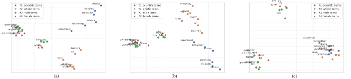
Figure 1: The topology of a vector space before and after debiasing. Terms from WEAT T8 test: $T_{1}$ – science terms (blue), $T_{2}$ – art terms (orange), $A_{1}$ – male terms (green), and $A_{2}$ – female terms (red). 2D projection with PCA. (a) Distributional en FT vectors; (b) Debiased using BAM; (c) Debiased using GBDD.

Biases of Distributional Spaces. The main results are summarized in Table 2. All three input distributional spaces generally exhibit explicit and implicit biases, with CBOW spaces displaying the lowest biases, both according to the WEAT tests (e.g., the effect size is even insignificant with $p<0.05$ for the gender bias test T8) and the implicit bias tests of ? (?). Interestingly – according to our BAT test, and despite the original claims and examples from ? (?) – the encoded biases do not reflect strongly in the analogy tests. Nonetheless, our debiasing methods in most test settings manage to affect the input vector spaces by further reducing BAT scores.

Comparison of Debiasing Models.

While the results vary across the two WEAT tests and evaluation metrics, GBDD emerges as the most robust model on average. It attenuates the explicit bias while being the most successful in removing the bias implicitly: the spaces debiased with GBDD completely confuse the KM clustering and SVM classifier. It also fully retains the useful semantic information: we do not observe drops on SL and WS compared to the input distributional spaces. While GBDD outperforms BAM and DebiasNet (DBN) on average according to ECT and BAT measures, it is not able to fully remove the explicit gender bias (T8) according to the WEAT test.

Despite operating on an implicit specification $B_{I}$, BAM removes the explicit biases much better than the implicit ones. DBN seems even better than BAM in removing the explicit biases. This is not a surprise, since DBN is trained on an explicit bias specification. However both DBN and BAM are unsuccessful in removing the implicit biases. Moreover, DBN distorts the input space more than BAM, yielding substantial drops on SL and WS.

The complementarity of debiasing effects between GBDD, and BAM/DBN are confirmed by the performance of their compositions. All composition models robustly remove both explicit and implicit biases, also showing that there is no “one model rules them all” solution to various debiasing aspects. GBDD $\circ$ DBN most effectively removes the biases, but it inherits the undesirable semantic distortions of DBN. On the other hand, BAM $\circ$ GBDD offers solid bias removal while for the most part retaining the semantic quality of the space.

Differences between Evaluation Measures.

The three aspects of evaluation complement each other: they all inform the selection of the most appropriate debiasing model w.r.t. the desired application-specific criteria. However, results of WEAT, ECT, and BAT are not always aligned. For example, the CBOW space is unbiased according to the WEAT test, but extremely biased (negative correlation!) according to ECT. In contrast, GloVe vectors are biased according to WEAT but not according to ECT (correlation of $0.84$). These findings point to different bias aspects, accentuating the need for multiple, mutually complementary, bias measures.

Cross-Lingual Transfer

The results in the cross-lingual debiasing transfer are shown in Table 3. For brevity, we show only the results on XWEAT T8 (gender bias wrt. science vs. art) and for a subset of evaluation measures (one for each evaluation aspect): WEAT (W), KMeans++ (KM), and SimLex (SL).^,

We first confirm the results from ? (?): de, it, ru, and hr fastText vectors do not exhibit significant explicit gender bias (wrt. science vs. art), according to the WEAT test. The explicit bias is, however, significant in es and tr distributional vectors. Implicit bias is clearly present in all distributional spaces except ru. Debiasing models display similar properties as before: DBN reduces the explicit bias more effectively than BAM and GBDD, but it semantically distorts the vectors; and only GBDD successfully removes the implicit bias. None of the models fully removes the explicit bias for tr (the lowest bias effect of $0.99$ for BAM $\circ$ GBDD is still significant). We suspect that this is a result of the lower-quality cross-lingual tr$\rightarrow$en projection, which is in line with the bilingual lexicon induction results from ? (?).

For de and it, BAM and DBN invert the direction of the bias: negative WEAT scores mean that sciences are more correlated with female attributes and arts with male attributes. We believe that this is the result of applying a (strong) bias correction learned on a biased en space on the (explicitly) unbiased de and it spaces. The BAM $\circ$ GBDD composition seems most robust in the cross-lingual transfer setting – it successfully removes both the explicit (if they exist) and implicit biases, while preserving useful semantic information (SL). These results indicate that we can attenuate or remove biases in distributional vectors of languages for which (1) we do not require the initial bias specification and (2) we do not even need similarity-specialized word embeddings used to augment the bias specifications for the target language.

Topology of Debiased Spaces.

Finally, we qualitatively analyze the debiasing effects suggested by evaluation measures. We project the input and the debiased embeddings into 2D with PCA, and show the constellation of words from the initial bias specification of WEAT T8 (Table 1) in Figure 1. In the distributional space, the two target sets (science vs art) are clearly distinguishable from one another (implicit bias), and so are the male and female attributes. The science terms are notably closer to the male terms and art terms to the female terms (explicit bias). The space produced by BAM intertwines the male and female terms and makes the science and art terms roughly equidistant to the gender terms (explicit bias removed), but the science terms are still clearly distinguishable from art terms (implicit bias still present). In the space produced by GBDD, both biases are removed: science and art terms cannot be clearly separated and are roughly equidistant to gender terms.

Conclusion

We have introduced a general framework for debiasing distributional word vector spaces by 1) formalizing the differences between implicit and explicit biases, 2) proposing new debiasing methods that deal with the two different bias specifications, and 3) designing a comprehensive evaluation framework for testing the (often complementary) effects of debiasing. While the proposed framework offers a systematized view on human biases encoded in word embeddings, the main results indicate that our debiasing methods can effectively attenuate biases in arbitrary input distributional spaces and can also be transferred to a variety of target languages.

		DE							ES
		Explicit			Implicit		SemQ		Explicit			Implicit		SemQ
Model		WEAT	ECT	BAT	KM	SVM	SL	WS	WEAT	ECT	BAT	KM	SVM	SL	WS
WEAT1	Distributional	1.36	41.7	59.9	98.9	75.7	40.7	68.0	1.47	61.8	48.1	100	57.5	–	–
	GBDD	0.42*	77.7	48.2	90.5	51	40.7	68.1	0.56	89.4	34.4	96.8	50.3	–	–
	BAM	1.39	50.6	54	95	94.3	39	64.5	1.12	62.9	42.2	97.7	95.3	–	–
	DN	0.42*	48.1	48.3	98.9	53	39.9	61.9	0.96	55.8	41.6	97.7	34.4	–	–
	GBDD $\circ$ BAM	0.61	81.1	44.3	93.2	88.4	39.1	64.7	0.56	76.4	38.2	98.4	77	–	–
	BAM $\circ$ GBDD	0.75	74.3	52.4	90.8	50	40.8	64.9	0.48*	85.3	42.8	94.1	49.5	–	–
	GBDD $\circ$ DN	0.30*	82.8	45.7	86.6	42.9	39.6	61.9	0.69	75.1	38	96.2	38.3	–	–
WEAT8	Distributional	0.05*	34.1	37.2	98.3	50	40.7	68	1.16	67.8	36.4	99.8	50	–	–
	GBDD	0.15*	85.3	30.5	55.4	50	40.7	67.7	0.41*	70.9	31.1	60	50	–	–
	BAM	-0.97	41.5	33.6	97.4	100	40.7	65.8	0.11*	70.9	34.4	99	100	–	–
	DN	-0.1*	67.1	37.4	97.4	50	36.2	62	0.76*	74	48.1	100	50	–	–
	GBDD $\circ$ BAM	-0.12*	83.2	35.2	56.3	50	40.8	65.6	0.05*	83.7	33.1	58	50	–	–
	BAM $\circ$ GBDD	-0.09*	84.4	28.5	54.4	50	37.3	66.7	0.11*	85.9	28.1	56.6	50	–	–
	GBDD $\circ$ DN	0.35*	73.4	35.7	57.6	50	35.9	61.1	0.78*	88.5	46.4	52.4	50	–	–

Table 4: Complete cross-lingual debiasing transfer results for transfer to German (de) Spanish (es). Results obtained on the XWEAT (?) T1 and T8 tests of respective languages.

		IT							RU
		Explicit			Implicit		SemQ		Explicit			Implicit		SemQ
Model		WEAT	ECT	BAT	KM	SVM	SL	WS	WEAT	ECT	BAT	KM	SVM	SL	WS
WEAT1	Distributional	1.28	57.7	57.2	97	54.8	29.8	64.2	1.28	57.6	43.5	96.7	54.3	25.6	59.2
	GBDD	0.02*	81.8	44	77.3	51.1	29.8	64	0.67	79.8	35.3	93.5	49.9	25.4	59
	BAM	1.35	54	55.5	95.9	95.6	27.3	62.2	1.20	66	44.4	94.4	94.3	24.2	55.5
	DN	0.53	62.8	51.9	99.8	55.5	25.7	58.5	0.44*	57.7	42.7	96.5	56.3	24.3	52.6
	GBDD $\circ$ BAM	0.44*	70.9	51.4	87.7	86.2	27.3	62.2	0.6	80.7	40.1	93.5	89	24.2	55.4
	BAM $\circ$ GBDD	0.29*	76.5	48.6	73.4	50.2	28.2	62.4	0.65	80.2	37.7	92.8	49.6	25	56.3
	GBDD $\circ$ DN	0.2*	83.5	48	88.1	57.6	25.8	58.3	0.36*	75	40.7	91.1	52.4	24.1	52.5
WEAT8	Distributional	0.10*	92.5	25.9	99.8	50	29.8	64.2	0.37*	49.9	32.1	62	50	25.6	59.2
	GBDD	-0.28*	86.4	25.9	56.1	50	29.8	63.4	0.73*	49.5	32	62.4	50	25.8	58.3
	BAM	-0.70*	57.4	23	99.6	100	29	61	-0.41*	44.6	25.9	74.4	100	25.1	56.8
	DN	-1.05	40.7	14.1	100	50	25.4	57.7	0.31*	46.8	35.5	77.9	50	20.7	56.9
	GBDD $\circ$ BAM	-0.62*	67	23.1	57.9	50	29	60	0.34*	72.7	30.8	56.8	50	24.8	55.8
	BAM $\circ$ GBDD	-0.05*	82.3	28.9	58.9	50	27.1	60.2	0.59*	83.7	31	61.6	50	25.4	57.5
	GBDD $\circ$ DN	-0.64*	51.2	18.7	60.1	50	25	56.7	0.77*	69.7	38.3	61.9	50	20.7	55.1

Table 5: Complete cross-lingual debiasing transfer results for transfer to Italian (it) and Russian (ru). Results obtained on the XWEAT (?) T1 and T8 tests of respective languages.

		HR							TR
		Explicit			Implicit		SemQ		Explicit			Implicit		SemQ
Model		WEAT	ECT	BAT	KM	SVM	SL	WS	WEAT	ECT	BAT	KM	SVM	SL	WS
WEAT1	Distributional	1.45	56.3	63.4	57	51.7	32.7	–	1.21	69.6	47.9	86.3	50.6	–	–
	GBDD	0.85	81.2	60.5	63.2	49.8	32.8	–	0.64	83.9	40.9	79.7	51.4	–	–
	BAM	1.35	50.8	63.8	59.5	90.5	31.2	–	0.89	64.8	39.1	84.3	90.6	–	–
	DN	0.86	74.8	67.2	87.4	35.8	28.4	–	0.78	73.3	36.9	88.1	58.3	–	–
	GBDD $\circ$ BAM	0.82	63.6	57.1	55.1	77.5	31.3	–	0.19*	80	34.5	72	73.2	–	–
	BAM $\circ$ GBDD	0.71	86.8	63	68.7	50	30.9	–	0.76	82.3	53	75	51.1	–	–
	GBDD $\circ$ DN	0.56*	85.9	65.5	61.4	44	28.5	–	0.63	81.5	33	74.7	54.9	–	–
WEAT8	Distributional	0.13*	53.2	39.4	98.6	50	32.7	–	1.72	39.6	64.5	99.3	50	–	–
	GBDD	0.54*	59.7	40.2	59.9	50	32.5	–	1.41	71.9	66.5	64.3	50	–	–
	BAM	-0.01*	30.3	41.1	93.5	100	32	–	1.49	62.1	59.5	98.8	100	–	–
	DN	0.25*	81.7	52.8	99.9	50	25.3	–	1.54	44.6	65.5	100	50	–	–
	GBDD $\circ$ BAM	0.52*	73.8	47	60.8	50	31.7	–	0.99	85.3	56	56.9	50	–	–
	BAM $\circ$ GBDD	0.68*	60.9	44.5	75.4	50	29.4	–	1.27	59.3	76	62.4	50	–	–
	GBDD $\circ$ DN	0.67*	88.5	56.6	67.5	50	25.1	–	1.29	86.7	65	62.5	50	–	–

Table 6: Complete cross-lingual debiasing transfer results for transfer to Croatian (hr) and Turkish (tr). Results obtained on the XWEAT (?) T1 and T8 tests of respective languages.

Initial	$T_{1}$	aster clover hyacinth marigold poppy azalea crocus iris orchid rose blue-bell daffodil lilac pansy tulip buttercup daisy lily peony violet carnation gladiola magnolia petunia zinnia
	$T_{2}$	ant caterpillar flea locust spider bedbug centipede fly maggot tarantula bee cockroach gnat mosquito termite beetle cricket hornet moth wasp blackfly dragonfly horsefly roach weevil
	$A_{1}$	caress freedom health love peace cheer friend heaven loyal pleasure diamond gentle honest lucky rainbow diploma gift honor miracle sunrise family happy laughter paradise vacation
	$A_{2}$	abuse crash filth murder sickness accident death grief poison stink assault disaster hatred pollute tragedy divorce jail poverty ugly cancer kill rotten vomit agony prison
k=2	$T_{1}$	glovers gladiolus nance crowfoot meadowsweet dianthus pinkish dolly poppies cyclamen tulips sapphire azaleas wisteria camellia asters trefoil sissy olive penstemon candlewood prunella primula mauve opium buddleja taupe magenta veronica hyacinths magnolias watercress minaj cowslip lilies tulipa orchis daffodils scarlet jasmine faggot marigolds orchids
	$T_{2}$	caterpillars gnats termites avenger ants bumblebee arachnid sticking cricketing flit tarantulas pyralidae harrier millipede centipedes mosquitos vermin worm cockroaches locusts wasps insect snook larva scoot gracillariidae weevils grasshopper undershot fathead whitefly louse batsman dragonflies
	$A_{1}$	donation liberty tranquility fortunate mild laugh diamonds holiday truthful endowment untried fitness colleague credentials lineage gurgling honour faithful cheerfulness auspicious affection prism genuine esteem moonlight newfound vacations gem eden peacefulness gladden wellness partner glad cuddle cherish joy liege diplomas phenomenon fondle autonomy prodigy tickled enjoyment clement utopia tribe
	$A_{2}$	misuse collision stench destitution demise anguish annihilate estrangement illness incarcerate sorrow mistreat infection destroy separation slaughter antipathy penitentiary smash regurgitate malady misery decease dirt calamity impoverishment spew stinking toxin enmity imprison tainted massacre gaol sinister horrible defile contaminate reek prostate catastrophe crud casualty mishap leukemia invasion misadventure onslaught
k=3	$T_{1}$	faggot cornflower meadowsweet cowslip camellia cress weeknd orchidaceae watercress trefoil pinkish magnoliaceae orchids lilies dianthus hyacinths primula willowherb daffodils mauve penstemon azaleas fleabane magenta wisteria jessie licorice lilacs polly peonies magnolias candlewood amaranthus jasmine opium bluish poppies sapphire orchis sissy buddleja tangerine olive clovers marigolds lavender dandelions tulipa taupe tulips poof crowfoot gladiolus prunella dandelion veronica dolly asters cyclamen scarlet minaj nance
	$T_{2}$	projected avenger grasshopper vermin scamper worm cockroaches fathead harrier batsman weevils snook whitefly bug noctuidae scorpion mayfly tarantulas louse roaches cricketing bumblebee gnats curculionidae arachnid mosquitoes wasps dragonflies scoot termites larva millipede corsair flit gracillariidae locusts wicket hive insect caterpillars mosquitos parasitoid undershot sticking centipedes ants pyralidae fleas
	$A_{1}$	fortunate colleague auspicious peacefulness untried jewel propitious cherish joy truthful stunner hug dearest partner comrade honour gladden glad bliss delight encourage mild eden laugh moonlight genuine tickled joyful diamonds gem gratuity sabbatical enjoyment lineage endowment liberty certificate newfound liege wellness gurgling credentials clement utopia autonomy faithful tribe chuckle vacations prism holiday serenity sincere phenomenon diplomas homage rainbows donation cuddle welfare tranquility affection allegiant independency tranquil prodigy esteem fondle cheerfulness ancestry fitness untested
	$A_{2}$	severance reek imprison onslaught surly destroy massacre invasion complaint spew dirt casualty heartbreak slaying stinking catastrophe penitentiary demise slaughter privation toxin illness impoverishment annihilate calamity contaminate separation collision outrage grime stench disgorge mishap collide hate regurgitate crud misuse malady contagion sinister infection smash attack leukemia tumour tainted anguish defile stinky ailment gaol decease extinguish enmity sorrow misadventure expiration pollutes antipathy estrangement misery incarcerate horrible prostate destitution mistreat
k=4	$T_{1}$	scarlet bluebell cornflower delphinium fleabane amaranthus dianthus chromatic poof peonies orchidaceae orchis azaleas mauve tangerine nance tulipa camellia taupe willowherb hyacinths minaj periwinkle helianthemum poppies lilies cress magnolias macklemore dolly sissy sapphire orchids buddleja licorice jasmine faggot tulips lavender opium dandelion weeknd wisteria cowslip prunella thyme alfalfa lilacs daffodils magnoliaceae pinkish watercress crowfoot veronica primula carrie bluish cryptanthus trefoil asters jessie polly olive clovers meadowsweet fuchsia penstemon candlewood marigolds dandelions cyclamen snowberry purplish sassafras gladiolus epiphyte magenta
	$T_{2}$	caterpillars wasps corsair whitefly insect bumblebee bowler noctuidae yellowjacket mayfly curculionidae cockroaches dragonflies avenger mulligan pilotless roundworm undershot protruding grasshopper crambidae damselfly louse projected cricketing vermin parasitoid tarantulas wicket sticking scorpion gnats hellcat mosquitoes sawfly hive arachnid larva locusts centipedes snook batsman weevils dart flit bug fleas gracillariidae harrier burrowing scamper roaches hickory mosquitos scoot tractor fathead worm bumblebees millipede pyralidae termites leafhopper ants
	$A_{1}$	independency rhombus daybreak endowment enliven vacationing cheerful tribe partner privilege truthful rainbows gem gratification gratuity affection phenomenon delight untried daydream mirth fondle tranquility prism gladden enjoyment esteem stunner certificate genuine holiday glad sabbatical encourage autonomy cherish baccalaureate favorable credentials donation tranquil fitness wellness mild reverence hug benefaction gracious diplomas ancestry nirvana staunch chuckle vacations cuddle marvel propitious liege gurgling serenity peacefulness honour kiss allegiant utopia welfare sincere clement jewel eden fortunate faithful joyful prodigy moonlight homage diamonds tickled laugh dearest sidekick colleague untested bliss cheerfulness lineage liberty parentage idolize calmness authentic comrade joy auspicious newfound wellbeing
	$A_{2}$	stinky protest mistreat sorrow disease maltreatment taint remand horrible casualty contaminate smash misery misuse annihilate imprison crud raid grime pollutes contagion barf infection hate decease slaughter destroy calamity sinister breakup expiration enmity carnage hideous demise regurgitate stench tainted outrage stockade dying separation invasion shatter antipathy happening extinguish privation spew tumour ailment complaint attack destitution exterminate rancid massacre impoverishment slaying heartache misfortune incarcerate disgorge surly malady catastrophe onslaught collide misadventure defile gaol prostate dirt penitentiary anguish dearth animosity muck heartbreak reek severance contamination collision estrangement illness leukemia tumor mishap toxin stinking

Table 7: Bias specification of WEAT T1: sentiment attached to flowers ($T_{1}$) vs. insects ($T_{2}$). Original terms from ? (?) and augmented list for different $k$.

Initial	$T_{1}$	science technology physics chemistry Einstein NASA experiment astronomy
	$T_{2}$	poetry art Shakespeare dance literature novel symphony drama
	$A_{1}$	brother father uncle grandfather son he his him
	$A_{2}$	sister mother aunt grandmother daughter she hers her
k=2	$T_{1}$	automation radiochemistry test biophysics learning electrodynamics biochemistry astrophysics erudition astrometry technologies experimentation
	$T_{2}$	orchestra artistry dramaturgy poesy philharmonic craft untried hop poem dancing dissertation treatise new dramatics
	$A_{1}$	beget buddy forefather man nephew own himself theirs boy helium crony cousin grandpa granddad herself
	$A_{2}$	niece girl parent grandma granny woman theirs sire auntie sibling herself jealously stepmother wife
k=3	$T_{1}$	technologies biochemistry astrophysics engineering electrodynamics radiochemistry astronomer erudition education automation biophysics chromodynamics research learning experimentation test astrometry biology
	$T_{2}$	groundbreaking craftsmanship dissertation new literatures dramatization philharmonic sinfonietta artistry untried poems dramaturgy dancing dramatics poem poesy craft hop treatise orchestra waltz
	$A_{1}$	granddad granddaddy man helium grandpa own himself forefather themself kinsman theirs sire beget boy buddy herself comrade who crony nephew grandson cousin
	$A_{2}$	sire beget stepmother aunty parent woman grandma herself own stepsister female girl jealously sibling auntie theirs granny niece wife
k=4	$T_{1}$	physicists test electrochemistry automation engineering biophysics education learning chromodynamics technologies radiochemistry examination biology technological astronomer astrophysics experimentation biochemistry research lore electrodynamics astrobiology astrometry erudition
	$T_{2}$	dramaturgy monograph untried dances poesy dissertation craftsmanship orchestra treatise skill waltz poem literatures dramatization poems theatre dancing newfound hop artistry new verse craft philharmonic concerto groundbreaking dramatics sinfonietta
	$A_{1}$	grandad theirs grandson buddy themself stepbrother forefather ironically crony granddaddy grandpa sidekick boy heir granddad cousin who male man sire parent beget kinsman nephew herself own comrade himself helium
	$A_{2}$	auntie fiance theirs female stepmother grandma woman procreate stepsister widow aunty grandmothers mimi granny sibling wife sire parent beget niece herself own girl jealously siblings
k=5	$T_{1}$	experimentation lore research chromodynamics astrobiology technological technologies physicists education investigation engineering examination radiochemistry biology astrophysics astrology chemistries learning biochemistry electrochemistry biophysics astronomer test scholarship electrodynamics biotechnology erudition automation astrometry
	$T_{2}$	new untried literatures rhyme sinfonietta monograph philharmonic hop expertise craft dancing theater dances newfound artistry dramatics untested writing orchestra dramatization poesy craftsmanship dramaturgy jitterbug theatre treatise concerto poem orchestral verse poems waltz dissertation groundbreaking skill
	$A_{1}$	granddad crony its granddaddy male helium herself forefather heir granduncle own sidekick grandson comrade grandfathers sire nephew man stepbrother grandad theirs cousin who hesitates themself parent grandpa kinsman ironically himself boy buddy spawn beget
	$A_{2}$	female wife kinswoman girl herself stepsisters stepsister grandmothers own granny stepmother affections woman sire spouse lady theirs fiance aunty procreate progenitor parent jealously sisters siblings niece widow mimi auntie matriarch sibling grandma beget

Table 8: Bias specification of WEAT T8: female vs. male attributes attached to science ($T_{1}$) vs. art ($T_{2}$). Original terms from ? (?) and augmented list for different $k$.

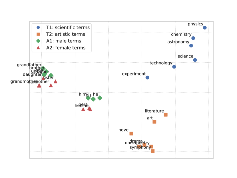
Figure 2: The topology of a vector space before debiasing. Terms from WEAT T8 test: $T_{1}$ – science terms (blue), $T_{2}$ – art terms (orange), $A_{1}$ – male terms (green), and $A_{2}$ – female terms (red). 2D projection with PCA.

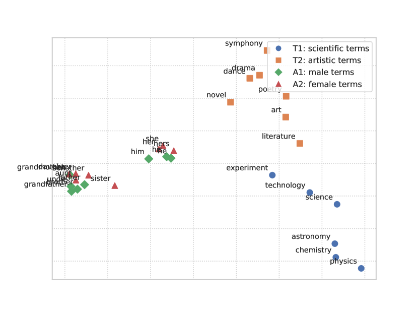
Figure 3: The topology of a vector space after debiasing. Terms from WEAT T8 test: $T_{1}$ – science terms (blue), $T_{2}$ – art terms (orange), $A_{1}$ – male terms (green), and $A_{2}$ – female terms (red). 2D projection with PCA. Debiased using BAM.

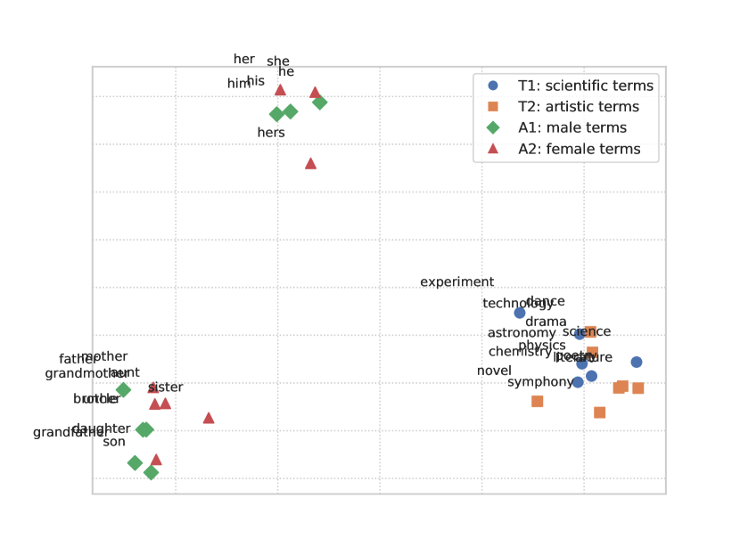
Figure 4: The topology of a vector space after debiasing. Terms from WEAT T8 test: $T_{1}$ – science terms (blue), $T_{2}$ – art terms (orange), $A_{1}$ – male terms (green), and $A_{2}$ – female terms (red). 2D projection with PCA. Debiased using GBDD.

Figure 5: The topology of a vector space after debiasing. Terms from WEAT T8 test: $T_{1}$ – science terms (blue), $T_{2}$ – art terms (orange), $A_{1}$ – male terms (green), and $A_{2}$ – female terms (red). 2D projection with PCA. Debiased using DN.

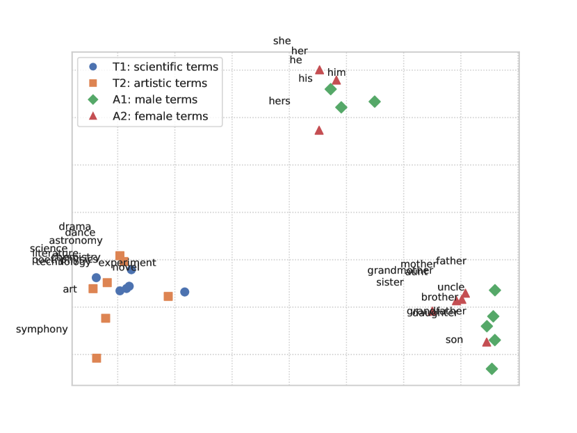
Figure 6: The topology of a vector space after debiasing. Terms from WEAT T8 test: $T_{1}$ – science terms (blue), $T_{2}$ – art terms (orange), $A_{1}$ – male terms (green), and $A_{2}$ – female terms (red). 2D projection with PCA. Debiased using GBDD $\circ$ BAM .

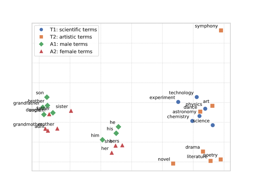
Figure 7: The topology of a vector space after debiasing. Terms from WEAT T8 test: $T_{1}$ – science terms (blue), $T_{2}$ – art terms (orange), $A_{1}$ – male terms (green), and $A_{2}$ – female terms (red). 2D projection with PCA. Debiased using BAM $\circ$ GBDD .

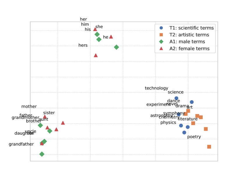
Figure 8: The topology of a vector space after debiasing. Terms from WEAT T8 test: $T_{1}$ – science terms (blue), $T_{2}$ – art terms (orange), $A_{1}$ – male terms (green), and $A_{2}$ – female terms (red). 2D projection with PCA. Debiased using GBDD $\circ$ DN.

References

- [2018] Artetxe, M.; Labaka, G.; and Agirre, E. 2018. A robust self-learning method for fully unsupervised cross-lingual mappings of word embeddings. In Proceedings of ACL, 789–798.
- [2017] Bojanowski, P.; Grave, E.; Joulin, A.; and Mikolov, T. 2017. Enriching word vectors with subword information. Transactions of the ACL 5:135–146.
- [2016] Bolukbasi, T.; Chang, K.-W.; Zou, J.; Saligrama, V.; and Kalai, A. 2016. Man is to computer programmer as woman is to homemaker? Debiasing word embeddings. In Proceedings of NIPS, 4356–4364.
- [2017] Caliskan, A.; Bryson, J. J.; and Narayanan, A. 2017. Semantics derived automatically from language corpora contain human-like biases. Science 356(6334):183–186.
- [2018] Conneau, A.; Lample, G.; Ranzato, M.; Denoyer, L.; and Jégou, H. 2018. Word translation without parallel data. In Proceedings of ICLR.
- [2019] Dev, S., and Phillips, J. 2019. Attenuating bias in word vectors. In Proceedings of AISTATS.
- [2015] Faruqui, M.; Dodge, J.; Jauhar, S. K.; Dyer, C.; Hovy, E.; and Smith, N. A. 2015. Retrofitting word vectors to semantic lexicons. In Proceedings of NAACL-HLT, 1606–1615.
- [2002] Finkelstein, L.; Gabrilovich, E.; Matias, Y.; Rivlin, E.; Solan, Z.; Wolfman, G.; and Ruppin, E. 2002. Placing search in context: The concept revisited. ACM Transactions on information systems 20(1):116–131.
- [2018] Garg, N.; Schiebinger, L.; Jurafsky, D.; and Zou, J. 2018. Word embeddings quantify 100 years of gender and ethnic stereotypes. PNAS 115(16):3635–3644.
- [2018] Glavaš, G., and Vulić, I. 2018. Explicit retrofitting of distributional word vectors. In Proceedings of ACL, 34–45.
- [2019] Glavaš, G.; Litschko, R.; Ruder, S.; and Vulić, I. 2019. How to (properly) evaluate cross-lingual word embeddings: On strong baselines, comparative analyses, and some misconceptions. In Proceedings of ACL, 710–721.
- [2019] Gonen, H., and Goldberg, Y. 2019. Lipstick on a pig: Debiasing methods cover up systematic gender biases in word embeddings but do not remove them. In Proceedings of NAACL-HLT, 609–614.
- [1954] Harris, Z. S. 1954. Distributional structure. Word 10(23):146–162.
- [2015] Hill, F.; Reichart, R.; and Korhonen, A. 2015. Simlex-999: Evaluating semantic models with (genuine) similarity estimation. Computational Linguistics 41(4):665–695.
- [2019] Lauscher, A., and Glavaš, G. 2019. Are we consistently biased? Multidimensional analysis of biases in distributional word vectors. In Proceedings of *SEM, 85–91.
- [2015] Leviant, I., and Reichart, R. 2015. Separated by an un-common language: Towards judgment language informed vector space modeling. arXiv preprint arXiv:1508.00106.
- [2019] Manzini, T.; Chong, L. Y.; Black, A. W.; and Tsvetkov, Y. 2019. Black is to criminal as caucasian is to police: Detecting and removing multiclass bias in word embeddings. In Proceedings of NAACL-HLT, 615–621.
- [2013] Mikolov, T.; Sutskever, I.; Chen, K.; Corrado, G. S.; and Dean, J. 2013. Distributed representations of words and phrases and their compositionality. In Proceedings of NeurIPS, 3111–3119.
- [1995] Miller, G. A. 1995. WordNet: A lexical database for English. Communications of the ACM 38(11):39–41.
- [2017] Mrkšić, N.; Vulić, I.; Ó Séaghdha, D.; Leviant, I.; Reichart, R.; Gašić, M.; Korhonen, A.; and Young, S. 2017. Semantic specialisation of distributional word vector spaces using monolingual and cross-lingual constraints. Transactions of the ACL 5:309–324.
- [2018] Park, J. H.; Shin, J.; and Fung, P. 2018. Reducing gender bias in abusive language detection. In Proceedings of EMNLP, 2799–2804.
- [2014] Pennington, J.; Socher, R.; and Manning, C. 2014. Glove: Global vectors for word representation. In Proceedings of EMNLP, 1532–1543.
- [2018] Peters, M.; Neumann, M.; Iyyer, M.; Gardner, M.; Clark, C.; Lee, K.; and Zettlemoyer, L. 2018. Deep contextualized word representations. In Proceedings of NAACL-HLT, 2227–2237.
- [2018] Ponti, E. M.; Vulić, I.; Glavaš, G.; Mrkšić, N.; and Korhonen, A. 2018. Adversarial propagation and zero-shot cross-lingual transfer of word vector specialization. In Proceedings of EMNLP, 282–293.
- [2019] Ruder, S.; Vulić, I.; and Søgaard, A. 2019. A survey of cross-lingual word embedding models. Journal of Artificial Intelligence Research 65:569–631.
- [2018] Rudinger, R.; Naradowsky, J.; Leonard, B.; and Van Durme, B. 2018. Gender bias in coreference resolution. In Proceedings of NAACL-HLT, 8–14.
- [1966] Schönemann, P. H. 1966. A generalized solution of the orthogonal Procrustes problem. Psychometrika 31(1):1–10.
- [2017] Smith, S. L.; Turban, D. H.; Hamblin, S.; and Hammerla, N. Y. 2017. Offline bilingual word vectors, orthogonal transformations and the inverted softmax. In Proceedings of ICLR.
- [2018] Vulić, I.; Glavaš, G.; Mrkšić, N.; and Korhonen, A. 2018. Post-specialisation: Retrofitting vectors of words unseen in lexical resources. In Proceedings of the NAACL-HLT, 516–527. New Orleans, Louisiana: Association for Computational Linguistics.
- [2017] Zhao, J.; Wang, T.; Yatskar, M.; Ordonez, V.; and Chang, K.-W. 2017. Men also like shopping: Reducing gender bias amplification using corpus-level constraints. In Proceedings of EMNLP, 2979–2989.
- [2018a] Zhao, J.; Wang, T.; Yatskar, M.; Ordonez, V.; and Chang, K.-W. 2018a. Gender bias in coreference resolution: Evaluation and debiasing methods. In Proceedings of NAACL-HLT, 15–20.
- [2018b] Zhao, J.; Zhou, Y.; Li, Z.; Wang, W.; and Chang, K.-W. 2018b. Learning gender-neutral word embeddings. In Proceedings of EMNLP, 4847–4853.
- [2019] Zhao, J.; Wang, T.; Yatskar, M.; Cotterell, R.; Ordonez, V.; and Chang, K.-W. 2019. Gender bias in contextualized word embeddings. In Proceedings of NAACL-HLT, 629–634.