Orlicz-space regularization for optimal transport and algorithms for quadratic regularization

Abstract

We investigate the continuous optimal transport problem in the so-called Kantorovich form, i.e. given two Radon measures on two compact sets, we seek an optimal transport plan which is another Radon measure on the product of the sets that has these two measures as marginals and minimizes a certain cost function. We consider regularization of the problem with so-called Young’s functions, which forces the optimal transport plan to be a function in the corresponding Orlicz space rather than a Radon measure. We derive the predual problem and show strong duality and existence of primal solutions to the regularized problem. Existence of (pre-)dual solutions will be shown for the special case of $L^{p}$ regularization for $p\geq 2$. Then we derive four algorithms to solve the dual problem of the quadratically regularized problem: A cyclic projection method, a dual gradient decent, a simple fixed point method, and Nesterov’s accelerated gradient, all of which have a very low cost per iteration.

1 Introduction

We consider the optimal transport problem in the following form: For compact sets $\Omega_{1},\,\Omega_{2}\subset\mathbb{R}^{n}$, measures $\mu_{1},\mu_{2}$ on $\Omega_{1},\Omega_{2}$, respectively, with the same total mass and a real-valued cost function $c:\Omega_{1}\times\Omega_{2}\to\mathbb{R}$ we want to solve

$$\inf_{\pi}\int_{\Omega_{1}\times\Omega_{2}}c\,{\mathrm{d}}\pi$$

where the infimum is taken over all measures on $\Omega_{1}\times\Omega_{2}$ which have $\mu_{1}$ and $\mu_{2}$ as their first and second marginals, respectively (see [16, 23]). Since optimal plans $\pi$ tend to be singular measures (even for marginals with smooth densities [24, 20]), regularization of the problem have become more important, most prominently entropic regularization [7, 10, 3, 11, 9] which ensures that optimal plans have densities. It has been shown in [9] that the analysis of entropically regularized optimal transport problems naturally takes place in the function space $L\log L$ (also called Zygmund space[4]) and that optimal plans for entropic regularization are always in $L\log L(\Omega_{1}\times\Omega_{2})$ and exist if and only if the marginals are in the spaces $L\log L(\Omega_{i})$. These spaces are an example of so-called Orlicz spaces [17] and hence, we consider regularization in these spaces in this paper. Another motivation to study a more general regularization comes from the fact that regularization with the $L^{2}$-norm have been shown to be beneficial in some applications, see [18, 5, 12, 15].

To simplify notation, denote $\Omega:=\Omega_{1}\times\Omega_{2}$. The regularized problems we consider are

$$\inf_{\begin{subarray}{c}\pi\geq 0,\\ (P_{i})_{\#}{\pi}={\mu_{i}},\,i=1,2\end{subarray}}\int_{\Omega}c\,{\mathrm{d}}\pi+\gamma\int_{\Omega}\Phi\circ\pi\,\mathrm{,}$$ (P)

where $\gamma>0$ and the infimum is taken over all positive measure, which have densities with respect to the Lebesgue measure and the constraints $(P_{i})_{\#}{\pi}={\mu_{i}}$ state that $\pi$ should have the marginals $\mu_{i}$. The two main cases we will consider in this paper are $\Phi(t)=t\log t$ (entropic regualarization) and $\Phi(t)=\nicefrac{{t^{2}}}{{2}}$ (quadratic regularization), however, many results in this paper hold for more general functions $\Phi$.

The rest of the paper is organized as follows. First, we introduce the so-called Young’s functions and Orlicz spaces in Section 2. Moreover, a slight generalization of Young’s functions is defined. In Section 3 we give a strong duality result for (P), which allows us to prove existence of primal solutions. Existence of solutions for the (pre-)dual problem will be discussed for the special case $\Phi(t)=\nicefrac{{(t_{+})^{p}}}{{p}}$ for $p\geq 2$. Due to limited space, we omit some proofs in this section and the proofs will be published in an extended version. Finally, we consider numerical methods for the quadratic regularization in Section 4. Here, we will work with the duality result presented in Section 3 and concentrate on algorithms with very low cost per iteration.

2 Young’s Functions & Orlicz Spaces

We briefly introduce some notions about Young’s functions and Orlicz spaces. For a more detailed introduction, see [4, 17].

Definition 2.1 (Young’s function [4, Definition IV.8.1], [8, Eq. (2.22)] ).

1. Let $\phi:[0,\infty)\to{}[0,\infty]$ be increasing and lower semicontinuous, with $\phi(0)=0$. Suppose that $\phi$ is neither identically zero nor identically infinite on $(0,\infty)$. Then the function $\Phi$, defined by

   $$\Phi(t):=\int_{0}^{t}\phi(s)\,{\mathrm{d}}s\,\mathrm{,}$$

   is said to be a Young’s function.

2. A Young’s function $\Phi$ is said to have the $\Delta_{2}$-property near infinity if $\Phi(t)<\infty$ for all $t$ and

   $$\exists C>0,\,t_{0}\geq 0:\,\forall t\geq t_{0}:\,\Phi(2t)\leq C\Phi(t).$$

By definition, Young’s functions are convex and for a Young’s function $\Phi$ it holds that the complementary Young’s function $\Psi(x):=\int_{0}^{x}(\Phi^{\prime})^{-1}(s)\,{\mathrm{d}}s$ is also a Young’s function. Indeed, the complementary Young’s function is related to the convex conjugate $\Phi^{*}$.

The negative entropy regularization uses the regularization functional $\int_{\Omega}\pi\log\pi$ and the function $t\mapsto t\log t$ is not a Young’s function. Hence, we introduce a slight generalization.

Definition 2.2 (Quasi-Young’s functions).

Let $\Phi$ be a Young’s function and $t_{0}\geq 0$. Let $\check{\Phi}$ be a convex, lower semicontinuous function bounded from below with

$$\check{\Phi}(t)=\Phi(t)-\Phi(t_{0})\qquad\forall t\geq t_{0}$$

and $\check{\Phi}(t)\leq 0$ for all $t<t_{0}$. Then $\check{\Phi}$ is said to be a quasi-Young’s function induced by $\Phi$.

Example 2.3.

The function $\check{\Phi}(t)=t\log_{+}t$ is a quasi-Young’s function induced by the Young’s function $\Phi(t)=t\log t$, with $t_{0}=1$. It holds $\Phi(t)=\max\{0,\check{\Phi}(t)\}$.

Definition 2.4 (Orlicz spaces [4, Definition IV.8.10] ).

Let $\Phi$ be a Young’s function and $\Omega\subset\mathbb{R}^{n}$. Define the Luxemburg norm of a measurable function $f:\Omega\to\mathbb{R}$ as

$$\|{f}\|_{{L}^{\Phi}}:=\inf\left\{\gamma\geq 0\>\middle|\>\int_{\Omega}\Phi\circ\left\{\frac{\left|{f}\right|}{\gamma}\right\}\,{\mathrm{d}}\lambda\leq 1\right\}\,\mathrm{.}$$

Then the space

$${L}^{\Phi}(\Omega):=\left\{f:\Omega\to\mathbb{R}\,\text{measurable}\>\middle|\>\|{f}\|_{{L}^{\Phi}}<\infty\right\}$$

of measurable functions on $\Omega$ with finite Luxemburg norm is called the Orlicz space of $\Phi$.

One can verify that the definitions of $\|{\,\boldsymbol{.}\,}\|_{{L}^{\Phi}}$ and ${L}^{\Phi}$ are essentially independent of whether $\Phi$ is a Young’s function or just a quasi-Young’s function. To simplify notation, $\|{\,\boldsymbol{.}\,}\|_{{L}^{\tilde{\Phi}}}$ and ${L}^{\tilde{\Phi}}$ will therefore also be used for quasi-Young’s functions $\tilde{\Phi}$. Note that for a quasi-Young’s function $\tilde{\Phi}$ induced by a Young’s function $\Phi$, it holds that ${L}^{\tilde{\Phi}}={L}^{\Phi}$, while in general $\|{\,\boldsymbol{.}\,}\|_{{L}^{\tilde{\Phi}}}$ and $\|{\,\boldsymbol{.}\,}\|_{{L}^{\Phi}}$ are equivalent but not equal.

It is well known that for a quasi-Young’s function $\Phi$ with $\lim_{t\to\infty}\nicefrac{{\Phi(t)}}{{t}}=\infty$ and bounded domain $\Omega$ it holds that ${L}^{\Phi}(\Omega)\subset{L}^{1}(\Omega)$. Moreover for complementary Young’s functions $\Phi$ and $\Psi$ which are proper, locally integrable and have the $\Delta_{2}$-property near infinity it holds that $({L}^{\Phi}{})^{*}$ is canonically isometrically isomorphic to $({L}^{\Psi},\|{\,\boldsymbol{.}\,}\|_{{L}^{\Psi}})$ (see, e.g. [13]).

Example 2.5 ($L\log L{}$ and $L_{\exp}{}$).

Let $\Phi(t)=t\log t$ and $\tilde{\Phi}(t)=t\log_{+}t$. The space of measurable functions $f$ with $\int_{\Omega}\tilde{\Phi}\circ\left|{f}\right|\,{\mathrm{d}}\lambda<\infty$ is called $L\log L{}$. Because ${L}^{\Phi}={L}^{\tilde{\Phi}}$, the space of measurable functions $g$ with $\int_{\Omega}{\Phi}\circ\left|{g}\right|\,{\mathrm{d}}\lambda<\infty$ is equal to $L\log L$ as well. The complementary Young’s function $\tilde{\Psi}$ of $\tilde{\Phi}$ is given by

$$\tilde{\Psi}(t)=\begin{cases}t,&t\leq 1\\ \mathrm{e}^{t-1},&\text{else.}\end{cases}$$

Hence, the dual space of $L\log L{}$ is given by the space of measurable functions $h$ that satisfy $\int_{\Omega}\tilde{\Psi}\circ\left|{h}\right|\,{\mathrm{d}}\lambda<\infty$, which is called $L_{\exp}{}$.

Similar to [9, Lemma 2.11] one can show that the marginals of a transport plan $\pi\in{L}^{\Phi}$ are also in ${L}^{\Phi}$:

Lemma 2.6.

If $\pi\in{L}^{\Phi}(\Omega)$ for a quasi-Young’s function $\Phi$, then $(P_{i})_{\#}\pi\in{L}^{\Phi}(\Omega_{i})$ for $i=1,2$ with

$$\|{(P_{i})_{\#}\pi}\|_{{L}^{\Phi}}\leq\max\left\{1,\left|{\Omega_{3-i}}\right|\right\}\|{\pi}\|_{{L}^{\Phi}}\,\mathrm{.}$$

Conversely, for the direct product of two marginals to lie in ${L}^{\Phi}(\Omega)$, some assumptions have to be made.

Proposition 2.7.

Let $\Omega_{1},\Omega_{2}\subset\mathbb{R}^{n}$ be bounded and $\Phi$ be a quasi-Young’s function satisfying either

$$\Phi(xy)\leq C\Phi(x)\Phi(y)$$ (2.1)

for some $C>0$ or

$$\begin{split}\Phi(xy)&\leq C_{1}x\Phi(y)+C_{2}\Phi(x)y\\ \frac{\Phi(t)}{t}&\xrightarrow[t\to\infty]{}\infty\end{split}$$ (2.2)

for some $C_{1},C_{2}\geq 0$. If $\pi=\mu_{1}\otimes\mu_{2}$ and $\mu_{i}\in{L}^{\Phi}(\Omega_{i})$ for $i=1,2$, where $(\mu_{1}\otimes\mu_{2})(x_{1},x_{2}):=\mu_{1}(x_{1})\mu_{2}(x_{2})$, then $\pi\in{L}^{\Phi}(\Omega)$.

Example 2.8.

1. For $\Phi(t)=\frac{t^{p}}{p}$, $p>1$, Eqs. 2.2 and 2.1 both hold trivially.

2. For $\Phi(t)=t\log t$, Eq. 2.2 holds, since $\log(xy)=\log(x)+\log(y)$.

3 Existence of Solutions

In this section, strong duality will be shown for the regularized mass transport (P) using Fenchel duality in the spaces ${\mathcal{M}}(\Omega)$ and ${\mathcal{C}}(\Omega)$. Here, the general framework as outlined in e.g.[1, Chap. 9] or [14, Sec. III.4], is used. The result will then be used to study the question of existence of solutions for both the primal and the dual problem.

Theorem 3.1 (Strong duality).

Let $\Phi$ be a quasi-Young’s function and let

$$\tilde{\Phi}(t):=\begin{cases}\infty,&t<0,\\ \Phi(t),&\text{else}.\end{cases}$$

If $\tilde{\Phi}^{*}\circ\left\{\nicefrac{{-c}}{{\gamma}}\right\}$ is integrable, then the predual problem to (P) is

$$\sup_{\begin{subarray}{c}\alpha_{i}\in{\mathcal{C}}(\Omega_{i}),\\ i=1,2\end{subarray}}\int_{\Omega_{1}}\alpha_{1}\,{\mathrm{d}}\mu_{1}+\int_{\Omega_{2}}\alpha_{2}\,{\mathrm{d}}\mu_{2}-\gamma\int_{\Omega}\tilde{\Phi}^{*}\circ\left\{\frac{{\alpha_{1}}\oplus{\alpha_{2}}-c}{\gamma}\right\}\,{\mathrm{d}}\lambda\,,$$ (P*)

where $(\alpha_{1}\oplus\alpha_{2})(x_{1},x_{2}):=\alpha_{1}(x_{1})+\alpha_{2}(x_{2})$, and strong duality holds. Furthermore, if the supremum is finite, (P) posseses a minimizer.

Proof.

This proof follows the outline of the proof in [9, Theorem 3.1]. First note that ${\mathcal{M}}(\Omega)$ is the dual space of ${\mathcal{C}}(\Omega)$ for compact $\Omega$. Furthermore Slater’s condition is fulfilled with ${\alpha_{1}},{\alpha_{2}}=0$ so that strong duality holds and (assuming a finiteness of the supremum) the primal (P) possesses a minimizer. Additionally, the integrand of the last integral in (P*) is normal, so that it can be conjugated pointwise [19, Theorem 2].

Carrying out the conjugation one obtains

$$\sup_{\begin{subarray}{c}\alpha_{i}\in{\mathcal{C}}(\Omega_{i}),\\ i=1,2\end{subarray}} \int_{\Omega_{1}}{\alpha_{1}}\,{\mathrm{d}}\mu_{1}+\int_{\Omega_{2}}{\alpha_{2}}\,{\mathrm{d}}\mu_{2}-\gamma\int_{\Omega}\tilde{\Phi}^{*}\circ\left\{\frac{\alpha_{1}\oplus\alpha_{2}-c}{\gamma}\right\}\,{\mathrm{d}}\lambda$$

$$\begin{multlined}=\sup_{\begin{subarray}{c}\alpha_{i}\in{\mathcal{C}}(\Omega_{i}),\\ i=1,2\end{subarray}}\int_{\Omega_{1}}{\alpha_{1}}\,{\mathrm{d}}\mu_{1}+\int_{\Omega_{2}}{\alpha_{2}}\,{\mathrm{d}}\mu_{2}+\int_{\Omega}\left\{\inf_{\pi}\left\{c-\alpha_{1}\oplus\alpha_{2}\right\}\pi+\gamma\tilde{\Phi}\circ\pi\right\}\,{\mathrm{d}}\lambda\end{multlined}=\sup_{\begin{subarray}{c}\alpha_{i}\in{\mathcal{C}}(\Omega_{i}),\\ i=1,2\end{subarray}}\int_{\Omega_{1}}{\alpha_{1}}\,{\mathrm{d}}\mu_{1}+\int_{\Omega_{2}}{\alpha_{2}}\,{\mathrm{d}}\mu_{2}+\int_{\Omega}\left\{\inf_{\pi}\left\{c-\alpha_{1}\oplus\alpha_{2}\right\}\pi+\gamma\tilde{\Phi}\circ\pi\right\}\,{\mathrm{d}}\lambda$$

$$\begin{multlined}=\sup_{\begin{subarray}{c}\alpha_{i}\in{\mathcal{C}}(\Omega_{i}),\\ i=1,2\end{subarray}}\inf_{\pi}\int_{\Omega}c\pi+\gamma\tilde{\Phi}\circ\pi\,{\mathrm{d}}\lambda+\int_{\Omega_{1}}{\alpha_{1}}\,{\mathrm{d}}({\mu_{1}}-(P_{1})_{\#}\pi)\\ +\int_{\Omega_{2}}{\alpha_{2}}\,{\mathrm{d}}({\mu_{2}}-(P_{2})_{\#}\pi)\end{multlined}=\sup_{\begin{subarray}{c}\alpha_{i}\in{\mathcal{C}}(\Omega_{i}),\\ i=1,2\end{subarray}}\inf_{\pi}\int_{\Omega}c\pi+\gamma\tilde{\Phi}\circ\pi\,{\mathrm{d}}\lambda+\int_{\Omega_{1}}{\alpha_{1}}\,{\mathrm{d}}({\mu_{1}}-(P_{1})_{\#}\pi)\\ +\int_{\Omega_{2}}{\alpha_{2}}\,{\mathrm{d}}({\mu_{2}}-(P_{2})_{\#}\pi)$$

$$=\inf_{\begin{subarray}{c}\pi,\\ (P_{i})_{\#}{\pi}={\mu_{i}},\,i=1,2\end{subarray}}\int_{\Omega}c\,{\mathrm{d}}\pi+\gamma\int_{\Omega}\tilde{\Phi}\circ\pi\,{\mathrm{d}}\lambda$$

$$=\inf_{\begin{subarray}{c}0\leq\pi,\\ (P_{i})_{\#}{\pi}={\mu_{i}},\,i=1,2\end{subarray}}\int_{\Omega}c\,{\mathrm{d}}\pi+\gamma\int_{\Omega}\Phi(\pi)\,{\mathrm{d}}\lambda\,\mathrm{,}$$

which is (P). ∎

Example 3.2.

1. Using $\Phi(t)=t\log t$, one obtaines the result for $L\log L{}$ as stated in [9, Theorem 3.1]

2. Using $\Phi(t)=\nicefrac{{t^{2}}}{{2}}$, one obtains the result for ${L}^{2}$ as stated in [15].

Remark 3.3.

Theorem 3.1 does not claim that the supremum is attained, i.e. the predual problem (P*) admits a solution. Moreover, the solutions of (P*) cannot be unique since one can add and subtract constants to $\alpha_{1}$ and $\alpha_{2}$, respectively, without changing the functional value.

3.1 Existence Result for the Primal Problem

The duality result can now be used to address the question of existence of a solution to (P).

Theorem 3.4.

Problem (P) admits a minimizer $\bar{\pi}$ if and only if $\mu_{i}\in{L}^{\Phi}(\Omega_{i})$ for $i=1,2$ and

$$\mu_{1}\otimes\mu_{2}\in{L}^{\Phi}(\Omega)\quad\forall\mu_{i}\in{L}^{\Phi}(\Omega_{i}),\,i=1,2\,\mathrm{.}$$ (3.1)

In this case, $\bar{\pi}\in{L}^{\Phi}(\Omega)$. Moreover, the minimizer is unique, if $\Phi$ is strictly convex.

Proof.

The proof given in [9, Theorem 3.3] for $\Phi(t)=t\log t$ holds for arbitrary $\Phi$. That is, the necessity of the condition $\mu_{i}\in{L}^{\Phi}(\Omega_{i})$, $i=1,2$ only relies on Lemma 2.6. For sufficiency, it is noted that for $\mu_{i}\in{L}^{\Phi}(\Omega_{i})$, $i=1,2$ it holds that $\pi=\mu_{1}\otimes\mu_{2}\in{L}^{\Phi}(\Omega)$, which is ensured by Eq. 3.1. Thus, the infimum in (P) is finite and weak duality shows that the supremum in (P*) is finite as well. Existence of a solution for (P) now follows from Theorem 3.1.

If strict convexity holds for $\Phi$, it directly implies uniqueness. ∎

Remark 3.5.

For example, Eq. 3.1 is satisfied when $\Phi$ satisfies either Eq. 2.1 or Eq. 2.2 since in those cases Proposition 2.7 holds.

3.2 Existence Result for the Predual Problem

The question of existence of solutions to the predual problem (P*) proves to be more difficult for general Young’s functions. There are results that shows existence for the predual problem in the entropic case [9] and in the quadratic case [15], but their proofs are quite different in nature. Here, we only treat Young’s functions of the type $\Phi(t)=\nicefrac{{t^{p}}}{{p}}$ for $p>1$, i.e, only regularization in $L^{p}$. Note that in this case ${\Phi}^{*}(t)=\nicefrac{{({t}_{+})^{q}}}{{q}}$, where $\nicefrac{{1}}{{p}}+\nicefrac{{1}}{{q}}=1$ and the predual is actually the dual.

Assumption 3.6.

Let $\Omega_{1}$ and $\Omega_{2}$ to be compact comains, let the cost function $c$ be continuous and fulfill $c\geq c^{\dagger}>-\infty$. Furthermore, the marginals ${\mu_{i}}\in{L}^{p}(\Omega_{i})$ satisfy ${\mu_{i}}\geq\delta>0$ a.e. for $i=1,2$ and finally assume that $\int_{\Omega_{1}}{\mu_{1}}=\int_{\Omega_{2}}{\mu_{2}}=1$.

It can not be expected for (P*) to have continuous solutions ${\alpha_{1}}$, ${\alpha_{2}}$. However, observe that the objective function of (P*) is also well defined for functions ${\alpha_{i}}\in{L}^{1}(\Omega_{i})$, $i=1,2$, with ${({\alpha_{1}}\oplus{\alpha_{2}}-c)}_{+}/\gamma\in{L}^{q}(\Omega)$. This gives rise to the following variant of the dual problem, for which existence of minimizers can be shown:

$$\begin{multlined}\min\left\{\Lambda({\alpha_{1}},{\alpha_{2}}):=\frac{1}{q}\|{{({\alpha_{1}}\oplus{\alpha_{2}}-c)}_{+}}\|_{q}^{q}\vspace*{-1em}-\gamma^{q-1}\int_{\Omega_{1}}{\alpha_{1}}\,{\mathrm{d}}\mu_{1}-\gamma^{q-1}\int_{\Omega_{2}}{\alpha_{2}}\,{\mathrm{d}}\mu_{2}\right.\\ \left.\vphantom{\int_{\Omega_{2}}{\alpha_{2}}}\middle|\,\alpha_{i}\in{L}^{1}(\Omega_{i}),\,i=1,2,\,{({\alpha_{1}}\oplus{\alpha_{2}}-c)}_{+}/\gamma\in{L}^{q}(\Omega)\right\}\end{multlined}\min\left\{\Lambda({\alpha_{1}},{\alpha_{2}}):=\frac{1}{q}\|{{({\alpha_{1}}\oplus{\alpha_{2}}-c)}_{+}}\|_{q}^{q}\vspace*{-1em}-\gamma^{q-1}\int_{\Omega_{1}}{\alpha_{1}}\,{\mathrm{d}}\mu_{1}-\gamma^{q-1}\int_{\Omega_{2}}{\alpha_{2}}\,{\mathrm{d}}\mu_{2}\right.\\ \left.\vphantom{\int_{\Omega_{2}}{\alpha_{2}}}\middle|\,\alpha_{i}\in{L}^{1}(\Omega_{i}),\,i=1,2,\,{({\alpha_{1}}\oplus{\alpha_{2}}-c)}_{+}/\gamma\in{L}^{q}(\Omega)\right\}$$ (P^†)

The strategy is now as follows.

1. First, show that (P^†) admits a solution $({\bar{\alpha}_{1}},{\bar{\alpha}_{2}})\in{L}^{1}(\Omega_{1})\times{L}^{1}(\Omega_{2})$.

2. Then, prove that ${\bar{\alpha}_{1}}$ and ${\bar{\alpha}_{2}}$ possess higher regularity, namely that they are functions in ${L}^{q}(\Omega_{i})$.

The objective function is extended to allow to deal with weakly-$*$ converging sequences. To that end, define

$$G:{L}^{q}(\Omega)\ni w\mapsto\int_{\Omega}\left\{\frac{1}{q}({w}_{+})^{q}-w\mu\right\}\,{\mathrm{d}}\lambda\in\mathbb{R}\,\mathrm{,}$$

where $\mu:=\gamma^{q-1}({\mu_{1}}\otimes{\mu_{2}})$. Then, thanks to the normalization of ${\mu_{1}}$ and ${\mu_{2}}$,

$$\Lambda({\alpha_{1}},{\alpha_{2}})=G({\alpha_{1}}\oplus{\alpha_{2}}-c)-\int_{\Omega}c\mu\,{\mathrm{d}}\lambda\quad\forall{\alpha_{1}},{\alpha_{2}}\in{L}^{q}\,\mathrm{.}$$

Of course, $G$ is also well defined as a functional on the feasible set of (P^†) and this functional will be denoted by the same symbol to ease notation. In order to extend $G$ to the space of Radon measures, consider for a given measure $w\in{\mathcal{M}}(\Omega)$, the Hahn-Jordan decomposition $w={w}_{+}+{w}_{-}$ and assume ${w}_{+}\in{L}^{q}(\Omega)$. Then, set

$$G(w):=\int_{\Omega}\frac{1}{q}({w}_{+})^{q}\,{\mathrm{d}}\lambda-\int_{\Omega}\mu\,{\mathrm{d}}w\,\mathrm{.}$$

With slight abuse of notation, this mapping will be denoted by $G$, too.

Remark 3.7.

If $w\ll\lambda$, then ${w}_{+}\in{L}^{1}(\Omega)$ and ${w}_{+}(x)=\max\left\{0,w(x)\right\}$ $\lambda$-a.e. in $\Omega$. Hence, both functionals denoted by $G$ conincide on ${L}^{q}(\Omega)$, which justifies this notation.

The following auxiliary results are generalizations of the corresponding results in [15] and can be proven with little effort.

Lemma 3.8.

Let 3.6 hold and suppose that a sequence $\left(w_{n}\right)\subset{L}^{q}(\Omega)$ fulfills

$$G(w_{n})\leq C<\infty\quad\forall n\in\mathbb{N}$$

for some $C>0$. Then, the sequences ${\left(w_{n}\right)}_{+}$ and ${\left(w_{n}\right)}_{-}$ are bounded in ${L}^{q}(\Omega)$ and ${L}^{1}(\Omega)$, respectively.

Proof.

The assertion w.r.t. ${\left(w_{n}\right)}_{+}$ can be proven by the same argument used in [15, Lemma 2.6]. The second one can be seen by making use of $\mu\geq\delta$ with $\delta$ from 3.6, which yields the estimate

$$C\geq G(w_{n}) =\frac{1}{q}\int_{\Omega}{(w_{n})}_{+}^{q}\,{\mathrm{d}}\lambda-\int_{\Omega}{(w_{n})}_{+}\mu\,{\mathrm{d}}\lambda+\int_{\Omega}{(w_{n})}_{-}\mu\,{\mathrm{d}}\lambda$$

$$\geq\frac{1}{q}\|{{(w_{n})}_{+}}\|_{q}^{q}-\|{\mu}\|_{p}\|{{(w_{n})}_{+}}\|_{q}+\gamma^{q-1}\delta^{2}\|{{(w_{n})}_{-}}\|_{1}$$

$$\geq-\|{\mu}\|_{p}\|{{(w_{n})}_{+}}\|_{q}+\gamma^{q-1}\delta^{2}\|{{(w_{n})}_{-}}\|_{1}\,\mathrm{.}$$

Since $\|{{(w_{n})}_{+}}\|_{q}$ is already known to be bounded, the second assertion holds. ∎

Lemma 3.9.

Let 3.6 hold and a sequence $\left(w_{n}\right)\subset{L}^{q}(\Omega)$ be given such that $w_{n}\xrightharpoonup{*}\bar{w}$ in ${\mathcal{M}}(\Omega)$ and $G(w_{n})\leq C<\infty$ for all $n\in\mathbb{N}$. Then it holds that ${\bar{w}}_{+}\in{L}^{q}(\Omega)$ and

$$G(\bar{w})\leq\liminf_{n\to\infty}G(w_{n}).$$

Proposition 3.10.

Let 3.6 hold. Then, (P^†) admits a solution $({\bar{\alpha}_{1}},{\bar{\alpha}_{2}})\in{L}^{1}(\Omega_{1})\times{L}^{1}(\Omega_{2})$.

Proof.

In [15, Proposition 2.10] the statement is proven for $p=2$ via the classical direct method of the calculus of variations using only [15, Lemmas 2.8 & 2.9] and Lemmas 3.8 and 3.9, where [15, Lemmas 2.8 & 2.9] are rather technical results holding independently of the choice of $\Phi$. Hence, the proof also holds for $p\geq 2$. ∎

The next results states that $\alpha_{i}$, $i=1,2$ are indeed functions in ${L}^{q}(\Omega_{i})$.

Theorem 3.11.

Let 3.6 hold and let $p\geq 2$. Then every optimal solution $({\bar{\alpha}_{1}},{\bar{\alpha}_{2}})$ from Proposition 3.10 satisfies ${\bar{\alpha}_{i}}\in{L}^{q}(\Omega_{i})$, $i=1,2$.

4 Numerical Methods for Quadratic Regularization

In this section we turn to numerical methods and focus only on the case of quadratic regularization. For the special case of the negative entropy, i.e.$\Phi(t)=t\log t$, there is the celebrated Sinkhorn method [10, 21, 22] which can be interpreted as an alternating projection method [3]. For the case of quadratic regularization, i.e. $\Phi(t)=t^{2}/2$ [15] proposed a Gauß-Seidel method (which is similar to the Sinkhorn method) and a semismooth Newton method (which is similar to the Sinkhorn-Newton method from [6] for entropic regularization). Both methods converge reasonably well, but the iterations become expensive for large scale problems. In [5] used the standard solver L-BFGS method to solve the dual problems which also works good for medium scale problems, but is not straightforward to parallelize. Here we focus on methods that come with very low cost per iteration and which allow for simple parallelization.

We switch to the discrete case and slightly change notation. The marginals are two non-negative vectors $\mu\in{\mathbb{R}}^{N}$ and $\nu\in{\mathbb{R}}^{M}$ with $\sum_{i}\mu_{i}=\sum_{j}\nu_{j}$ and the cost is $c\in{\mathbb{R}}^{N\times M}$. We denote by $\mathbf{1}$ the vector of all ones (of appropriate size). A feasible transport plan is now a matrix $\pi\in{\mathbb{R}}^{N\times M}$ with $\pi\mathbf{1}=\mu$ (matching row-sums) and $\pi^{T}\mathbf{1}=\nu$ (matching colum sums). The quadratically regularized optimal transport problem is then, for some $\gamma>0$

$$\min_{\begin{subarray}{c}\pi\geq 0\\ \pi\mathbf{1}=\mu\\ \pi^{T}\mathbf{1}=\nu\end{subarray}}\sum_{ij}c_{ij}\pi_{ij}+\tfrac{\gamma}{2}\|{\pi}\|_{2}^{2}.$$ (4.1)

The starting point for our algorithms for the quadratically regularized problem is the optimality system: $\pi$ is optimal if and only if there are two vectors $\alpha\in{\mathbb{R}}^{N}$ and $\beta\in{\mathbb{R}}^{M}$ such that

$$\pi =(\alpha\oplus\beta-c)_{+}/\gamma$$

$$\sum_{j}\pi_{ij} =\mu_{i},\quad\sum_{i}\pi_{ij}=\nu_{j}$$

where we used the notation $\oplus$ to denote the outer sum, i.e. $\alpha\oplus\beta\in{\mathbb{R}}^{N\times M}$ with $(\alpha\oplus\beta)_{ij}=\alpha_{i}+\beta_{j}$.

Remark 4.1.

Note the similarity to entropic regularization: There one can show that a plan $\pi$ is optimal if it is of the form $\pi=\exp(\tfrac{\alpha\oplus\beta-c}{\gamma})$ and has correct row and column sums.

An alternative formulation of the optimality system is: $\pi=(\rho+\alpha\oplus\beta-c)/\gamma$ is optimal if

$$\rho =(\alpha\oplus\beta-c)_{-}$$

$$\sum_{j}(\rho_{ij}+\alpha_{i}+\beta_{j}-c_{ij}) =\gamma\mu_{i}$$

$$\sum_{i}(\rho_{ij}+\alpha_{i}+\beta_{j}-c_{ij}) =\gamma\nu_{j}$$

This leads us to a very simple algorithm: Initialize $\alpha$ and $\beta$ and cyclically solve the first equation above for $\rho$, the second for $\alpha$, and the third for $\beta$. This algorithm is described as Algorithm 1. Note that we can interpret Algorithm 1 as a cyclic projection method: The quadratically regularized optimal transport problem (4.1) is equivalent to minimizing $\|{-\tfrac{c}{\gamma}-\pi}\|_{2}^{2}$ over the constraints $\pi\geq 0$, $\pi\mathbf{1}=\mu$, and $\pi^{T}\mathbf{1}=\nu$, i.e. the solution is the projection of $-c/\gamma$ onto the set defined by these three constraints. Algorithm 1 does implicitly project $\pi$ cyclically onto these three constraints (without actually forming $\pi$ during the iteration). While iterative cyclic projections are guaranteed to find a feasible point, it is not guaranteed that the iteration converges to the projection in general [2]. However, in this case the fixed points $\alpha^{*}$, $\beta^{*}$ of the algorithm are indeed solutions of (4.1), since the resulting $\pi=(\alpha^{*}\oplus\beta^{*}-c)_{+}/\gamma$ has the correct form and marginals.

Algorithm 1 Cyclic projection for quadratically regularized optimal transport

Initialize: $\alpha^{0}=0\in{\mathbb{R}}^{N}$, $\beta^{0}=0\in{\mathbb{R}}^{M}$, set $n=0$

repeat

     $\rho^{n+1}_{ij}=(\alpha_{i}^{n}+\beta_{j}^{n}-c_{ij})_{-}$

     $\alpha^{n+1}_{i}=\tfrac{\gamma}{M}\Big{(}\mu_{i}-\tfrac{1}{\gamma}\sum_{j}\rho_{ij}^{n+1}+\beta_{j}^{n}-c_{ij}\Big{)}$

     $\beta^{n+1}_{j}=\tfrac{\gamma}{N}\Big{(}\nu_{j}-\tfrac{1}{\gamma}\sum_{i}\rho_{ij}^{n+1}+\alpha_{i}^{n+1}-c_{ij}\Big{)}$

     $n\leftarrow n+1$

until some stopping criterion

Output $\pi=(\alpha^{n}\oplus\beta^{n}-c)/\gamma$

Another natural choice for an algorithm is the gradient method on the dual problem of (4.1), namely on

$$\min_{\alpha,\beta}\left\{F(\alpha,\beta):=\tfrac{1}{2}\|{(\alpha\oplus\beta-c)_{+}}\|_{2}^{2}-\gamma\langle{\alpha},{\mu}\rangle-\gamma\langle{\beta},{\nu}\rangle\right\}.$$

The gradients with respect to $\alpha$ and $\beta$ are

$$\nabla_{\alpha}F(\alpha,\beta)=(\sum_{j}(\alpha_{i}+\beta_{j}-c_{ij})_{+}-\gamma\mu_{i}),\quad\nabla_{\beta}F(\alpha,\beta)=(\sum_{i}(\alpha_{i}+\beta_{j}-c_{ij})_{+}-\gamma\nu_{j}),$$

respectively. With the help of the plans $\pi=(\alpha\oplus\beta-c)_{+}/\gamma$ one can express the gradients as $\nabla_{\alpha}F=\gamma(\pi\mathbf{1}-\mu)$ and $\nabla_{\beta}F=\gamma(\pi^{T}\mathbf{1}-\nu)$, respectively. A natural stepsize that leads to good performance is $\tau=1/(M+N)$. This amounts to Algorithm 2.

Algorithm 2 Dual gradient descent for quadratically regularized optimal transport

Initialize: $\alpha^{0}\in{\mathbb{R}}^{N}$, $\beta^{0}\in{\mathbb{R}}^{M}$, stepsize $\tau=1/(M+N)$, set $n=0$

repeat

     $\pi^{n}=(\alpha^{n}\oplus\beta^{n}-c)_{+}/\gamma$

     $\alpha^{n+1}=\alpha^{n}-\tau\gamma(\pi^{n}\mathbf{1}-\mu)$

     $\beta^{n+1}=\beta^{n}-\tau\gamma\big{(}(\pi^{n})^{T}\mathbf{1}-\nu\big{)}$

     $n\leftarrow n+1$

until some stopping criterion

Algorithm 3 below is another algorithm which works with extremely low cost per iteration. It can be derived as follows: The gradients are differentiable almost everywhere and the Hessian of $F$ is

$$G(\alpha,\beta)=\begin{pmatrix}\operatorname{diag}(\sigma\mathbf{1})&\sigma\\ \sigma^{T}&\operatorname{diag}(\sigma^{T}\mathbf{1})\end{pmatrix},\quad\text{with}\quad\sigma_{ij}=\begin{cases}1&\alpha_{i}+\beta_{j}-c_{ij}\geq 0\\ 0&\text{otherwise.}\end{cases}$$

The (semismooth) Newton method from [15] performs updates of the form

$$\begin{pmatrix}\alpha^{n+1}\\ \beta^{n+1}\end{pmatrix}=\begin{pmatrix}\alpha^{n}\\ \beta^{n}\end{pmatrix}-G(\alpha^{n},\beta^{n})^{-1}\begin{pmatrix}\nabla_{\alpha}F(\alpha^{n},\beta^{n})\\ \nabla_{\beta}F(\alpha^{n},\beta^{n})\end{pmatrix}.$$

To reduce the computation, we can omit the inversion of $G$, by replacing it with the simpler matrix

$$M=\begin{pmatrix}M(I+\tfrac{1}{N}\mathbf{1})&0\\ 0&N(I+\tfrac{1}{M}\mathbf{1})\end{pmatrix},\quad\text{with}\quad M^{-1}=\begin{pmatrix}\tfrac{1}{M}(I-\tfrac{1}{2N}\mathbf{1})&0\\ 0&\tfrac{1}{N}(I-\tfrac{1}{2M}\mathbf{1})\end{pmatrix}.$$

where $I$ denotes the identity matrix and $\mathbf{1}$ denotes the matrix of all ones (of appropriate sizes).

Lemma 4.2.

Fixed points of Algorithm 3 are optimal solutions of the quadratically regularized optimal transport problem (4.1).

Proof.

The vectors $\alpha$, $\beta$ are fixed points if and only if $f$ and $g$ are zero. But this means that $\pi\mathbf{1}=\mu$ and $\pi^{T}\mathbf{1}=\nu$ which is, by definition of $\pi$ in the algorithm, the optimality condition. This shows that fixed points are optimal. ∎

Note that Algorithm 3 is very similar to the dual gradient descent in Algorithm 2 (it mainly differs in the stepsizes and the subtraction of the mean values).

Algorithm 3 Simple fixed point iteration for quadratically regularized optimal transport

Initialize: $\alpha^{0}\in{\mathbb{R}}^{N}$, $\beta^{0}\in{\mathbb{R}}^{M}$, set $n=0$

repeat

     $\pi^{n}_{ij}=(\alpha_{i}^{n}+\beta_{j}^{n}-c_{ij})_{+}/\gamma$

     $f_{i}^{n}=-\gamma(\sum_{j}\pi_{ij}^{n}-\mu_{i})$

     $\alpha^{n+1}_{i}=\alpha_{i}^{n}+\tfrac{1}{M}\left(f_{i}^{n}-\tfrac{\sum_{i}f_{i}^{n}}{2N}\right)$

     $g_{j}^{n}=-\gamma(\sum_{i}\pi_{ij}^{n}-\nu_{j})$

     $\beta_{j}^{n+1}=\beta_{j}^{n}+\tfrac{1}{N}\left(g_{j}^{n}-\tfrac{\sum_{j}g_{j}^{n}}{2M}\right)$

     $n\leftarrow n+1$

until some stopping criterion

As a final algorithm we tested Nesterov’s accelerated gradient descent of the dual as stated in Algorithm 4. We used the same stepsize as for Algorithm 2.

Algorithm 4 Dual Nesterov gradient descent for quadratically regularized optimal transport

Initialize: $\alpha^{0}=\alpha^{-1}\in{\mathbb{R}}^{N}$, $\beta^{0}=\beta^{-1}\in{\mathbb{R}}^{M}$, stepsize $\tau=1/(M+N)$, set $n=0$

repeat

     $\bar{\alpha}^{n}=\alpha^{n}+\sigma_{n}(\alpha^{n}-\alpha^{n-1})$, $\bar{\beta}^{n}=\beta^{n}+\sigma_{n}(\beta^{n}-\beta^{n-1})$ with $\sigma_{n}=n/(n+3)$

     $\pi^{n}=(\bar{\alpha}^{n}\oplus\bar{\beta}^{n}-c)_{+}/\gamma$

     $\alpha^{n+1}=\bar{\alpha}^{n}-\tau\gamma(\pi^{n}\mathbf{1}-\mu)$

     $\beta^{n+1}=\bar{\beta}^{n}-\tau\gamma\big{(}(\pi^{n})^{T}\mathbf{1}-\nu\big{)}$

     $n\leftarrow n+1$

until some stopping criterion

Although the pseudo-code for all algorithms explicitly forms the outer sums $\alpha\oplus\beta$ at some points, this is not needed in implementations. In all cases we only need row- and colum-sums of these larger quantities of size $N\times M$ and these can be computed in parallel.

Figure 1 shows results for simple one-dimensionals marginals and quadratic cost function $c(x,y)=|x-y|^{2}$ and in Figure 2 we used the absolute value $c(x,y)=|x-y|$. In all examples the cyclic projection (Algorithm 1) and the fixed-point iteration (Algorithm 3) perform good (Algorithm 3 always slightly ahead) while dual gradient descent (Algorithm 2) is always significantly slower. Nesterov’s gradient descent (Algorithm 4) oscillates heavily, takes longer to reduce the error in the beginning but keeps reducing the error faster than the other methods.

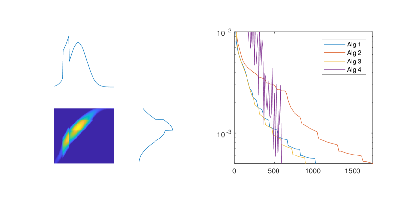
(a) $\gamma=50$

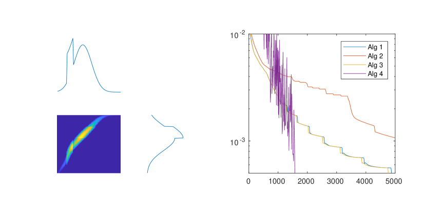
(b) $\gamma=10$

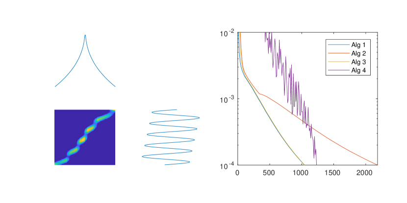
(c) $\gamma=10$

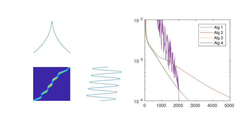
(d) $\gamma=4$

Figure 1: Results for one-dimensional examples with $c(x,y)=|x-y|^{2}$. Each subfigure on the left: Marginals and optimal plan. Each subfigure on the right: maximal violation of constraints over iteration count.

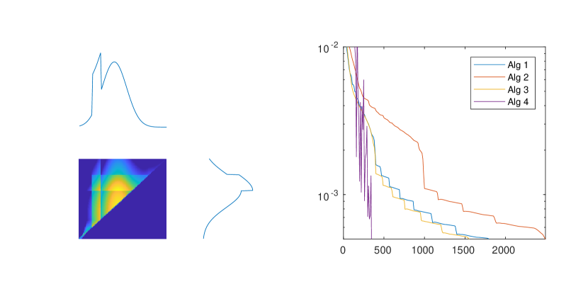
(a) $\gamma=100$

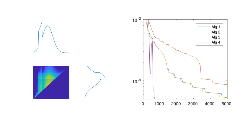
(b) $\gamma=50$

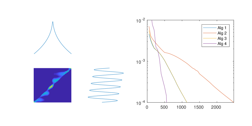
(c) $\gamma=50$

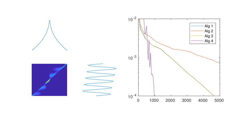
(d) $\gamma=15$

Figure 2: Results for one-dimensional examples with $c(x,y)=|x-y|$. Each subfigure on the left: Marginals and optimal plan. Each subfigure on the right: maximal violation of constraints over iteration count.

References

• [1] Hedy Attouch, Giuseppe Buttazzo, and Gérard Michaille. Variational Analysis in Sobolev and BV Spaces, volume 6 of MPS/SIAM Series on Optimization. Society for Industrial and Applied Mathematics (SIAM), Philadelphia, PA; Mathematical Programming Society (MPS), Philadelphia, PA, 2006.
• [2] Heinz H Bauschke, Jonathan M Borwein, and Adrian S Lewis. The method of cyclic projections for closed convex sets in hilbert space. Contemporary Mathematics, 204:1–38, 1997.
• [3] Jean-David Benamou, Guillaume Carlier, Marco Cuturi, Luca Nenna, and Gabriel Peyré. Iterative Bregman projections for regularized transportation problems. SIAM Journal on Scientific Computing, 37(2):A1111–A1138, 2015.
• [4] Colin Bennett and Robert Sharpley. Interpolation of Operators, volume 129 of Pure and Applied Mathematics. Academic Press, Inc., Boston, MA, 1988.
• [5] Mathieu Blondel, Vivien Seguy, and Antoine Rolet. Smooth and sparse optimal transport. arXiv preprint arXiv:1710.06276, 2017.
• [6] Christoph Brauer, Christian Clason, Dirk Lorenz, and Benedikt Wirth. A Sinkhorn-Newton method for entropic optimal transport. Proceedings of the Optimal Transport & Machine Learning workshop at NIPS 2017, 2017.
• [7] Guillaume Carlier, Vincent Duval, Gabriel Peyré, and Bernhard Schmitzer. Convergence of entropic schemes for optimal transport and gradient flows. SIAM Journal on Mathematical Analysis, 49(2):1385–1418, 2017.
• [8] Paola Cavaliere, Andrea Cianchi, Luboš Pick, and Lenka Slavíková. Norms supporting the lebesgue differentiation theorem. Communications in Contemporary Mathematics, 20(01):1750020, October 2017.
• [9] Christian Clason, Dirk A. Lorenz, Hinrich Mahler, and Benedikt Wirth. Entropic regularization of continuous optimal transport problems. arXiv preprint, 2019.
• [10] Marco Cuturi. Sinkhorn distances: Lightspeed computation of optimal transport. In Advances in neural information processing systems, pages 2292–2300, 2013.
• [11] Marco Cuturi and Gabriel Peyré. A smoothed dual approach for variational Wasserstein problems. SIAM J. Imaging Sci., 9(1):320–343, 2016.
• [12] Arnaud Dessein, Nicolas Papadakis, and Jean-Luc Rouas. Regularized optimal transport and the rot mover’s distance. The Journal of Machine Learning Research, 19(1):590–642, 2018.
• [13] Lars Diening, Petteri Harjulehto, Peter Hästö, and Michael Růžička. Lebesgue and Sobolev Spaces with Variable Exponents (Lecture Notes in Mathematics). Springer, 4 2011.
• [14] Ivar Ekeland and Roger Témam. Convex Analysis and Variational Problems, volume 28 of Classics in Applied Mathematics. Society for Industrial and Applied Mathematics (SIAM), Philadelphia, PA, 1999.
• [15] Dirk A Lorenz, Paul Manns, and Christian Meyer. Quadratically regularized optimal transport. arXiv preprint, 2019.
• [16] Gabriel Peyré and Marco Cuturi. Computational optimal transport. Foundations and Trends® in Machine Learning, 11(5-6):355–607, 2019.
• [17] M. M. Rao and Z. D. Ren. Theory of Orlicz Spaces. Pure and Applied Mathematics. Dekker, 1991.
• [18] Lucas Roberts, Leo Razoumov, Lin Su, and Yuyang Wang. Gini-regularized optimal transport with an application to spatio-temporal forecasting. arXiv preprint arXiv:1712.02512, 2017.
• [19] R. T. Rockafellar. Integrals which are convex functionals. Pacific J. Math., 24:525–539, 1968.
• [20] Filippo Santambrogio. Optimal Transport for Applied Mathematicians, volume 87 of Progress in Nonlinear Differential Equations and their Applications. Birkhäuser/Springer, Cham, 2015.
• [21] Richard Sinkhorn. A relationship between arbitrary positive matrices and stochastic matrices. Canad. J. Math., 18:303–306, 1966.
• [22] Richard Sinkhorn and Paul Knopp. Concerning nonnegative matrices and doubly stochastic matrices. Pacific J. Math., 21:343–348, 1967.
• [23] Cédric Villani. Topics in Optimal Transportation, volume 58 of Graduate Studies in Mathematics. American Mathematical Society, Providence, RI, 2003.
• [24] Cédric Villani. Optimal Transport. Old and New, volume 338 of Grundlehren der Mathematischen Wissenschaften [Fundamental Principles of Mathematical Sciences]. Springer-Verlag, Berlin, 2009.