Superfluid weight and polarization amplitude in the one-dimensional bosonic Hubbard model

Abstract

We calculate the superfluid weight and the polarization amplitude for the one-dimensional bosonic Hubbard model with focus on the strong-coupling regime via variational, exact diagonalization, and strong coupling calculations. Our variational approach is based on the Baeriswyl wave function, implemented via Monte Carlo sampling. We derive the superfluid weight appropriate in a variational setting. We emphasize the importance of implementing the Peierls phase in position space and to allow for many-body interference effects, rather than implementing the Peierls phase as single particle momentum shifts. At integer filling, the Baeriswyl wave function gives zero superfluid response at any coupling. At half-filling our variational superfluid weight is in reasonable agreement with exact diagonalziation results. We also calculate the polarization amplitude, the variance of the total position, and the associated size scaling exponent, which corroborate that this variational approach produces an insulating state at integer filling. Our Baeriswyl based variational method is applicable to significantly larger system sizes than exact diagonalization or quantum Monte Carlo.

I Introduction

The bosonic Hubbard model (BHM) was introduced by Gersch and Knollman Gersch63 to study the condensation of repulsive interacting bosons. The phase diagram of the superfluid-insulator transition was described by Fisher et al. Fisher89 . Since then the phase diagram has been calculated and refined by a variety of means, including mean-field theory Fisher89 ; Rokhsar91 , perturbative expansion Freericks96 , quantum Monte Carlo Batrouni90 ; Krauth91 ; Scalettar05 ; Rousseau06 ; Kashurnikov96b ; Rombouts06 (QMC), density matrix renormalization group Kuhner00 ; Ejima11 ; Zakrzewski08 ; Carrasquilla13 ; Kuhner98 , and exact diagonalization Kashurnikov96a . For a review see Ref.  Pollet12 . Due to the experimental realization of the model Jaksch98 ; Greiner02 as ultracold atoms in an optical lattice, the model has gained renewed interest.

The BHM is often applied to model Bose solids, e.g. solid ⁴He Anderson12 . One question of interest in these systems is under what conditions a superfluid type response is exhibited Reatto88 ; Vitiello88 . Some experimental Kim06 and some theoretical Galli05 results suggest that solid helium becomes supersolid at low temperatures. The experimental conclusions, some of which are based on torsional oscillator measurements, have since been challenged by the suggestion that other effects may be responsible for the observed drop in rotational inertia, such as quantum plasticity Beamish10 , moreover the role played by defects still awaits clarification (see Ref. Hallock15 for an overview). For the BHM Anderson Anderson12 has suggested that the ground state at integer filling is a supersolid.

In this work we apply a variational Monte Carlo Hetenyi16 for strongly correlated bosonic models based on the Baeriswyl wavefunction Baeriswyl86 ; Baeriswyl00 ; Dzierzawa97 ; Martelo97 ; Hetenyi10 ; Dora15 ; Yahyavi18 (BWF) and exact diagonalization (ED) to study the superfluid response and the polarization amplitude Resta98 ; Resta99 ; Aligia99 ; Souza00 ; Nakamura02 ; Yahyavi17 ; Kobayashi18 ; Hetenyi19 ; Nakamura19 ; Furuya19 of the one-dimensional BHM. Central to our study is the derivation of the expression for the superfluid weight valid in variational calculations, and emphasis of the role of interference between Peierls phases of particle paths in calculating the superfluid weight. According to our derivation, the Peierls phases should be implemented in position space, and phases along the paths of different particles should be allowed to interfere between exchanging particles. If the relevant propagators are Fourier transformed, and the Peierls phases are implemented as single-particle momentum shifts, interference effects are missed. The Fourier transform of the polarization amplitude shows a peak at small hopping strength for both the ED and the BWF-MC, which both decrease as the hopping strength is increased. This similarity is merely quantitative, the insulator-superfluid transition is only picked up in ED, where the scaling exponent of the variance of the polarization indicates gap closure. We also analyze Anderson’s treatment Anderson12 of the BHM in light of our findings.

Our paper is organized as follows. In the next section we present the model and the two methods used in this work, ED and the BWF-MC method. Subsequently, we discuss the superfluid weight. In section IV the polarization amplitude and cumulants are described. In section V our results are presented. In the penultimate section we comment on the calculation of the superfluid weight by Anderson, subsequently we conclude our work. A strong coupling treatment is presented in the Appendix.

II Model and methods

We study the BHM with nearest neighbor hopping in one dimension at fixed particle number. The Hamiltonian is

$$H=-J\sum_{i=1}^{L}\left(\hat{c}^{\dagger}_{i+1}\hat{c}_{i}+\hat{c}^{\dagger}_{i}\hat{c}_{i+1}\right)+U\sum_{i=1}^{L}\hat{n}_{i}(\hat{n}_{i}-1),$$ (1)

where $L$ denotes the number of sites, $J$ and $U>0$ are the hopping and repulsive on-site interaction parameters, respectively, $\hat{c}^{\dagger}_{i}$($\hat{c}_{i}$) denotes a bosonic creation(annihilation) operator at site $i$, and $\hat{n}_{i}$ denotes the density operator at site $i$.

While the method we developed is described in detail for the BWF elsewhere Hetenyi16 , here we describe aspects that are relevant to this study. The BWF has the form

$$|\Psi_{B}\rangle=\exp(-\alpha\hat{T})|\infty\rangle,$$ (2)

where $\alpha$ denotes the variational parameter, and $|\infty\rangle$ is the wavefunction at $U=\infty$. $\hat{T}$ denotes the hopping operator (first term in Eq. (1)). The crucial step in the construction of our method is that the kinetic energy propagator can be represented in real space as,

$$\langle x|\exp(-\alpha\hat{T})|x^{\prime}\rangle=\frac{1}{L}\sum_{k}e^{-\alpha\epsilon_{k}+ik(x-x^{\prime})},$$ (3)

where $\epsilon_{k}=-2J\cos(k)$. The full probability sampled Hetenyi16 consists of a product of single particle propagators. Bosonic exchanges have to be implemented by exchanging the positions of pairs of particles and accepting or rejecting such exchange moves.

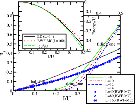
Figure 1: Superfluid weight based on exact diagonalization calculations and BWF-MC as a function of $J/U$ for different system sizes for fillings of one-half and one. The inset compares the energy per particle for integer filling for the Baeriswyl wave function based variational Monte Carlo method, exact diagonalization, and the strong coupling expansion based on the Baeriswyl wave function ($-2J^{2}/U$) for filling one.

For smaller systems, we diagonalize Eq. (1) by the well-known iterative Lánczos scheme. An important aspect of the method we use is the indexing of the states, which is based on the Lehmer combinatorial code Lehmer60 ; Laisant88 , a way to order permutations. This procedure is also called Ponomarev ordering Ponomarev09 ; Ponomarev10 ; Ponomarev11 and has been implemented in the BHM by Raventos et al. Raventos17 .

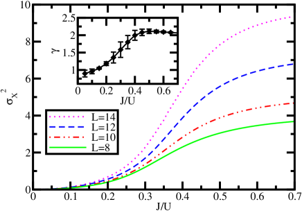
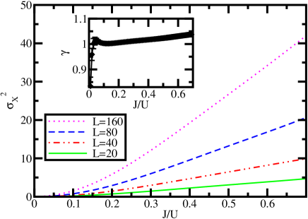
Figure 2: Second cumulant of the polarization as a function of $J/U$ for filling one for different system sizes based on exact diagonalization (upper panel) and variational Monte Carlo (lower panel) calculation. The inset shows the respective size scaling exponents.

III Superfluid weight

It is not immediately obvious that there is an issue with this quantity when it is considered specifically in a variational context. Usually the second derivative of the variational ground state energy with respect to the flux at zero Peierls flux is calculated Millis91 (see Eq. (13) for how the Peierls phase enters). One way to elucidate the issue Hetenyi14 is to consider that a variational estimate of the ground state energy is a weighted average of exact energy eigenvalues,

$$E_{var}=\sum_{i}P_{i}(\Phi)E_{i}(\Phi),$$ (4)

where $P_{i}=|\langle\Psi(\Phi)|\psi_{i}(\Phi)\rangle|^{2}$ ($|\Psi(\Phi)\rangle$ denotes the variational wave function, $|\psi_{i}(\Phi)\rangle$ denotes the $i$th eigenstate of the Hamiltonian), and $E_{i}(\Phi)$ denotes the $i$th energy eigenvalue. We argue here that the correct superfluid weight, when calculated in a variational calculation, is given by the expression

$$n_{S}=\frac{1}{L}\left.\sum_{i}P_{i}(\Phi)\frac{\partial^{2}E_{i}(\Phi)}{\partial\Phi^{2}}\right|_{\Phi=0},$$ (5)

in other words, the derivative of $P_{i}(\Phi)$ with respect to the flux need not be taken, in spite of its $\Phi$-dependence. However, in actual variational calculations, often neither $E_{i}(\Phi)$, nor $P_{i}(\Phi)$ are available, so we give an alternative, but equivalent expression for $n_{S}$, applicable in numerical settings.

Let us briefly recall the arguments of Pollock and Ceperley Pollock87 . In their work a continuous system of interacting atoms is considered, at finite temperature. Below we modify their steps to account for our lattice model. Pollock and Ceperley Pollock87 considered a thought experiment, aimed to mimic the rotating bucket experiments on superfluids. In this setup, the sample is rotated and the rotational inertia is measured. Below the critical temperature, where the superfluid fraction ceases to rotate with the container, the rotational inertia takes a non-classical value Fisher73 ; Rousseau14 , different from the rotational inertia calculated from the amount of fluid present in the container. In the context of supersolidity Leggett suggested Leggett70 that torsional oscillator experiments can access the rotational inertia, and therefore the superfluid weight.

In Ref. Pollock87 the sample is enclosed between a two circular walls, one of radius $R$, the other of radius $R+d$. When $R\gg d$, the system becomes equivalent to the sample between two parallel planes. In the experiment the walls are moved by an outside agent with velocity $v$. It is expected that the normal component of the fluid will move with the walls, due to friction, while the superfluid component will remain stationary in the laboratory frame.

The density matrix of the system is

$$\hat{\rho}_{v}=\exp(-\beta\hat{H}_{v}),$$ (6)

where $\beta$ denotes the inverse temperature, and

$$\hat{H}_{v}=\sum_{j=1}^{N}\frac{(\hat{p}_{j}-mv)^{2}}{2m}+\hat{V},$$ (7)

where $\hat{p}_{j}$ denotes the momentum of an individual particle, $m$ denotes the mass of a particle, and $\hat{V}$ denotes an interaction. The total momentum of the system (the momentum of the normal component) is given by

$$\frac{\rho_{n}}{\rho}Nmv=\frac{\mbox{Tr}\{\hat{\rho}_{v}\hat{P}\}}{\mbox{Tr}\{\hat{\rho}_{v}\}},$$ (8)

where $\rho_{n}$ denotes the density of the normal phase, $\rho$ denotes the total density, and

$$\hat{P}=\left.\frac{\partial{\hat{H}_{v}}}{\partial v}\right|_{v=0}=\sum_{j=1}^{N}\hat{p}_{j}.$$ (9)

We can write the free energy of the system as

$$\exp(-\beta F_{v})=\mbox{Tr}\{\exp(-\beta\hat{H}_{v})\}.$$ (10)

Taking the first derivative of $F_{v}$ with respect to $v$ results in

$$\frac{\partial F_{v}}{\partial v}=Nmv\left(1-\frac{\rho_{n}}{\rho}\right),$$ (11)

resulting in the superfluid weight of

$$\frac{\rho_{s}}{\rho}=\frac{1}{Nm}\left.\frac{\partial^{2}F_{v}}{\partial v^{2}}\right|_{v=0}.$$ (12)

In a lattice model the analog of the velocity $v$ is the Peierls phase, which we introduce into the Hamiltonian as

$$H(\Phi)=-J\sum_{i=1}^{L}\left(e^{i\Phi}\hat{c}^{\dagger}_{i+1}\hat{c}_{i}+e^{-i\Phi}\hat{c}^{\dagger}_{i}\hat{c}_{i+1}\right)+U\sum_{i=1}^{L}\hat{n}_{i}(\hat{n}_{i}-1).$$ (13)

In exact diagonalization calculations, the analog of Eq. (12), the superfluid weight, is obtained by calculating the response of the system to the Peierls phase (or boundary twist) as,

$$n_{S}=\frac{1}{L}\left[\frac{\partial^{2}E_{g}(\Phi)}{\partial\Phi^{2}}\right]_{\Phi=0}.$$ (14)

Here $E_{g}(\Phi)$ denotes the ground state of the system, since our lattice system is studied at zero temperature.

In the BWF-MC method we use, where the exact eigenenergies are not available, it is not possible to calculate the superfluid weight directly (via Eq. (14)). Instead we derive the superfluid weight in a variational context based on the reasoning of Pollock and Ceperley Pollock87 . Our starting point is the normalization of the Baeriswyl wavefunction,

$$\tilde{Q}_{\Phi}=\langle\infty|\exp\left(-2\alpha\hat{T}(\Phi)\right)|\infty\rangle=\exp(-2\alpha\tilde{F}_{\Phi}),$$ (15)

which is analogous to the partition function in statistical mechanics. We also defined $\tilde{F}_{\Phi}$, the “free energy” in the variational context. The analog of Eq. (11) is

$$\frac{\partial\tilde{F}_{\Phi}}{\partial\Phi}=\cos\Phi J_{\Phi}-\sin\Phi T_{\Phi},$$ (16)

where

$$J_{\Phi}=\langle\infty|\exp\left(-\alpha\hat{T}(\Phi)\right)\hat{J}\exp\left(-\alpha\hat{T}(\Phi)\right)|\infty\rangle,$$ (17)

with the current operator $\hat{J}$ being

$$\hat{J}=\left.\frac{\partial H(\Phi)}{\partial\Phi}\right|_{\Phi=0}=-2J\sum_{k}\sin(k)n_{k},$$ (18)

and

$$T_{\Phi}=\langle\infty|\exp\left(-\alpha\hat{T}(\Phi)\right)\hat{T}\exp\left(-\alpha\hat{T}(\Phi)\right)|\infty\rangle,$$ (19)

with $\hat{T}$ indicating the hopping energy operator at zero flux. Note that $\hat{J}$ is the lattice analog of the total momentum operator (compare Eq.(18) and Eq. (9)).

From Eq. (11), we derive our proposed expression for the superfluid weight for variational calculations,

$$n_{S}=\frac{1}{L}\left.\frac{\partial^{2}\tilde{F}_{\Phi}}{\partial\Phi^{2}}\right|_{\Phi=0}=\frac{1}{L}\left(\frac{\partial J_{0}}{\partial\Phi}-T_{0}\right).$$ (20)

In the case of an exact eigenstate, this expression corresponds to Eq. (14), but in the case of a weighted average of the type in Eq. (4) it corresponds to Eq. (5). To see this, we first write $T_{0}$ as

$$T_{0}=\sum_{i}P_{i}T_{i}$$ (21)

where $T_{i}$ denotes the expectation value of the kinetic energy in eigenstate $i$, and write $J_{\Phi}$ as

$$J_{\Phi}=\sum_{i}P_{i}(\Phi)J_{i}(\Phi),$$ (22)

where $J_{i}(\Phi)$ denotes the expectation value of the current operator ($\hat{J}$) in the eigenstate $|\psi_{i}(\Phi)\rangle$, and take the derivative with respect to $\Phi$, resulting in

$$\frac{\partial J_{\Phi}}{\partial\Phi}=\sum_{i}\left[\frac{\partial P_{i}(\Phi)}{\partial\Phi}J_{i}(\Phi)+P_{i}(\Phi)\frac{\partial J_{i}(\Phi)}{\partial\Phi}\right].$$ (23)

Setting $\Phi=0$, we can use the fact that $J_{i}(0)=0$, leaving us with

$$n_{S}=\frac{1}{L}\sum_{i}P_{i}\left(\frac{\partial J_{i}(0)}{\partial\Phi}-T_{i}\right),$$ (24)

which is exactly Eq. (5).

The second derivative in Eq. (20) involves two limits, $\Phi\rightarrow 0$ and $L\rightarrow\infty$. In one dimension the order of limits is inconsequential, the superfluid weight is obtained in both cases Scalapino92 ; Scalapino93 . Below we evaluate the second derivative in Eq. (20) by way of finite difference on a grid $\Phi=m2\pi/L$, with $m$ integer.

Some care needs to be exercised in applying the derivative with respect to $\Phi$. It appears highly tempting to implement the Peierls phase as a shift in $k$, as $\epsilon_{k}\rightarrow\epsilon_{k+\Phi}$ in each single particle propagator (Eq. (3)). This approach leads to a finite superfluid weight even at integer filling. However, in this case the interference between the particles is neglected.

To elaborate, let us write $\tilde{Q}_{\Phi}$ in the coordinate representation as

$$\tilde{Q}_{\Phi}=\sum_{\bf x_{L},x_{R}}\langle\infty|{\bf x_{L}}\rangle\langle{\bf x_{L}}|\exp\left(-2\alpha\hat{T}(\Phi)\right)|{\bf x_{R}}\rangle\langle{\bf x_{R}}|\infty\rangle,$$ (25)

where ${\bf x_{L/R}}=x_{L/R,1},...,x_{L/R,N}$, indicating particle positions in the “left” or “right” coordinate bases. For the moment, let us consider a one-particle propagator,

$$\langle x|\exp\left(-2\alpha\hat{T}(\Phi)\right)|x^{\prime}\rangle=\langle x|(1-2\alpha\hat{T}(\Phi)+2\alpha^{2}\hat{T}(\Phi)\hat{T}(\Phi))|x^{\prime}\rangle$$ (26)

A term in which the difference between $x^{\prime}$ and $x$ is a fixed number will involve all different paths which go from $x$ to $x^{\prime}$. The different paths may have a different number of hoppings, left and right, but the difference between $x^{\prime}$ and $x$ is the same. Each right hopping contributes a phase of $\Phi$, while each left hopping contributes a phase of $-\Phi$. Thus, the net change in phase will be determined solely by $x^{\prime}-x$, we can write,

$$\langle x|\exp\left(-2\alpha\hat{T}(\Phi)\right)|x^{\prime}\rangle= \exp\left[i\Phi(x^{\prime}-x)\right]\times$$

$$\langle x|\exp\left(-2\alpha\hat{T}(0)\right)|x^{\prime}\rangle.$$

We used the fact that for a periodic system $\langle x|x^{\prime}\rangle=\delta_{x,x^{\prime}+L}$. Armed with this, we can rewrite $\tilde{Q}(\Phi)$ as

$$\tilde{Q}_{\Phi}=\sum_{\bf x_{L},x_{R}}\exp\left[i\Phi\sum_{i=1}^{N}(x_{R,i}-x_{L,i})\right]\times$$ (28)

$$\hskip 14.22636pt\langle\infty|{\bf x_{L}}\rangle\langle{\bf x_{L}}|\exp\left(-2\alpha\hat{T}(0)\right)|{\bf x_{R}}\rangle\langle{\bf x_{R}}|\infty\rangle.$$

We note that the operator appearing in the exponential $\sum_{i=1}^{N}(x_{R,i}-x_{L,i})$ is a sum of differences between single particle positions. The contribution from different particles are now added, and they can cancel. The position operator is undefined in a periodic system, but its exponential, provided that $\Phi=m2\pi/L$ is well-defined. Such an operator is used in the many-body analog of the modern theory of polarization Resta98 ; Resta99 , also to express a second derivative in the momentum shift Hetenyi19 . Following the same steps, we can write

$$n_{S}=-\lim_{L\rightarrow\infty}\left[\frac{L^{2}}{4\alpha\pi^{2}}\right]\mbox{Re}\ln\tilde{Q}_{2\pi/L}$$ (29)

If the system has integer filling, it always holds that

$$\sum_{i=1}^{N}(x_{R,i}-x_{L,i})=0,$$ (30)

leading to a superfluid weight of zero. According to this derivation a finite superfluid weight can only arise for non-integer fillings. This coincides with previous results on the Drude weight of the Baeriswyl wave function in fermionic systems Dzierzawa97 .

The derivation we provided above is specific to the BWF, in which the hopping energy appears explicitly in the projector. In variational wave functions where that is not the case, one has to apply a Baeriswyl projector, threaded by a Peierls flux, and take the limit of $\alpha\rightarrow 0$ in the final expression for $n_{S}$.

IV Polarization amplitude

For a periodic lattice system the total position operator is ill-defined. In a many-body system the standard approach  Resta98 is to calculate the expectation value of the twist operator Lieb61 , also known as the polarization amplitude Kobayashi18 ,

$$Z_{q}=\langle\Psi|\exp\left(i\frac{2\pi q}{L}\hat{X}\right)|\Psi\rangle.$$ (31)

where $\hat{X}=\sum_{i=1}^{N}x_{i}\hat{n}_{i}$. This quantity can be interpreted as a characteristic function, and derivatives with respect to $q$ give the average of $\hat{X}$, the variance of $\hat{X}$ or higher order cumulants. The second cumulant, $\sigma^{2}_{N}$, which measures the spread of the center of mass, can be used to determine whether a system is a conductor or an insulator Kohn64 ; Resta98 ; Resta99 ; Souza00 ; Yahyavi17 . In a finite system the definition of the spread is

$$\sigma^{2}_{N}=-\frac{L^{2}}{4\pi^{2}}\left.\frac{\Delta^{2}\ln Z_{q}}{\Delta q^{2}}\right|_{q=0},$$ (32)

where $\frac{\Delta G}{\Delta q}$ indicates a discrete derivative of $G$ with respect to $q$. While the commonly used expression for the variance of the total position of Resta and Sorella is Resta98 ; Resta99 , $\sigma^{2}=-\frac{L^{2}}{2\pi^{2}}\mbox{Re}\ln Z_{1},$ (consistent with Eq. (32)), for small system sizes scaling exponents are difficult to obtain from Eq. (32). A simple remedy Hetenyi19 is to take the derivative of the ln function analytically, and apply discrete derivatives to the remaining cases,

$$\sigma^{2}_{N}=-\frac{L^{2}}{4\pi^{2}}\left[\left(\left.\frac{\Delta^{2}Z_{q}}{\Delta q^{2}}\right|_{q=0}\right)-\left(\left.\frac{\Delta Z_{q}}{\Delta q}\right|_{q=0}\right)^{2}\right].$$ (33)

In our calculations below we will use Eq. (33) to calculate the variance and the size scaling exponent $\gamma$ from an assumed scaling form of

$$\sigma^{2}_{N}(L)=aL^{\gamma}.$$ (34)

We also calculate the discrete Fourier transform of $Z_{q}$, which we define as

$$\tilde{Z}_{x}=\sum_{q=1}^{L}\exp\left(i\frac{2\pi qx}{L}\right)Z_{q},$$ (35)

where $x=1,...,L$.

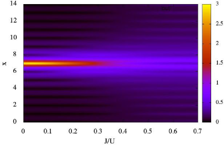
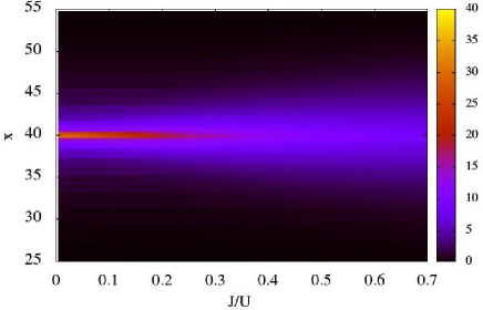
Figure 3: $\tilde{Z}_{x}$, the Fourier transform of the function $Z_{q}$, as a function of $x$ (the variable conjugate to $q$) and $J/U$ for a system of filling one. Upper panel: exact diagonalization ($L=14$), lower panel: BWF-MC ($L=80$).

V Numerical Results

Fig. 1 shows the superfluid weight for systems of different system sizes at filling one-half and one. The half-filled system is always superfluid. The BWF-MC and ED results are reasonably close in the case of half filling. For integer filling only the ED results are shown, since the BWF-MC are zero, as shown above. The ED results show no superfluid response for small hopping values up to $J/U\sim 0.2$. At that point the superfluid weight starts to grow for the smallest system size. Larger system sizes persist in an insulating state until larger values of $J/U$, but all of them are noticeable by $J/U\approx 0.3$. In the half-filled system the energy as a function of $\Phi$ was found to be discontinuous at a finite value of $\Phi$, indicating a level crossing. No level crossing was found for filling one. We note that at filling one the gap closure (corresponding to the Kosterlitz-Thouless transition) occurs Kuhner00 ; Ejima11 ; Zakrzewski08 ; Kashurnikov96a at $(J/U)_{KT}\approx 0.6$. In particular, the ED calculation extended by a renormalization group analysis by Kashurnikov and Svistunov Kashurnikov96a gives $J_{KT}=0.608(4)$, nearly twice the value where the superfluid weight begins to grow in Fig. 1. Actually, for hopping value $J/U\sim 0.3-0.5$, ED indicates a non-zero superfluid weight, but this is not a reliable result, once we are approaching a quantum transition, $(J/U)_{KT}\approx 0.6$, and the smallness of the system sizes, up to $L=14$, becomes highly manifest.

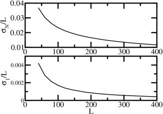
Figure 4: Standard deviation of the position (divided by the system size) vs. system size, for a system with $J/U=0.25$ at filling one. Upper panel: total position for a bosonic system, lower panel: single-particle position with bosonic exchange moves turned off.

In Fig. 2 the variance of the total position $\sigma^{2}_{N}$ and its size scaling exponent $\gamma$ are shown. The size scaling exponent $\gamma$ is shown in the insets. The size scaling exponent $\gamma$ is known Hetenyi19 to take the value two in a closed gap (conducting) system, and the value one for an insulating system. We notice that in the upper panel of Fig. 2, the exact diagonalization calculations bear out these expectations, notwithstanding the limitations of small system sizes. The scaling exponent $\gamma$ is near the value one when $J/U$ is small, and increases to two around $J/U\sim 0.5$, in reasonable agreement with the results of Kashurnikov and Svistunov Kashurnikov96a . For the BWF-MC calculations (lower panel of Fig. 2), the size scaling exponent is near one, in agreement with what is expected for an insulating phase. As argued in section III the superfluid weight is zero for the Baeriswyl wave function at integer filling. This conclusion is corroborated by our variational results shown in the inset of the lower panel of Fig. 2.

The upper panel of Fig. 3 shows $\tilde{Z}_{x}$, the discrete Fourier transform of $Z_{q}$ in the form of a color map $(J/U$ is the variable on the $x$-axis, the variable conjugate to $\tilde{Z}_{x}$ is on the $y$-axis). The system is the unit filled one. The interesting result on this figure is the peak, which occurs at $x=7$, half the unit cell, which is where it should be for a half-filled system with no spontaneous polarization. The peak is relatively constant until $J/U\approx 0.3$, then starts to decrease. Again, this occurs at $J/U$ where the superfluid weight increases in Fig. 1. The lower panel of Fig. 3 show $\tilde{Z}_{x}$ as a function of $x$ and $J/U$ based on our variational Monte Carlo results. The similarity between the upper and lower panels are striking: a sharp peak half-way through the supercell exists near $J=0$, which decreases around $J/U\approx 0.3$. An important difference between the two results is the scaling of the spread of the distributions, shown in the insets of Fig. 2. Inspite of the qualitative similarity, the two distributions are indicative of different physical behavior.

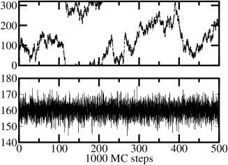
Figure 5: Upper panel: position of one particle on the lattice, lower panel: total position modulo the size of the system, for a system with $J/U=0.25$, $N=320$ particles, and size $L=320$ lattice sites.

In order to analyze the behavior of the superfluid weight (next section), we present two more sets of results in Figs. 4 and 5. The former shows the spread of the position as a function of system size $J/U=0.25$ for two cases, both at filling one. In the upper panel the total position is shown, indicating convergence with system size, or insulating behavior. In the lower panel, we show the variance in the position of one particle, when bosonic exchange moves are turned off (in other words, in a system of distinguishable particles). Fig. 5 shows two time series in the course of the MC simulation, the upper panel for the position of a single particle (with bosonic exchange moves), the lower panel for the total position. We see that even though the single particle delocalizes over the whole lattice, the total position fluctuates around the center of the unit cell. We see that bosonic exchange delocalizes single particles, but leaves the center of mass localized, fluctuating around the center of the supercell. Similarly, a superfluid weight calculation which neglects the interference of particles would lead to a finite superfluid response (we checked this).

VI Discussion

Anderson has argued Anderson12 , based on a strong coupling expansion, that the superfluid response of the BHM is finite at integer filling. Here, we show that his formalism is similar to our strong-coupling expansion, and that his way of implementing the Peierls flux does not allow for interference between particles. The finite superfluid weight is an artifact of this implementation.

We follow the steps of  Anderson12 , but we a a system threaded by a flux $\Phi$ at the outset. For filling one in the strong coupling limit $U\gg J$ and up to the leading order in $J/U$, the many-body ground state is written as the product of non-orthogonal bosons, the so called ”eigenbosons”,

$$|\Psi_{A}(\Phi)\rangle=\prod_{i=1}^{L}{{\hat{b}}^{\dagger}_{i}(\Phi)}|0\rangle$$ (36)

where the ”eigenbosons” are given by,

$${\hat{b}}^{\dagger}_{i}(\Phi) =\frac{1}{M}\left[{\hat{c}}^{\dagger}_{i}+e^{-i\Phi}\frac{J}{2U}{\hat{c}}^{\dagger}_{i+1}+e^{i\Phi}\frac{J}{2U}{\hat{c}}^{\dagger}_{i-1}\right]$$ (37)

with $M=\sqrt{1+2(J/2U)^{2}}$. Let us write down the first few terms of Eq. (36). The zeroth order term is

$$\prod_{i}\hat{c}_{i}^{\dagger}|0\rangle$$ (38)

which is equal to $|\infty\rangle$, the term zeroth order in $J/U$ in Eq. (50). The term first order in $J/U$ is

$$\frac{J}{2U}\sum_{i}[\exp(i\Phi)\hat{c}^{\dagger}_{i+1}+\exp(-i\Phi)\hat{c}^{\dagger}_{i-1}]\prod_{j\neq i}c_{j}^{\dagger}|0\rangle,$$ (39)

which is exactly the first order term in Eq. (50). For this system we calculated the ground state energy, and showed that the superfluid weight is zero.

The particular steps of Anderson, leading to the supefluid weight, are as follows. The bosonic states are Fourier transformed as,

$$\hat{b}_{0} = \hat{c}_{0}+\left(\frac{Je^{-i\Phi}}{2U}\hat{c}_{1}+\frac{Je^{i\Phi}}{2U}\hat{c}_{-1}\right)$$

$$= \frac{1}{\sqrt{L}}\sum_{k}\left[1+(J/U)\cos(k+\Phi)\right]\hat{c}_{k}.$$

The kinetic energy is written

$$K=-\frac{J}{N}\sum_{k}\cos(k+\Phi)[1+2(J/U)\cos\Phi\cos k+(J/U)^{2}\cos^{2}k]$$ (41)

The second derivative of $K$ according to $\Phi$ will give a finite contribution. The issue is that in the Fourier transform of Eq. (VI), the Peierls phase is separated from the rest of the system (in the words of Anderson a pair of lattice sites is “embedded” in the system), and not allowed to interfere with the Peierls phases of other hoppings. When, in our BWF-MC calculations, a Peierls phase is implemented in each of the propagators independently, without interference, a finite superfluid weight also results. Moreover, at small $J/U$ the two results give the same scaling with $J/U$.

VII Conclusion

In the context of solid ⁴He supersolidity was suggested by Kim and Chan Kim06 based on torsional oscillator experiments. It is important to note that while the bosonic Hubbard model may give useful hints into the behavior of solid helium, some aspects, for example vacancies and dislocations, are not accounted for Chan13 . The experiments of Kim and Chan were also brought in to question by the suggestion Beamish10 that their results could be due to quantum plasticity. Quantum plasticity is a phenomenon which can only be defined in more than one dimension.

Our studies show that the Baeriswyl wave function can not produce a finite superfluid weight. Interestingly, the Fourier transform of the polarization amplitude behaves very similarly to its counterpart calculated by exact diagonalization. Closer inspection however, for example, the calculation of the size scaling exponent, still indicates an insulating system. Therefore, the BWF is reliable up to $J/U\approx 0.5$ not only for the ground state energy, but also for the polarization amplitude in the insulating phase.

We also stressed the proper way to calculate the superfluid weight in a variational context and commented on a calculation of Anderson based on which a finite superfluid response was found for the integer filled bosonic Hubbard model. Our central result is that the “usual” formula of the superfluid weight, the second derivative with respect to a momentum shifting Peierls phase, is not directly applicable in a variational context.

Appendix:Strong coupling expansion based on the Baeriswyl wave function

The BHM has been studied via a number of strong coupling expansions Freericks96 ; Elstner99 ; Damski06 ; Krutitsky08 ; Heil12 . Such expansions in the case of the BHM are usually more difficult than in the case of the fermionic Hubbard model, where the Heisenberg model is obtained as the limiting case.

In the atomic limit, the 1D BHM ground state at filling one is given by a full localized boson state

$$|\infty\rangle=\prod_{i=1}^{L}{\hat{c}}_{i}^{\dagger}|0\rangle.$$ (42)

Threading the system with a flux $\Phi$, using the fact that the state $|\Psi_{\infty}\rangle$ is not $\Phi$ dependent, the BWF reads

$$|\Psi_{B}(\Phi)\rangle=\exp(-\alpha\hat{T}(\Phi))|\infty\rangle$$ (43)

where $\hat{T}(\Phi)$ is the first term in the r.h.s. of Eq. (13). Our first aim is to evaluate the variational energy,

$$E_{B}(\alpha,\Phi)=\frac{\langle\Psi_{B}(\Phi)|{\hat{H}}(\Phi)|\Psi_{B}(\Phi)\rangle}{\langle\Psi_{B}(\Phi)|\Psi_{B}(\Phi)\rangle},$$ (44)

by performing a strong-coupling expansion ($J/U\ll 1$) via expanding the kinetic projector and keeping the leading order terms in $J/U$ in all relevant quantities. An important point is that successive applications of the kinetic operator on $|\infty\rangle$ (a state with all sites occupied by one particle) in expectation values of the type in Eq. (44) should be such that one returns to the state $\langle\infty|$.

Up to first order in $J/U$ the BWF is given by

$$|\Psi_{B}(\Phi)\rangle =|\infty\rangle+\alpha J|\Psi_{d}(\Phi)\rangle$$ (45)

where $|\Psi_{d}(\Phi)\rangle=\sum_{i=1}^{L}\left(e^{i\Phi}\hat{c}^{\dagger}_{i+1}\hat{c}_{i}+e^{-i\Phi}\hat{c}^{\dagger}_{i}\hat{c}_{i+1}\right)|\Psi_{\infty}\rangle$, a state which is a superposition of states with occupation number $n_{i}$ being $0$ and $2$ for a pair of nearest neighboring sites and $1$ for all other sites.

The pair occupation, needed for the potential energy, within our approximation is given by

$$n_{p}=\langle\Psi_{B}(\Phi)|{\hat{n}}_{i}({\hat{n}}_{i}-1)|\Psi_{B}(\Phi)\rangle=8\alpha^{2}J^{2}$$ (46)

and the average of the potential energy by

$$\langle\Psi_{B}(\Phi)|{\hat{U}}|\Psi_{B}(\Phi)\rangle=8\alpha^{2}J^{2}UL$$ (47)

where ${\hat{U}}$ is the second term in the r.h.s. of Eq. (1). The boson momentum distribution reads

$$n(k,\Phi)=\langle\Psi_{B}(\Phi)|{\hat{n}}_{k}|\Psi_{B}(\Phi)\rangle=1+8\alpha J\cos(k+\Phi)\\$$ (48)

where ${\hat{n}}_{k}={\hat{c}}_{k}^{\dagger}{\hat{c}}_{k}$ and $\hat{c}^{\dagger}_{k}=\frac{1}{\sqrt{L}}\sum_{i=1}^{L}e^{-ikx_{i}}\hat{c}^{\dagger}_{i}$. The above result is obtained by performing the calculations in momentum space and exponentials $e^{\pm i(k+\Phi)}$ lead to the momentum distribution to depend on $k+\Phi$. The average of the kinetic energy is

$$\langle\Psi_{B}(\Phi)|{\hat{T}}(\Phi)|\Psi_{B}(\Phi)\rangle=\sum_{k}\epsilon_{k+\Phi}n(k,\Phi)=-8\alpha J^{2}L$$ (49)

Note that both $\epsilon_{k+\Phi}$ and $n(k,\Phi)$ depend on $k+\Phi$, therefore the kinetic energy is not flux dependent as expected, since, at filling one, the product $\epsilon_{k+\Phi}n(k,\Phi)$ just represents an overall shift in the Brillouin zone relatively to system without flux. Optimizing the total energy at any flux leads to $\alpha^{*}=\frac{1}{2U}$. The optimal variational wavefunction is given by

$$|\Psi_{B}(\Phi,\alpha^{*})\rangle=|\infty\rangle+\frac{J}{2U}|\Psi_{d}(\Phi)\rangle$$ (50)

and the ground state energy per site by

$$E_{B}(\alpha^{*})=-\frac{2J^{2}}{U},$$ (51)

where we dropped the $\Phi$ dependence from the notation. The inset in Fig. 1 compares this approximation to the results of exact diagonalization for fourteen sites, and BWF-MC results for a system of $L=160$.

As for the superfluid weight (Eq. (20)), we first express the total current operator under a flux $\Phi$ within our approximation as

$${\hat{J}}(\Phi) = \frac{\partial{\hat{T}}(\Phi)}{\partial\Phi}=2J\sum_{k}\sin(k+\Phi)\hat{c}^{\dagger}_{k}\hat{c}_{k},$$ (52)

and its average over $|\Psi_{B}(\Phi)\rangle$ is zero

$$J_{\Phi}(\Phi)=2J\sum_{k}\sin(k+\Phi)n(k,\Phi)=0$$ (53)

indicating the insulating character of $|\Psi_{B}(\Phi)\rangle$ at filling one. The average of the current operator expressed by Eq. (17) reads

$$J_{\Phi} = 2J\sum_{k}\sin(k)n(k,\Phi)=-\frac{4J^{2}}{U}\sin\Phi L$$ (54)

while the average of the kinetic energy, expressed by Eq. (19) reads

$$T_{\Phi}=\sum_{k}\epsilon(k)n(k,\Phi)=-\frac{4J^{2}}{U}\cos\Phi L$$ (55)

Using Eq. (20) $n_{S}=0$ for the BHM at filling one in the strong coupling expansion, in agreement with the previous ED and BWF-MC results.

For the 1D BHM at filling one up to order in $(J/U)^{2}$, the kinetic and potential energy per site averages (at optimal variational parameter), read $\langle{\hat{T}}\rangle=-\frac{4J^{2}}{U}$ and $\langle{\hat{U}}\rangle=\frac{2J^{2}}{U}$, respectively. Physically, this means that, through the kinetic exchange mechanism, the kinetic energy gain is bigger than the on-site potential energy cost, in perfect analogy with the Fermionic Hubbard Model (FHM) in the strong coupling limit Fazekas99 . Along the same lines, the pair occupancy, Eq. (46), and momentum distribution for $\Phi=0$, Eq. (48), read as

$$n_{p} = \frac{2J^{2}}{U^{2}}$$ (56)

and

$$n(k)=1-\frac{2\epsilon_{k}}{U}$$ (57)

also in perfect analogy with the FHM in the strong coupling limit, except, obviously, for the absence of the spin-spin term Fazekas99 . It is also worth mentioning that the momentum distribuition for $\Phi=0$, Eq. (57), is in agreement with that of Ref. trivedi2009 .

References

- (1) H. Gersch and G. Knollmann Phys. Rev., 129 959 (1963).
- (2) M. P. A. Fisher, P. B. Weichman, G. Grinstein, and D. S. Fisher, Phys. Rev. B, 40 546 (1989).
- (3) D. S. Rokhsar and B. G. Kotliar Phys. Rev. B, 44 10328 (1991).
- (4) J. K. Freericks and H. Monien Phys. Rev. B, 53 2691 (1996).
- (5) G.G. Batrouni, R. T. Scalettar, and G. T. Zimányi, Phys. Rev. Lett., 65 1765 (1990).
- (6) W. Krauth, and N. Trivedi, Europhys. Lett. 14 627 (1991).
- (7) R. T. Scalettar, G. Batrouni, P.J.H. Denteneer, F. Hébert, A. Muramatsu, M. Rigol, V. G. Rousseau et M. Troyer, J. Low Temp. Phys., 140 315 (2005).
- (8) V. G. Rousseau, D. P. Arovas, M. Rigol, F. Hébert, G. G. Batrouni, and R. T. Scalettar, Phys. Rev. B, 73 174516 (2006).
- (9) V. A. Kashurnikov, A. V. Kravasin, B. V. Svistunov, JETP Lett. 64 99 (1996).
- (10) S. M. A. Rombouts, K. Van Houcke, and L. Pollet, Phys. Rev. Lett. 96 180603 (2006).
- (11) T. D. Kühner, S. R. White, and H. Monien, Phys. Rev. B, 61 12474 (2000).
- (12) S. Ejima, H. Fehske, and F. Gebhard, EPL 93 30002 (2011).
- (13) J. Zakrzewski and D. Delande, AIP Conf. Proc. 1076 292 (2008).
- (14) J. Carrasquilla, S. R. Manmana, and M. Rigol, Phys. Rev. A 87 043606 (2013).
- (15) T. D. Kühner, and H. Monien, Phys. Rev. B, 58 R14741 (1998).
- (16) V. A. Kashurnikov and B. V. Svistunov, Phys. Rev. B 53 11776 (1996).
- (17) L. Pollet, Rep. Prog. Phys., 75 094501 (2012).
- (18) D. Jaksch, C. Bruder, J. I. Cirac, C. W. Gardiner, P. Zoller, Phys. Rev. Lett., 81 3108 (1998).
- (19) M. Greiner, O. Mandel, T. Esslinger, T. W. Hänsch, I. Bloch, Nature, 415 39 (2002).
- (20) P. W. Anderson, J. Low Temp. Phys. 169 124 (2012); arXiv.org:1102.4797.
- (21) L. Reatto and G. L. Masserini, Phys. Rev. B, 38 4516 (1988)
- (22) S. Vitiello, K. Runge, and M. H. Kalos, Phys. Rev. Lett., 60 1970 (1988).
- (23) E. Kim and M. H. W. Chan, Phys. Rev. Lett., 97 115302 (2006).
- (24) D. E. Galli, M. Rossi, and L. Reatto, Phys. Rev. B, 71 140506(R) (2005).
- (25) J. R. Beamish, Physics 3 51 (2010).
- (26) R. Hallock, Physics Today, 68 30 (2015).
- (27) B. Hetényi, B. Tanatar, and L. M. Martelo, Phys. Rev. B 93 174518 (2016).
- (28) D. Baeriswyl in Nonlinearity in Condensed Matter, Ed. A. R. Bishop, D. K. Campbell, D. Kumar, and S. E. Trullinger, Springer-Verlag (1986).
- (29) D. Baeriswyl, Found. Physics, 30 2033 (2000).
- (30) M. Dzierzawa, D. Baeriswyl, and L. M. Martelo, Helv. Phys. Acta, 70 124 (1997).
- (31) L. M. Martelo, M. Dzierzawa, L.Siffert, and D. Baeriswyl, Z. Phys. B, 103, 335 (1997).
- (32) B. Hetényi, Phys. Rev. B, 82 115104 (2010).
- (33) B. Dóra, M. Haque, F. Pollmann and B. Hetényi , Phys. Rev. B 93 115124 (2016).
- (34) M. Yahyavi, L. Saleem, and B. Hetényi , J. Phys. Cond. Mat. 30 445602 (2018).
- (35) R. Resta, Phys. Rev. Lett. 80 1800 (1998).
- (36) R. Resta and S. Sorella, Phys. Rev. Lett. 82 370 (1999).
- (37) A. A. Aligia and G. Ortiz, Phys. Rev. Lett. 82 2560 (1999).
- (38) I. Souza, T. Wilkens, and R. M. Martin, Phys. Rev. B 62 1666 (2000).
- (39) M. Nakamura and J. Voit, Phys. Rev. B 65 153110 (2002).
- (40) M. Yahyavi and B. Hetényi, Phys. Rev. A 95 062104 (2017).
- (41) R. Kobayashi, Y. O. Nakagawa, Y. Fukusumi, M. Oshikawa, Phys. Rev. B 97 165133 (2018).
- (42) B. Hetényi and B. Dóra, Phys. Rev. B 99 085126 (2019).
- (43) M. Nakamura and S. C. Furuya, Phys. Rev. B 99 075128 (2019).
- (44) S. C. Furuya and M. Nakamura, Phys. Rev. B 99 144426 (2019).
- (45) D. H. Lehmer, Proc. Sympos. Appl. Math. Combinatorial Analysis, Amer. Math. Soc. 10 179 (1960).
- (46) C.-A. Laisant, Bulletin de la Socieété Mathématique de France 16 176 (1888).
- (47) A. V. Ponomarev, S. Denisov, and P. Hänggi, Phys. Rev. Lett. 102 230601 (2009).
- (48) A. V. Ponomarev, S. Denisov, and P. Hänggi, Phys. Rev. A 81 043615 (2010).
- (49) A. V. Ponomarev, S. Denisov, and P. Hänggi, Phys. Rev. Lett. 106 010405 (2011).
- (50) D. Raventós, T. Graß, M. Lewenstein, and B. Juliá-Diáz, J. Phys. B: At. Mol. Opt. Phys. 50 113001 (2017).
- (51) A. J. Millis and S. N. Coppersmith, Phys. Rev. B, 43 13770 (1991).
- (52) B. Hetényi J. Phys. Soc. Jpn. 83 034711 (2014).
- (53) E. L. Pollock and D. M. Ceperley, Phys. Rev. B 36 8343 (1987).
- (54) M. E. Fisher, M. N. Barber, and D. Jasnow, Phys. Rev. A 8 1111 (1973).
- (55) V. G. Rousseau, Phys. Rev. B 90 134503 (2014).
- (56) A. J. Leggett, Phys. Rev. Lett. 25 2543 (1970).
- (57) D. J. Scalapino, S. R. White, and S. C. Zhang, Phys. Rev. Lett. 68 2830 (1992).
- (58) D. J. Scalapino, S. R. White, and S. C. Zhang, Phys. Rev. B 47 7995 (1993).
- (59) E. Lieb, T. Schultz, and D. Mattis, Ann. Phys. 16 407 (1961).
- (60) W. Kohn, Phys. Rev. 133 (1964) A171.
- (61) M. H. W. Chan, R. B. Hallock, and L. Reatto, J. Low Temp. Phys. 172 317 (2013).
- (62) N. Elstner and H. Monien, Phys. Rev. B 59 12184 (1999).
- (63) B. Damski and J. Zakrzewski, Phys. Rev. A 74 043609 (2006).
- (64) K. V. Krutitsky, M. Thorwart, R. Egger, and R. Graham, Phys. Rev. A 77 053609 (2008).
- (65) C. Heil and W. von der Linden, J. Phys.: Cond. Mat. 24 295601 (2012).
- (66) See P. Fazekas, Lecture Notes on Electron Correlation and Magnetism, World Scientific (1999) and references therein.
- (67) J. K. Freericks, H. R. Krishnamurthy, Y. Kato, N. Kawashima, and N. Trivedi, Phys. Rev. A, 79 053631 (2009). (Note that in this work corresponds to our .)