Center-Extraction-Based Three Dimensional Nuclei Instance Segmentation of Fluorescence Microscopy Images

Abstract

Fluorescence microscopy is an essential tool for the analysis of 3D subcellular structures in tissue. An important step in the characterization of tissue involves nuclei segmentation. In this paper, a two-stage method for segmentation of nuclei using convolutional neural networks (CNNs) is described. In particular, since creating labeled volumes manually for training purposes is not practical due to the size and complexity of the 3D data sets, the paper describes a method for generating synthetic microscopy volumes based on a spatially constrained cycle-consistent adversarial network. The proposed method is tested on multiple real microscopy data sets and outperforms other commonly used segmentation techniques.

I Introduction

Optical fluorescence microscopy enables imaging three dimensional subcellular components in tissue [1]. In particular, two-photon microscopy allows imaging deeper into the tissue with near-infrared excitation light [2]. Three dimensional segmentation of subcellular components, such as nuclei, is required to quantify and analyze the microscopy volumes. It is tedious to manually create labeled ground truth volumes for training machine learning methods. Moreover, this task is further complicated when nuclei are touching.

Watershed techniques which select local maxima of a distance transform as markers have been used to segment touching nuclei [3]. In [4] watershed markers are selected based on mathematical morphology to segment nuclei in time-lapse microscopy. Watershed approaches generally over-segment nuclei due to their irregular structures. To circumvent this, deformable models such as active surfaces have been investigated [5]. A method using multiple active surfaces was introduced to separate touching nuclei wherein the energy functional includes a penalty term for overlapping nuclei and a constraint term for volume conservation [6]. Alternatively, a method, known as Squassh, couples image restoration and segmentation by using an energy functional derived from a generalized linear model [7]. A common issue that arises is that these methods frequently cannot distinguish nuclei from other biological structures.

Recently, convolutional neural networks (CNNs), that rely on the availability of large amounts of labeled training images, have been used for many computer vision problems [8]. CNNs have very much impacted biomedical image analysis [9]. A deep contour-aware-network is described for gland segmentation in [10]. The network produces object segmented images and contour segmented images where the contour segmented images are used to separate touching glands. In [11] weights are assigned to the boundary of nuclei in hematoxylin and eosin (H&E) stained histology images during training to ensure touching nuclei are separated. More recently, a cell detection and segmentation technique is presented in [12] using a U-Net architecture [13].

One challenge of using CNNs in biomedical image analysis is the lack of labeled training images due to the expensive and tedious labeling process. Data augmentation techniques using simple transformations can be used to generate more training images but they still require labeled training images. To address the problem of limited availability of 3D ground truth volumes, we described in [14] the generation of 3D synthetic microscopy volumes without using any labeled volumes. The synthetic volumes were generated using a statistical model and a simple model of the point spread function of the microscope with ellipsoidal shaped nuclei. The synthetic volumes are then used to train CNNs to segment nuclei in real microscopy volumes. We also presented a 3D detection and segmentation method in [15] using synthetic microscopy volumes generated similar to our previous work described in [14].

There has been a great deal of work in generating realistic synthetic images that can be used for training using generative adversarial networks (GANs) [16]. A CycleGAN was introduced where a GAN with a cycle consistency term can produce synthetic images that can be used for training without access to any actual ground truth images [17]. We described a spatially constrained CycleGAN (SpCycleGAN) in [18] to generate synthetic images where a spatial constraint term is included in the CycleGAN. We then trained a CNN using the synthetic volumes generated by the SpCycleGAN to produce accurate binary segmentation masks [18]. One problem in [18] is that we could not distinctly label each nucleus accurately.

In this paper, we present a 3D nuclei instance segmentation method using two CNNs for fluorescence microscopy volumes. We define “instance segmentation” as a process where each object is detected and segmented with distinct labels. This paper is different from our work described in [15] that detects locations of nuclei using a distance transform causing over-detection of irregular nuclei structures and segments each nucleus using a CNN trained by a set of blurred and noisy synthetic volumes generating inaccurate segmentation masks. In the present paper, we use realistic synthetic training volumes generated by the SpCycleGAN [18] to train one CNN to detect the location of nuclei and a second CNN to segment each nucleus accurately. Note no actual ground truth volumes are used for generating the synthetic volumes. During detection we extract the central area of nuclei that do not overlap with each other even when the surfaces of the nuclei may overlap. We evaluate our method using a ground truth volume generated from a real fluorescence microscopy volume from a rat kidney. Our data are collected using two-photon microscopy where nuclei labeled with Hoechst 33342 stain.

II Proposed Method

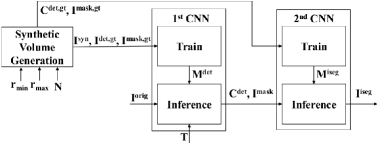
Figure 1: Block diagram of the proposed method

Figure 1 is a block diagram of our proposed method for 3D nuclei instance segmentation. A 3D image volume of size $X\times Y\times Z$ is denoted as $I$ and the $p^{\text{th}}$ 2D focal plane image of size $X\times Y$ along the $z$-direction is denoted as $I_{z_{p}}$, where $p\in\{1,\dots,Z\}$. A subvolume of $I$, whose $x$-coordinate is $q_{i}\leq x\leq q_{f}$, $y$-coordinate is $r_{i}\leq y\leq r_{f}$, $z$-coordinate is $p_{i}\leq z\leq p_{f}$ is denoted as $I_{\left(q_{i}:q_{f},r_{i}:r_{f},p_{i}:p_{f}\right)}$, where $q_{i}\in\{1,\dots,X\}$, $q_{f}\in\{1,\dots,X\}$, $r_{i}\in\{1,\dots,Y\}$, $r_{f}\in\{1,\dots,Y\}$, $p_{i}\in\{1,\dots,Z\}$, and $p_{f}\in\{1,\dots,Z\}$. It is required that $q_{i}\leq q_{f}$, $r_{i}\leq r_{f}$, and $p_{i}\leq p_{f}$. Lastly, a voxel is denoted as v.

Our method consists of two CNNs as shown in Figure 1. The first CNN, $M^{det}$, is used for nuclei detection and binary segmentation and the second CNN, $M^{iseg}$, is used for nuclei instance segmentation. To segment each nucleus using the second CNN, the first CNN produces a set of coordinates of the nuclei center locations, denoted as $C^{det}$, and a nuclei mask volume denoted as $I^{mask}$. Specifically, $C^{det}$ consists of the centroid coordinates of components in a detection volume, $I^{det}$. To accurately select the elements of $C^{det}$, especially when multiple nuclei are touching, the components in $I^{det}$ are chosen to have no touching regions for distinct nuclei. The second CNN segments an individual nucleus in a 3D patch from $I^{mask}$ centered at $C^{det}$ and is color-coded to produce the final segmentation volume, $I^{iseg}$. Note that color-coding is done to visually label each nucleus in $I^{iseg}$. To train the two CNNs a SpCycleGAN described in [18] is used to generate synthetic microscopy volumes, $I^{syn}$. Our implementation is done using PyTorch [19].

II-A Synthetic Volume Generation

As indicated above, creating labeled ground truth 3D volumes is tedious. We use the SpCycleGAN we described in [18] to produce synthetic microscopy 3D volumes that we use for training. Note we do not need any actual ground truth volumes to use the approach described in this section. Synthetic microscopy volumes, $I^{syn}$, nuclei mask ground truth volumes, $I^{mask,gt}$, and detection ground truth volumes, $I^{det,gt}$, need to be generated. We start by generating a random 3D nuclei mask volume and then use it to generate the synthetic volume. To generate $I^{mask,gt}$ we develop two approaches: the first approach produces $N$ synthetic spherical nuclei and the second approach produces elliptical nuclei based on nuclei structures in $I^{orig}$. For the first approach the $i^{\text{th}}$ synthetic nuclei, $I^{mask,i}$, is generated as a sphere with a randomly selected radius, $r_{i}$, between $r_{min}$ and $r_{max}$, and centered at a randomly selected coordinate, $C^{det,i}$, where $1\leq i\leq N$. Simultaneously, the $i^{\text{th}}$ central region, $I^{det,i}$, is generated where a central region of a nucleus is defined as a sphere inside the nucleus where the centroid of the central region matches to the centroid of the nucleus. We intentionally set the radius of $I^{det,i}$ to be $\frac{r_{i}}{2}$ to avoid multiple connected central regions although their corresponding synthetic nuclei may be touching. Once $N$ synthetic nuclei and their central regions are produced, they are added to $I^{mask,gt}$ and $I^{det,gt}$ sequentially where $I^{mask,gt}$ and $I^{det,gt}$ are initialized to zero. If $I^{mask,i}$ overlaps with any previous synthetic nuclei in $I^{mask,gt}$, then $I^{mask,i}$ and $I^{det,i}$ are not added to $I^{mask,gt}$ and $I^{det,gt}$, respectively.

For the second approach $I^{mask,i}$ is generated as an ellipsoid with randomly and independently selected three semi-axes between $r_{min}$ and $r_{max}$, randomly rotated in $x$, $y$, and $z$-axes, and centered at a randomly selected coordinate, $C^{det,i}$. In our experiments we used both approaches for generating synthetic images.

Once the nuclei mask ground truth volume, $I^{mask,gt}$, and the detection ground truth volume, $I^{det,gt}$, are generated, we use the SpCycleGAN to generate the corresponding synthetic volume, $I^{syn}$. For our experiments we generated 20 sets of synthetic volumes with a size of $128\times 128\times 128$. Figure 2 shows examples of a real microscopy volume, a synthetic microscopy volume, and synthetic ground truth volumes visualized by Voxx [20], respectively.

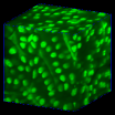
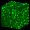
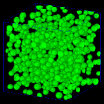
Figure 2: Example volumes (a) real microscopy volume (b) synthetic microscopy volume (c) nuclei mask ground truth volume (d) detection ground truth volume

II-B Nuclei Detection and Binary Segmentation

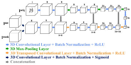
Figure 3: Our first CNN architecture (see Figure 1)

Our first CNN used for nuclei detection and binary segmentation outputs nuclei center locations, $C^{det}$, and a nuclei mask volume, $I^{mask}$ (Figure 1). This CNN is shown in more detail in Figure 3 and uses a modified 3D U-Net architecture [13]. $C^{det}$ can be selected by finding centroids of elements of $I^{det}$. To avoid false-detection, labels in $I^{det}$ are labeled as background if $I^{mask}$ at the same voxel locations are labeled as background. Also, components with the number of voxels less than $T$ are not considered in order to remove noise. A 3D convolutional layer consists of a convolutional operation with a $3\times 3\times 3$ kernel with 1 voxel padding, 3D batch normalization, and a rectified-linear unit (ReLU) activation function. Note that the Sigmoid function is used as an activation function for the last convolutional layers. In the encoder, 3D max-pooling layer uses $2\times 2\times 2$ window with a stride of 2. In the decoder, a 3D transposed convolutional layer followed by 3D batch normalization and a ReLU activation function is used. In addition, concatenation transfers feature maps from the encoder to the decoder. The size of input/output volumes are $64\times 64\times 64$. If the size of $I^{orig}$ is larger than $64\times 64\times 64$, then a 3D window with size of $64\times 64\times 64$ is moved in the $x$, $y$, and $z$-directions until the entire $I^{orig}$ is processed [14]. During training, the Adam optimizer [21] is used with a learning rate of 0.001. The training loss function is a sum of the Binary Cross Entropy (BCE) loss of the detection volume and the BCE loss of the nuclei mask volume. The BCE loss, $L^{BCE}$, is defined as $L^{BCE}(I^{out},I^{gt})=-\frac{1}{V}\sum_{\textbf{v}=1}^{V}\big{(}I^{gt}(\textbf{v})\log I^{out}(\textbf{v})+(1-I^{gt}(\textbf{v}))\log(1-I^{out}(\textbf{v}))\big{)}$ where $I^{out}$ is the output volume, $I^{gt}$ is the ground truth volume, and $V$ is the total number of voxels in the volume. For the training set, we used 160 synthetic volumes with a size of $64\times 64\times 64$. Each synthetic volume with a size of $128\times 128\times 128$ generated in the synthetic volume generation stage is divided into 8 volumes with a size of $64\times 64\times 64$.

II-C Nuclei Instance Segmentation

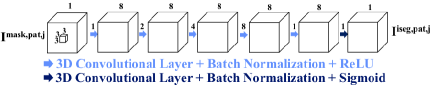
Figure 4: Our second CNN architecture (see Figure 1)

The goal of our method is nuclei instance segmentation which is segmenting individual detected nuclei with distinct labels. Therefore, the last step is to segment each nucleus in $I^{mask}$ at a detected coordinate, $C^{det}$, using our second CNN shown in Figure 4. First, the $j^{\text{th}}$ nucleus is cropped and included in a 3D patch with a size of $32\times 32\times 32$ from $I^{mask}$ centered at $C^{det,j}$, denoted as $I^{mask,pat,j}$. Then the second CNN segments only the $j^{\text{th}}$ nucleus in $I^{mask,pat,j}$ and removes other nuclei structures partially included in the patch. Here, we denote the segmented nucleus as $I^{iseg,pat,j}$. Once the $j^{\text{th}}$ nucleus is segmented, it is color-coded and inserted in $I^{iseg}$ where the center location of $I^{iseg,pat,j}$ lies at $C^{det,j}$.

The second CNN in Figure 1, $M^{iseg}$, consists of a series of 3D convolutional layers. We use dilated convolutions [22] to have receptive field larger than the size of the patch. From the $k^{\text{th}}$ feature map, $I^{k}$, with a convolution filter, $h$, the $(k+1)^{\text{th}}$ feature map, $I^{k+1}$, is generated using a $d$-dilated convolution at a voxel v as $I^{k+1}(\textbf{v})=\sum_{\textbf{u}}I^{k}(\textbf{v}-d\textbf{u})h(\textbf{u})$ where $d$ is known as the dilation factor. Figure 4 shows the dilation factors for the convolutional layers such that the final receptive field is larger than $32\times 32\times 32$. Note the kernel size for the last convolutional layer of the second CNN is $1\times 1\times 1$. During training, the Adam optimizer [21] is used with a learning rate of 0.001. The BCE loss is used as the training loss function. 300 patches from $I^{mask,gt}$ centered at $C^{det,gt}$ are used for the training.

III Experimental Results

Our method is tested on three rat kidney data sets. All data sets consist of gray scale images of size $X=512\times Y=512$. Data-I consists of $Z=512$ images, Data-II of $Z=415$, and Data-III of $Z=45$. To match resolution in $z$-direction to resolution in $x$ and $y$-directions, Data-II is downsampled in $z$-direction by a factor of 2 and Data-III is linearly interpolated in $z$-direction by a factor of 2. $r_{min}=4$, $r_{max}=6$, and $N=1000$ with a spherical model and $T=10$ for Data-I, $r_{min}=6$, $r_{max}=9$, and $N=200$ with an ellipsoidal model and $T=20$ for Data-II, and $r_{min}=6$, $r_{max}=9$, and $N=50$ with a spherical model and $T=30$ for Data-III are used, respectively. Note that the size of synthetic nuclei for Data-I is small, so the size of patches during nuclei instance segmentation is reduced to $16\times 16\times 16$ and the fourth convolutional layer in $M^{iseg}$ is removed. Figure 5 shows original images and segmented images for Data-I, Data-II, and Data-III.

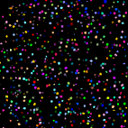
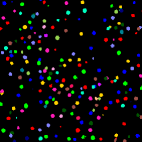
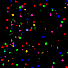
Figure 5: Original and segmented images in Data-I, Data-II, and Data-III (a) $I^{orig}_{z_{97}}$ for Data-I, (b) $I^{orig}_{z_{403}}$ for Data-II, (c) $I^{orig}_{z_{14}}$ for Data-III, (d) $I^{iseg}_{z_{97}}$ for Data-I, (e) $I^{iseg}_{z_{403}}$ for Data-II, (f) $I^{iseg}_{z_{14}}$ for Data-III

Our method was compared to other segmentation methods using object-wise evaluation criterion [23]. The other segmentation methods include Squassh [7], watershed [3], our previous detection and segmentation method [15] that we will denote as Purdue1, and our previous segmentation method using a SpCycleGAN [18] that we will denote as Purdue2. Note our method in [18] generates binary segmentation masks but cannot label nuclei distinctly. To label touching nuclei distinctly, we added a post-processing step in Purdue2 using morphological operations with a 3D erosion, a 3D connected component for color-coding, and a 3D dilation with a sphere of radius of 1 used as the structuring element. For the object-wise evaluation, Precision ($P$), Recall ($R$), and F1 score ($F1$) are defined as $P=\frac{N_{TP}}{N_{TP}+N_{FP}}$, $R=\frac{N_{TP}}{N_{TP}+N_{FN}}$, and $F1=\frac{2PR}{P+R}$, where $N_{TP}$, $N_{FP}$, and $N_{FN}$ are the number of true positive objects, the number of false positive objects, and the number of false negative objects, respectively. A segmented nucleus is defined as a true positive object if it intersects at least 50% of the corresponding ground truth nucleus. Otherwise, it is defined as a false positive object. A ground truth nucleus is defined as a false negative object if it intersects less than 50% of the corresponding segmented nucleus or there is no corresponding segmented nucleus. In our evaluation, we generated a 3D ground truth volume, $I^{gt}_{\left(193:320,193:320,31:94\right)}$, using ITK-SNAP [24] from Data-I with size of $128\times 128\times 64$ containing 283 nuclei. Note that any components whose number of voxels is less than 50 are removed on $I^{iseg}_{\left(193:320,193:320,31:94\right)}$ and $I^{gt}_{\left(193:320,193:320,31:94\right)}$ to remove partially included nuclei on the boundary of the subvolume.

Table I and Figure 6 show the object-based evaluation and the segmentation results visualized by Voxx [20] of other methods and our new proposed method for Data-I, respectively. Squassh [7] cannot distinguish nuclei and non-nuclei structures and cannot successfully separate touching objects. For watershed [3], $I^{orig}$ is first binarized by a manually-selected threshold value of 64. Thresholding cannot distinguish nuclei and non-nuclei structures and watershed technique over-segments foreground region. Purdue1 can reject non-nuclei structures but still have a poor F1 score. Purdue2 can generate an accurate binary segmentation mask but cannot separate all touching nuclei. Our proposed method, detecting the locations of nuclei and individually segmenting nuclei in 3D patches using the SpCycleGAN, can successfully segment and separate nuclei.

TABLE I: Object-wise evaluation for various methods for Data-I

	Precision	Recall	F1 score
Squassh [7]	85.07%	20.14%	32.57%
Watershed [3]	51.14%	92.13%	65.78%
Purdue1 [15]	68.35%	90.22%	77.78%
Purdue2 [18]	91.20%	82.01%	86.36%
Proposed Method	93.47%	96.80%	95.10%

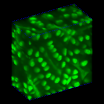
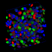
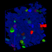
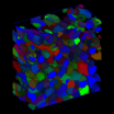
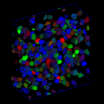
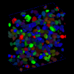
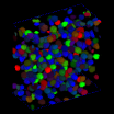
Figure 6: Comparison of other segmentation methods and our proposed method of Data-I (a) original volume, (b) ground truth volume, (c) Squassh, (d) Watershed, (e) Purdue1, (f) Purdue2, (g) our proposed method

IV Conclusions

This paper presented a nuclei instance segmentation method using a center-extraction technique to detect the center locations of nuclei. We individually segmented nuclei in 3D patches surrounding the nuclei. Our method can successfully segment nuclei visually and numerically. In the future we plan to develop a synthetic volume generation model which can produce synthetic nuclei with other shapes.

References

- [1] K.W. Dunn, R.M. Sandoval, K.J. Kelly, P.C. Dagher, G.A. Tanner, S.J. Atkinson, R.L. Bacallao, and B.A. Molitoris, “Functional studies of the kidney of living animals using multicolor two-photon microscopy,” American Journal of Physiology-Cell Physiology, vol. 283, no. 3, pp. C905–C916, September 2002.
- [2] C. Vonesch, F. Aguet, J. Vonesch, and M. Unser, “The colored revolution of bioimaging,” IEEE Signal Processing Magazine, vol. 23, no. 3, pp. 20–31, May 2006.
- [3] L. Vincent and P. Soille, “Watersheds in digital spaces: an efficient algorithm based on immersion simulations,” IEEE Transactions on Pattern Analysis and Machine Intelligence, vol. 13, no. 6, pp. 583–598, June 1991.
- [4] X. Yang, H. Li, and X. Zhou, “Nuclei segmentation using marker-controlled watershed, tracking using mean-shift, and Kalman filter in time-lapse microscopy,” IEEE Transactions on Circuits and Systems I: Regular Papers, vol. 53, no. 11, pp. 2405–2414, November 2006.
- [5] R. Delgado-Gonzalo, V. Uhlmann, D. Schmitter, and M. Unser, “Snakes on a plane: A perfect snap for bioimage analysis,” IEEE Signal Processing Magazine, vol. 32, no. 1, pp. 41–48, January 2015.
- [6] A. Dufour, V. Shinin, S. Tajbakhsh, N. Guillen-Aghion, J.C. Olivo-Marin, and C. Zimmer, “Segmenting and tracking fluorescent cells in dynamic 3-D microscopy with coupled active surfaces,” IEEE Transactions on Image Processing, vol. 14, no. 9, pp. 1396–1410, September 2005.
- [7] A. Rizk, G. Paul, P. Incardona, M. Bugarski, M. Mansouri, A. Niemann, U. Ziegler, P. Berger, and I.F. Sbalzarini, “Segmentation and quantification of subcellular structures in fluorescence microscopy images using Squassh,” Nature Protocols, vol. 9, no. 3, pp. 586–596, February 2014.
- [8] Y. LeCun, Y. Bengio, and G. Hinton, “Deep learning,” Nature, vol. 521, pp. 436–444, May 2015.
- [9] G. Litjens, T. Kooi, B.E. Bejnordi, A.A.A. Setio, F. Ciompi, M. Ghafoorian, J.A.W.M. van der Laak, B. van Ginneken, and C.I. Sanchez, “A survey on deep learning in medical image analysis,” Medical Image Analysis, vol. 42, pp. 60–88, July 2017.
- [10] H. Chen, X. Qi, L. Yu, and P.-A. Heng, “DCAN: Deep contour-aware networks for accurate gland segmentation,” Proceedings of the IEEE Conference on Computer Vision and Pattern Recognition, pp. 2487–2496, June 2016, Las Vegas, NV.
- [11] S. Graham and N.M. Rajpoot, “SAMS-NET: Stain-aware multi-scale network for instance-based nuclei segmentation in histology images,” Proceedings of the IEEE International Symposium on Biomedical Imaging, pp. 590–594, April 2018, Washington, D.C.
- [12] T. Falk, D. Mai, R. Bensch, O. Cicek, A. Abdulkadir, Y. Marrakchi, A. Bohm, J. Deubner, Z. Jackel, K. Seiwald, A. Dovzhenko, O. Tietz, C. Dal Bosco, S. Walsh, D. Saltukoglu, T.L. Tay, M. Prinz, K. Palme, M. Simons, I. Diester, T. Brox, and O. Ronneberger, “U-Net: deep learning for cell counting, detection, and morphometry,” Nature Method, vol. 16, pp. 67–70, January 2019.
- [13] O. Cicek, A. Abdulkadir, S.S. Lienkamp, T. Brox, and O. Ronneberger, “3D U-Net: Learning dense volumetric segmentation from sparse annotation,” Proceedings of the Medical Image Computing and Computer-Assisted Intervention, pp. 424–432, October 2016, Athens, Greece.
- [14] D.J. Ho, C. Fu, P. Salama, K.W. Dunn, and E.J. Delp, “Nuclei segmentation of fluorescence microscopy images using three dimensional convolutional neural networks,” Proceedings of the Computer Vision for Microscopy Image Analysis workshop at Computer Vision and Pattern Recognition, pp. 834–842, July 2017, Honolulu, HI.
- [15] D.J. Ho, C. Fu, P. Salama, K.W. Dunn, and E.J. Delp, “Nuclei detection and segmentation of fluorescence microscopy images using three dimensional convolutional neural networks,” Proceedings of the IEEE International Symposium on Biomedical Imaging, pp. 418–422, April 2018, Washington, D.C.
- [16] I. Goodfellow, J. Pouget-Abadie, M. Mirza, B. Xu, D. Warde-Farley, S. Ozair, A. Courville, and Y. Bengio, “Generative adversarial nets,” Proceedings of the Advances in Neural Information Processing Systems, pp. 2672–2680, December 2014, Montreal, Canada.
- [17] J.Y. Zhu, T. Park, P. Isola, and A.A. Efros, “Unpaired image-to-image translation using cycle-consistent adversarial networks,” Proceedings of the IEEE International Conference on Computer Vision, pp. 2223–2232, October 2017, Venice, Italy.
- [18] C. Fu, S. Lee, D.J. Ho, S. Han, P. Salama, K.W. Dunn, and E.J. Delp, “Three dimensional fluorescence microscopy image synthesis and segmentation,” Proceedings of the Computer Vision for Microscopy Image Analysis workshop at Computer Vision and Pattern Recognition, pp. 2302–2310, June 2018, Salt Lake City, UT.
- [19] A. Paszke, S. Gross, S. Chintala, G. Chanan, E. Yang, Z. DeVito, Z. Lin, A. Desmaison, L. Antiga, and A. Lerer, “Automatic differentiation in pytorch,” Proceedings of the Autodiff Workshop at the Advances in Neural Information Processing Systems, pp. 1–4, December 2017, Long Beach, CA.
- [20] J.L. Clendenon, C.L. Phillips, R.M. Sandoval, S. Fang, and K.W. Dunn, “Voxx: a PC-based, near real-time volume rendering system for biological microscopy,” American Journal of Physiology-Cell Physiology, vol. 282, no. 1, pp. C213–C218, January 2002.
- [21] D.P. Kingma and J. Ba, “Adam: A method for stochastic optimization,” arXiv preprint arXiv:1412.6980, pp. 1–15, December 2014.
- [22] F. Yu and V. Koltun, “Multi-scale context aggregation by dilated convolutions,” arXiv preprint arXiv:1511.07122, pp. 1–13, April 2016.
- [23] D.M.W. Powers, “Evaluation: from Precision, Recall and F-measure to ROC, Informedness, Markedness and Correlation,” Journal of Machine Learning Technologies, vol. 2, no. 1, pp. 37–63, December 2011.
- [24] P.A. Yushkevich, J. Piven, H.C. Hazlett, R.G. Smith, S. Ho, J.C. Gee, and G. Gerig, “User-guided 3D active contour segmentation of anatomical structures: Significantly improved efficiency and reliability,” NeuroImage, vol. 31, no. 3, pp. 1116–1128, July 2006.