Bayesian optimization of a free-electron laser
Abstract
The Linac Coherent Light Source changes configurations multiple times per day, necessitating fast tuning strategies to reduce setup time for successive experiments. To this end, we employ a Bayesian approach to transport optics tuning to optimize groups of quadrupole magnets. We use a Gaussian process to provide a probabilistic model of the machine response with respect to control parameters from a modest number of samples. Subsequent samples are selected during optimization using a statistical test combining the model prediction and uncertainty. The model parameters are fit from archived scans, and correlations between devices are added from a simple beam transport model. The result is a sample-efficient optimization routine, which we show significantly outperforms existing optimizers.
Modern large-scale scientific experiments can have complicated operational requirements with performance degraded by errors in controls and dependencies on drifting or random variables. A prime example of this is the Linac Coherent Light Source (LCLS) emma:lcls , an x-ray free electron laser (FEL) user facility that supports a wide array of scientific experiments. At LCLS, skilled human operators tune dozens of control parameters on-the-fly to achieve custom photon beam characteristics, and this process cuts into valuable time allocated for each user experiment. Model-independent optimizers can help automate tuning, with successful demonstrations using simplex simplex ; tomin:ocelot , extremum seeking ES ; es_rf_tuning_paper , and robust conjugate direction search rcds ; rcds_demo . However, these methods require a large number of expensive acquisitions and can become stuck in local optima. To improve the efficiency of optimization beyond these methods, a model of the system is necessary good_regulator ; in this work, we use Bayesian optimization with Gaussian process (GP) models during live tuning of LCLS. First, we use archived data to estimate the length scales of tuning parameters in the model. Second, we show that adding physics-inspired correlations between parameters further speeds convergence. Finally, we discuss possible directions for improvement.
Bayesian optimization is a sample efficient and gradient-free approach to global optimization of black-box functions with noisy outputs mockus1975 ; freitas:bayes_opt_review ; freitas:tutorial . This efficiency comes from application of Bayes theorem to incorporate prior knowledge and previous steps to maximize the value of each new measurement. Numerical optimization of an acquisition function, incorporating the model’s expectation and uncertainty, guides the selection of each new point to sample, giving Bayesian optimization the advantage of balancing exploration with exploitation. Prior knowledge can improve the efficiency of the optimization and constrain the search in low signal-to-noise states. Bayesian optimization has been applied to a fast growing number of domains; for example, resource prospecting kriging:origins ; kriging:water , active policy search for reinforcement learning bayes-policy-search , hyper parameter tuning bayes-hyperparam-tuning , experimental control yager2019 etc.
Bayesian optimization requires a probabilistic model providing estimates and uncertainties of a target or objective function. A Gaussian process (GP) is a popular choice as it is a non-parametric regressor which calculates probability densities over a space of functions rw:gpml_book . Whereas a Gaussian distribution is characterized by a mean and covariance , a Gaussian process is determined by mean and covariance functions: , where are possible inputs to the objective. The mean is a predetermined function encoding prior understanding of the objective. This mean could be a fit to data but is typically set to zero. The covariance, or kernel, function describes the similarity between pairs of points and . As a non-parametric model, a GP is constructed directly from the training instances themselves, allowing the model complexity to grow with observations and adapt to previously unexplored regions of the feature space. There are many Gaussian process codes available GPy ; GPFlow ; GPML ; PyMC3 , and many of these packages employ various techniques to limit computation times for large data sets. In our case, we use an online GP model mitch:spwogp interfaced to LCLS via the Ocelot optimization framework tomin:ocelot . The online model saves frequent computations to speed subsequent predictions.
In this Letter we apply Gaussian process optimization to the problem of maximizing the LCLS x-ray FEL pulse energy. The FEL instability is a collective effect so performance depends strongly on the current density and therefore beam size. A strong focusing quadrupole magnet system maintains a small beam size to maximize the pulse energy produced. The FEL pulse energy is therefore a function of quadrupole magnet strengths (field integral in kiloGauss, kG) and the input electron beam parameters. Since these beam parameters drift throughout the day and are generally hard to measure, LCLS operators perform tuning scans to optimize the quadrupole strengths many times per day.
We model the FEL dependence on quadrupoles with a Gaussian process surrogate. Prior information guides the selection of the kernel and its hyperparameters. We approach this process in two ways: first, from an intuitive view of basis functions, and second in a principled way using Bayesian model selection. An attractive feature of Gaussian process modeling is the interpretability of the kernel’s functional form. The prediction can be viewed as a convolution of measured data with a kernel function response to measured data points (analogous to a Green’s function approach); thus, kernel functions should be derived from basis functions that look like the system being modeled. We exploit this insight here, explaining the interpretation of each kernel hyperparameter, and then show that the basis function approach also maximizes the GP marginal likelihood.
Motivated by the observation that the FEL pulse energy response to quadrupole magnets looks bell-shaped, we choose the popular radial basis function (RBF) kernel, . Here, is the covariance function amplitude and is a diagonal matrix of inverse square length scales. This kernel encodes the expectation that for smooth functions, nearby pairs of points are more similar than distant points. The length scales set the distance over which the function changes in each dimension. The amplitude parameter captures the variance of the target function values with respect to variations in the inputs and therefore determines the prior prediction uncertainty far from any sampled points. Functions which are less smooth may be better modeled by the Matern kernel, whereas periodic functions are best treated with a periodic kernel. Kernels may be added or multiplied together to yield new, more expressive kernels duvenaud:kernel_composition ; sun:nkn and neural network warping functions may be applied to the inputs before passing to a kernel manifoldgp ; wilson:dkl . Modeling noisy targets can be achieved by adding a Gaussian noise kernel , where is the noise variance parameter, and is the Dirac delta function. The noise parameter models the variance of the prediction at a sampled point.
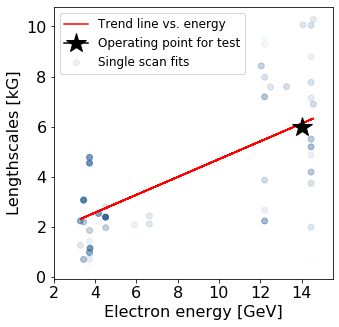
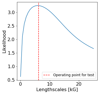

The RBF length scales depend on the electron beam energy because the focusing strength of a quadrupole magnet depends on the ratio of the electron energy to the magnetic field strength (i.e. the rigidity). Moreover, the beamsize response varies between each quadrupole even at a single energy. We therefore determine RBF length scales for each quadrupole independently as a function of electron beam energy. We first approach the estimation of these length scales with 1D Gaussian fits to historical tuning scans. The black star in Fig. 1(a) shows the average of many such fit lengths to scans with electron beam energies near 14 GeV for a particular quadrupole. We also estimate the RBF length scales from maximization of the marginal likelihoods of GP fits to the archive data. An example of this procedure for a scan at 14 GeV is shown in Fig. 1(b), where we can see that 50% deviations from the optimal length scale decreases the marginal likelihood by merely 10%–providing some tolerance to errors in the parameter determination. Figure 1(a) shows the maximum likelihood length scales for various scans as a function of electron beam energy. The red line is a linear fit to the length scales with points weighted by widths of the marginal likelihoods (effectively the credibilities) for each individual point estimate. The resulting trend is then used to construct RBF kernels for optimization, and we observe reasonable agreement with our length scale estimate from the Gaussian fits. We repeat this procedure to determine length scale trends as a function of electron energy for each quadrupole.
Online optimization proceeds by first measuring the initial state of the machine and then initializing the Gaussian process model with the appropriate kernel and first measured point. The GP provides a probabilistic surrogate model for the machine, and an upper confidence bound (UCB) acquisition function ucb is constructed from the GP prediction mean and variance. The point maximizing the UCB function is chosen as the next measurement which is then acquired and added to the GP, finishing one step through the optimization process. The optimization continues in this way until reaching a time limit or a target performance.
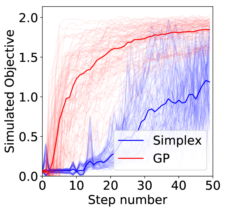
Figure 1(c) shows results from live optimization of the FEL pulse energy simultaneously on 12 quadrupoles. In this example, Bayesian optimization (red curves) is approximately 4 times faster than the standard Nelder-Mead simplex algorithm (blue curves), and reaches a higher optimum. The different lines for each algorithm correspond to scans with identical starting conditions.
We also compare simplex and Bayesian optimization in a simulation environment. Ideally we would use physics codes such as elegant elegant and Genesis Genesis to model the transport and FEL behavior, however due to mismatch between the codes and measured performance, as well as computational expense for each simulation, we instead fit a beam transport model as described below. Though the beam transport model does not capture the full complexity of the real machine, it allows us to compare the relative performance of simplex and Bayesian optimization with a simulated objective function, which we find consistent with live scans (Fig. 1(d)).
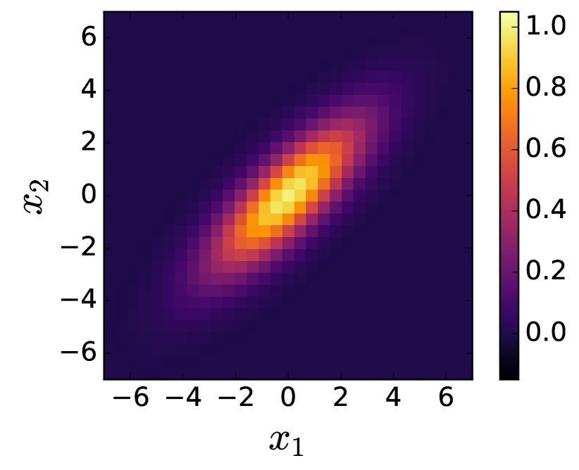
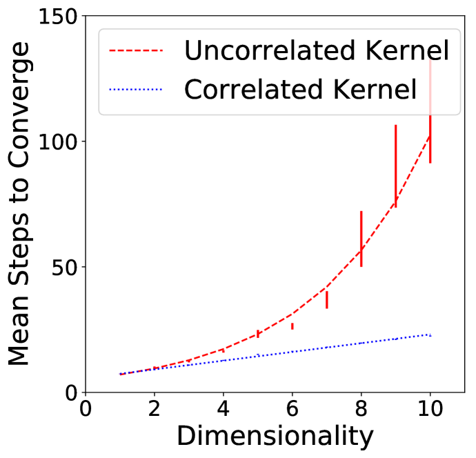
Correlated kernels become advantageous when a system’s response is to one input depends strongly on one or more of the other inputs as in Figure 2(a). Figure 2(b) shows a GP regression on noisy samples (RMS noise is 10% of the signal peak) from a correlated ground truth (Fig. 2(a)) with an isotropic kernel, while Figure 2(c) shows a GP regression on the same samples but with a kernel sharing the same correlation as the ground truth (). The latter model is more representative of the system. To demonstrate the effectiveness of a correlated model for regulating the system, we perform Bayesian optimization with and without kernel correlations for various dimensional spaces with nearest-neighbor correlation coefficients of . Each point in Figure 2(d) shows the average number of steps to achieve of the ground truth peak amplitude for 100 runs starting at a random position such that the starting signal-to-noise ratio is unity. The relative efficiency of the correlated kernel grows exponentially with the number of dimensions, making it attractive for high-dimensional optimization at accelerators.


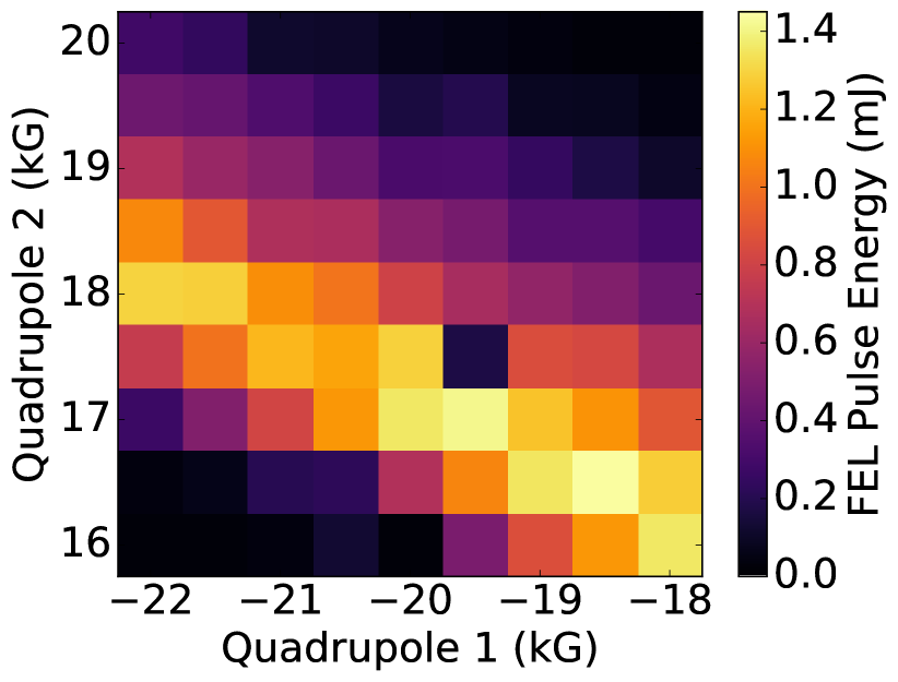
FEL quadrupole optimization is an example of a highly correlated system. Strong focusing in charged particle transport relies on a series of oppositely polarized quadrupole fields wiedemann . Each quadrupole focuses in one transverse plane while defocusing in the orthogonal plane, and repeated application of alternate focusing/defocusing results in net focusing in both planes. Increasing the strength of one quadrupole field necessitates increasing the strength of the next quadrupole (with opposite sign) to achieve net focusing, resulting in negative correlations between nearby focusing elements. Figure 3(a) shows the average FEL pulse energy response to variation of two adjacent quadrupoles in a matching section just upstream of the FEL undulator magnets. Similar correlations exist between all pairs of quadrupoles.
Ideally we would calculate correlations from maximum likelihood fits to the archive data, as done for the length scales. However, due to sparsity in the sampled data, we instead calculate correlations from a beam physics transport model. The FEL pulse energy (denoted as ) is a correlation-preserving function of the transverse area of the beam, , averaged along the interaction, with . zhirong:fel_book . As a consequence, any correlated response of the quadrupole magnets with respect to beam size preserves correlations with respect to the FEL energy.
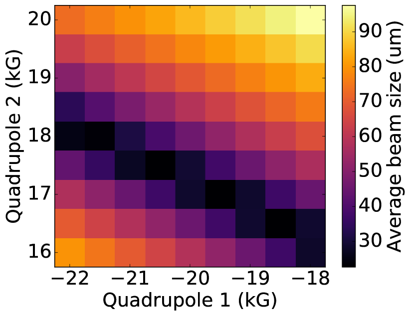

To model the average beam size in the undulator line as a function of quadrupole magnets, we estimate the Twiss, or focusing, parameters of the electron beam. Realistic Twiss parameters may be inferred from measurements of the beam size throughout a drift or in response to varying focusing emittance_measurements . Alternatively, we can use the premise that maximized FEL performance implies approximately matched Twiss parameters in the undulator line. Starting from these initial conditions, we then use linear transport matrices calculated from live quadrupole values wiedemann to calculate the beam’s size along the undulator for any arbitrary deviation in quadrupole strength. The result shown in Figure 3(b) is a modeled beam size that matches the correlation to the FEL pulse energy (Fig. 3(a)).
To find correlations from the beam physics model, we approximate the beam size about the match by the Hessian , where and iterate over all pairs of quadrupoles. Correlations are extracted by identifying the diagonal elements as the functional curvature along each slice and factoring these out of the Hessian .
We now need to combine the correlations with the length scales in the RBF kernel. In principle, the Hessian can also be used to calculate the length scales. However, the post-saturation FEL process is computationally expensive to model and further complicated by leaked dispersion and orbit jitter so characteristic length scales are difficult to compute on the fly. As a result, we combine the modeled correlations with length scales measured from fits to archive data as described earlier. A diagonal matrix of inverse slice lengths determined from archived scans are combined with the precision matrix in the kernel, , to yield a kernel with slice lengths from archived scans and correlations from the simulated beam transport model. With a more sophisticated model that incorporates a wider range of effects, it should be possible to train hyperparameters entirely from simulations.
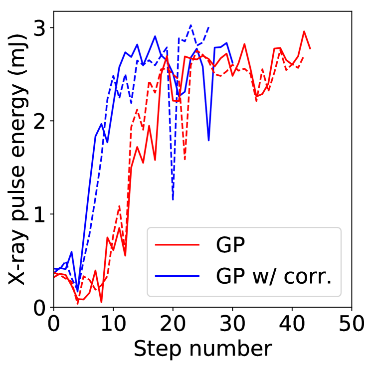
We tested optimization with GPs built with and without correlations for four adjacent matching quadrupole magnets located in the transport between the accelerator and the FEL undulators. The results, presented in Figure 3(c), show that the correlated GP model outperforms the uncorrelated GP. Furthermore, we find consistency of these results with simulations based on correlations from the beam transport model as shown in Figure 3(d). It is interesting to note that the Bayesian optimizer maximized the FEL with a similar number of steps for the 12 quadrupole case (Fig. 1(c)), seemingly in contradiction to Figure 2(d). The similarity is due to the fact that to leading order (assuming a monoenergetic beam and linear optics), only four quadrupole magnets are needed to match the four Twiss parameters into the undulator line. However, optimizing more quadrupoles further increases the FEL pulse energy by reducing chromatic effects which suppress FEL gain by increasing the electron beam emittance. While four quadrupoles can recover a significant fraction of peak performance, in practice operators typically cycle through subsets of all of the controllable quadrupoles. With the ever increasing number of input dimensions or controls, the GP with correlations is expected to perform exponentially faster than without.
In this letter we showed that online Bayesian optimization with length scales estimated from archived historical data can tune the LCLS FEL pulse energy more efficiently than the current state-of-the-art Nelder-Mead simplex algorithm. Moreover, we showed that adding physics-informed correlations, trained from beam optics models, further improves tuning efficiency. The latter effect was demonstrated with four control parameters, and the improvement is expected to grow dramatically as the number of dimensions increases when controlling more variables such as RF variables or undulator strengths. The flexibility of the GP enables training from archived data, simulations, and physical models.
We expect Bayesian optimization will become a standard tuning method for LCLS-II. Future improvements will further improve efficiency and operational ability. This Letter focused on the most time-consuming task of tuning quadrupoles, but we expect additional applications to other accelerator and beamline tasks, e.g. reducing bandwidth, optimizing taper juhao:taperopt , focusing and alignment, etc. Adding ‘safety’ constraints to the acquisition function can guide the exploration while ensuring operational requirements are met (for instance, avoiding transient drops in FEL pulse energy or keeping losses low) kirschner:swissfel . More expressive GPs, for example deep kernel learning DKL or deep GPs Deep-GP can learn more complicated functions and extract additional value from historical data. In our example, we exploited the physics of strong focusing to learn correlations between parameters. Physics abounds with well verified mathematical models and incorporating additional physics knowledge into the prior, either explicitly in the formulation of the kernel function or via additional training with simulation can have a dramatic effect on optimization efficiency.
Acknowledgements.
The authors are grateful to Hugo Slepicka and Sergey Tomin for their help with the details of the Ocelot-optimizer code and to Hugo Slepicka and Ahmed Osman for adding helpful LCLS-specific functions to Ocelot-optimizer. This work was supported by the Department of Energy, Laboratory Directed Research and Development program at SLAC National Accelerator Laboratory, under contract DE-AC02-76SF00515.References
- (1) P. Emma, R. Akre, J. Arthur, R. Bionta, C. Bostedt, J. Bozek, A. Brachmann, P. Bucksbaum, R. Coffee, F. J. Decker, Y. Ding, D. Dowell, S. Edstrom, A. Fisher, J. Frisch, S. Gilevich, J. Hastings, G. Hays, Ph Hering, Z. Huang, R. Iverson, H. Loos, M. Messerschmidt, A. Miahnahri, S. Moeller, H. D. Nuhn, G. Pile, D. Ratner, J. Rzepiela, D. Schultz, T. Smith, P. Stefan, H. Tompkins, J. Turner, J. Welch, W. White, J. Wu, G. Yocky, and J. Galayda. First lasing and operation of an ångstrom-wavelength free-electron laser. Nature Photonics, 4(9):641–647, 9 2010.
- (2) J. A. Nelder and R. Mead. A Simplex Method for Function Minimization. The Computer Journal, 7(4):308–313, 1 1965.
- (3) S. Tomin, G. Geloni, I. Agapov, I. Zagorodnov, Ye. Fomin, Yu. Krylov, A. Valintinov, W. Colocho, T.M. Cope, A. Egger, and D. Ratner. Progress in automatic software-based optimization of accelerator performance. In IPAC 2016 - Proceedings of the 7th International Particle Accelerator Conference, 2016.
- (4) Alexander Scheinker, Xiaoying Pang, and Larry Rybarcyk. Model-independent particle accelerator tuning. Physical Review Special Topics - Accelerators and Beams, 16(10):102803, 10 2013.
- (5) Alexander Scheinker, Xiaobiao Huang, and Juhao Wu. Minimization of Betatron Oscillations of Electron Beam Injected Into a Time-Varying Lattice via Extremum Seeking. IEEE Transactions on Control Systems Technology, 26(1):336–343, 1 2018.
- (6) Xiaobiao Huang. Robust simplex algorithm for online optimization. Physical Review Accelerators and Beams, 21(10):104601, 10 2018.
- (7) Xiaobiao Huang and James Safranek. Online optimization of storage ring nonlinear beam dynamics. Physical Review Special Topics - Accelerators and Beams, 18(8), 2015.
- (8) Roger C. Conant and W. Ross Ashby. Every good regulator of a system must be a model of that system. Technical Report 2, 1970.
- (9) J. Močkus. On bayesian methods for seeking the extremum. Technical report, 1975.
- (10) Bobak Shahriari, Kevin Swersky, Ziyu Wang, Ryan P. Adams, and Nando De Freitas. Taking the human out of the loop: A review of Bayesian optimization. Proceedings of the IEEE, 104(1):148–175, 2016.
- (11) Eric Brochu, Vlad M. Cora, and Nando de Freitas. A Tutorial on Bayesian Optimization of Expensive Cost Functions, with Application to Active User Modeling and Hierarchical Reinforcement Learning. ArXive, abs/1012/2, 2010.
- (12) Cressie Noel. The Origins of Kriging. Technical Report 3, 1990.
- (13) J. P. Delhomme. Kriging in the hydrosciences. Advances in Water Resources, 1(5):251–266, 9 1978.
- (14) Ruben Martinez-Cantin, Nando De Freitas, Eric Brochu, José Castellanos, and Arnaud Doucet. A Bayesian exploration-exploitation approach for optimal online sensing and planning with a visually guided mobile robot. Autonomous Robots, 27(2):93–103, 8 2009.
- (15) Joseph Larmarange, Khoudia Sow, Christophe Broqua, Francis Akindès, Anne Bekelynck, and Mariatou Koné. Social and implementation research for ending AIDS in Africa. Technical Report 12, 2017.
- (16) Marcus M. Noack, Kevin G. Yager, Masafumi Fukuto, Gregory S. Doerk, Ruipeng Li, and James A. Sethian. A kriging-based approach to autonomous experimentation with applications to x-ray scattering. Scientific Reports, 9(1):11809, 2019.
- (17) Songthip T Ounpraseuth. Gaussian Processes for Machine Learning, volume 103. MIT Press, 2008.
- (18) GPy. GPy: A Gaussian process framework in python, 2012.
- (19) Alexander G. de G. Matthews, Mark van der Wilk, Tom Nickson, Keisuke Fujii, Alexis Boukouvalas, Pablo Leon-Villagra, Zoubin Ghahramani, and James Hensman. GPflow: A Gaussian Process Library using TensorFlow. Journal of Machine Learning Research, 18(40):1–6, 2017.
- (20) Carl Edward Rasmussen and Hannes Nickisch. Gaussian Processes forMachine Learning (GPML) Toolbox Carl. Technical report, 2010.
- (21) John Salvatier, Thomas V. Wiecki, and Christopher Fonnesbeck. Probabilistic programming in Python using PyMC3. PeerJ Computer Science, 2:e55, 4 2016.
- (22) Mitchell McIntire, Daniel Ratner, and Stefano Ermon. Sparse Gaussian processes for Bayesian optimization. Technical Report 2005, 2016.
- (23) David Duvenaud, James Robert Lloyd, Roger Grosse, Joshua B. Tenenbaum, and Zoubin Ghahramani. Structure Discovery in Nonparametric Regression through Compositional Kernel Search. Technical report, 2013.
- (24) Shengyang Sun, Guodong Zhang, Chaoqi Wang, Wenyuan Zeng, Jiaman Li, and Roger Grosse. Differentiable Compositional Kernel Learning for Gaussian Processes. Technical report, 2018.
- (25) Roberto Calandra, Jan Peters, Carl Edward Rasmussen, and Marc Peter Deisenroth. Manifold Gaussian Processes for regression. Technical report, 2016.
- (26) Andrew Gordon Wilson, Zhiting Hu, Ruslan Salakhutdinov, and Eric P. Xing. Deep Kernel Learning, 5 2016.
- (27) Niranjan Srinivas, Andreas Krause, Sham M. Kakade, and Matthias W. Seeger. Gaussian Process Optimization in the Bandit Setting: No Regret and Experimental Design. Proceedings of the 27th International Conference on Machine Learning (ICML 2010), pages 1015–1022, 2010.
- (28) M Borland. ELEGANT: A flexible SDDS-compliant code for accelerator simulation. Technical report, 2000.
- (29) S. Reiche. GENESIS 1.3: A fully 3D time-dependent FEL simulation code. Nuclear Instruments and Methods in Physics Research, Section A: Accelerators, Spectrometers, Detectors and Associated Equipment, 429(1):243–248, 6 1999.
- (30) Helmut Wiedemann. Particle accelerator physics: Third edition. Springer Berlin Heidelberg, Berlin, Heidelberg, 2007.
- (31) P. D. Quinn. Synchrotron radiation and free electron lasers, volume 2. Cambridge University Press, 1989.
- (32) R. Akre, D. Dowell, P. Emma, J. Frisch, S. Gilevich, G. Hays, Ph Hering, R. Iverson, C. Limborg-Deprey, H. Loos, A. Miahnahri, J. Schmerge, J. Turner, J. Welch, W. White, and J. Wu. Commissioning the Linac Coherent Light Source injector. Physical Review Special Topics - Accelerators and Beams, 11(3), 2008.
- (33) Juhao Wu, Xiaobiao Huang, Tor Raubenheimer, and Alexander Scheinker. Recent On-Line Taper Optimization on LCLS. In 38th International Free Electron Laser Conference, pages 229–234. JACOW, Geneva, Switzerland, 2 2018.
- (34) Johannes Kirschner, Mojmír Mutný, Nicole Hiller, Rasmus Ischebeck, and Andreas Krause. Adaptive and Safe Bayesian Optimization in High Dimensions via One-Dimensional Subspaces. In Proc. International Conference for Machine Learning (ICML), 2019.
- (35) Andrew Gordon Wilson, Zhiting Hu, Ruslan Salakhutdinov, and Eric P. Xing. Stochastic Variational Deep Kernel Learning. In Advances in Neural Information Processing Systems., 2016.
- (36) Andreas C Damianou and Neil D Lawrence. Deep Gaussian Processes, Damianou & Lawrence. Technical report, 2013.