Joint Inference of Reward Machines and Policies for Reinforcement Learning

Abstract

Incorporating high-level knowledge is an effective way to expedite reinforcement learning (RL), especially for complex tasks with sparse rewards. We investigate an RL problem where the high-level knowledge is in the form of reward machines, i.e., a type of Mealy machine that encodes the reward functions. We focus on a setting in which this knowledge is a priori not available to the learning agent. We develop an iterative algorithm that performs joint inference of reward machines and policies for RL (more specifically, q-learning). In each iteration, the algorithm maintains a hypothesis reward machine and a sample of RL episodes. It derives q-functions from the current hypothesis reward machine, and performs RL to update the q-functions. While performing RL, the algorithm updates the sample by adding RL episodes along which the obtained rewards are inconsistent with the rewards based on the current hypothesis reward machine. In the next iteration, the algorithm infers a new hypothesis reward machine from the updated sample. Based on an equivalence relationship we defined between states of reward machines, we transfer the q-functions between the hypothesis reward machines in consecutive iterations. We prove that the proposed algorithm converges almost surely to an optimal policy in the limit if a minimal reward machine can be inferred and the maximal length of each RL episode is sufficiently long. The experiments show that learning high-level knowledge in the form of reward machines can lead to fast convergence to optimal policies in RL, while standard RL methods such as q-learning and hierarchical RL methods fail to converge to optimal policies after a substantial number of training steps in many tasks.

1 Introduction

In many reinforcement learning (RL) tasks, agents only obtain sparse rewards for complex behaviors over a long period of time. In such a setting, learning is very challenging and incorporating high-level knowledge can help the agent explore the environment in a more efficient manner [1]. This high-level knowledge may be expressed as different levels of temporal or behavioral abstractions, or a hierarchy of abstractions [2, 3, 4].

The existing RL work exploiting the hierarchy of abstractions often falls into the category of hierarchical RL [5, 6, 7]. Generally speaking, hierarchical RL decomposes an RL problem into a hierarchy of subtasks, and uses a meta-controller to decide which subtask to perform and a controller to decide which action to take within a subtask [8].

For many complex tasks with sparse rewards, there exist high-level structural relationships among the subtasks [9, 10, 11, 12]. Recently, the authors in [13] propose reward machines, i.e., a type of Mealy machines, to compactly encode high-level structural relationships. They develop a method called q-learning for reward machines (QRM) and show that QRM can converge almost surely to an optimal policy in the tabular case. Furthermore, QRM outperforms both q-learning and hierarchical RL for tasks where the high-level structural relationships can be encoded by a reward machine.

Despite the attractive performance of QRM, the assumption that the reward machine is explicitly known by the learning agent is unrealistic in many practical situations. The reward machines are not straightforward to encode, and more importantly, the high-level structural relationships among the subtasks are often implicit and unknown to the learning agent.

In this paper, we investigate the RL problem where the high-level knowledge in the form of reward machines is a priori not available to the learning agent. We develop an iterative algorithm that performs joint inference of reward machines and policies (JIRP) for RL (more specifically, q-learning [14]). In each iteration, the JIRP algorithm maintains a hypothesis reward machine and a sample of RL episodes. It derives q-functions from the current hypothesis reward machine, and performs RL to update the q-functions. While performing RL, the algorithm updates the sample by adding counterexamples (i.e., RL episodes in which the obtained rewards are inconsistent with the rewards based on the current hypothesis reward machine). The updated sample is used to infers a new hypothesis reward machine, using automata learning techniques [15, 16]. The algorithm converges almost surely to an optimal policy in the limit if a minimal reward machine can be inferred and the maximal length of each RL episode is sufficiently long.

We use three optimization techniques in the proposed algorithm for its practical and efficient implementation. First, we periodically add batches of counterexamples to the sample for inferring a new hypothesis reward machine. In this way, we can adjust the frequency of inferring new hypothesis reward machines. Second, we utilize the experiences from previous iterations by transferring the q-functions between equivalent states of two hypothesis reward machines. Lastly, we adopt a polynomial-time learning algorithm for inferring the hypothesis reward machines.

We implement the proposed approach and two baseline methods (q-learning in augmented state space and deep hierarchical RL [17]) in three scenarios: an autonomous vehicle scenario, an office world scenario and a Minecraft world scenario. In the autonomous vehicle scenario, the proposed approach converges to optimal policies within 100,000 training steps, while the baseline methods are stuck with near-zero average cumulative reward for up to two million training steps. In each of the office world scenario and the Minecraft world scenario, over the number of training steps within which the proposed approach converges to optimal policies, the baseline methods reach only 60% of the optimal average cumulative reward.

1.1 Motivating Example

As a motivating example, let us consider an autonomous vehicle navigating a residential area, as sketched in Figure 1. As is common in many countries, some of the roads are priority roads. While traveling on a priority road, a car has the right-of-way and does not need to stop at intersections. In the example of Figure 1, all the horizontal roads are priority roads (indicated by gray shading), whereas the vertical roads are ordinary roads.

Figure 1: Map of a residential area.

Let us assume that the task of the autonomous vehicle is to drive from position “A” (a start position) on the map to position “B” while obeying the traffic rules. To simplify matters, we are here only interested in the traffic rules concerning the right-of-way and how the vehicle acts at intersections with respect to the traffic from the intersecting roads. Moreover, we make the following two further simplifications: (1) the vehicle correctly senses whether it is on a priority road and (2) the vehicle always stays in the road and goes straight forward while not at the intersections.

The vehicle is obeying the traffic rules if and only if

• it is traveling on an ordinary road and stops for exactly one time unit at the intersections;

• it is traveling on a priority road and does not stop at the intersections.

After a period of time (e.g., 100 time units), the vehicle receives a reward of 1 if it reaches B while obeying the traffic rules, otherwise it receives a reward of 0.

2 Preliminaries

In this section we introduce necessary background on reinforcement learning and reward machines.

2.1 Markov Decision Processes and Reward Machines

Definition 1

A labeled Markov decision process is a tuple $\mathcal{M}=(S,s_{I},A,p,R,\gamma,\mathcal{P},L)$ consisting of a finite state space $S$, an agent’s initial state $s_{I}\in S$, a finite set of actions $A$, and a probabilistic transition function $p\colon S\times A\times S\rightarrow[0,1]$. A reward function $R:(S\times A)^{+}\times S\rightarrow\mathbb{R}$ and a discount factor $\gamma\in[0,1)$ together specify payoffs to the agent. Finally, a finite set $\mathcal{P}$ of propositional variables, and a labeling function $L:S\times A\times S\rightarrow 2^{\mathcal{P}}$ determine the set of relevant high-level events that the agent detects in the environment. We define the size of $\mathcal{M}$, denoted as $|\mathcal{M}|$, to be $|S|$ (i.e., the cardinality of the set $S$).

A policy is a function mapping states in $S$ to a probability distribution over actions in $A$. At state $s\in S$, an agent using policy $\pi$ picks an action $a$ with probability $\pi(s,a)$, and the new state $s^{\prime}$ is chosen with probability $p(s,a,s^{\prime})$. A policy $\pi$ and the initial state $s_{I}$ together determine a stochastic process and we write $S_{0}A_{0}S_{1}\ldots$ for the random trajectory of states and actions.

A trajectory is a realization of this stochastic process: a sequence of states and actions $s_{0}a_{0}s_{1}\ldots s_{k}a_{k}s_{k+1}$, with $s_{0}=s_{I}$. Its corresponding label sequence is $\ell_{0}\ell_{1}\ldots\ell_{k}$ where $L(s_{i},a_{i},s_{i+1})=\ell_{i}$ for each $i\leq k$. Similarly, the corresponding reward sequence is $r_{1}\ldots r_{k}$, where $r_{i}=R(s_{0}a_{0}\ldots s_{i}a_{i}s_{i+1})$, for each $i\leq k$. We call the pair $(\lambda,\rho):=(\ell_{1}\ldots\ell_{k},r_{1}\ldots r_{k})$ a trace.

A trajectory $s_{0}a_{0}s_{1}a_{1}\ldots s_{k}a_{k}s_{k+1}$ achieves a reward $\sum_{i=0}^{k}\gamma^{i}R(s_{0}a_{0}\ldots s_{i}a_{i}s_{i+1})$. In reinforcement learning, the objective of the agent is to maximize the expected cumulative reward, $\mathbb{E}_{\pi}[\sum_{i=0}^{\infty}\gamma^{i}R(S_{0}A_{0}\ldots S_{i+1})]$.

Note that the definition of the reward function assumes that the reward is a function of the whole trajectory. A special, often used, case of this is a so-called Markovian reward function, which depends only on the last transition (i.e., $R(\zeta\cdot(s,a)s^{\prime})=R(\zeta^{\prime}\cdot(s,a)s^{\prime})$ for all $\zeta,\zeta^{\prime}\in(S\times A)^{*}$, where we use $\cdot$ to denote concatenation).

Our definition of MDPs corresponds to the “usual” definition of MDPs (e.g., [18]), except that we have introduced a set of high-level propositions $\mathcal{P}$ and a labeling function $L$ assigning sets of propositions (labels) to each transition $(s,a,s^{\prime})$ of an MDP. We use these labels to define (general) reward functions through reward machines. Reward machines [13, 19] are a type of finite-state machines—when in one of its finitely many states, upon reading a symbol, such a machine outputs a reward and transitions into a next state.

Definition 2

A reward machine $\mathcal{A}=(V,{v_{I}},{2^{\mathcal{P}}},\mathbb{R},\delta,\sigma)$ consists of a finite, nonempty set $V$ of states, an initial state ${v_{I}}\in V$, an input alphabet ${2^{\mathcal{P}}}$, an output alphabet $\mathbb{R}$, a (deterministic) transition function $\delta\colon V\times{2^{\mathcal{P}}}\to V$, and an output function $\sigma\colon V\times{2^{\mathcal{P}}}\to\mathbb{R}$. We define the size of $\mathcal{A}$, denoted as $|\mathcal{A}|$, to be $|V|$ (i.e., the cardinality of the set $V$).

Technically, a reward machine is a special instance of a Mealy machine [20]: the one that has real numbers as its output alphabet and subsets of propositional variables (originating from an underlying MDP) as its input alphabet. (To accentuate this connection, a defining tuple of a reward machine explicitly mentions both the input alphabet ${2^{\mathcal{P}}}$ and the output alphabet $\mathbb{R}$.)

The run of a reward machine $\mathcal{A}$ on a sequence of labels $\ell_{1}\ldots\ell_{k}\in({2^{\mathcal{P}}})^{*}$ is a sequence $v_{0}(\ell_{1},r_{1})v_{1}(\ell_{2},r_{2})\ldots(\ell_{k},r_{k})v_{k+1}$ of states and label-reward pairs such that $v_{0}={v_{I}}$ and for all $i\in\{0,\ldots,k\}$, we have $\delta(v_{i},\ell_{i})=v_{i+1}$ and $\sigma(v_{i},\ell_{i})=r_{i}$. We write $\mathcal{A}(\ell_{1}\ldots\ell_{k})=r_{1}\ldots r_{k}$ to connect the input label sequence to the sequence of rewards produced by the machine $\mathcal{A}$. We say that a reward machine $\mathcal{A}$ encodes the reward function $R$ of an MDP if for every trajectory $s_{0}a_{0}\ldots s_{k}a_{k}s_{k+1}$ and the corresponding label sequence $\ell_{1}\ldots\ell_{k}$, the reward sequence equals $\mathcal{A}(\ell_{1}\ldots\ell_{k})$.

An interesting (and practically relevant) subclass of reward machines is given by Mealy machines with a specially marked subset of final states, the output alphabet $\{0,1\}$, and the output function mapping a transition to 1 if and only if the end-state is a final state and the transition is not a self-loop. Additionally, final states must not be a part of any cycle, except for a self-loop. This special case can be used in reinforcement learning scenarios with sparse reward functions (e.g., see the reward machines used in the case studies in [13]).

Figure 2: Reward machine for the autonomous vehicle. $sp$: stop at an intersection; $\lnot sp$: not stop at an intersection; $pr$: end in a priority road; $\lnot pr$: end in an ordinary road. An edge $(sp,0)$ between $v_{0}$ and $v_{3}$ means that the reward machine will transition from $v_{0}$ to $v_{3}$ if the proposition (label) $sp$ becomes true and output a reward equal to zero.

For example, Figure 2 shows a reward machine for our motivating example. Intuitively, state $v_{0}$ corresponds to the vehicle traveling on a priority road, while $v_{1}$ and $v_{2}$ correspond to the vehicle traveling and stopped on an ordinary road, respectively. While in $v_{0}$, the vehicle ends up in a sink state $v_{3}$ (representing violation of the traffic rules) if it stops at an intersection ($\mathit{sp}$). While in state $v_{1}$, the vehicle gets to the sink state $v_{3}$ if it does not stop at an intersection ($\lnot\mathit{sp}$), and gets to state $v_{2}$ if it stops at an intersection ($\mathit{sp}$). While in state $v_{2}$, the vehicle gets to the sink state $v_{3}$ if it stops again at the same intersection ($\mathit{sp}$), gets back to state $v_{0}$ if it turns left or turns right (thus ending in a priority road, i.e., $\lnot sp\wedge pr$), and gets back to state $v_{0}$ if it goes straight (thus ending in an ordinary road, i.e., $\lnot sp\wedge\lnot pr$). The reward machine switches among states $v_{0}$, $v_{1}$ and $v_{2}$ if the vehicle is obeying the traffic rules. Finally, the reward 1 is obtained if from $v_{0}$ the goal position B is reached. (Transitions not shown in Figure 2 are self-loops with reward 0.)

1 Hyperparameter: episode length eplength

2 Input: a reward machine $(V,{v_{I}},{2^{\mathcal{P}}},\mathbb{R},\delta,\sigma)$, a set of q-functions $Q=\{q^{v}|v\in V\}$

3 $s\leftarrow\mathit{InitialState()};v\leftarrow{v_{I}};\lambda\leftarrow[];\rho\leftarrow[]$

4 for $0\leq t<\mathit{eplength}$  do

5       $a\leftarrow\text{GetEpsilonGreedyAction}(q^{v},s)$

6       $s^{\prime}\leftarrow\text{ExecuteAction}(s,a)$

7       $v^{\prime}\leftarrow\delta(v,L(s,a,s^{\prime}))$

8       $r\leftarrow\sigma(v,L(s,a,s^{\prime}))$  

9       $\text{update }q^{v}(s,a)\text{ using reward }r$

10       for $\hat{v}\in V\setminus\{v\}$  do

11             $\hat{v}^{\prime}\leftarrow\delta(\hat{v},L(s,a,s^{\prime}))$

12             $\hat{r}\leftarrow\sigma(\hat{v},L(s,a,s^{\prime}))$

13             $\text{update }q^{\hat{v}}(s,a)\text{ using reward }\hat{r}$

14            

15       append $L(s,a,s^{\prime})$ to $\lambda$; append $r$ to $\rho$

16       $s\leftarrow s^{\prime};v\leftarrow v^{\prime}$

17      

return $(\lambda,\rho,Q)$

Algorithm 1 QRM_episode

2.2 Reinforcement Learning With Reward Machines

In reinforcement learning, an agent explores the environment modeled by an MDP, receiving occasional rewards according to the underlying reward function [21]. One possible way to learn an optimal policy is tabular q-learning [14]. There, the value of the function $q(s,a)$, that represents the expected future reward for the agent taking action $a$ in state $s$, is iteratively updated. Provided that all state-action pairs are seen infinitely often, q-learning converges to an optimal policy in the limit, for MDPs with a Markovian reward function [14].

The q-learning algorithm can be modified to learn an optimal policy when the general reward function is encoded by a reward machine [13]. Algorithm 1 shows one episode of the QRM algorithm. It maintains a set $Q$ of q-functions, denoted as $q^{v}$ for each state $v$ of the reward machine.

The current state $v$ of the reward machine guides the exploration by determining which q-function is used to choose the next action (line 1). However, in each single exploration step, the q-functions corresponding to all reward machine states are updated (lines 1 and 1).

The modeling hypothesis of QRM is that the rewards are known, but the transition probabilities are unknown. Later, we shall relax the assumption that rewards are known and we shall instead observe the rewards (in line 1). During the execution of the episode, traces $(\lambda,\rho)$ of the reward machine are collected (line 1) and returned in the end. While not necessary for q-learning, the traces will be useful in our algorithm to check the consistency of an inferred reward machine with rewards received from the environment (see Section 3).

3 Joint Inference of Reward Machines and Policies (JIRP)

Given a reward machine, the QRM algorithm learns an optimal policy. However, in many situations, assuming the knowledge of the reward function (and thus the reward machine) is unrealistic. Even if the reward function is known, encoding it in terms of a reward machine can be non-trivial. In this section, we describe an RL algorithm that iteratively infers (i.e., learns) the reward machine and the optimal policy for the reward machine.

Our algorithm combines an automaton learning algorithm to infer hypothesis reward machines and the QRM algorithm for RL on the current candidate. Inconsistencies between the hypothesis machine and the observed traces are used to trigger re-learning of the reward machine. We show that the resulting iterative algorithm converges in the limit almost surely to the reward machine encoding the reward function and to an optimal policy for this reward machine.

3.1 JIRP Algorithm

Algorithm 2 describes our JIRP algorithm. It starts with an initial hypothesis reward machine $\mathcal{H}$ and runs the QRM algorithm to learn an optimal policy. The episodes of QRM are used to collect traces and update q-functions. As long as the traces are consistent with the current hypothesis reward machine, QRM explores more of the environment using the reward machine to guide the search. However, if a trace $(\lambda,\rho)$ is detected that is inconsistent with the hypothesis reward machine (i.e., $\mathcal{H}(\lambda)\neq\rho$, Line 2), our algorithm stores it in a set $X$ (Line 2)—we call the trace $(\lambda,\rho)$ a counterexample and the set $X$ a sample. Once the sample is updated, the algorithm re-learns a new hypothesis reward machine (Line 2) and proceeds. Note that we require the new hypothesis reward machine to be minimal (we discuss this requirement shortly).

1 Initialize the hypothesis reward machine $\mathcal{H}$ with a set of states $V$

2 Initialize a set of q-functions $Q=\{q^{v}|v\in V\}$

3 Initialize $X=\emptyset$

4 for episode $n=1,2,\ldots$ do

5       $(\lambda,\rho,Q)=\text{QRM\_episode}(\mathcal{H},Q)$

6       if $\mathcal{H}(\lambda)\neq\rho$  then

7             add $(\lambda,\rho)$ to $X$

8             infer a new, minimal hypothesis reward machine $\mathcal{H}$ based on the traces in $X$

9             re-initialize $Q$

10      

Algorithm 2 JIRP

3.2 Passive Inference of Minimal Reward Machines

Intuitively, a sample $X\subset({2^{\mathcal{P}}})^{+}\times\mathbb{R}^{+}$ contains a finite number of counterexamples. Consequently, we would like to construct a new reward machine $\mathcal{H}$ that is (a) consistent with $X$ in the sense that $\mathcal{H}(\lambda)=\rho$ for each $(\lambda,\rho)\in X$ and (b) minimal. We call this task passive learning of reward machines. The phrase “passive” here refers to the fact that the learning algorithm is not allowed to query for additional information, as opposed to Angluin’s famous “active” learning framework [22].

Task 1

Given a finite set $X\subset({2^{\mathcal{P}}})^{+}\times\mathbb{R}^{+}$, passive learning of reward machines refers to the task of constructing a minimal reward machine $\mathcal{H}$ that is consistent with $X$ (i.e., that satisfies $\mathcal{H}(\lambda)=\rho$ for each $(\lambda,\rho)\in X$).

Note that this learning task asks to infer not an arbitrary reward machine but a minimal one (i.e., a consistent reward machine with the fewest number of states among all consistent reward machines). This additional requirement can be seen as an Occam’s razor strategy [23] and is crucial in that it guarantees JIRP to converge to the optimal policy in the limit. Unfortunately, Task 1 is computationally hard in the sense that the corresponding decision problem

“given a sample $X$ and a natural number $k>0$, does a consistent Mealy machine with at most $k$ states exist?”

is NP-complete. This is a direct consequence of Gold’s (in)famous result for regular languages [24].

Since this problem is computationally hard, a promising approach is to learn minimal consistent reward machines with the help of highly-optimized SAT solvers ([25], [15], and [26] describe similar learning algorithms for inferring minimal deterministic finite automata from examples). The underlying idea is to generate a sequence of formulas $\varphi_{k}^{X}$ in propositional logic for increasing values of $k\in\mathbb{N}$ (starting with $k=1$) that satisfy the following two properties:

• $\varphi_{k}^{X}$ is satisfiable if and only if there exists a reward machine with $k$ states that is consistent with $X$; and

• a satisfying assignment of the variables in $\varphi_{k}^{X}$ contains sufficient information to derive such a reward machine.

By increasing $k$ by one and stopping once $\varphi_{k}^{X}$ becomes satisfiable (or by using a binary search), an algorithm that learns a minimal reward machine that is consistent with the given sample is obtained.

Despite the advances in the performance of SAT solvers, this approach still does not scale to large problems. Therefore, one often must resort to polynomial-time heuristics.

3.3 Convergence in the Limit

Tabular q-learning and QRM both eventually converge to a q-function defining an optimal policy almost surely. We show that the same desirable property holds for JIRP. More specifically, in the following sequence of lemmas we show that—given a long enough exploration—JIRP will converge to the reward machine that encodes the reward function of the underlying MDP. We then use this fact to show that overall learning process converges to an optimal policy (see Theorem 1).

We begin by defining attainable trajectories—trajectories that can possibly appear in the exploration of an agent.

Definition 3

Let $\mathcal{M}=(S,s_{I},A,p,R,\gamma,\mathcal{P},L)$ be a labeled MDP and $m\in\mathbb{N}$ a natural number. We call a trajectory $\zeta=s_{0}a_{0}s_{1}\ldots s_{k}a_{k}s_{k+1}\in(S\times A)^{\ast}\times S$ $m$-attainable if (i) $k\leq m$ and (ii) $p(s_{i},a_{i},s_{i+1})>0$ for each $i\in\{0,\ldots,k\}$. Moreover, we say that a trajectory $\zeta$ is attainable if there exists an $m\in\mathbb{N}$ such that $\zeta$ is $m$-attainable.

An induction shows that JIRP almost surely explores every attainable trajectory in the limit (i.e., with probability $1$ when the number of episodes goes to infinity).

Lemma 1

Let $m\in\mathbb{N}$ be a natural number. Then, JIRP with $\mathit{eplength}\geq m$ almost surely explores every $m$-attainable trajectory at least once in the limit.

Analogous to Definition 3, we call a label sequence $\lambda=\ell_{0}\ldots\ell_{k}$ ($m$-)attainable if there exists an ($m$-)attainable trajectory $s_{0}a_{0}s_{1}\ldots s_{k}a_{k}s_{k+1}$ such that $\ell_{i}=L(s_{i},a_{i},s_{i+1})$ for each $i\in\{0,\ldots,k\}$. An immediate consequence of Lemma 1 is that JIRP almost surely explores every $m$-attainable label sequence in the limit.

Corollary 1

JIRP with $\mathit{eplength}\geq m$ almost surely explores every $m$-attainable label sequence at least once in the limit.

If JIRP explores sufficiently many $m$-attainable label sequences for a large enough value of $m$, it is guaranteed to infer a reward machine that is “good enough” in the sense that it is equivalent to the reward machine encoding the reward function $R$ on all attainable label sequences. This is formalized in the next lemma.

Lemma 2

Let $\mathcal{M}$ be a labeled MDP and $\mathcal{A}$ the reward machine encoding the reward function of $\mathcal{M}$. Then, JIRP with $\mathit{eplength}\geq 2^{|\mathcal{M}|+1}(|\mathcal{A}|+1)-1$ almost surely learns a reward machine in the limit that is equivalent to $\mathcal{A}$ on all attainable label sequences.

Lemma 2 guarantees that JIRP will eventually learn the reward machine encoding the reward function of an underlying MDP. This is the key ingredient in proving that JIRP learns an optimal policy in the limit almost surely.

Theorem 1

Let $\mathcal{M}$ be a labeled MDP and $\mathcal{A}$ the reward machine encoding the reward function of $\mathcal{M}$. Then, JIRP with $\mathit{eplength}\geq 2^{|\mathcal{M}|+1}(|\mathcal{A}|+1)-1$ almost surely converges to an optimal policy in the limit.

4 Algorithmic Optimizations

Section 3 provides the base algorithm with theoretical guarantees for convergence to an optimal policy. In this section, we present an improved algorithm (Algorithm 3) that includes three algorithmic optimizations:
Optimization 1: batching of counterexamples (Section 4.1);
Optimization 2: transfer of q-functions (Section 4.2);
Optimization 3: polynomial time learning algorithm for inferring the reward machines (Section 4.3).

The following theorem claims that Optimizations 1 and 2 retain the convergence guarantee of Theorem 1.

Theorem 2

Let $\mathcal{M}$ be a labeled MDP and $\mathcal{A}$ the reward machine encoding the rewards of $\mathcal{M}$. Then, JIRP with Optimizations 1 and 2 with $\mathit{eplength}\geq 2^{|\mathcal{M}|+1}(|\mathcal{A}|+1)-1$ converges to an optimal policy in the limit.

It should be noted that although such guarantee fails for Optimization 3, in practice the policies usually still converge to the optimal policies (see the case studies in Section 5).

1 Initialize the hypothesis reward machine $\mathcal{H}$ with a set of states $V$

2 Initialize a set of q-functions $Q=\{q^{v}|v\in V\}$

3 Initialize $X=\emptyset$ and $X_{\textrm{new}}=\emptyset$

4 for episode $n=1,2,\ldots$ do

5       $(\lambda,\rho,Q)=\text{QRM\_episode}(\mathcal{H},Q)$

6       if $\mathcal{H}(\lambda)\neq\rho$  then

7             add $(\lambda,\rho)$ to $X_{\textrm{new}}$

8      if $\big{(}\text{mod}(n,N)=0$ and $X_{\textrm{new}}\neq\emptyset\big{)}$  then

9             $X\leftarrow X\cup X_{\textrm{new}}$

10             infer $\mathcal{H}_{\textrm{new}}$ using $X$

11             $Q_{\textrm{new}}\leftarrow\text{Transfer}_{q}(Q,\mathcal{H},\mathcal{H}_{\textrm{new}})$

12             $\mathcal{H}\leftarrow\mathcal{H}_{\textrm{new}}$, $Q\leftarrow Q_{\textrm{new}}$, $X_{\textrm{new}}\leftarrow\emptyset$

13      

Algorithm 3 JIRP with algorithmic optimizations

4.1 Batching of Counterexamples

Algorithm 2 infers a new hypothesis reward machine whenever a counterexample is encountered. This could incur a high computational cost. In order to adjust the frequency of inferring new reward machines, Algorithm 3 stores each counterexample in a set $X_{\textrm{new}}$. After each period of $N$ episodes (where $N\in\mathbb{Z}_{>0}$ is a user-defined hyperparameter), if $X_{\textrm{new}}$ is non-empty, we add $X_{\textrm{new}}$ to the sample $X$ and infer a new hypothesis reward machine $\mathcal{H}_{\textrm{new}}$ (lines 3 to 3). Then, Algorithm 3 proceeds with the QRM algorithm for $\mathcal{H}_{\textrm{new}}$. The same procedure repeats until the policy converges.

4.2 Transfer of Q-functions

In Algorithm 2, after a new hypothesis reward machine is inferred, the q-functions are re-initialized and the experiences from the previous iteration of RL are not utilized. To utilize experiences in previous iterations, we provide a method to transfer the q-functions from the previously inferred reward machine to the newly inferred reward machine (inspired by the curriculum learning implementation in [13]). The transfer of q-functions is based on equivalent states of two reward machines as defined below.

Definition 4

For a reward machine $\mathcal{A}$ and a state $v\in V$, let $\mathcal{A}[v]$ be the machine with $v$ as the initial state. Then, for two reward machines $\mathcal{A}$ and $\hat{\mathcal{A}}$, two states $v\in V$ and $\hat{v}\in\hat{V}$ are equivalent, denoted by $v\sim\hat{v}$, if and only if $\mathcal{A}[v](\lambda)=\mathcal{A}[\hat{v}](\lambda)$ for all label sequences $\lambda$.

With Definition 4, we provide the following theorem claiming equality of optimal q-functions for equivalent states of two reward machines. We use $q^{\ast v}(s,a)$ to denote the optimal q-function for state $v$ of the reward machine.

Theorem 3

Let $\mathcal{A}=(V,{v_{I}},2^{\mathcal{P}},\mathbb{R},\delta,\sigma)$ and $\hat{\mathcal{A}}=(\hat{V},{\hat{v}_{I}},2^{\mathcal{P}},\mathbb{R},\hat{\delta},\hat{\sigma})$ be two reward machines encoding the rewards of a labeled MDP $\mathcal{M}=(S,s_{I},A,p,R,\gamma,\mathcal{P},L)$. For states $v\in V$ and $\hat{v}\in\hat{V}$, if $v\sim\hat{v}$, then for every $s\in S$ and $a\in A$, $q^{\ast v}(s,a)=q^{\ast\hat{v}}(s,a)$.

Algorithm 4 shows the procedure to transfer the q-functions between the hypothesis reward machines in consecutive iterations. For any state of the hypothesis reward machine in the current iteration, we check if there exists an equivalent state of the hypothesis reward machine in the previous iteration. If so, the corresponding q-functions are transferred (line 4). As shown in Theorem 3, the optimal q-functions for two equivalent states are the same.

1 Input: a set of q-functions $Q=\{q^{v}|v\in V\}$, hypothesis reward machines $\mathcal{H}=(V,{v_{I}},{2^{\mathcal{P}}},\mathbb{R},\delta,\sigma)$, $\mathcal{H}_{\textrm{new}}=(V_{\textrm{new}},{v_{I}}_{\textrm{new}},{2^{\mathcal{P}}},\mathbb{R},\delta_{\textrm{new}},\sigma_{\textrm{new}})$

2 Initialize $Q_{\textrm{new}}=\{q_{\textrm{new}}^{v_{\textrm{new}}}~{}|~{}q_{\textrm{new}}^{v_{\textrm{new}}}\in V_{\textrm{new}}\}$

3 for $v_{\textrm{new}}\in V_{\textrm{new}}$, $v\in V$ do

4       if $v\sim v_{\textrm{new}}$ then

5             $q_{\textrm{new}}^{v_{\textrm{new}}}\leftarrow q^{v}$

6            

7      

Return $Q_{\textrm{new}}$

Algorithm 4 $\text{Transfer}_{q}$

4.3 A Polynomial Time Learning Algorithm for Reward Machines

In order to tackle scalability issues of the SAT-based machine learning algorithm, we propose to use a modification of the popular Regular Positive Negative Inference (RPNI) algorithm [16] adapted for learning reward machines. This algorithm, which we name RPNI-RM, proceeds in two steps.

In the first step, RPNI-RM constructs a partial, tree-like reward machine $\mathcal{A}$ from a sample $X$ where

• each prefix $\ell_{1}\ldots\ell_{i}$ of a trace $(\ell_{1}\ldots\ell_{k},r_{1}\ldots r_{k})\in X$ $(i\leq k)$ corresponds to a unique state $v_{\ell_{1}\ldots\ell_{i}}$ of $\mathcal{A}$; and

• for each trace $(\ell_{1}\ldots\ell_{k},r_{1}\ldots r_{k})\in X$ and $i\in\{0,\ldots,k-1\}$, a transition leads from state $v_{\ell_{1}\ldots\ell_{i}}$ to state $v_{\ell_{1}\ldots\ell_{i+1}}$ with input $\ell_{i+1}$ and output $r_{i+1}$.

Note that $\mathcal{A}$ fits the sample $X$ perfectly in that $\mathcal{A}(\lambda)=\rho$ for each $(\lambda,\rho)\in X$ and the output of all other inputs is undefined (since the reward machine is partial). In particular, this means that $\mathcal{A}$ is consistent with $X$.

In the second step, RPNI-RM successively tries to merge the states of $\mathcal{A}$. The overall goal is to construct a reward machine with fewer states but more input-output behaviors. For every candidate merge (which might trigger additional state merges to restore determinism), the algorithm checks whether the resulting machine is still consistent with $X$. Should the current merge result in an inconsistent reward machine, it is reverted and RPNI-RM proceeds with the next candidate merge; otherwise, RPNI-RM keeps the current merge and proceeds with the merged reward machine. This procedure stops if no more states can be merged. Once this is the case, any missing transition is directed to a sink state, where the output is fixed but arbitrary.

Since RPNI-RM starts with a consistent reward machine and keeps intermediate results only if they remain consistent, its final output is clearly consistent as well. Moreover, merging of states increases the input-output behaviors, hence generalizing from the (finite) sample. Finally, let us note that the overall runtime of RPNI-RM is polynomial in the number of symbols in the given sample because the size of the initial reward machine $\mathcal{A}$ corresponds to the number of symbols in the sample $X$ and each operation of RPNI-RM can be performed in polynomial time.

5 Case Studies

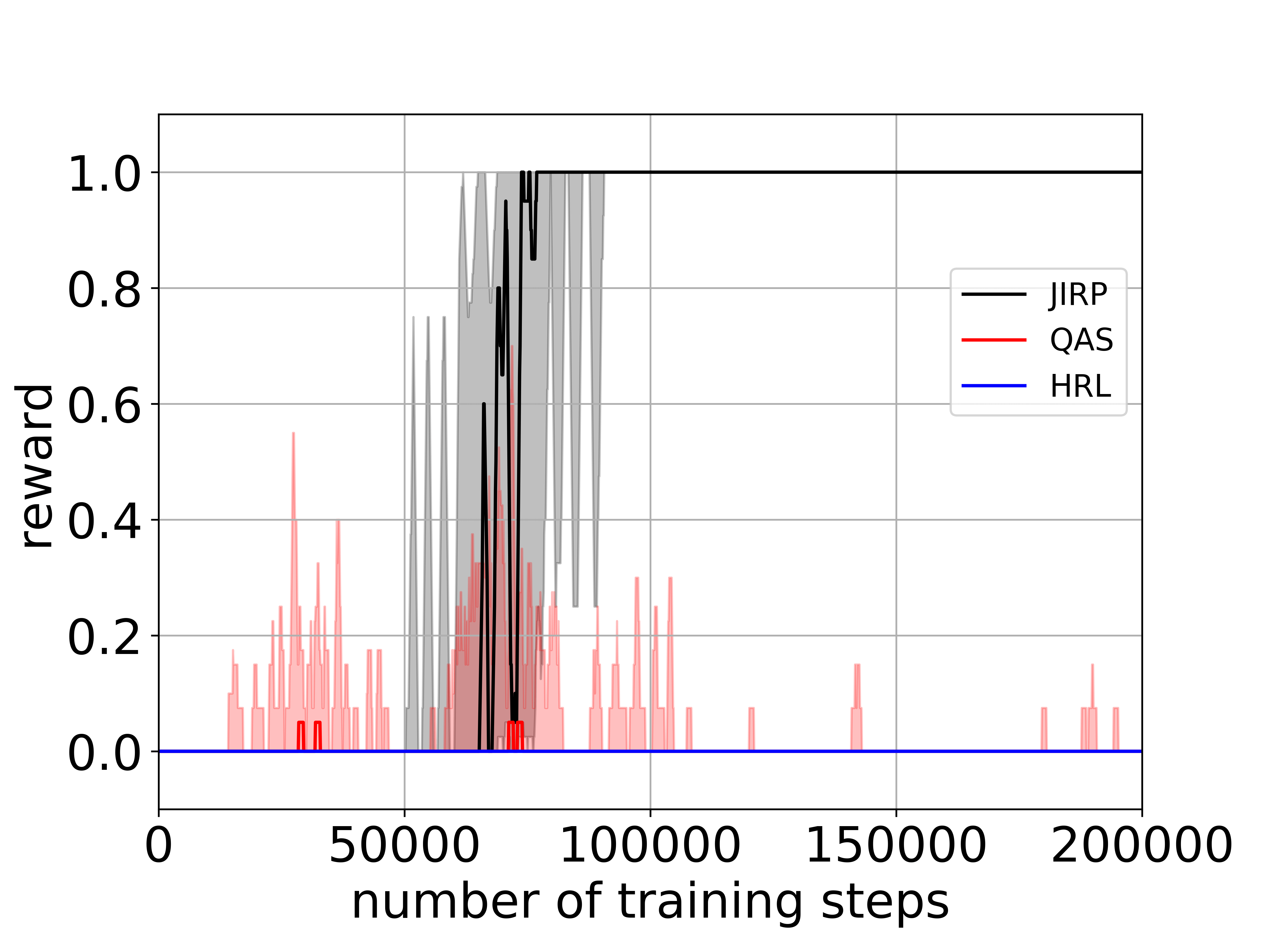
((a))

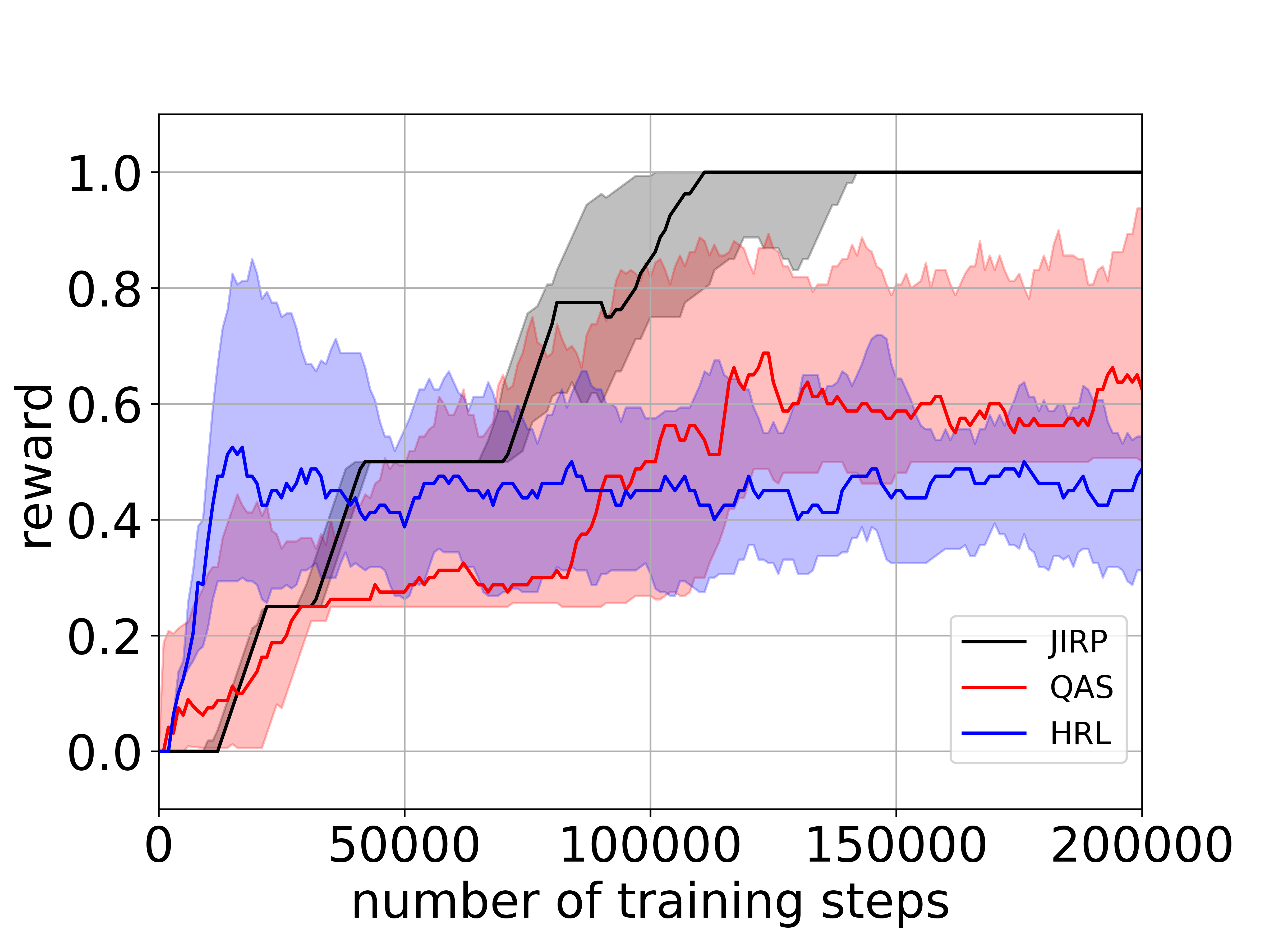
((b))

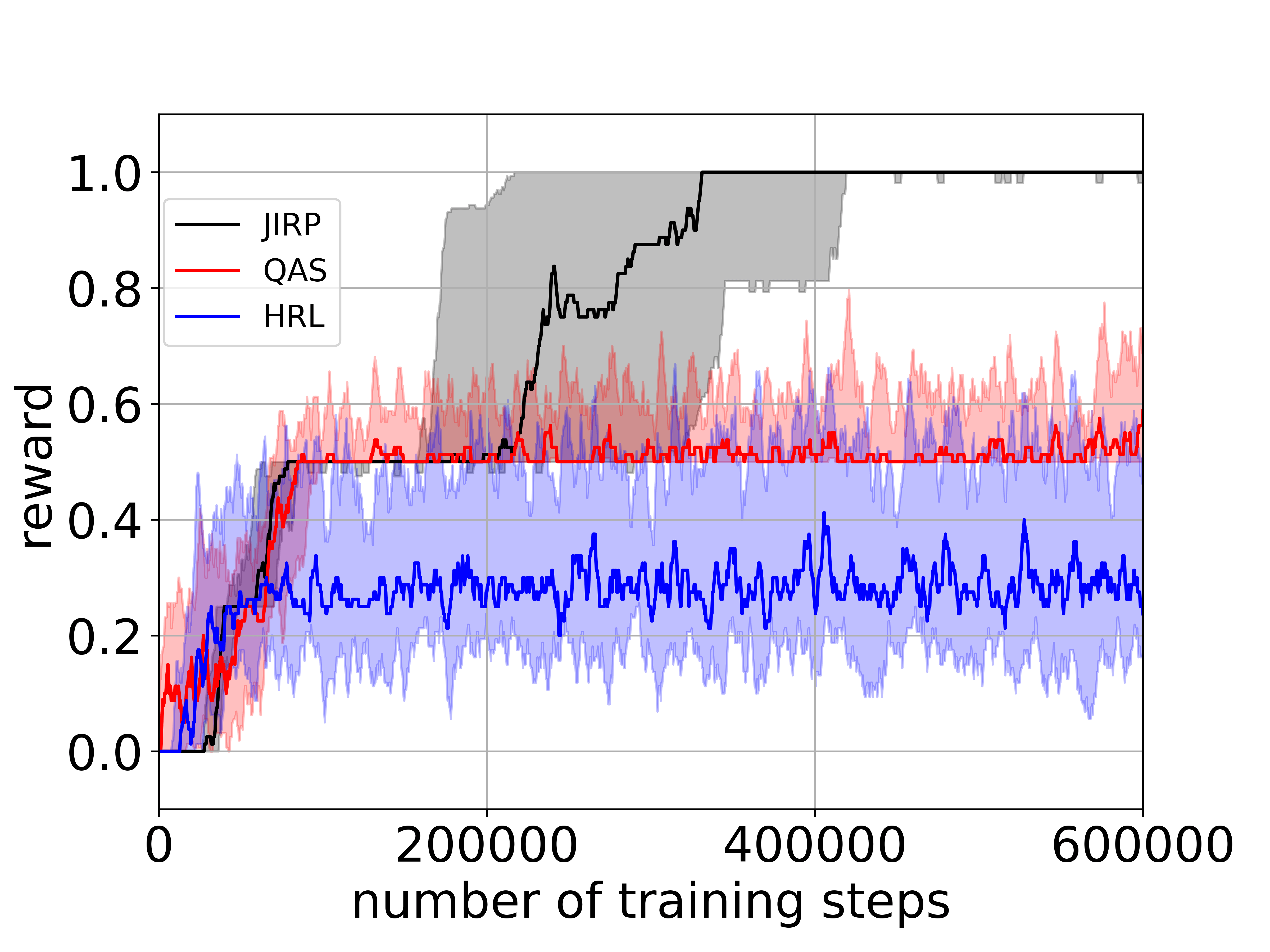
((c))

Figure 3: Cumulative rewards of 10 independent simulation runs averaged for every 10 training steps in (a) autonomous vehicle scenario; (b) office world scenario (averaged for four tasks); and (c) Minecraft world scenario (averaged for four tasks).

In this section, we apply the proposed approach to three different scenarios: 1) autonomous vehicle scenario; 2) office world scenario adapted from [13], and 3) Minecraft world scenario adapted from [10]. We use the libalf [27] implementation of RPNI [16] as the algorithm to infer reward machines. The detailed description of the tasks in the three different scenarios can be found in the supplementary material.

We compare JIRP (with algorithmic optimizations) with the two following baseline methods:

• QAS (q-learning in augmented state space): to incorporate the extra information of the labels (i.e., high-level events in the environment), we perform q-learning [14] in an augmented state space with an extra binary vector representing whether each label has been encountered or not.

• HRL (hierarchical reinforcement learning): we use a meta-controller for deciding the subtasks (represented by encountering each label) and use the low-level controllers expressed by neural networks [17] for deciding the actions at each state for each subtask.

5.1 Autonomous Vehicle Scenario

We consider the autonomous vehicle scenario as introduced in the motivating example in Section 1.1. The set of actions is $A=\{Straight,Left,Right,Stay\}$, corresponding to going straight, turning left, turning right and staying in place. For simplicity, we assume that the labeled MDP is deterministic (i.e, the slip rate is zero for each action). The vehicle will make a U-turn if it reaches the end of any road.

The set of labels is $\{\mathit{sp},\mathit{pr},\textrm{B}\}$ and the labeling function $L$ is defined by

$$\mathit{sp}\in L(s,a,s^{\prime}) \Leftrightarrow a=stay\wedge s\in\mathcal{J},$$

$$\mathit{pr}\in L(s,a,s^{\prime}) \Leftrightarrow s^{\prime}.priority=\top\wedge s\in\mathcal{J},$$

$$\textrm{B}\in L(s,a,s^{\prime}) \Leftrightarrow s^{\prime}.x=x_{\textrm{B}}\land s^{\prime}.y=y_{\textrm{B}},$$

where $s^{\prime}.priority$ is a Boolean variable that is true ($\top$) if and only if $s^{\prime}$ is on the priority roads, $\mathcal{J}$ represents the set of locations where the vehicle is entering an intersection, $s^{\prime}.x$ and $s^{\prime}.y$ are the $x$ and $y$ coordinate values at state $s$, and $x_{\textrm{B}}$ and $y_{\textrm{B}}$ are $x$ and $y$ coordinate values at B (see Figure 1).

We set $eplength=100$ and $N=100$. Figure 4 shows the inferred hypothesis reward machine in the last iteration of JIRP in one typical run. The inferred hypothesis reward machine is different from the true reward machine in Figure 2, but it can be shown that these two reward machines are equivalent on all attainable label sequences.

Figure 4: Inferred hypothesis reward machine in the last iteration of JIRP in one typical run in the autonomous vehicle scenario.

Figure 3 (a) shows the cumulative rewards with the three different methods in the autonomous vehicle scenario. The JIRP approach converges to optimal policies within 100,000 training steps, while QAS and HRL are stuck with near-zero cumulative reward for up to two million training steps (with the first 200,000 training steps shown in Figure 3 (a)).

5.2 Office World Scenario

We consider the office world scenario in the 9$\times$12 grid-world. The agent has four possible actions at each time step: move north, move south, move east and move west. After each action, the robot may slip to each of the two adjacent cells with probability of 0.05. We use four tasks with different high-level structural relationships among subtasks such as getting the coffee, getting mails and going to the office (see Appendix G for details).

We set $eplength=1000$ and $N=30$. Figure 3 (b) shows the cumulative rewards with the three different methods in the office world scenario. The JIRP approach converges to the optimal policy within 150,000 training steps, while QAS and HRL reach only 60% of the optimal average cumulative reward within 200,000 training steps.

5.3 Minecraft World Scenario

We consider the Minecraft example in a 21$\times$21 gridworld. The four actions and the slip rates are the same as in the office world scenario. We use four tasks including making plank, making stick, making bow and making bridge (see Appendix H for details).

We set $eplength=400$ and $N=30$. Figure 3 (c) shows the cumulative rewards with the three different methods in the Minecraft world scenario. The JIRP approach converges to the optimal policy within 400,000 training steps, while QAS and HRL reach only 50% of the optimal average cumulative reward within 600,000 training steps.

6 Conclusion

We proposed an iterative approach that alternates between reward machine inference and reinforcement learning (RL) for the inferred reward machine. We have shown the improvement of RL performances using the proposed method.

This work opens the door for utilizing automata learning in RL. First, the same methodology can be applied to other forms of RL, such as model-based RL, or actor-critic methods. Second, we will explore methods that can infer the reward machines incrementally (based on inferred reward machines in the previous iteration). Finally, the method to transfer the q-functions between equivalent states of reward machines can be also used for transfer learning between different tasks where the reward functions are encoded by reward machines.

Appendix A Proof of Lemma 1

Proof 1

We first prove that JIRP with $\mathit{eplength}\geq m$ explores every $m$-attainable trajectory with a positive (non-zero) probability. We show this claim by induction over the length $i$ of trajectories.

Base case:

The only trajectory of length $i=0$, $s_{I}$, is always explored because it is the initial state of every exploration.

Induction step:

Let $i=i^{\prime}+1$ and $\zeta=s_{0}a_{0}s_{1}\ldots s_{i^{\prime}}a_{i^{\prime}}s_{i}$ be an $m$-attainable trajectory of length $i\leq m$. Then, the induction hypothesis yields that JIRP explores each $m$-attainable trajectory $s_{0}a_{0}s_{1}\ldots s_{i^{\prime}}$ (of length $i^{\prime}=i-1$). Moreover JIRP continues its exploration because $\mathit{eplength}\geq m>i^{\prime}$. At this point, every action $a_{i^{\prime}}$ will be chosen with probability at least $\epsilon\times\frac{1}{|A_{s_{i^{\prime}}}|}$, where $A_{s_{i^{\prime}}}\subseteq A$ denotes the set of available actions in the state $s_{i^{\prime}}$ (this lower bound is due to the $\epsilon$-greedy strategy used in the exploration). Having chosen action $a_{i^{\prime}}$, the state $s_{i}$ is reached with probability $p(s_{i^{\prime}},a_{i^{\prime}},s_{i})>0$ because $\zeta$ is $m$-attainable. Thus, the trajectory $\zeta$ is explored with a positive probability.

Since JIRP with $\mathit{eplength}\geq m$ explores every $m$-attainable trajectory with a positive probability, the probability of an $m$-attainable trajectory not being explored becomes $0$ in the limit (i.e., when the number of episodes goes to infinity). Thus, JIRP almost surely (i.e., with probability $1$) explores every $m$-attainable trajectory in the limit.

Appendix B Proof of Lemma 2

In order to prove Lemma 2, we require a few (basic) definitions from automata and formal language theory.

An alphabet $\Sigma$ is a nonempty, finite set of symbols $b\in\Sigma$. A word $\omega=b_{0}\ldots b_{n}$ is a finite sequence of symbols. The empty sequence is called empty word and denoted by $\varepsilon$. The length of a word $\omega$, denoted by $|\omega|$ is the number of its symbols. We denote the set of all words over the alphabet $\Sigma$ by $\Sigma^{\ast}$.

Next, we recapitulate the definition of deterministic finite automata.

Definition 5

A deterministic finite automaton (DFA) is a five-tuple $\mathfrak{A}=(V,v_{I},\Sigma,\delta,F)$ consisting of a nonempty, finite set $V$ of states, an initial state $v_{I}\in V$, an input alphabet $\Sigma$, a transition function $\delta\colon V\times\Sigma\to V$, and a set $F\subseteq V$ of final states. The size of a DFA, denoted by $|\mathfrak{A}|$, is the number $|V|$ of its states.

A run of a DFA $\mathfrak{A}=(V,v_{I},\Sigma,\delta,F)$ on an input word $\omega=b_{0}\ldots b_{k}$ is a sequence $v_{0}\ldots v_{k+1}$ of states such that $v_{0}=v_{I}$ and $v_{i+1}=\delta(v_{i},b_{i})$ for each $i\in\{0,\ldots,k\}$. A run $v_{0}\ldots v_{k+1}$ of $\mathfrak{A}$ on a word $\omega$ is accepting if $v_{k+1}\in F$, and $\omega$ is accepted if there exists an accepting run. The language of a DFA $\mathfrak{A}$ is the set $L(\mathfrak{A})=\{\omega\in\Sigma^{\ast}\mid\text{$\mathfrak{A}$ accepts $\omega$}\}$. As usual, we call two DFAs $\mathfrak{A}_{1}$ and $\mathfrak{A}_{2}$ equivalent if $L(\mathfrak{A}_{1})=L(\mathfrak{A}_{2})$. Moreover, let us recapitulate the well-known fact that two non-equivalent DFAs have a “short” word that witnesses their non-equivalence.

Theorem 4 ([20], Theorem 3.10.5)

Let $\mathfrak{A}_{1}$ and $\mathfrak{A}_{2}$ be two DFAs with $L(\mathfrak{A}_{1})\neq L(\mathfrak{A}_{2})$. Then, there exists a word $\omega$ of length at most $|\mathfrak{A}_{1}|+|\mathfrak{A}_{2}|-1$ such that $\omega\in L(\mathfrak{A}_{1})$ if and only if $\omega\notin L(\mathfrak{A}_{2})$.

As the next step towards the proof of Lemma 2, we remark that every reward machine over the input alphabet $2^{\mathcal{P}}$ and output alphabet $\mathbb{R}$ can be translated into an “equivalent” DFA as defined below. This DFA operates over the combined alphabet $2^{\mathcal{P}}\times\mathbb{R}$ and accepts a word $(\ell_{0},r_{0})\ldots(\ell_{k},r_{k})$ if and only if $\mathcal{A}$ outputs the reward sequence $r_{0}\ldots r_{k}$ on reading the label sequence $\ell_{0}\ldots\ell_{k}$.

Lemma 3

Given a reward machine $\mathcal{A}=(V,{v_{I}},{2^{\mathcal{P}}},\mathbb{R},\delta,\sigma)$, one can construct a DFA $\mathfrak{A}_{\mathcal{A}}$ with $|\mathcal{A}|+1$ states such that

$$L(\mathfrak{A}_{\mathcal{A}})=\bigl{\{}(\ell_{0},r_{0})\ldots(\ell_{k},r_{k})\in(2^{\mathcal{P}}\times\mathbb{R})^{\ast}\mid\mathcal{A}(\ell_{0}\ldots\ell_{k})=r_{0}\ldots r_{k}\bigr{\}}.$$ (1)

Proof 2 (Proof of Lemma 3)

Let $\mathcal{A}=(V_{\mathcal{A}},v_{I,\mathcal{A}},2^{\mathcal{P}},\mathbb{R},\delta_{\mathcal{A}},\sigma_{\mathcal{A}})$ be a reward machine. Then, we define a DFA $\mathfrak{A}_{\mathcal{A}}=(V,v_{I},\Sigma,\delta,F)$ over the combined alphabet $2^{\mathcal{P}}\times\mathbb{R}$ by

• $V=V_{\mathcal{A}}\cup\{\bot\}$ with $\bot\notin V_{\mathcal{A}}$;

• $v_{I}=v_{I,\mathcal{A}}$;

• $\Sigma={2^{\mathcal{P}}}\times\mathbb{R}$;

• $\delta\bigl{(}v,(\ell,r)\bigr{)}=\begin{cases}v^{\prime}&\text{if $\delta_{\mathcal{A}}(v,\ell)=v^{\prime}$ and $\sigma_{\mathcal{A}}(v,\ell)=r$;}\\ \bot&\text{otherwise;}\end{cases}$

• $F=V_{\mathcal{A}}$.

In this definition, $\bot$ is a new sink state to which $\mathfrak{A}_{\mathcal{A}}$ moves if its input does not correspond to a valid input-output pair produced by $\mathcal{A}$. A straightforward induction over the length of inputs to $\mathfrak{A}_{\mathcal{A}}$ shows that it indeed accepts the desired language. In total, $\mathfrak{A}_{\mathcal{A}}$ has $|\mathcal{A}|+1$ states.

Similarly, one can construct a DFA $\mathfrak{A}_{\mathcal{M}}$ that accepts exactly the attainable traces of an MDP $\mathcal{M}$. First, viewing labels $L(s,a,s^{\prime})$ as input symbols, marking every state as an accepting state, and keeping only those transitions for which $p(s,a,s^{\prime})>0$, $\mathcal{M}$ can be viewed as a non-deterministic finite automaton. Second, using the standard determinization algorithm [20], one can create an equivalent DFA with an exponential blowup in the number of states.

Remark 1

Given a labeled MDP $\mathcal{M}$, one can construct a DFA $\mathfrak{A}_{\mathcal{M}}$ with at most $2^{|\mathcal{M}|}$ states that accepts exactly the admissible label sequences of $\mathcal{M}$.

Next, we show that if two reward machines disagree on an attainable label sequence, then we can provide a bound on the length of such a sequence.

Lemma 4

Let $\mathcal{M}=(S,s_{I},A,p,R,\gamma,\mathcal{P},L)$ be a labeled MDP and $\mathcal{A}_{1},\mathcal{A}_{2}$ two reward machines with input alphabet $2^{\mathcal{P}}$. If there exists an attainable label sequence $\lambda$ such that $\mathcal{A}_{1}(\lambda)\neq\mathcal{A}_{2}(\lambda)$, then there also exists an $m$-attainable label sequence $\lambda^{\star}$ with $m\leq 2^{|\mathcal{M}|}(|\mathcal{A}_{1}|+|\mathcal{A}_{2}|+2)-1$ such that $\mathcal{A}_{1}(\lambda^{\star})\neq\mathcal{A}_{2}(\lambda^{\star})$.

Proof 3 (Proof of Lemma 4)

Let $\mathcal{M}=(S,s_{I},A,p,R,\gamma,\mathcal{P},L)$ be a labeled MDP and $\mathcal{A}_{1}$, $\mathcal{A}_{2}$ two reward machines with input alphabet $2^{\mathcal{P}}$. As a first step, we construct the DFAs $\mathfrak{A}_{\mathcal{M}}=(V^{\prime},v^{\prime}_{I},2^{\mathcal{P}},\delta^{\prime},F^{\prime})$ according to Remark 1 and the DFAs $\mathfrak{A}_{\mathcal{A}_{i}}=(V^{\prime\prime}_{i},v^{\prime\prime}_{I,i},2^{\mathcal{P}}\times\mathbb{R},\delta^{\prime\prime}_{i},F^{\prime\prime}_{i})$ for $i\in\{1,2\}$ according to Lemma 3.

Next, we construct the input-synchronized product $\mathfrak{A}_{\mathcal{M}\times\mathcal{A}_{i}}=(V^{\prime\prime\prime},v^{\prime\prime\prime}_{I},2^{\mathcal{P}},\delta^{\prime\prime\prime},F^{\prime\prime\prime})$ of a $\mathfrak{A}_{\mathcal{M}}$ and $\mathfrak{A}_{\mathcal{A}_{i}}$ by

• $V^{\prime\prime\prime}=V^{\prime}\times V^{\prime\prime}_{i}$;

• $v^{\prime\prime\prime}_{I}=(v^{\prime}_{I},v^{\prime\prime}_{I,i})$;

• $\delta^{\prime\prime\prime}\bigl{(}(v^{\prime},v^{\prime\prime}_{i}),(\ell,r)\bigr{)}=\bigl{(}\delta^{\prime}(v^{\prime},\ell),\delta^{\prime\prime}_{i}(v^{\prime\prime}_{i},(\ell,r))\bigr{)}$; and

• $F^{\prime\prime\prime}=F^{\prime}\times F^{\prime\prime}_{i}$,

which synchronizes $\mathfrak{A}_{\mathcal{M}}$ and the input-component of $\mathfrak{A}_{\mathcal{A}_{i}}$. A straightforward induction over the lengths of inputs to $\mathfrak{A}_{\mathcal{M}\times\mathcal{A}_{i}}$ shows that $(\ell_{0},r_{0})\ldots(\ell_{k},r_{k})\in L(\mathfrak{A}_{\mathcal{M}\times\mathcal{A}_{i}})$ if and only if $\ell_{0}\ldots\ell_{k}$ is an attainable label sequence such that $\mathcal{A}_{i}(\ell_{0}\ldots\ell_{k})=r_{0}\ldots r_{k}$. Moreover, note that $\mathfrak{A}_{\mathcal{M}\times\mathcal{A}_{i}}$ has $2^{|\mathcal{M}|}(|\mathcal{A}_{i}|+1)$ states.

If there exists an attainable label sequence $\lambda$ such that $\mathcal{A}_{1}(\lambda)\neq\mathcal{A}_{2}(\lambda)$, then $L(\mathfrak{A}_{\mathcal{M}\times\mathcal{A}_{1}})\neq L(\mathfrak{A}_{\mathcal{M}\times\mathcal{A}_{2}})$ by construction of the DFAs $\mathfrak{A}_{\mathcal{M}\times\mathcal{A}_{1}}$ and $\mathfrak{A}_{\mathcal{M}\times\mathcal{A}_{2}}$. In this situation, Theorem 4 guarantees the existence of a word $\omega=(\ell_{0},r_{0})\ldots(\ell_{m-1},r_{m-1})\in(2^{\mathcal{P}}\times\mathbb{R})^{\ast}$ of size

$$m \leq 2^{|\mathcal{M}|}(|\mathcal{A}_{1}|+1)+2^{|\mathcal{M}|}(|\mathcal{A}_{2}|+1)-1$$

$$=2^{|\mathcal{M}|}(|\mathcal{A}_{1}|+|\mathcal{A}_{2}|+2)-1$$

such that $\omega\in L(\mathfrak{A}_{\mathcal{M}\times\mathcal{A}_{1}})$ if and only if $\omega\notin L(\mathfrak{A}_{\mathcal{M}\times\mathcal{A}_{2}})$.

Let now $\lambda^{\star}=\ell_{0}\ldots\ell_{m-1}$. By construction of the DFAs $\mathfrak{A}_{\mathcal{M}\times\mathcal{A}_{1}}$ and $\mathfrak{A}_{\mathcal{M}\times\mathcal{A}_{2}}$, we know that $\mathcal{A}_{1}(\lambda^{\star})\neq\mathcal{A}_{2}(\lambda^{\star})$ holds. Moreover, $\lambda^{\star}$ is an $m$-attainable label sequence with the desired bound on $m$.

We are now ready to prove Lemma 2.

Proof 4 (Proof of Lemma 2)

Let $X_{0},X_{1},\ldots$ be the sequence of samples that arise in the run of JIRP whenever new counterexamples are added to $X$ (in Line 2 of Algorithm 2). We now make two observations about this sequence, which help us prove Lemma 2.

1. The sequence $X_{0},X_{1},\ldots$ grows strictly monotonically (i.e., $X_{0}\subsetneq X_{1}\subsetneq\cdots$). The reasons for this are twofold. First, JIRP always adds counterexamples to $X$ and never removes them (which establishes $X_{0}\subseteq X_{1}\subseteq\cdots$). Second, whenever a counterexample $(\lambda_{i},\rho_{i})$ is added to $X_{i}$ to form $X_{i+1}$, then $(\lambda_{i},\rho_{i})\notin X_{i}$. To see why this is the case, remember that JIRP always constructs hypothesis reward machines that are consistent with the current sample. Thus, the reward machine $\mathcal{H}_{i}$ is consistent with $X_{i}$. However, $(\lambda_{i},\rho_{i})$ was added because $\mathcal{H}_{i}(\lambda_{i})\neq\rho_{i}$. Hence, $(\lambda_{i},\rho_{i})$ cannot have been an element of $X_{i}$.

2. The true reward machine $\mathcal{A}$, the one that encodes the reward function $R$, is by definition consistent with all samples $X_{i}$ that are generated during the run of JIRP.

Once a new counterexample is added, JIRP learns a new reward machine. Let $\mathcal{H}_{0},\mathcal{H}_{1},\ldots$ be the sequence of these reward machines, where $\mathcal{H}_{i}$ is computed based on the sample $X_{i}$. As above, we make two observations about this sequence.

1. We have $|\mathcal{H}_{i}|\leq|\mathcal{H}_{i+1}|$. Towards a contradiction, assume that $|\mathcal{H}_{i}|>|\mathcal{H}_{i+1}|$. Since JIRP always computes consistent reward machines and $X_{i}\subsetneq X_{i+1}$ (see Observation 1), we know that $\mathcal{H}_{i+1}$ is not only consistent with $X_{i+1}$ but also with $X_{i}$ (by definition of consistency). Moreover, JIRP always computes consistent reward machines of minimal size. Thus, since $\mathcal{H}_{i+1}$ is consistent with $X_{i}$ and $|\mathcal{H}_{i+1}|<|\mathcal{H}_{i}|$, the reward machine $\mathcal{H}_{i}$ is not minimal, which yields the desired contradiction.

2. We have $\mathcal{H}_{i}\neq\mathcal{H}_{j}$ for each $j\in\{0,\ldots,i-1\}$; in other words, the reward machines generated during the run of JIRP are semantically distinct. This is a consequence of the facts that $(\lambda_{j},\rho_{j})$ was a counterexample to $\mathcal{H}_{j}$ (i.e., $\mathcal{H}_{j}(\lambda_{j})\neq\rho_{j}$) and the learning algorithm for reward machines always constructs consistent reward machines (which implies $\mathcal{H}_{i}(\lambda_{j})=\rho_{j}$).

Observations 2 and 3 now provide $|\mathcal{A}|$ as an upper bound on the size of the hypothesis reward machines constructed in the run of JIRP. Since there are only finite many reward machines of size $|\mathcal{A}|$ or less, Observation 4 then implies that there exists an $i^{\star}\in\mathbb{N}$ after which no new reward machine is inferred. Thus, it is left to show that $\mathcal{H}_{i^{\star}}(\lambda)=\mathcal{A}(\lambda)$ for all attainable label sequences $\lambda$.

Towards a contradiction, assume that there exists an attainable label sequence $\lambda$ such that $\mathcal{H}_{i^{\star}}(\lambda)\neq\mathcal{A}(\lambda)$. Lemma 4 then guarantees the existence of an $m$-attainable label sequence $\lambda^{\star}$ with

$$m \leq 2^{|\mathcal{M}|}(|\mathcal{H}_{i^{\star}}|+|\mathcal{A}|+2)-1$$

$$\leq 2^{|\mathcal{M}|}(2|\mathcal{A}|+2)-1$$

$$=2^{|\mathcal{M}|+1}(|\mathcal{A}|+1)-1$$

such that $\mathcal{H}_{i^{\star}}(\lambda^{\star})\neq\mathcal{A}(\lambda^{\star})$. By Corollary 1, JIRP almost surely explores the label sequence $\lambda^{\star}$ in the limit because we assume $\mathit{eplength}\geq 2^{|\mathcal{M}|+1}(|\mathcal{A}|+1)-1=m$. Thus, the trace $(\lambda^{\star},\rho^{\star})$, where $\rho^{\star}=\mathcal{A}(\lambda^{\star})$, is almost surely returned as a new counterexample, resulting in a new sample $X_{i^{\star}+1}$. This triggers the construction of a new reward machine $\mathcal{H}_{i^{\star}+1}$ (which will then be different from all previous reward machines). However, this contradicts the assumption that no new reward machine is constructed after $\mathcal{H}_{i^{\star}}$. Thus, $\mathcal{H}_{i^{\star}}(\lambda)=\mathcal{A}(\lambda)$ holds for all attainable input sequences $\lambda$.

Appendix C Proof of Theorem 1

To prove Theorem 1, we use the fact that JIRP will eventually learn a reward machine equivalent to the reward machine $\mathcal{A}$ on all attainable label sequences (see Lemma 2). Then, closely following the proof of Theorem 4.1 from [13], we construct an MDP $\mathcal{M}_{\mathcal{A}}$, show that using the same policy for $\mathcal{M}$ and $\mathcal{M}_{\mathcal{A}}$ yields same rewards, and, due to convergence of q-learning for $\mathcal{M}_{\mathcal{A}}$, conlcude that JIRP converges towards an optimal policy for $\mathcal{M}$. Lemma 5 describes the construction of the mentioned MDP $\mathcal{M}_{\mathcal{A}}$.

Lemma 5

Given an MDP $\mathcal{M}=(S,s_{I},A,p,R,\gamma,\mathcal{P},L)$ with a non-Markovian reward function defined by a reward machine $\mathcal{A}=(V,v_{I},2^{\mathcal{P}},\mathbb{R},\delta,\sigma)$, one can construct an MDP $\mathcal{M}_{\mathcal{A}}$ whose reward function is Markovian such that every attainable label sequence of $\mathcal{M}_{\mathcal{A}}$ gets the same reward as in $\mathcal{M}$. Furthermore, any policy for $\mathcal{M}_{\mathcal{A}}$ achieves the same expected reward in $\mathcal{M}$.

Proof 5

Let $\mathcal{M}=(S,s_{I},A,p,R,\gamma,\mathcal{P},L)$ be a labeled MDP and $\mathcal{A}=(V,{v_{I}},2^{\mathcal{P}},\mathbb{R},\delta,\sigma)$ a reward machine encoding its reward function. We define the product MDP $\mathcal{M}_{\mathcal{A}}=(S^{\prime},s^{\prime}_{I},A,p^{\prime},R^{\prime},\gamma^{\prime},\mathcal{P}^{\prime},L^{\prime})$ by

• $S^{\prime}=S\times V$;

• $s^{\prime}_{I}=(s_{I},v_{I})$;

• $A=A$;

• $p^{\prime}\bigl{(}(s,v),a,(s^{\prime},v^{\prime})\bigr{)}$
  $=\begin{cases}p(s,a,s^{\prime})&v^{\prime}=\delta(v,L(s,a,s^{\prime}));\\ 0&\text{otherwise};\end{cases}$

• $\mathcal{P}^{\prime}=\mathcal{P}$; $L^{\prime}=L$;

• $R^{\prime}\bigl{(}(s,v),a,(s^{\prime},v^{\prime})\bigr{)}=\sigma\bigl{(}v,L(s,a,s^{\prime})\bigr{)}$; and

• $\gamma^{\prime}=\gamma$.

The described MDP has a Markovian reward function that matches $R$, the (non-Markovian) reward function of $\mathcal{M}$ defined by the reward machine $\mathcal{A}$ (Definition 2). Since the reward functions and discount factors are the same, the claims follow.

Lemma 2 shows that eventually $\mathcal{H}$, the reward machine learned by JIRP, will be equivalent to $\mathcal{A}$ on all attainable label sequences. Thus, using Lemma 5, an optimal policy for MDP $\mathcal{M}_{\mathcal{H}}$ will also be optimal for $\mathcal{M}$.

When running episodes of QRM (Algorithm 1) under the reward machine $\mathcal{H}$, an update of a $q$-function connected to a state of a reward machine corresponds to updating the $q$ function for $\mathcal{M}_{\mathcal{H}}$. Because $\textit{eplength}\geq|\mathcal{M}|$, the fact that QRM uses $\epsilon$-greedy strategy and that updates are done in parallel for all states of the reward machine $\mathcal{H}$, we know that every state-action pair of the MDP $\mathcal{M}_{\mathcal{H}}$ will be seen infinitely often. Hence, convergence of q-learning for $\mathcal{M}_{\mathcal{H}}$ to an optimal policy is guaranteed [14]. Finally, because of Lemma 5, JIRP converges to an optimal policy, too.

We have proved that if the number of episodes goes to infinity, and the length of an episode is at least $2^{|\mathcal{M}|+1}(|\mathcal{A}|+1)-1$, then JIRP converges towards an optimal policy.

Appendix D Proof of Theorem 2

In order to prove Theorem 2, we first need to prove the following lemma.

Lemma 6

Let $\mathcal{M}$ be a labeled MDP and $\mathcal{A}$ the reward machine encoding the rewards of $\mathcal{M}$. Then, JIRP with Optimizations 1 and 2 with $\mathit{eplength}\geq 2^{|\mathcal{M}|+1}(|\mathcal{A}|+1)-1$ learns a reward machine that is equivalent to $\mathcal{A}$ on all attainable traces in the limit (i.e., when the number of episodes goes to infinity).

Proof 6

With Optimizations 1 and 2, let $X_{0},X_{1},\ldots$ (with slight abuse of notation from the proof of Lemma 2) be the sequence of sets that arise in the run of JIRP with the algorithmic optimizations whenever the non-empty set of new counterexamples $X_{\textrm{new}}$ are added to the set $X$. Then, it can be shown that Observation 1, 2, 3 and 4 in the proof of Lemma 2 still hold and thus Lemma 6 holds.

With Lemma 6 and following the analysis in the proofs of Theorem 1, Theorem 2 holds.

Appendix E Proof of Theorem 3

To prove Theorem 3, we first recapitulate the definition of $k$-horizon optimal discounted action value functions [28].

Definition 6

Let $\mathcal{A}=(V,{v_{I}},2^{\mathcal{P}},\mathbb{R},\delta,\sigma)$ be a reward machine encoding the rewards of a labeled MDP $\mathcal{M}=(S,s_{I},A,p,R,\gamma,\mathcal{P},L)$. We define the $k$-horizon optimal discounted action value function $q^{\ast v}_{k}(s,a)$ recursively as follows:

$$\begin{split}q^{\ast v}_{k}(s,a)=&\sum_{v^{\prime}\in V}\sum_{s^{\prime}\in S}T(s,v,a,s^{\prime},v^{\prime})\\ &\times[\sigma(v,L(s,a,s^{\prime}))+\gamma\max_{a^{\prime}\in A}q^{\ast v^{\prime}}_{k-1}(s^{\prime},a^{\prime})],\end{split}$$

where

$$T(s,v,a,s^{\prime},v^{\prime})=\begin{cases}p(s,a,s^{\prime}),~{}~{}\mbox{if}~{}v^{\prime}=\delta(v,L(s,a,s^{\prime}));\\ 0,~{}~{}~{}~{}~{}~{}~{}~{}~{}~{}~{}~{}~{}~{}~{}~{}~{}\mbox{otherwise},\end{cases}$$

and $q^{\ast v}_{0}(s,a)=0$ for every $v\in V$, $s\in S$ and $a\in A$.

We then give the following lemma based on the equivalent relationship formalized in Definition 4.

Lemma 7

Let $\mathcal{A}=(V,{v_{I}},2^{\mathcal{P}},\mathbb{R},\delta,\sigma)$ and $\hat{\mathcal{A}}=(\hat{V},{\hat{v}_{I}},2^{\mathcal{P}},\mathbb{R},\hat{\delta},\hat{\sigma})$ be two reward machines encoding the rewards of a labeled MDP $\mathcal{M}=(S,s_{I},A,p,R,\gamma,\mathcal{P},L)$. For state $v\in V$ and state $\hat{v}\in\hat{V}$, if $v\sim\hat{v}$, then for every $u\in{2^{\mathcal{P}}}$, we have $\delta(v,u)\sim\hat{\delta}(\hat{v},u)$.

Proof 7

For a Mealy machine $\mathcal{A}=(V,{v_{I}},{2^{\mathcal{P}}},\mathbb{R},\delta,\sigma)$, we extend the output function $\sigma$ to an output function $\sigma^{+}\colon V\times({2^{\mathcal{P}}})^{+}\to\sigma^{+}$ over (nonempty) words: $\sigma^{+}(v,u)=\sigma(v,u)$ and $\sigma^{+}(v,u\cdot\lambda)=\sigma(v,u)\cdot\sigma^{+}(\delta(v,u),\lambda)$, for every $v\in V$, $u\in{2^{\mathcal{P}}}$, and $\lambda\in({2^{\mathcal{P}}})^{+}$, where we use $\cdot$ to denote concatenation.

For two Mealy machines $\mathcal{A}=(V,{v_{I}},{2^{\mathcal{P}}},\mathbb{R},\delta,\sigma)$, and $\hat{\mathcal{A}}=(\hat{V},{\hat{v}_{I}},{2^{\mathcal{P}}},\mathbb{R},\hat{\delta},\hat{\sigma})$ (over the same input and output alphabet), two states $v\in V,\hat{v}\in\hat{V}$ and any label sequence $\lambda$, we have $\mathcal{A}[v](\lambda)=\hat{\mathcal{A}}[\hat{v}](\lambda)$, if and only if $\sigma^{+}(v,\lambda)=\hat{\sigma}^{+}(\hat{v},\lambda)$. Therefore, from Definition 4 we have $v\sim\hat{v}$ if and only if $\sigma^{+}(v,\lambda)=\hat{\sigma}^{+}(\hat{v},\lambda)$ for all $\lambda\in({2^{\mathcal{P}}})^{+}$.

Thus, we have

$$\sigma^{+}(\delta(v,u),\lambda) =\sigma^{+}(v,u\cdot\lambda)$$

$$\stackrel{{\scriptstyle\text{(a)}}}{{=}}\hat{\sigma}^{+}(\hat{v},u\cdot\lambda)$$ (2)

$$=\hat{\sigma}^{+}(\hat{\delta}(\hat{v},u),\lambda),$$

where (a) follows from the equivalence of $v$ and $\hat{v}$. Therefore, for every $u\in{2^{\mathcal{P}}}$, we have $\mathcal{A}[\delta(v,u)](\lambda)=\hat{\mathcal{A}}[\hat{\delta}(\hat{v},u)](\lambda)$ holds for all label sequences $\lambda$.

With Definition 6 and Lemma 7, we proceed to prove that for two equivalent states, the corresponding $k$-horizon optimal discounted action value functions are the same (as formalized in the following lemma).

Lemma 8

Let $\mathcal{A}=(V,{v_{I}},2^{\mathcal{P}},\mathbb{R},\delta,\sigma)$ and $\hat{\mathcal{A}}=(\hat{V},{\hat{v}_{I}},2^{\mathcal{P}},\mathbb{R},\hat{\delta},\hat{\sigma})$ be two reward machines encoding the rewards of a labeled MDP $\mathcal{M}=(S,s_{I},A,p,R,\gamma,\mathcal{P},L)$. For states $v\in V$ and $\hat{v}\in\hat{V}$, if $v\sim\hat{v}$, then for every $s\in S$ and $a\in A$, $q^{\ast v}_{k}(s,a)=q^{\ast\hat{v}}_{k}(s,a)$ for every $k$.

Proof 8

We use induction to prove Lemma 8. For $k=1$, we have for every $s\in S$ and $a\in A$,

$$\begin{split}q^{\ast v}_{1}(s,a)&=\sum_{v^{\prime}\in V}\sum_{s^{\prime}\in S}T(s,v,a,s^{\prime},v^{\prime})\sigma(v,L(s,a,s^{\prime}))\\ &=\sum_{s^{\prime}\in S}T(s,v,a,s^{\prime},\delta(v,L(s,a,s^{\prime})))\sigma(v,L(s,a,s^{\prime}))\\ &=\sum_{s^{\prime}\in S}p(s,a,s^{\prime})\sigma(v,L(s,a,s^{\prime}))\\ &\stackrel{{\scriptstyle\text{(b)}}}{{=}}\sum_{s^{\prime}\in S}p(s,a,s^{\prime})\hat{\sigma}(\hat{v},L(s,a,s^{\prime}))\\ &=\sum_{s^{\prime}\in S}\hat{T}(s,\hat{v},a,s^{\prime},\hat{\delta}(\hat{v},L(s,a,s^{\prime})))\hat{\sigma}(\hat{v},L(s,a,s^{\prime}))\\ &=\sum_{\hat{v}^{\prime}\in\hat{V}}\sum_{s^{\prime}\in S}\hat{T}(s,\hat{v},a,s^{\prime},\hat{v}^{\prime})\hat{\sigma}(\hat{v},L(s,a,s^{\prime}))\\ &=q^{\ast\hat{v}}_{1}(s,a)\end{split}$$

where the equality (b) comes from the fact that $v\sim\hat{v}$, and

$$\hat{T}(s,\hat{v},a,s^{\prime},\hat{v}^{\prime})=\begin{cases}p(s,a,s^{\prime}),~{}~{}\mbox{if}~{}\hat{v}^{\prime}=\hat{\delta}(\hat{v},L(s,a,s^{\prime}));\\ 0,~{}~{}~{}~{}~{}~{}~{}~{}~{}~{}~{}~{}~{}~{}~{}~{}~{}\mbox{otherwise}.\end{cases}$$

Now we assume that for every state $v\in V$ and state $\hat{v}\in\hat{V}$, if $v\sim\hat{v}$, then we have that $q^{\ast v}_{k-1}(s,a)=q^{\ast\hat{v}}_{k-1}(s,a)$ holds for every $s\in S$ and every $a\in A$. We proceed to prove that for every state $v\in V$ and state $\hat{v}\in\hat{V}$, if $v\sim\hat{v}$, then we have that $q^{\ast v}_{k}(s,a)=q^{\ast\hat{v}}_{k}(s,a)$ holds for every $s\in S$ and every $a\in A$.

For every $s\in S$ and every $a\in A$, we have

$$\begin{split}q^{\ast v}_{k}(s,a)&=\sum_{v^{\prime}\in V}\sum_{s^{\prime}\in S}T(s,v,a,s^{\prime},v^{\prime})\\ &\times[\sigma(v,L(s,a,s^{\prime}))+\gamma\max_{a^{\prime}\in A}q^{\ast v^{\prime}}_{k-1}(s^{\prime},a^{\prime})]\\ &=\sum_{s^{\prime}\in S}T(s,v,a,s^{\prime},\delta(v,L(s,a,s^{\prime})))\\ &\times[\sigma(v,L(s,a,s^{\prime}))+\gamma\max_{a^{\prime}\in A}q^{\ast\delta(v,L(s,a,s^{\prime}))}_{k-1}(s^{\prime},a^{\prime})]\\ &=\sum_{s^{\prime}\in S}p(s,a,s^{\prime})\\ &\times[\sigma(v,L(s,a,s^{\prime}))+\gamma\max_{a^{\prime}\in A}q^{\ast\delta(v,L(s,a,s^{\prime}))}_{k-1}(s^{\prime},a^{\prime})]\\ &\stackrel{{\scriptstyle\text{(c)}}}{{=}}\sum_{s^{\prime}\in S}p(s,a,s^{\prime})\\ &\times[\hat{\sigma}(\hat{v},L(s,a,s^{\prime}))+\gamma\max_{a^{\prime}\in A}q^{\ast\hat{\delta}(\hat{v},L(s,a,s^{\prime}))}_{k-1}(s^{\prime},a^{\prime})]\\ &=\sum_{s^{\prime}\in S}\hat{T}(s,\hat{v},a,s^{\prime},\hat{\delta}(\hat{v},L(s,a,s^{\prime})))\\ &\times[\sigma(\hat{v},L(s,a,s^{\prime}))+\gamma\max_{a^{\prime}\in A}q^{\ast\hat{\delta}(\hat{v},L(s,a,s^{\prime}))}_{k-1}(s^{\prime},a^{\prime})]\\ &=\sum_{\hat{v}^{\prime}\in\hat{V}}\sum_{s^{\prime}\in S}\hat{T}(s,\hat{v},a,s^{\prime},\hat{v}^{\prime})\\ &\times[\sigma(\hat{v},L(s,a,s^{\prime}))+\gamma\max_{a^{\prime}\in A}q^{\ast\hat{\delta}(\hat{v},L(s,a,s^{\prime}))}_{k-1}(s^{\prime},a^{\prime})]\end{split}$$ (3)

$$=q^{\ast\hat{v}}_{k}(s,a)$$

where the equality (c) comes from the fact that $v\sim\hat{v}$ and $\delta(v,L(s,a,s^{\prime}))\sim\hat{\delta}(\hat{v},L(s,a,s^{\prime}))$ (according to Lemma 7).

Therefore, it is proven by induction that Lemma 8 holds.

With Lemma 8, we now proceed to prove Theorem 3. According to Lemma 8, if $v\sim\hat{v}$, then for every $s\in S$ and $a\in A$, $q^{\ast v}_{k}(s,a)=q^{\ast\hat{v}}_{k}(s,a)$ for every $k$. When $k\rightarrow\infty$, $q^{\ast}_{k}(v,s,a)$ and $q^{\ast}_{k}(\hat{v},s,a)$ converge to the fixed points as follows.

$$\begin{split}q^{\ast v}(s,a)=&\sum_{v^{\prime}\in V}\sum_{s^{\prime}\in S}T(s,v,a,s^{\prime},v^{\prime})\\ &\times[\sigma(v,L(s,a,s^{\prime}))+\gamma\max_{a^{\prime}\in A}q^{\ast v^{\prime}}(s^{\prime},a^{\prime})],\\ q^{\ast\hat{v}}(s,a)=&\sum_{\hat{v}^{\prime}\in\hat{V}}\sum_{s^{\prime}\in S}T(s,\hat{v},a,s^{\prime},\hat{v}^{\prime})\\ &\times[\hat{\sigma}(\hat{v},L(s,a,s^{\prime}))+\gamma\max_{a^{\prime}\in A}q^{\ast\hat{v}^{\prime}}(s^{\prime},a^{\prime})].\end{split}$$

Therefore, for every $s\in S$ and $a\in A$, $q^{\ast v}(s,a)=q^{\ast\hat{v}}(s,a)$.

Appendix F Details in Autonomous Vehicle Scenario

We provide the detailed results in autonomous vehicle scenario. Figure 5 shows the gridded map of the roads in a residential area. The set of actions is $A=\{Straight,Left,Right,Stay\}$, corresponding to going straight, turning left, turning right and staying in place. We use a simplified version of transitions at the intersections. For example, at (1,7), if the vehicle stays, then it ends at (1, 7); if the vehicle goes straight, then it ends at (4, 7) at the next step; if the vehicle turns left, then it ends at (3, 9) at the next step; and if the vehicle turns right, then it ends at (2, 6) at the next step. The vehicle will make a U-turn if it reaches the end of any road. For example, if the vehicle reaches (10, 7), then it will reach (10, 8) at the next step.

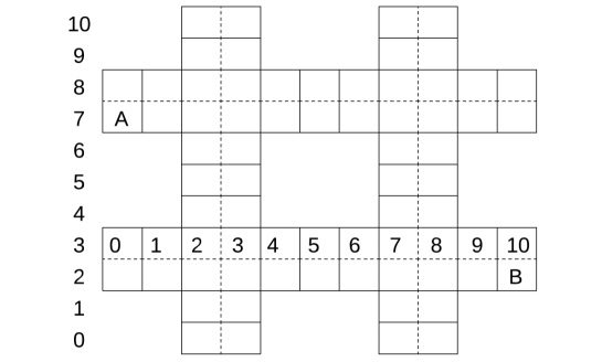
Figure 5: Gridded map of a residential area in autonomous vehicle scenario.

Figure 6 shows the cumulative rewards of 10 independent simulation runs averaged for every 10 training steps for the autonomous vehicle scenario.

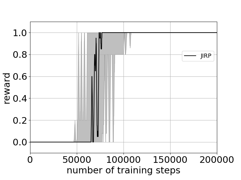
((a))

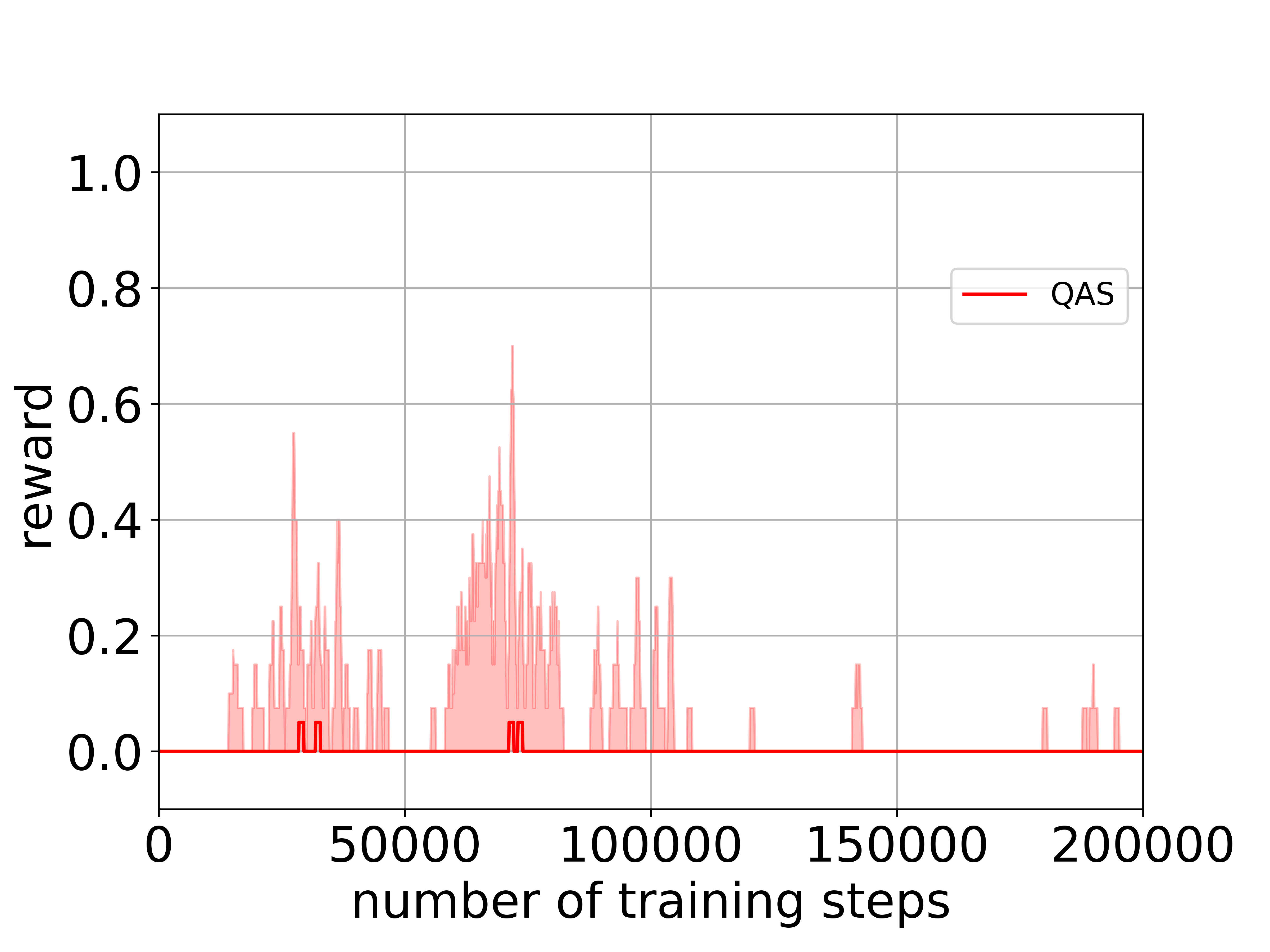
((b))

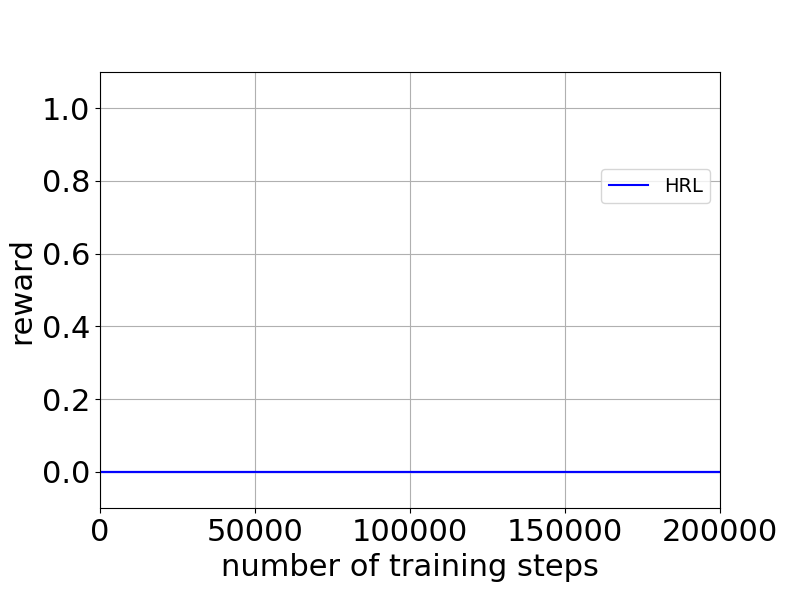
((c))

Figure 6: Cumulative rewards of 10 independent simulation runs averaged for every 10 training steps in the autonomous vehicle scenario: (a) JIRP; (b) QAS; (c) HRL.

Appendix G Details in Office World Scenario

We provide the detailed results in the office world scenario. Figure 7 shows the map in the office world scenario. We use the triangle to denote the initial position of the agent. We consider the following four tasks:
Task 2.1: get coffee at c and deliver the coffee to the office o;
Task 2.2: get mail at m and deliver the coffee to the office o;
Task 2.3: go to the office o, then get coffee at c and go back to the office o, finally go to mail at m;
Task 2.4: get coffee at c and deliver the coffee to the office o, then come to get coffee at c and deliver the coffee to the frontdesk d.

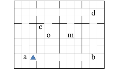
Figure 7: The map in the office world scenario.

G.1 Task 2.1

For task 2.1, Figure 8 shows the inferred hypothesis reward machine in the last iteration of JIRP. Figure 9 shows the cumulative rewards of 10 independent simulation runs averaged for every 10 training steps for task 2.1.

Figure 8: The inferred hypothesis reward machine for task 2.1  in the last iteration of JIRP.

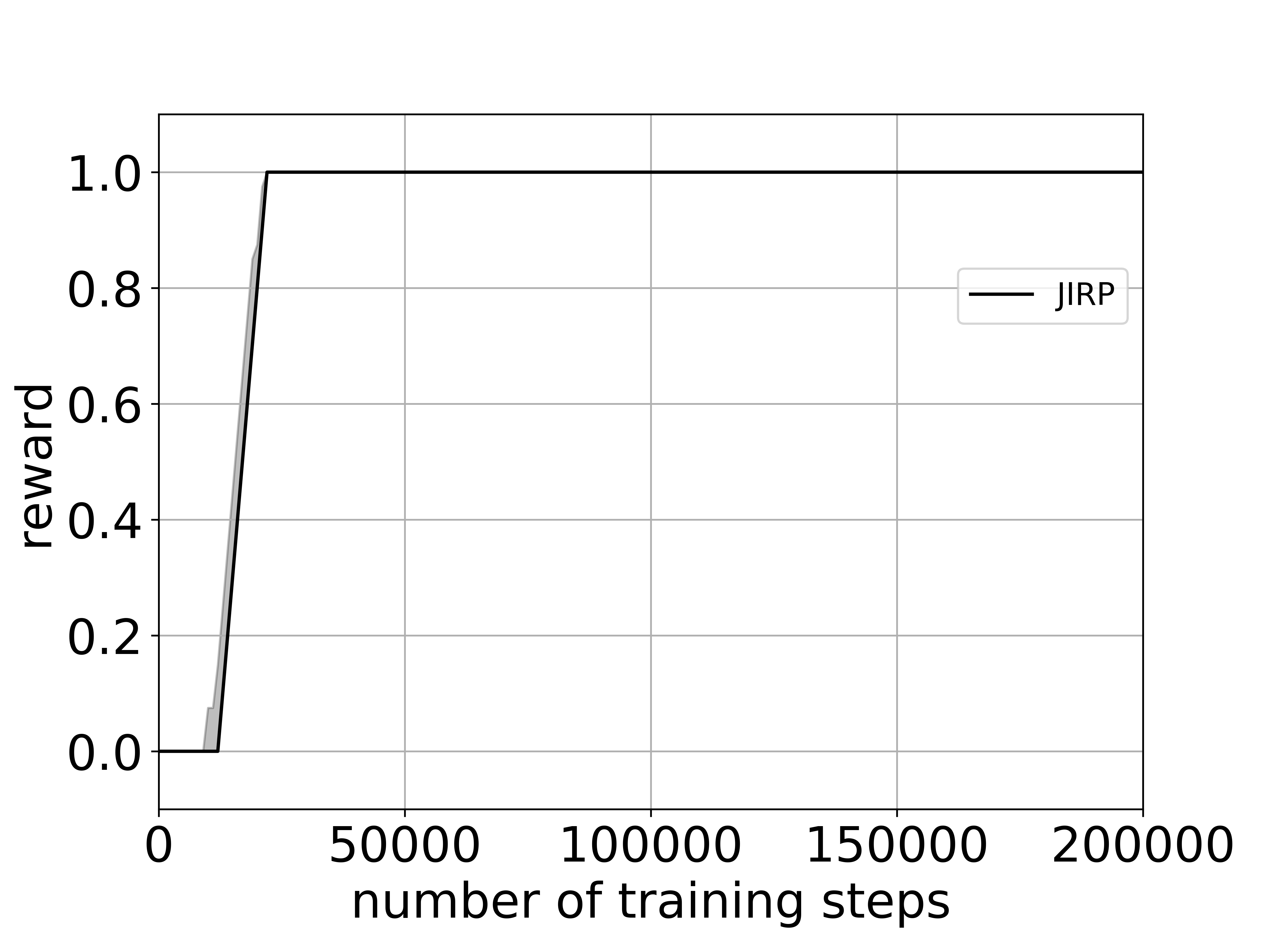
((a))

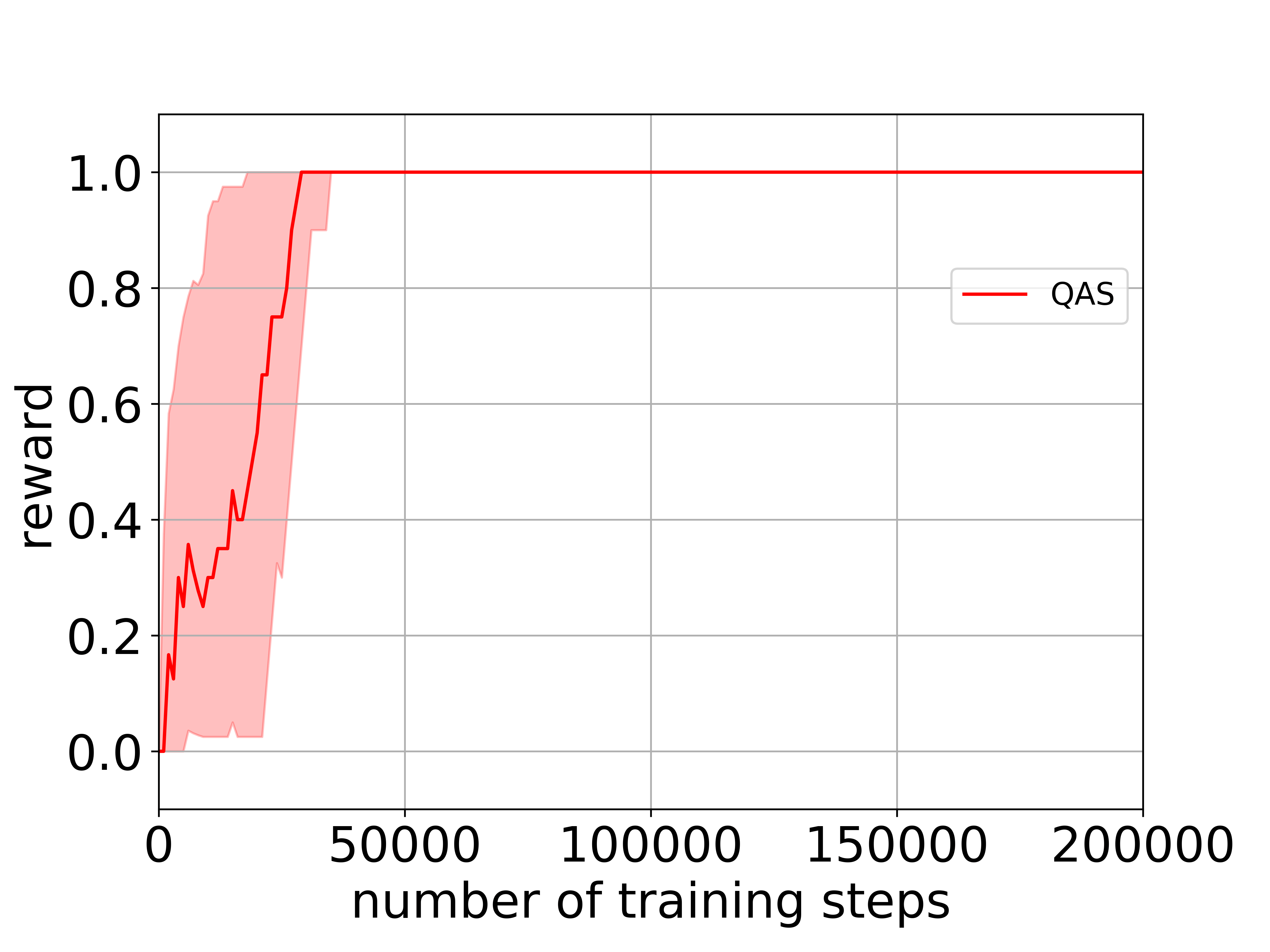
((b))

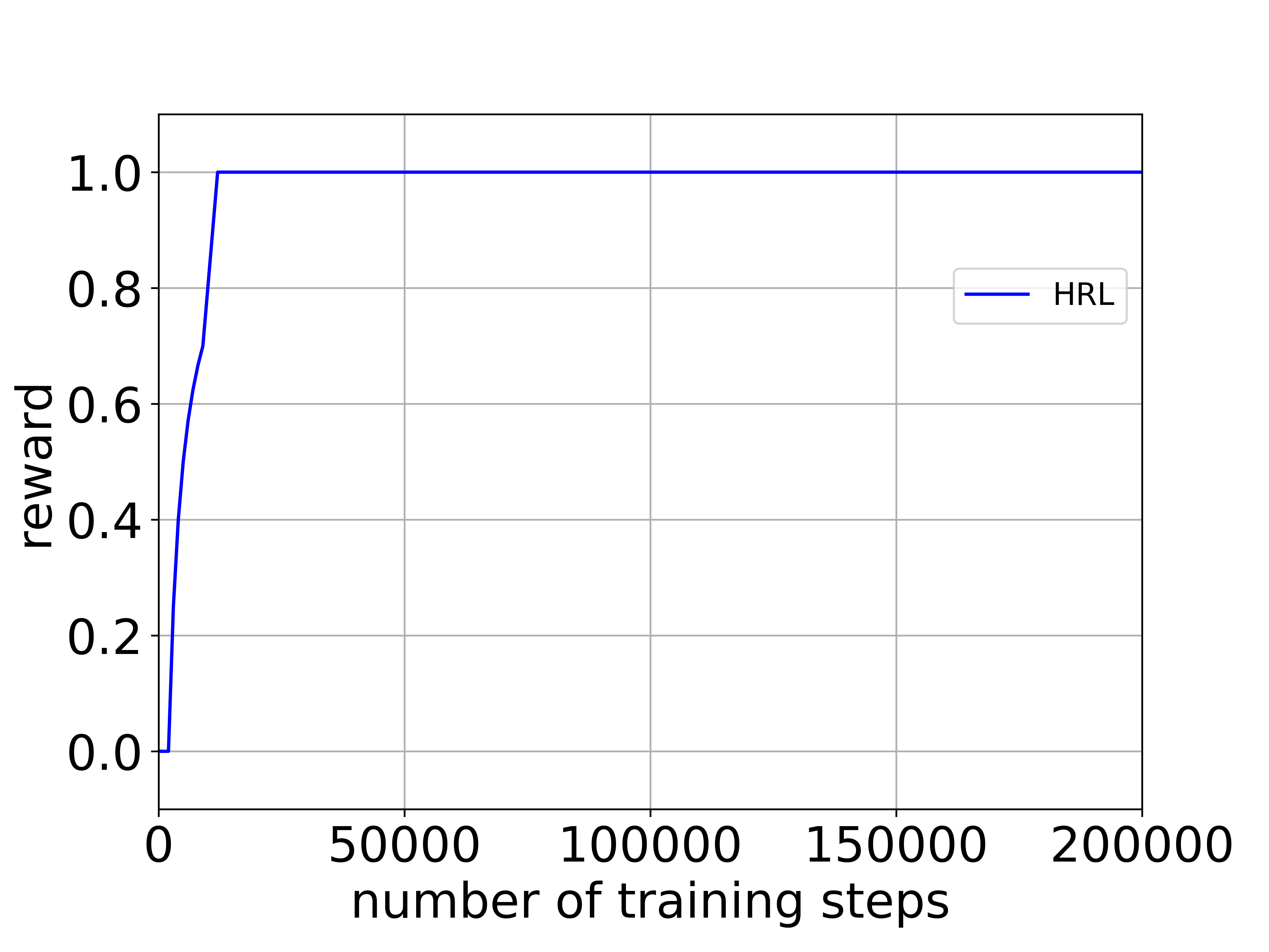
((c))

Figure 9: Cumulative rewards of 10 independent simulation runs averaged for every 10 training steps for task 2.1 in the office world scenario: (a) JIRP; (b) QAS; (c) HRL.

G.2 Task 2.2

For task 2.2, Figure 10 shows the inferred hypothesis reward machine in the last iteration of JIRP. Figure 11 shows the cumulative rewards of 10 independent simulation runs averaged for every 10 training steps for task 2.2.

Figure 10: The inferred hypothesis reward machine for task 2.2  in the last iteration of JIRP.

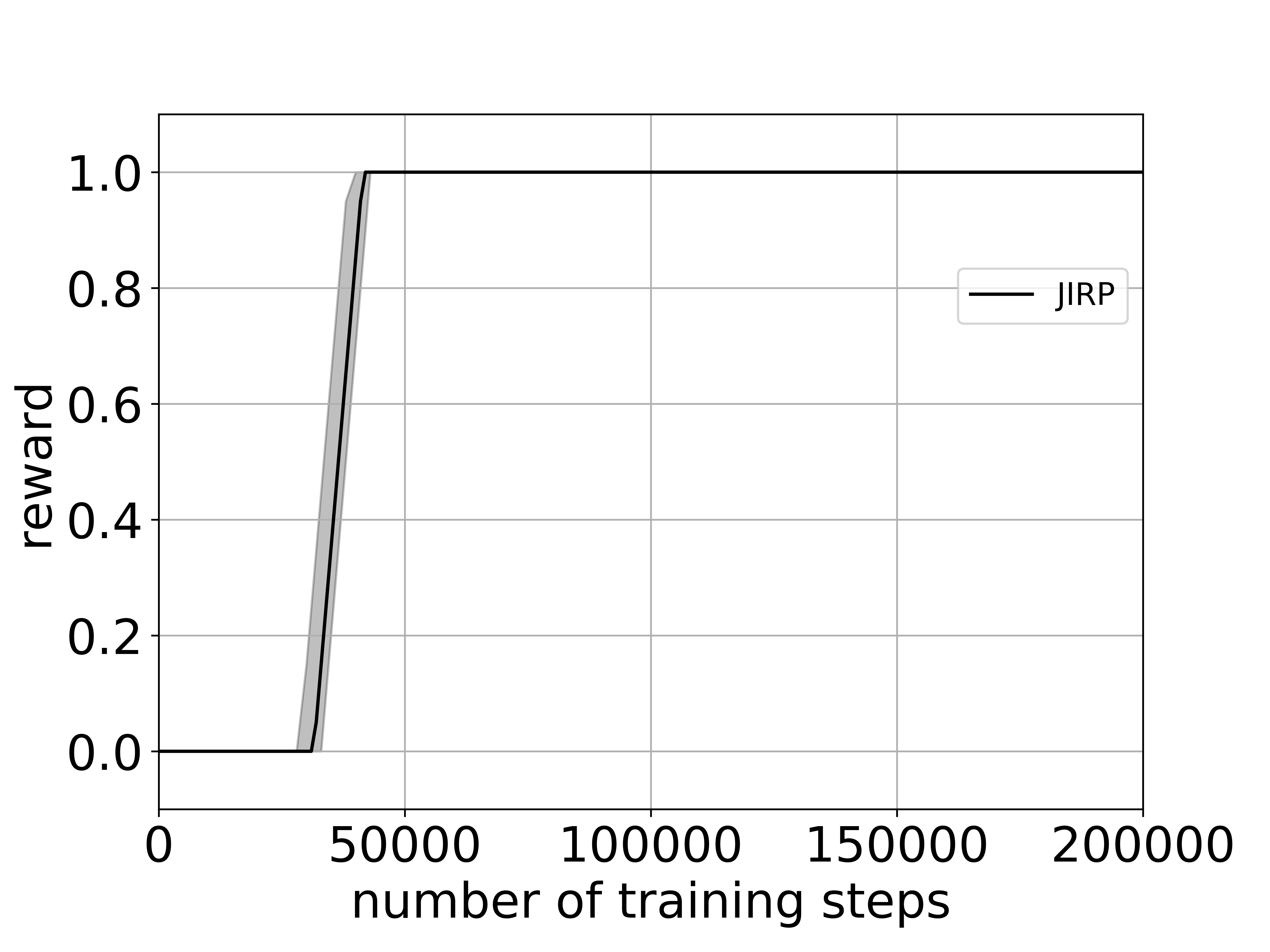
((a))

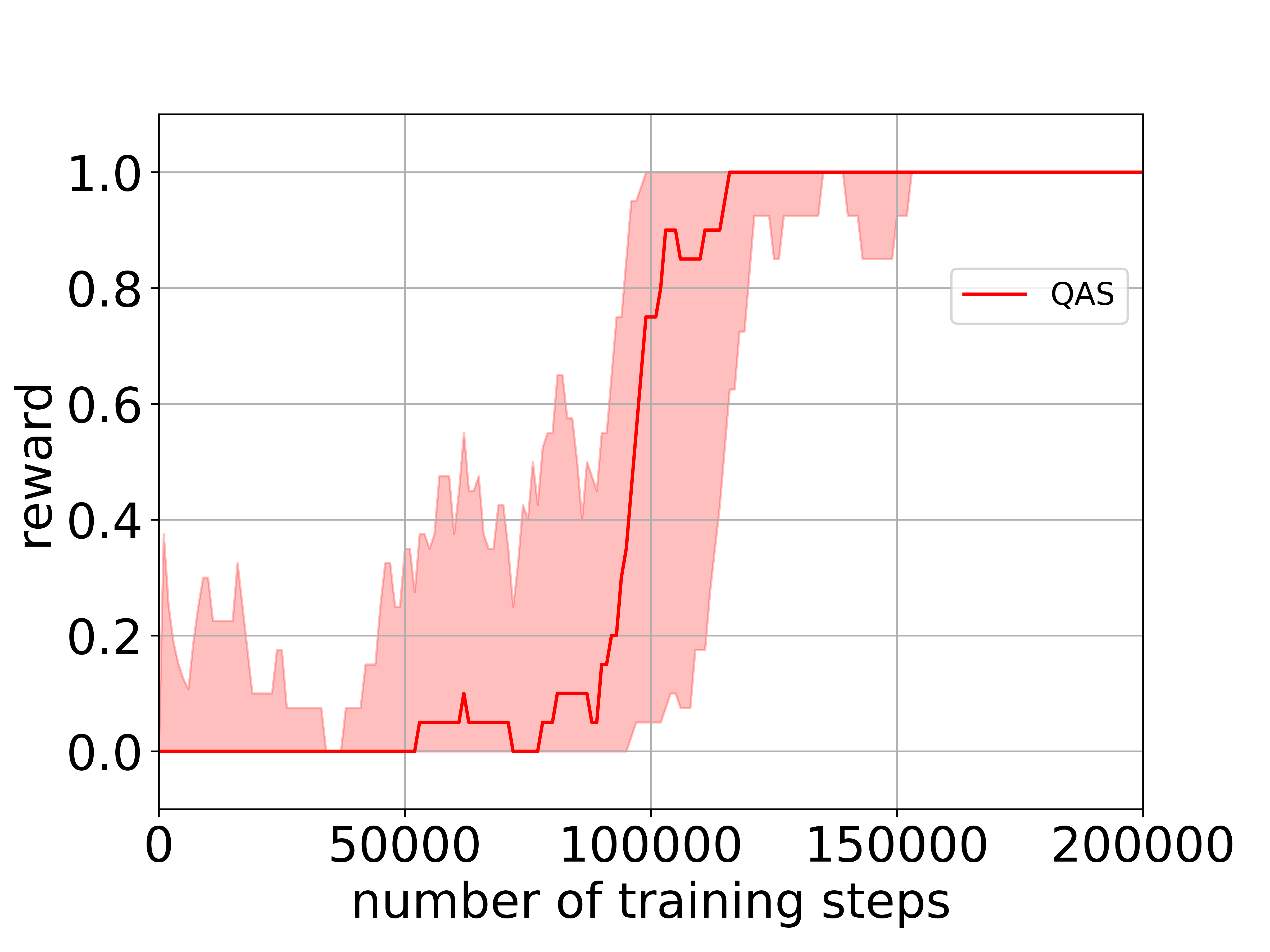
((b))

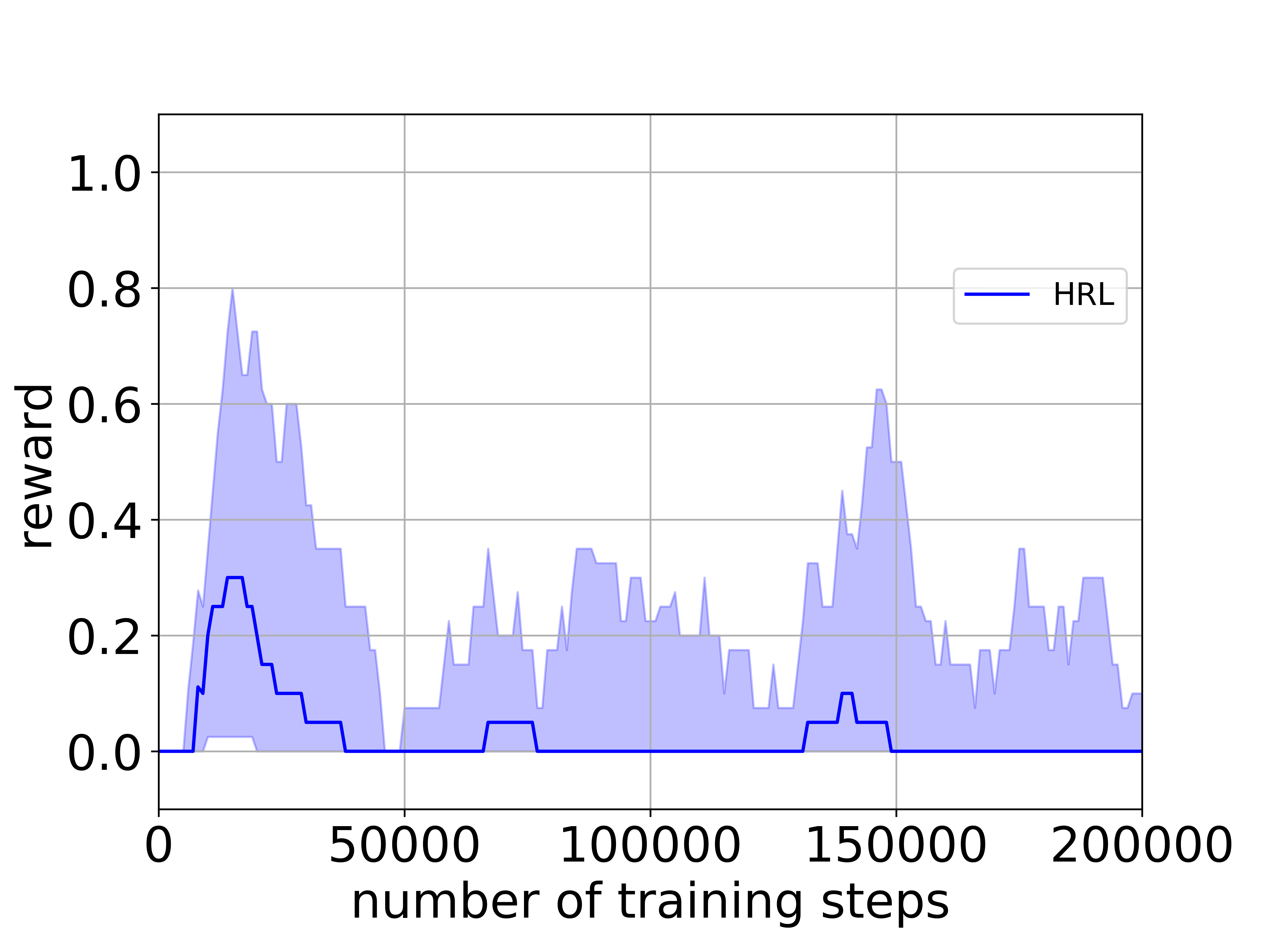
((c))

Figure 11: Cumulative rewards of 10 independent simulation runs averaged for every 10 training steps for task 2.2 in the office world scenario: (a) JIRP; (b) QAS; (c) HRL.

G.3 Task 2.3

For task 2.3, Figure 12 shows the inferred hypothesis reward machine in the last iteration of JIRP. Figure 13 shows the cumulative rewards of 10 independent simulation runs averaged for every 10 training steps for task 2.3.

Figure 12: The inferred hypothesis reward machine for task 2.3 in the last iteration of JIRP.

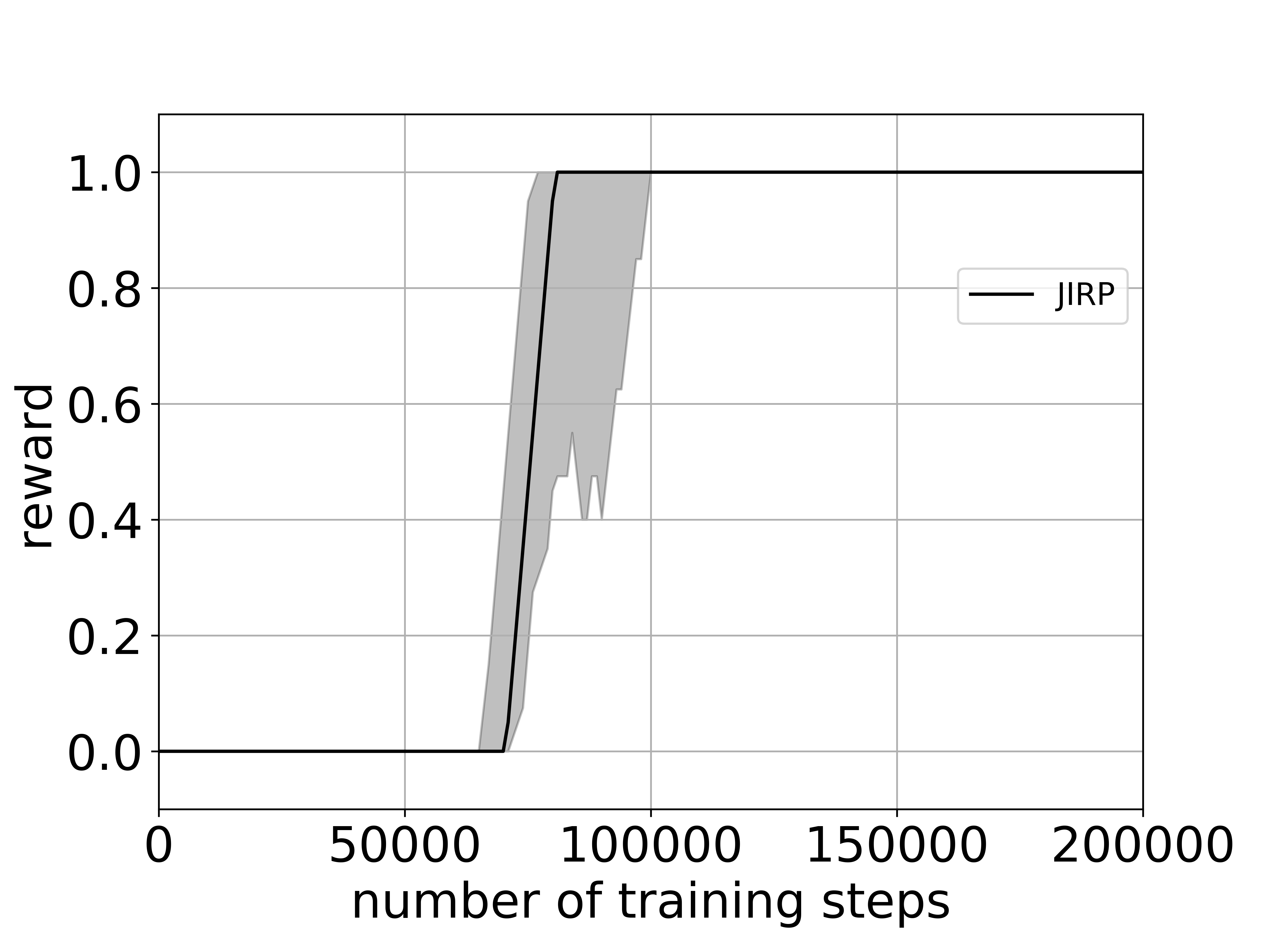
((a))

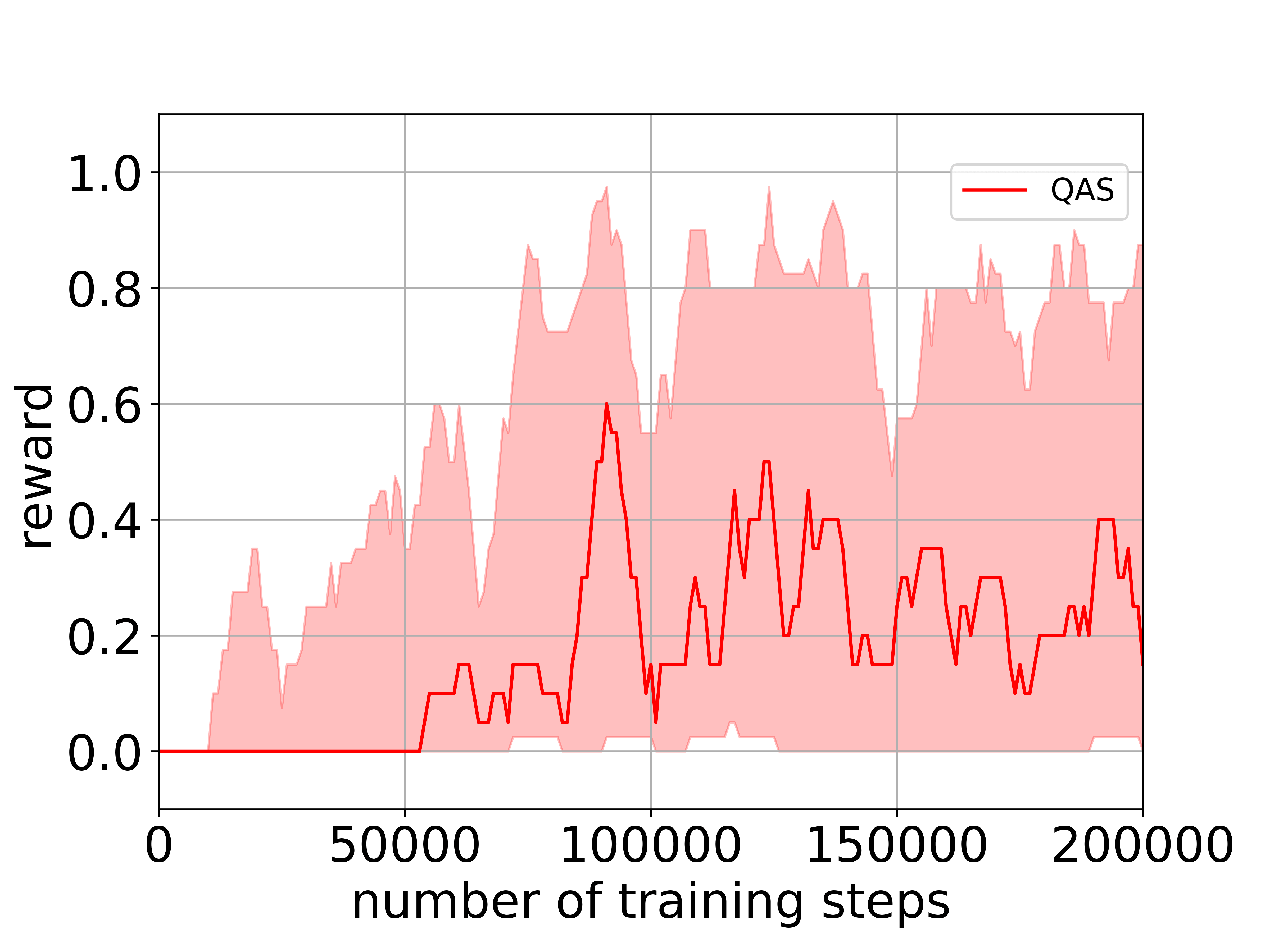
((b))

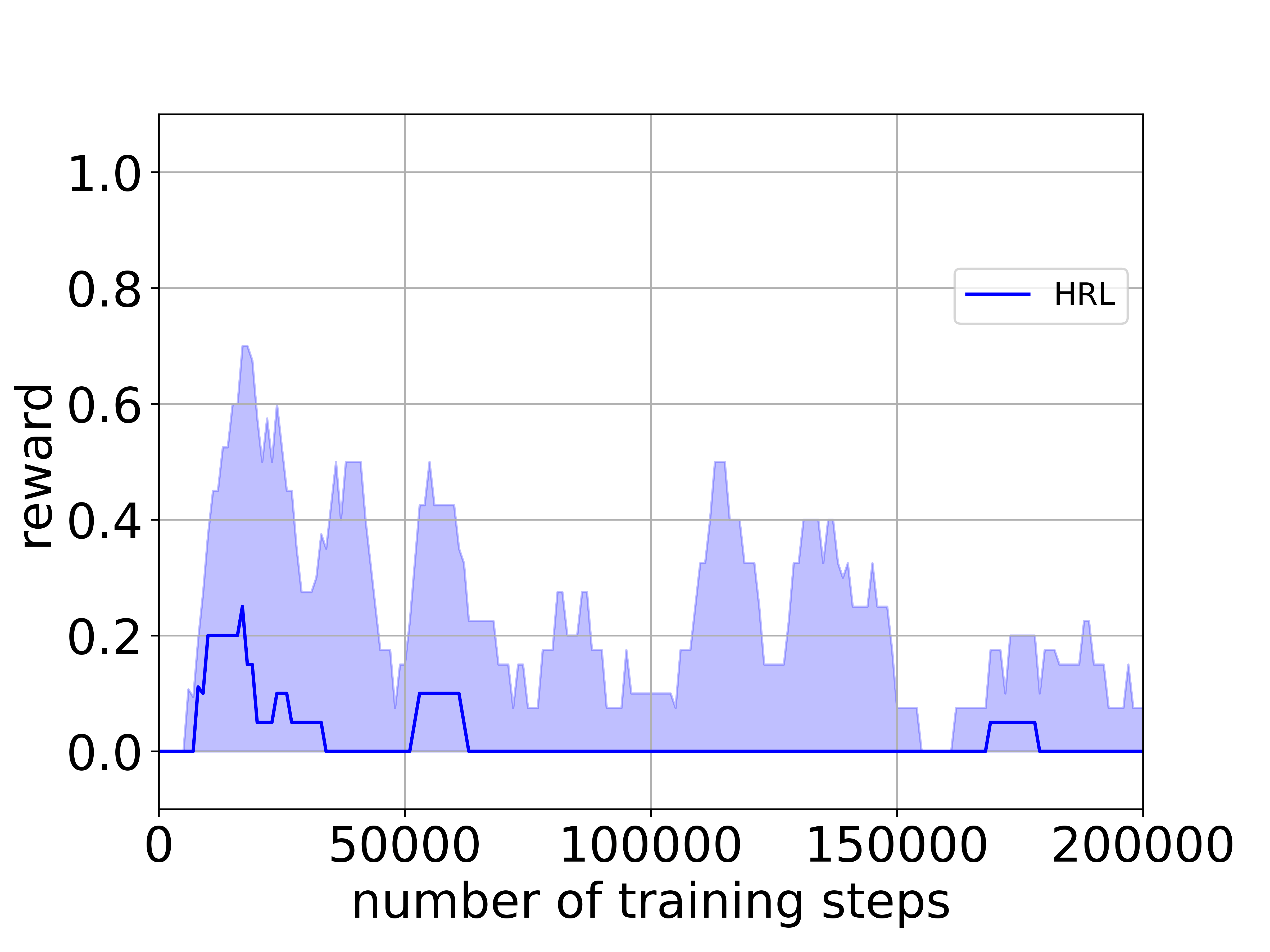
((c))

Figure 13: Cumulative rewards of 10 independent simulation runs averaged for every 10 training steps for task 2.3 in the office world scenario: (a) JIRP; (b) QAS; (c) HRL.

G.4 Task 2.4

For task 2.4, Figure 15 shows the inferred hypothesis reward machine in the last iteration of JIRP. Figure 15 shows the cumulative rewards of 10 independent simulation runs averaged for every 10 training steps for task 2.4.

Figure 14: The inferred hypothesis reward machine for task 2.4 in the last iteration of JIRP.

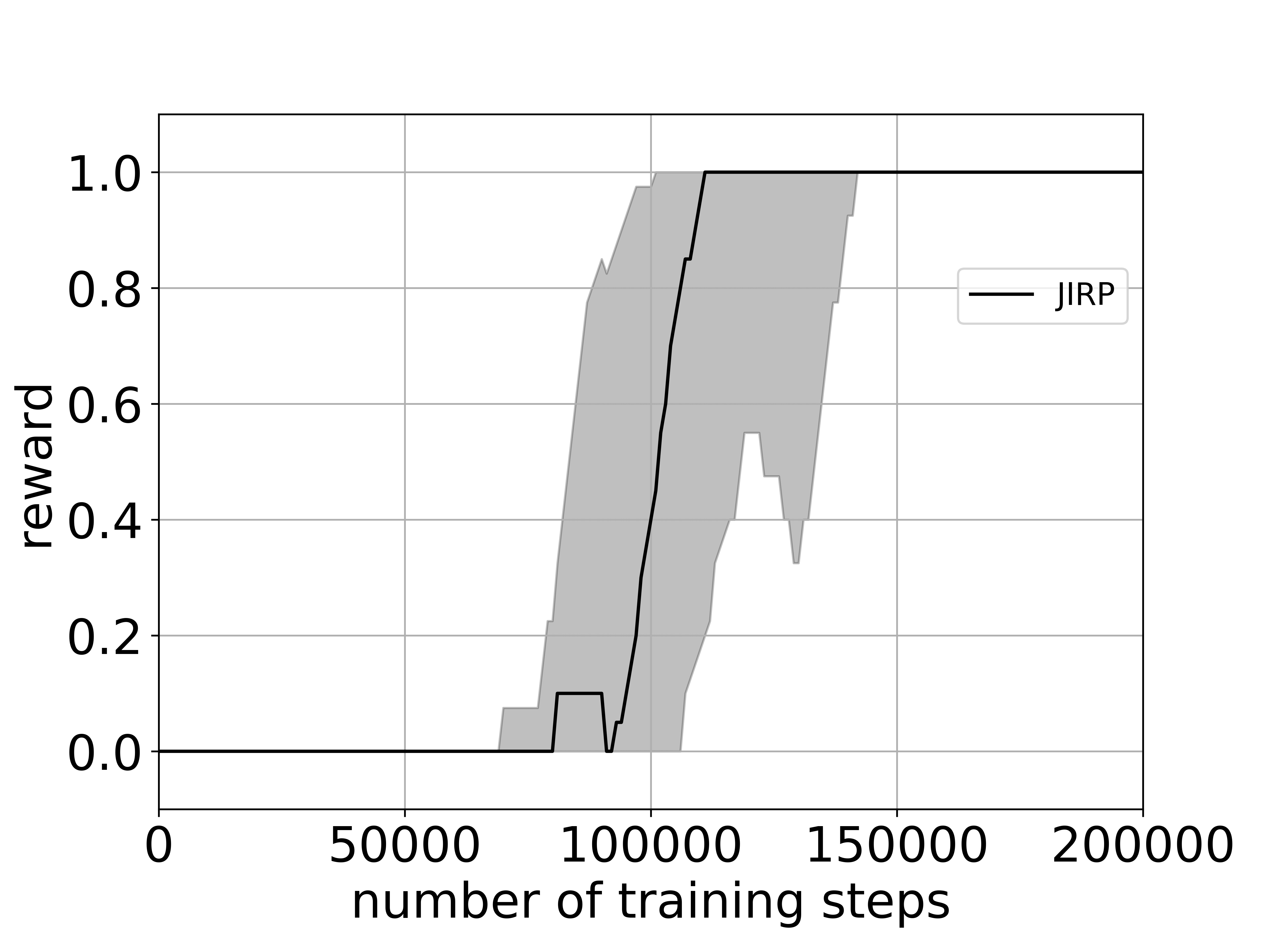
((a))

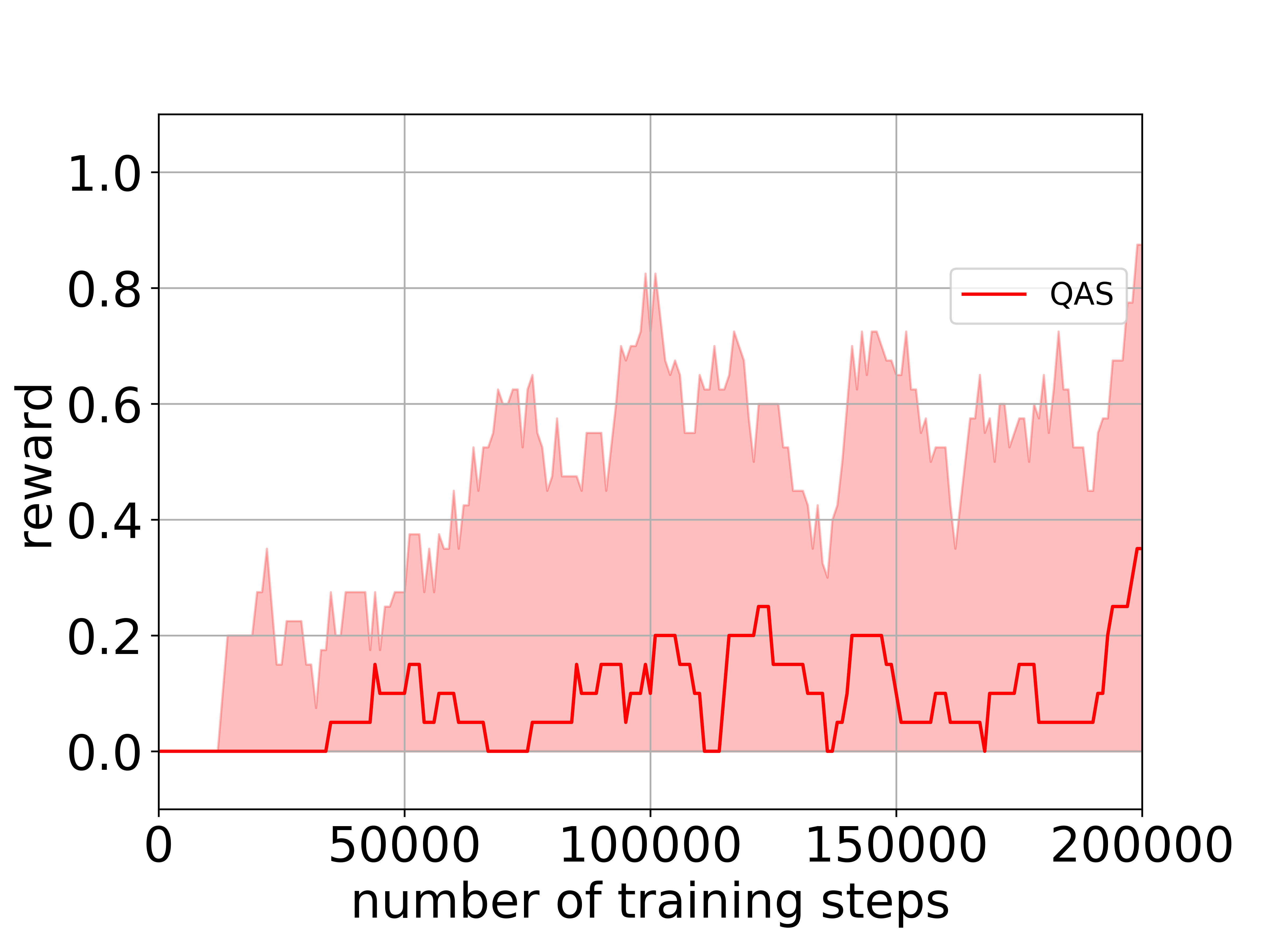
((b))

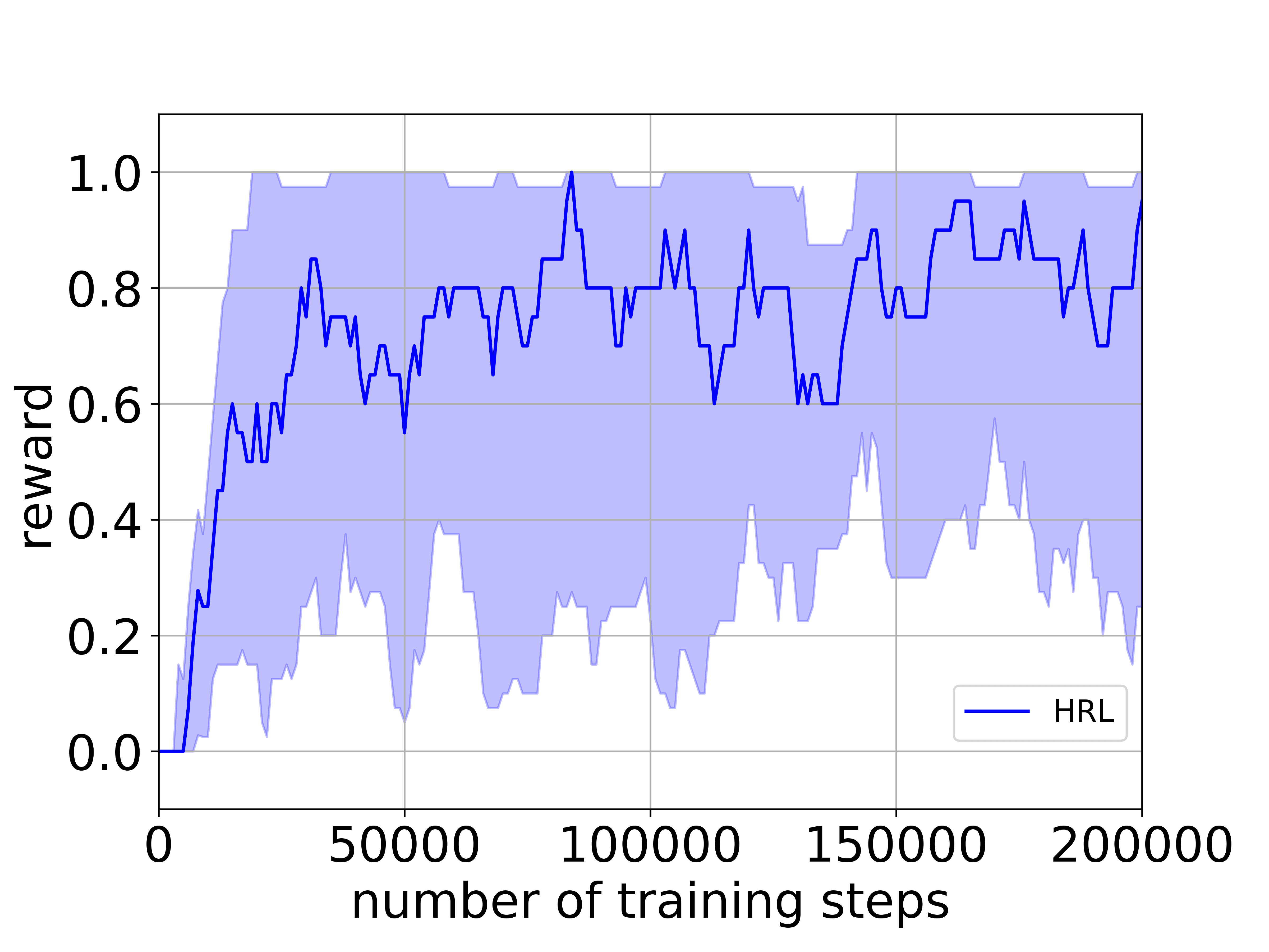
((c))

Figure 15: Cumulative rewards of 10 independent simulation runs averaged for every 10 training steps for task 2.4 in the office world scenario: (a) JIRP; (b) QAS; (c) HRL.

Appendix H Details in Minecraft World Scenario

We provide the detailed results in Minecraft world scenario. Figure 16 shows the map in the office world scenario. We use the triangle to denote the initial position of the agent. We consider the following four tasks:
Task 3.1: make plank: get wood w, then use toolshed t (toolshed cannot be used before wood is gotten);
Task 3.2: make stick: get wood w, then use workbench h (workbench can be used before wood is gotten);
Task 3.3: make bow: go to workbench h, get wood w, then go to workbench h and use factory f (in the listed order);
Task 3.4: make bridge: get wood w, get iron i, then get wood w and use factory f (in the listed order).

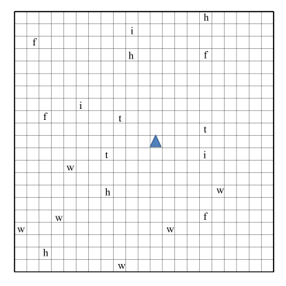
Figure 16: The map in the Minecraft world scenario.

H.1 Task 3.1

For task 3.1, Figure 17 shows the inferred hypothesis reward machine in the last iteration of JIRP. Figure 18 shows the cumulative rewards of 10 independent simulation runs averaged for every 10 training steps for task 3.1.

Figure 17: The inferred hypothesis reward machine for task 3.1  in the last iteration of JIRP.

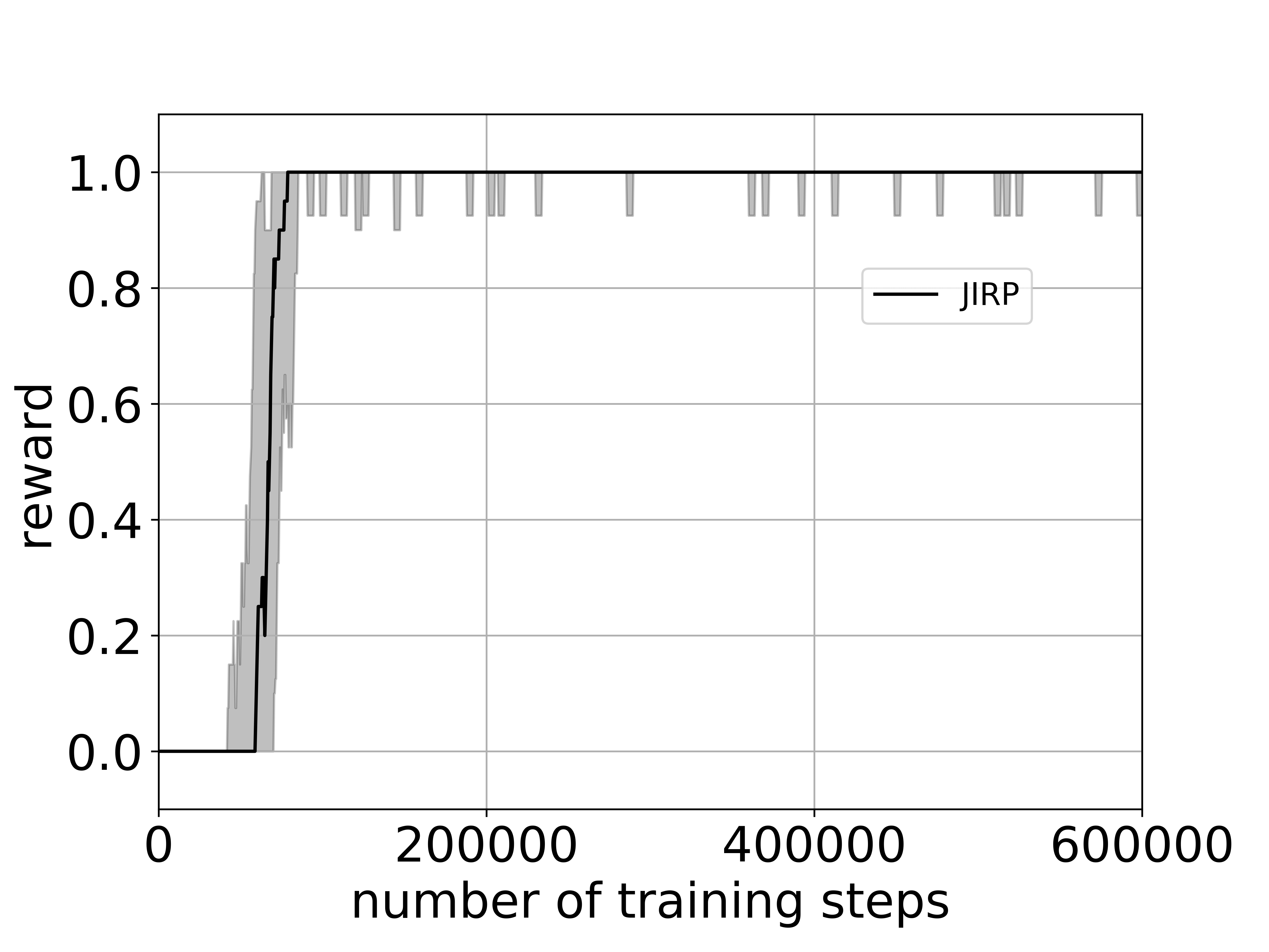
((a))

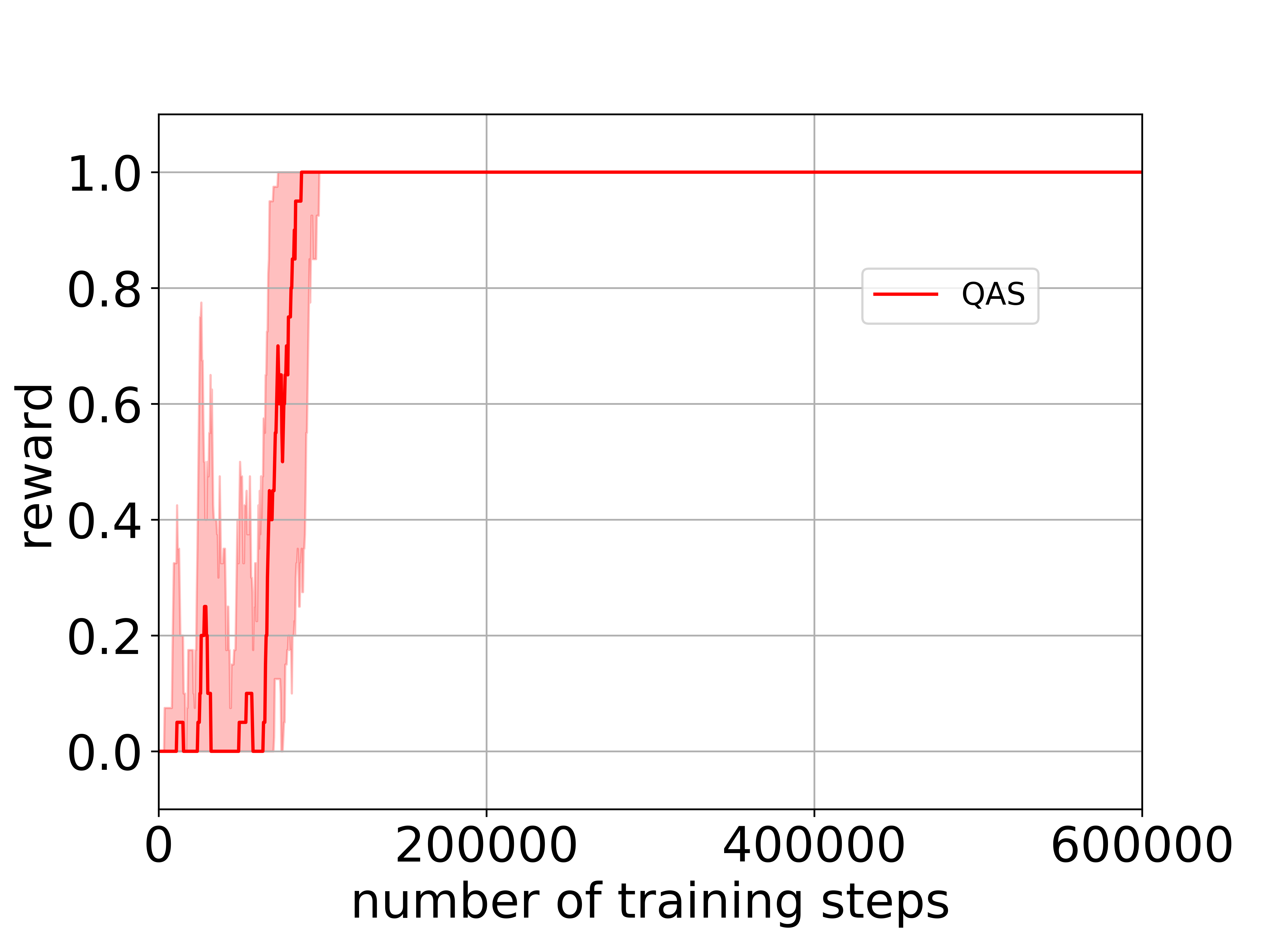
((b))

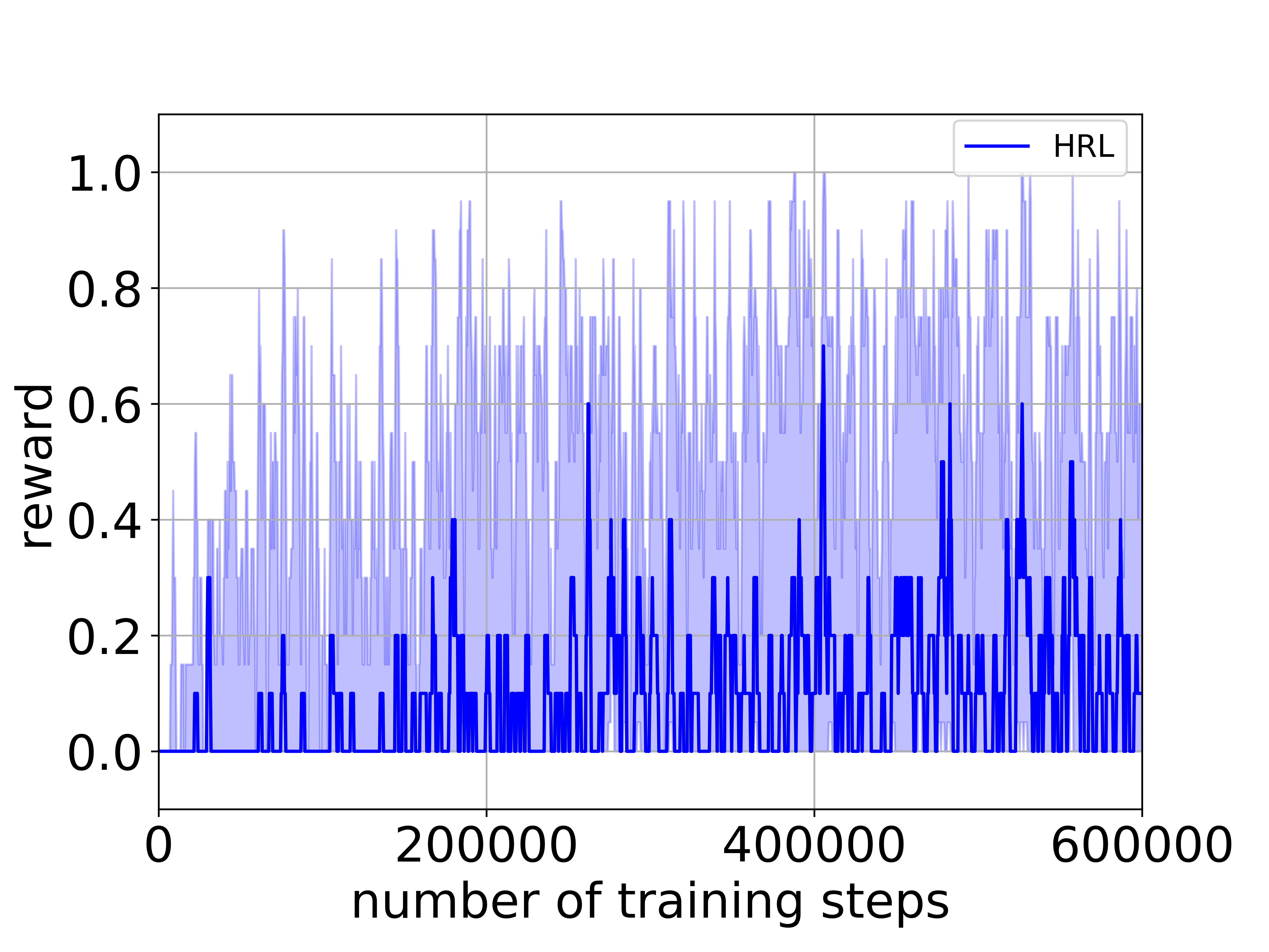
((c))

Figure 18: Cumulative rewards of 10 independent simulation runs averaged for every 10 training steps for task 3.1 in the Minecraft world scenario: (a) JIRP; (b) QAS; (c) HRL.

H.2 Task 3.2

For task 3.2, Figure 19 shows the inferred hypothesis reward machine in the last iteration of JIRP. Figure 20 shows the cumulative rewards of 10 independent simulation runs averaged for every 10 training steps for task 3.2.

Figure 19: The inferred hypothesis reward machine for task 3.2  in the last iteration of JIRP.

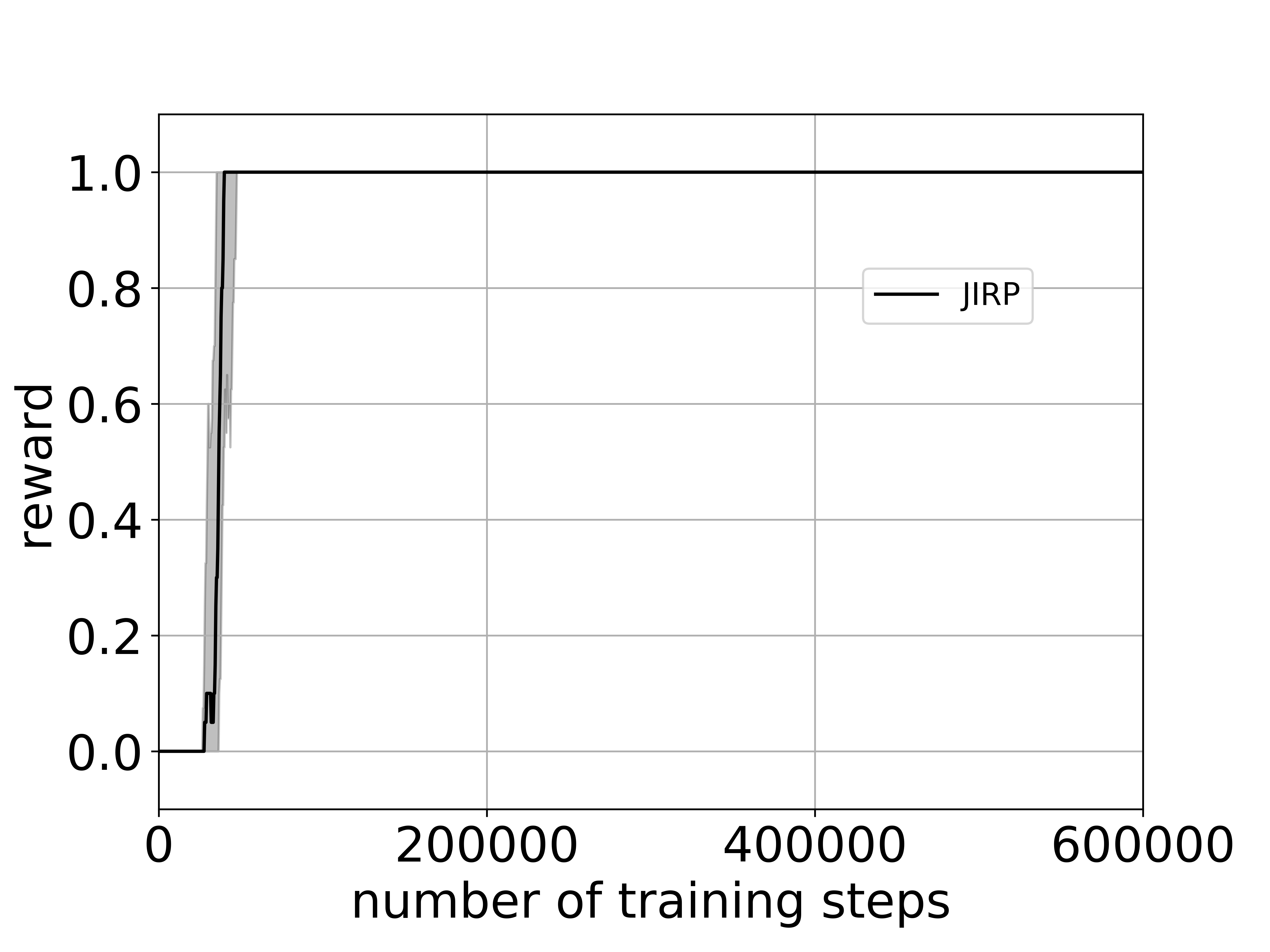
((a))

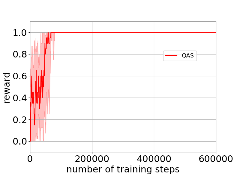
((b))

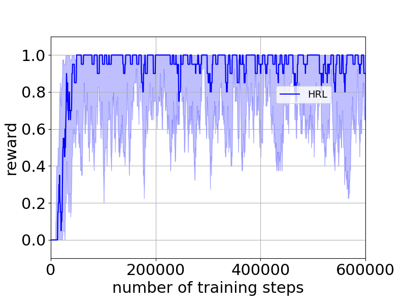
((c))

Figure 20: Cumulative rewards of 10 independent simulation runs averaged for every 10 training steps for task 3.2 in the Minecraft world scenario: (a) JIRP; (b) QAS; (c) HRL.

H.3 Task 3.3

For task 3.3, Figure 21 shows the inferred hypothesis reward machine in the last iteration of JIRP. Figure 22 shows the cumulative rewards of 10 independent simulation runs averaged for every 10 training steps for task 3.3.

Figure 21: The inferred hypothesis reward machine for task 3.3  in the last iteration of JIRP.

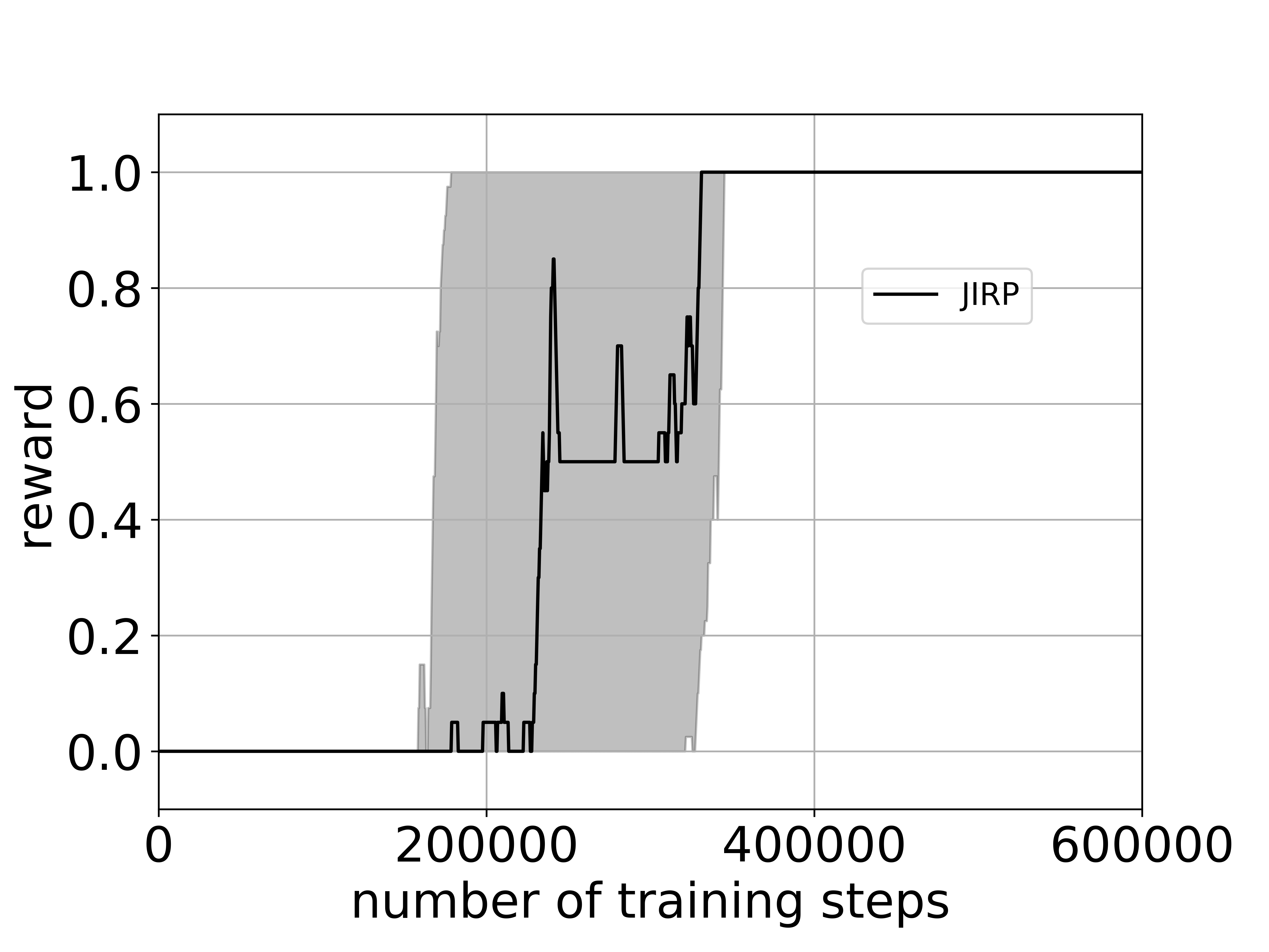
((a))

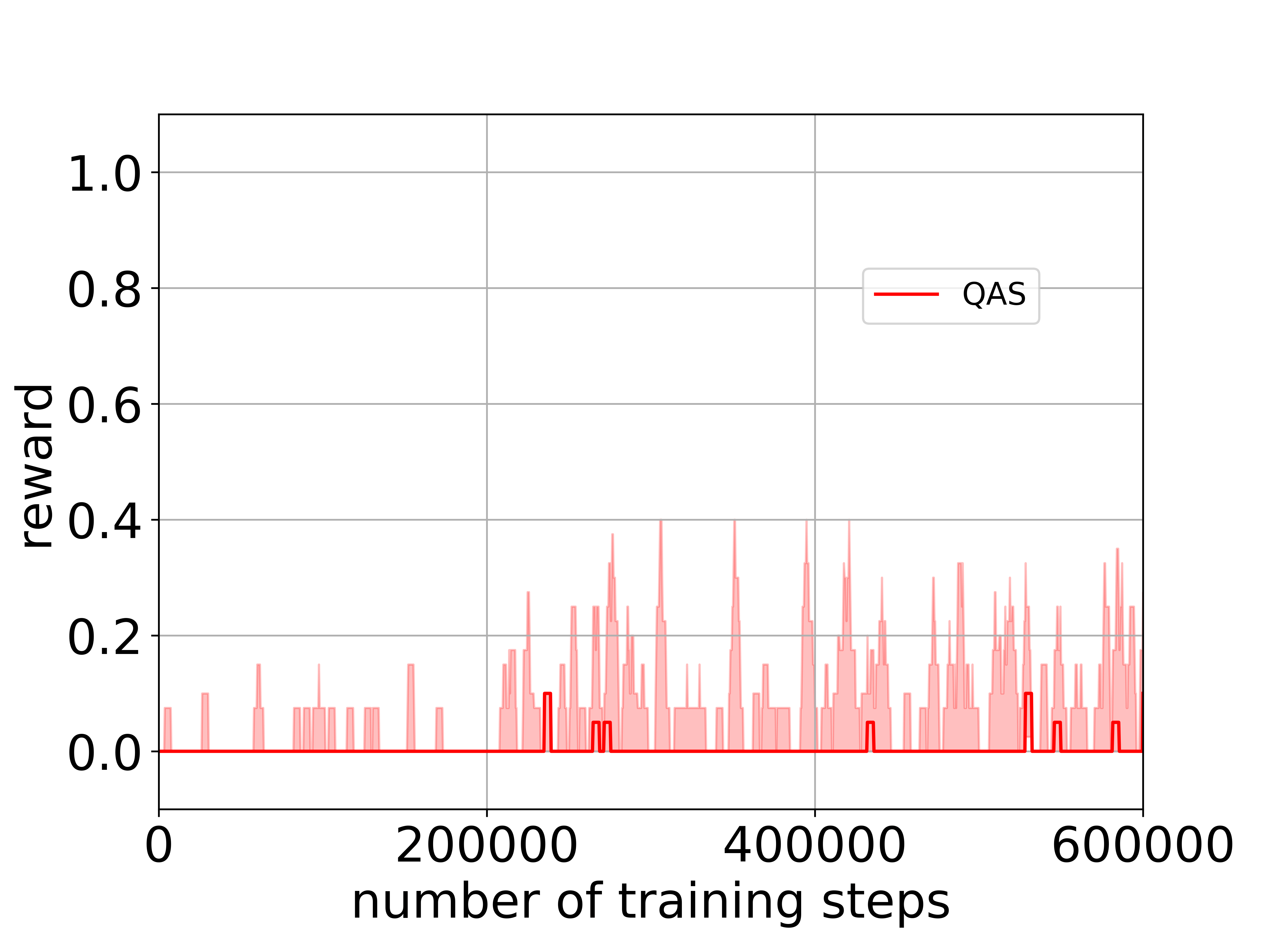
((b))

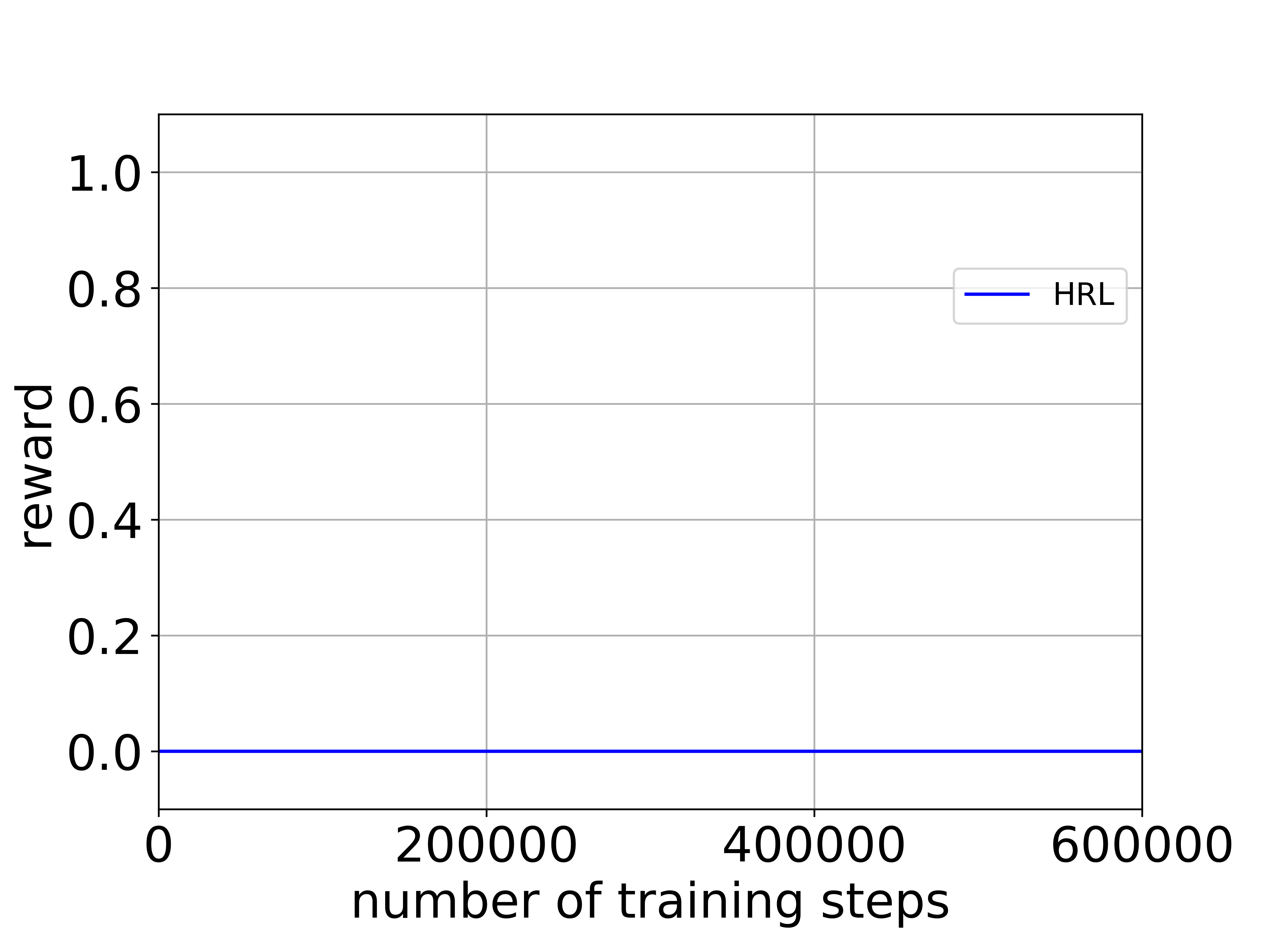
((c))

Figure 22: Cumulative rewards of 10 independent simulation runs averaged for every 10 training steps for task 3.3 in the Minecraft world scenario: (a) JIRP; (b) QAS; (c) HRL.

H.4 Task 3.4

For task 3.4, Figure 23 shows the inferred hypothesis reward machine in the last iteration of JIRP. Figure 24 shows the cumulative rewards of 10 independent simulation runs averaged for every 10 training steps for task 3.4.

Figure 23: The inferred hypothesis reward machine for task 3.4  in the last iteration of JIRP.

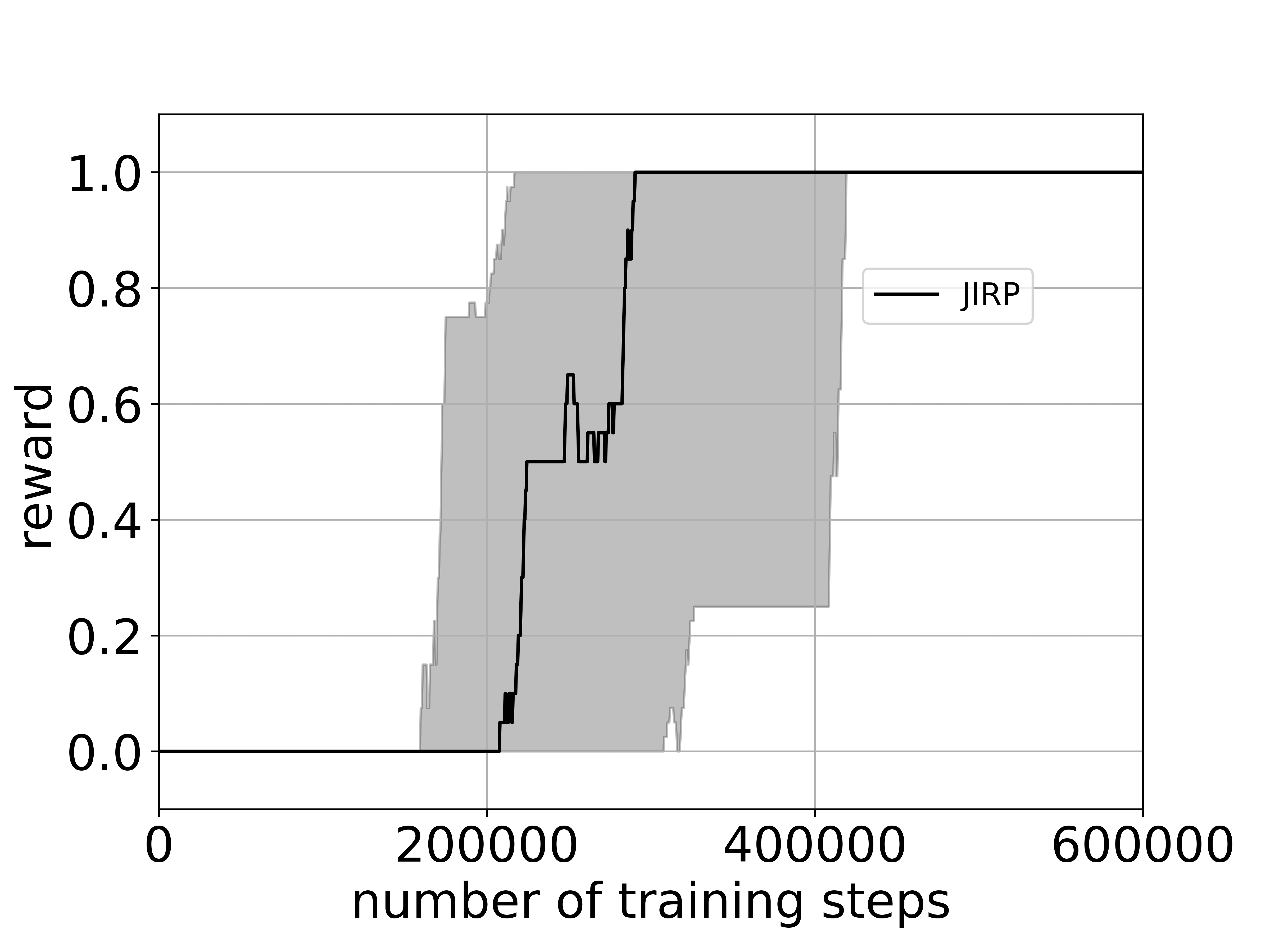
((a))

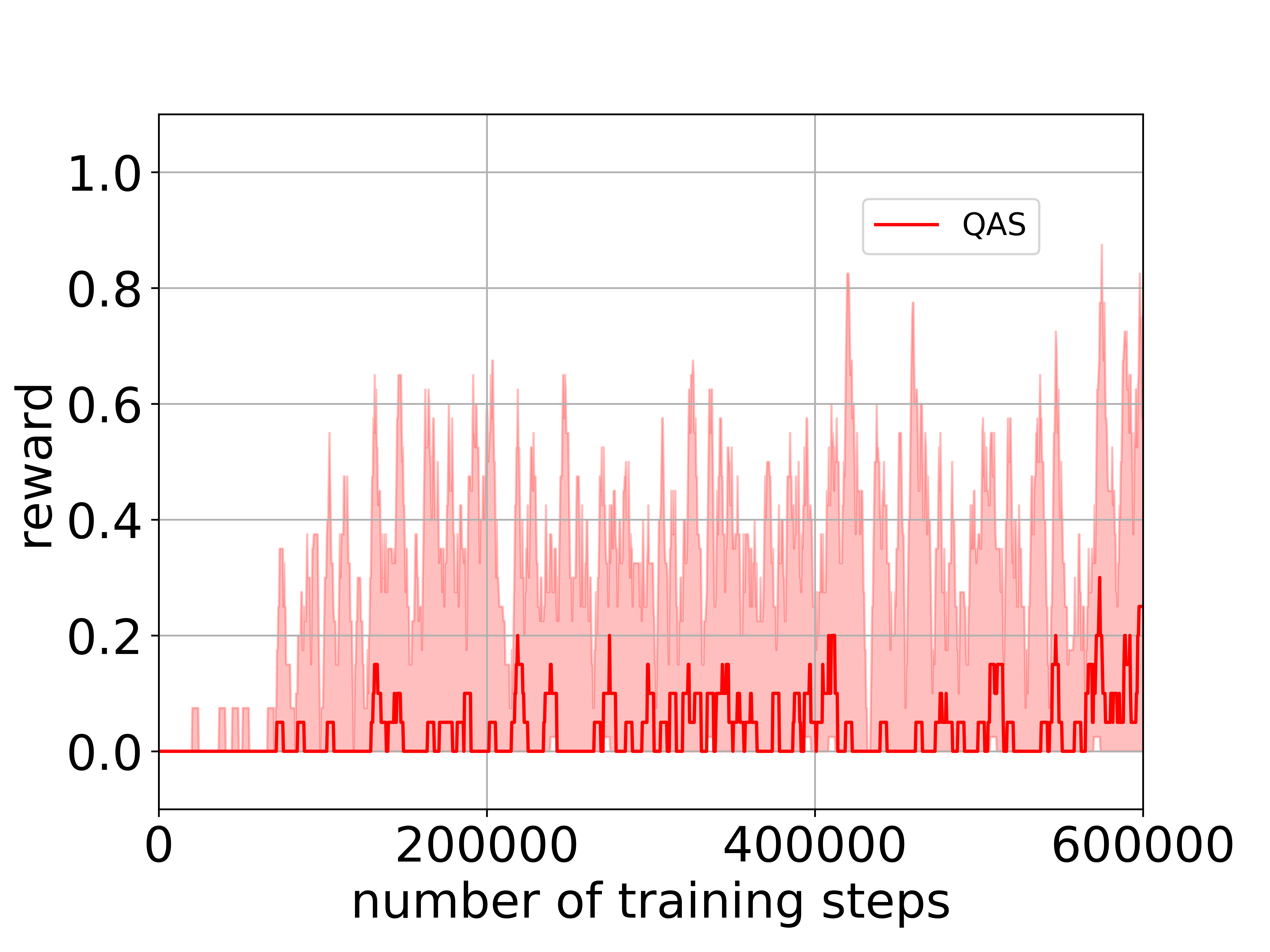
((b))

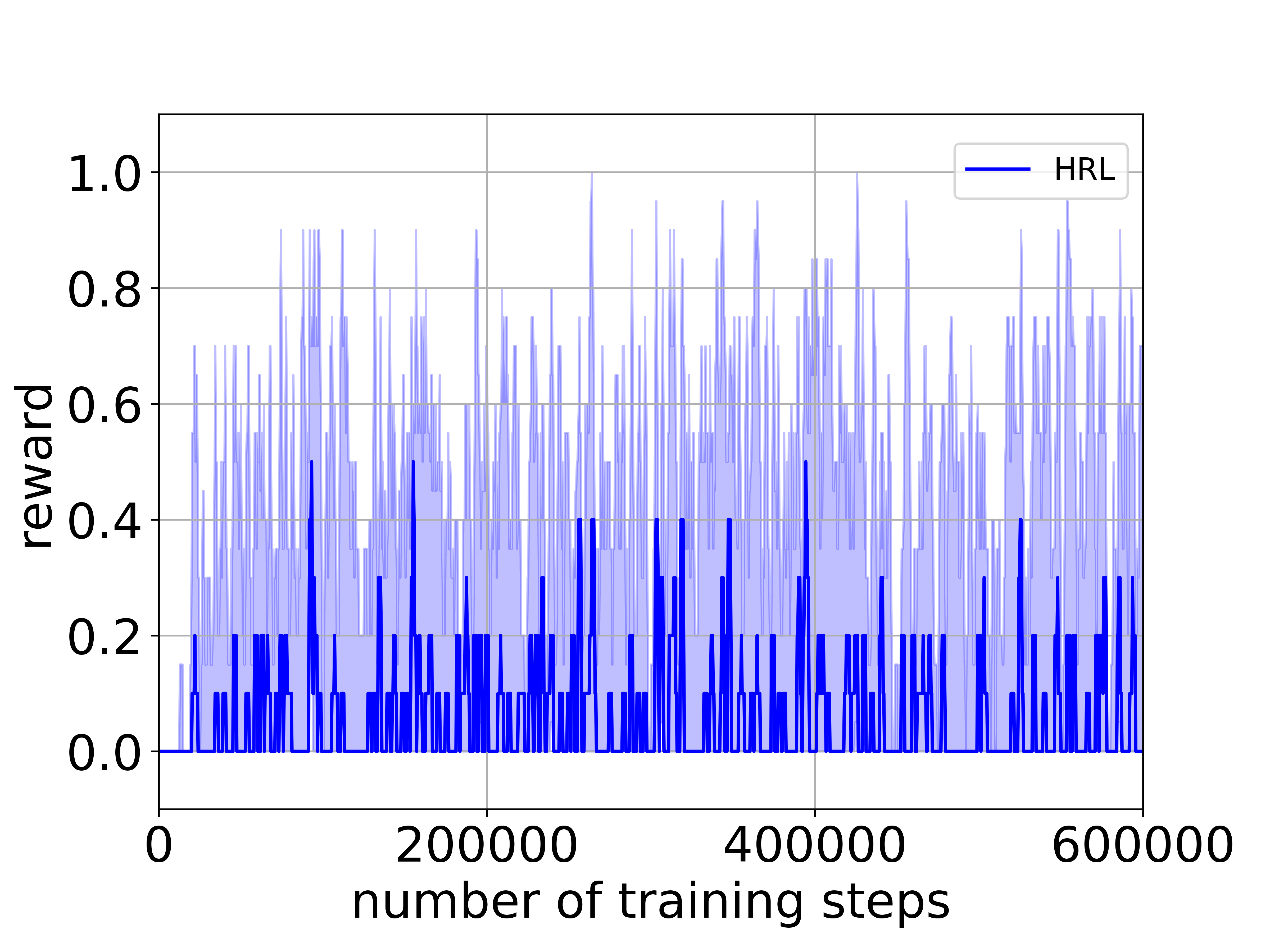
((c))

Figure 24: Cumulative rewards of 10 independent simulation runs averaged for every 10 training steps for task 3.4 in the Minecraft world scenario: (a) JIRP; (b) QAS; (c) HRL.

References

- [1] M. E. Taylor and P. Stone, “Cross-domain transfer for reinforcement learning,” in Proc. ICML’07. New York, NY, USA: ACM, 2007, pp. 879–886. [Online]. Available: http://doi.acm.org/10.1145/1273496.1273607
- [2] O. Nachum, S. S. Gu, H. Lee, and S. Levine, “Data-efficient hierarchical reinforcement learning,” in Advances in Neural Information Processing Systems 31, S. Bengio, H. Wallach, H. Larochelle, K. Grauman, N. Cesa-Bianchi, and R. Garnett, Eds. Curran Associates, Inc., 2018, pp. 3303–3313. [Online]. Available: http://papers.nips.cc/paper/7591-data-efficient-hierarchical-reinforcement-learning.pdf
- [3] D. Abel, D. Arumugam, L. Lehnert, and M. Littman, “State abstractions for lifelong reinforcement learning,” in Proceedings of the 35th International Conference on Machine Learning, ser. Proceedings of Machine Learning Research, J. Dy and A. Krause, Eds., vol. 80. Stockholmsmässan, Stockholm Sweden: PMLR, 10–15 Jul 2018, pp. 10–19. [Online]. Available: http://proceedings.mlr.press/v80/abel18a.html
- [4] R. Akrour, F. Veiga, J. Peters, and G. Neumann, “Regularizing reinforcement learning with state abstraction,” 10 2018, pp. 534–539.
- [5] R. S. Sutton, D. Precup, and S. Singh, “Between mdps and semi-mdps: A framework for temporal abstraction in reinforcement learning,” Artificial intelligence, vol. 112, no. 1-2, pp. 181–211, 1999.
- [6] T. G. Dietterich, “Hierarchical reinforcement learning with the maxq value function decomposition,” J. Artif. Int. Res., vol. 13, no. 1, pp. 227–303, Nov. 2000. [Online]. Available: http://dl.acm.org/citation.cfm?id=1622262.1622268
- [7] R. Parr and S. J. Russell, “Reinforcement learning with hierarchies of machines,” in Advances in neural information processing systems, 1998, pp. 1043–1049.
- [8] A. G. Barto and S. Mahadevan, “Recent advances in hierarchical reinforcement learning,” Discrete event dynamic systems, vol. 13, no. 1-2, pp. 41–77, 2003.
- [9] D. Aksaray, A. Jones, Z. Kong, M. Schwager, and C. Belta, “Q-learning for robust satisfaction of signal temporal logic specifications,” in 2016 IEEE 55th Conference on Decision and Control (CDC). IEEE, 2016, pp. 6565–6570.
- [10] J. Andreas, D. Klein, and S. Levine, “Modular multitask reinforcement learning with policy sketches,” in Proceedings of the 34th International Conference on Machine Learning-Volume 70. JMLR. org, 2017, pp. 166–175.
- [11] X. Li, C.-I. Vasile, and C. Belta, “Reinforcement learning with temporal logic rewards,” in 2017 IEEE/RSJ International Conference on Intelligent Robots and Systems (IROS). IEEE, 2017, pp. 3834–3839.
- [12] Z. Xu and U. Topcu, “Transfer of temporal logic formulas in reinforcement learning,” in IJCAI-19. International Joint Conferences on Artificial Intelligence Organization, 7 2019, pp. 4010–4018. [Online]. Available: https://doi.org/10.24963/ijcai.2019/557
- [13] R. T. Icarte, T. Q. Klassen, R. A. Valenzano, and S. A. McIlraith, “Using reward machines for high-level task specification and decomposition in reinforcement learning,” in Proceedings of the 35th International Conference on Machine Learning, ICML 2018, Stockholmsmässan, Stockholm, Sweden, July 10-15, 2018, 2018, pp. 2112–2121. [Online]. Available: http://proceedings.mlr.press/v80/icarte18a.html
- [14] C. J. C. H. Watkins and P. Dayan, “Q-learning,” Machine Learning, vol. 8, no. 3, pp. 279–292, May 1992. [Online]. Available: https://doi.org/10.1007/BF00992698
- [15] D. Neider and N. Jansen, “Regular model checking using solver technologies and automata learning,” in NASA Formal Methods, 5th International Symposium, NFM 2013, Moffett Field, CA, USA, May 14-16, 2013. Proceedings, ser. Lecture Notes in Computer Science, vol. 7871. Springer, 2013, pp. 16–31.
- [16] J. Oncina and P. Garcia, “Inferring regular languages in polynomial updated time,” in Pattern recognition and image analysis: selected papers from the IVth Spanish Symposium. World Scientific, 1992, pp. 49–61.
- [17] T. D. Kulkarni, K. Narasimhan, A. Saeedi, and J. Tenenbaum, “Hierarchical deep reinforcement learning: Integrating temporal abstraction and intrinsic motivation,” in Advances in neural information processing systems, 2016, pp. 3675–3683.
- [18] M. L. Puterman, Markov Decision Processes: Discrete Stochastic Dynamic Programming, 1st ed. New York, NY, USA: John Wiley & Sons, Inc., 1994.
- [19] A. Camacho, R. Toro Icarte, T. Q. Klassen, R. Valenzano, and S. A. McIlraith, “LTL and beyond: Formal languages for reward function specification in reinforcement learning,” in IJCAI’19. International Joint Conferences on Artificial Intelligence Organization, 7 2019, pp. 6065–6073. [Online]. Available: https://doi.org/10.24963/ijcai.2019/840
- [20] J. O. Shallit, A Second Course in Formal Languages and Automata Theory. Cambridge University Press, 2008. [Online]. Available: http://www.cambridge.org/gb/knowledge/isbn/item1173872/?site_locale=en_GB
- [21] R. S. Sutton and A. G. Barto, Reinforcement learning: An introduction. MIT press, 2018.
- [22] D. Angluin, “Learning regular sets from queries and counterexamples,” Inf. Comput., vol. 75, no. 2, pp. 87–106, 1987. [Online]. Available: https://doi.org/10.1016/0890-5401(87)90052-6
- [23] C. Löding, P. Madhusudan, and D. Neider, “Abstract learning frameworks for synthesis,” in Tools and Algorithms for the Construction and Analysis of Systems - 22nd International Conference, TACAS 2016, Held as Part of the European Joint Conferences on Theory and Practice of Software, ETAPS 2016, Eindhoven, The Netherlands, April 2-8, 2016, Proceedings, ser. Lecture Notes in Computer Science, vol. 9636. Springer, 2016, pp. 167–185.
- [24] E. M. Gold, “Complexity of automaton identification from given data,” Information and Control, vol. 37, no. 3, pp. 302–320, 1978.
- [25] M. Heule and S. Verwer, “Exact DFA identification using SAT solvers,” in Grammatical Inference: Theoretical Results and Applications, 10th International Colloquium, ICGI 2010, Valencia, Spain, September 13-16, 2010. Proceedings, ser. Lecture Notes in Computer Science, vol. 6339. Springer, 2010, pp. 66–79.
- [26] D. Neider, “Applications of automata learning in verification and synthesis,” Ph.D. dissertation, RWTH Aachen University, 2014. [Online]. Available: http://darwin.bth.rwth-aachen.de/opus3/volltexte/2014/5169
- [27] B. Bollig, J. Katoen, C. Kern, M. Leucker, D. Neider, and D. R. Piegdon, “libalf: The automata learning framework,” in Computer Aided Verification, 22nd International Conference, CAV 2010, Edinburgh, UK, July 15-19, 2010. Proceedings, 2010, pp. 360–364. [Online]. Available: https://doi.org/10.1007/978-3-642-14295-6_32
- [28] R. Givan, T. Dean, and M. Greig, “Equivalence notions and model minimization in markov decision processes,” Artificial Intelligence, vol. 147, no. 1, pp. 163 – 223, 2003, planning with Uncertainty and Incomplete Information. [Online]. Available: http://www.sciencedirect.com/science/article/pii/S0004370202003764