Data compression in cosmology: A compressed likelihood for Planck data

Abstract

We apply the Massively Optimized Parameter Estimation and Data compression technique (MOPED) to the public Planck 2015 temperature likelihood, reducing the dimensions of the data space to one number per parameter of interest. We present CosMOPED, a lightweight and convenient compressed likelihood code implemented in Python. In doing so we show that the $\ell<30$ Planck temperature likelihood can be well approximated by two Gaussian distributed data points, which allows us to replace the map-based low-$\ell$ temperature likelihood by a simple Gaussian likelihood. We make available a Python implementation of Planck’s 2015 Plik_lite temperature likelihood that includes these low-$\ell$ binned temperature data (Planck-lite-py). We do not explicitly use the large-scale polarization data in CosMOPED, instead imposing a prior on the optical depth to reionization derived from these data. We show that the $\Lambda$CDM parameters recovered with CosMOPED are consistent with the uncompressed likelihood to within 0.1$\sigma$, and test that a 7-parameter extended model performs similarly well.

I Introduction

When analyzing a large dataset with many different data points, but only a few relevant parameters, it can be useful to compress the data, retaining all the information that is relevant to the parameters of interest. These compressed data can then be used for parameter inference. Tegmark et al. (1997) showed that if there is one parameter of interest, a dataset can be compressed to one number without losing any information about that parameter. The Massively Optimized Parameter Estimation and Data compression technique (MOPED) described in Heavens et al. (2000) extends this to multiple parameters, developing optimal linear compression for Gaussian data provided the covariance is independent of the parameters. Alsing and Wandelt (2018) show that compression to the score function (the gradient of the log likelihood) preserves the information content even for non-Gaussian data and data for which the covariance depends on the parameters. Thus the full dataset of $N$ data points can be compressed to $n$ numbers, where $n$ is the number of parameters of interest, while preserving the Fisher information about those parameters.

This compression step is useful both as a way to generate a simplified likelihood function, and as a step towards likelihood-free inference when the form of the likelihood is not known precisely (e.g., Alsing and Wandelt, 2018). Compressions of this form have been used to study the star formation history of galaxies (Reichardt et al., 2001; Heavens et al., 2004; Panter et al., 2007) and considered for exoplanet transit detections (Protopapas et al., 2005), gravitational wave studies with LISA (Graff et al., 2011), and covariance matrix estimation (Heavens et al., 2017). Gupta and Heavens (2002) proposed applying MOPED compression to cosmic microwave background (CMB) data, and Zablocki and Dodelson (2016) applied a similar compression scheme to the temperature power spectrum of WMAP.

In this paper we apply the MOPED compression to the Planck CMB power spectrum Planck Collaboration (2016a), and show that the standard $\Lambda$CDM  cosmological parameter constraints can be derived from a compressed likelihood of just six Gaussian-distributed data points. We go beyond earlier analyses of CMB data by precompressing the non-Gaussian large-scale temperature power spectrum into two approximately Gaussian data points. We make the software for the MOPED-compressed likelihood publicly available, as well as for the likelihood computed directly from the binned power spectrum with the inclusion of new large angular scale bins.

The outline of the paper is as follows. In §II we describe the public Planck likelihood and the precompression we implement to better approximate it as Gaussian. In §III we describe the MOPED compression scheme we apply, and in §IV show parameter constraints for the $\Lambda$CDM  model and an example extended model with running of the primordial spectral index. We conclude in §V.

II Planck likelihood and low-$\ell$ binning

The current state-of-the-art CMB data come from the Planck satellite. The latest cosmological analysis is reported in Planck Collaboration (2018), with public data from the earlier 2015 analysis described in Planck Collaboration (2016a). The Planck temperature power spectrum is shown in Fig. 1. The likelihood function, describing the probability of the data given some model, is separated into two main parts for the Planck power spectrum analysis, with different approaches for large scales and smaller scales. We summarize these components briefly here.

Figure 1: The Planck 2015 temperature power spectrum from (Planck Collaboration, 2016a). The non-Gaussian $\ell<30$ bandpowers are shown with their asymmetrical errors in gray. The two black points at $\ell<30$ are obtained by estimating the binned spectrum in two angular bins, and have approximately Gaussian distributions. We use these two low-$\ell$ bins for the likelihoods described in this paper. The $\ell\geq 30$ binned data are the foreground-marginalized temperature bandpowers from the Plik_lite likelihood for Planck 2015. The theoretical power spectrum for the Planck 2015 TT+lowTEB best fit parameters (Planck Collaboration, 2016b) computed using CLASS (Blas et al., 2011) is shown in blue.

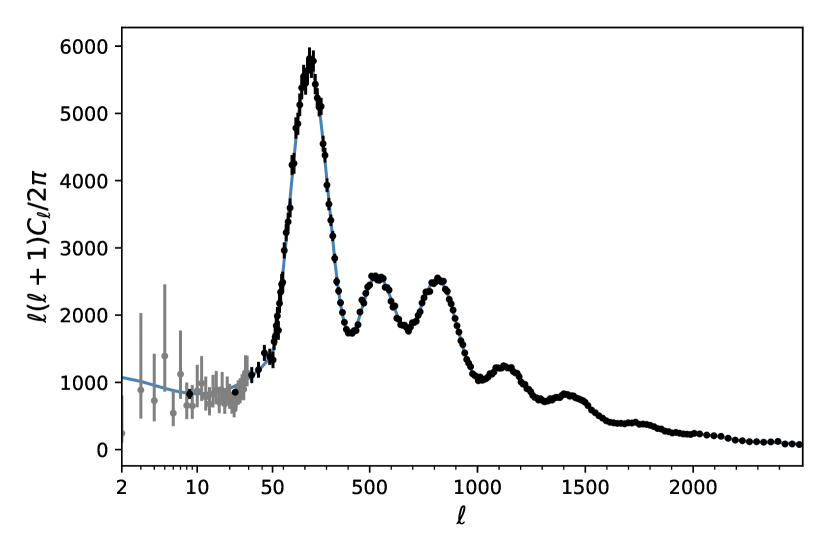
At $\ell\geq 30$ (corresponding to scales smaller than several degrees on the sky) the likelihood $\mathcal{L}$ for the temperature and $E$-mode polarization power spectra (TT, TE, and EE) is modeled as a Gaussian distribution, with

$$-2\ln\mathcal{L}=(C_{b}^{\rm th}-C_{b}^{\rm data})^{T}Q^{-1}(C_{b}^{\rm th}-C_{b}^{\rm data})$$ (1)

to within an overall additive constant, with binned data $C_{b}^{\rm data}$, binned theory $C_{b}^{\rm th}$, and binned covariance matrix $Q$. For the Plik_lite likelihood (Planck Collaboration, 2016a), these data spectra represent an estimate of the CMB bandpowers, with foregrounds already marginalized over using the approach of Dunkley et al. (2013).

At $\ell<30$ the distribution of the angular power spectrum is non-Gaussian. For the 2015 data release, the Planck team released a joint pixel based likelihood for temperature and polarization for $\ell\leq 29$ (‘lowTEB’). There is also a standalone temperature low-$\ell$ likelihood based on the foreground-cleaned Commander temperature map, which we use in this paper. These likelihoods are computed in map space since the distribution of the power spectrum on these scales is non-Gaussian. The 2018 likelihood uses a similar low-$\ell$ temperature likelihood, and a separate low-$\ell$ polarization likelihood built from simulations (Planck Collaboration, 2019).

II.1 Low-$\ell$ temperature bins

The compression approach we adopt, which we describe in the next section, is optimal for Gaussian distributions. Since we are interested in a lightweight compression to estimate simple cosmological models, we first compress the $\ell<30$ Planck TT data into two bins with approximately Gaussian distributions. We do this by conditionally sampling the posterior distribution for the power in each bin, estimating

$$p(\theta|d)\propto p(d|\theta)p(\theta).$$ (2)

Here the parameters $\theta$ are the binned values $D_{2\leq\ell\leq 15}$ and $D_{16\leq\ell\leq 29}$, where $D_{\ell}=\ell(\ell+1)C_{\ell}/2\pi$, assuming a constant value for $D$ in each bin. The likelihood $p(d|\theta)$ is the Planck $\ell<30$ temperature likelihood function. We assume uniform priors on $\theta$. The binning is performed on $D_{\ell}$ rather than $C_{\ell}$ because $D_{\ell}$ is approximately constant for the low-$\ell$ temperature power spectrum. When binned values of $C$ are required we convert from the binned $D$ values by dividing by the mean of $\ell(\ell+1)/2\pi$ in the bin.

Figure 2: The probability distribution for $D_{\ell}$ for two low-$\ell$ temperature bins using the Planck 2015 low-$\ell$ Commander likelihood. The best-fit Gaussian distribution is shown in blue.

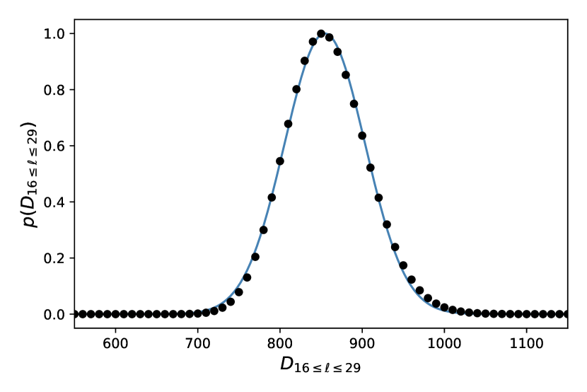
The distributions of the two low-$\ell$ power spectrum bins are shown in Fig. 2, together with the best-fitting Gaussian distributions. We find

$$D_{2\leq\ell\leq 15}=827\pm 74\leavevmode\nobreak\ \mu{\rm K}^{2}$$

$$D_{16\leq\ell\leq 29}=854\pm 49\leavevmode\nobreak\ \mu{\rm K}^{2}.$$ (3)

Their distributions are close to Gaussian, unlike the distributions for the individual multipoles. These bandpowers are also indicated in Fig. 1 (the first two black points), together with the unbinned low-$\ell$ power spectrum in gray. We chose this binning scheme before sampling parameters; other choices that produce approximately Gaussian distributions would be expected to give similar results.

II.2 Low-$\ell$ polarization ($\tau$ prior)

The amplitude of the large-scale polarization signal depends primarily on the optical depth to reionization, as well as the primordial amplitude. To include the low-$\ell$ polarization data we compress the 2015 polarization information into a single Gaussian prior on the optical depth to reionization, adopting $\tau=0.067\pm 0.023$ derived from the Planck low-$\ell$ likelihood using the Low Frequency Instrument (Planck Collaboration, 2016a). This is an approximation since $\tau$ is correlated with other cosmological parameters, in particular the primordial amplitude $A_{s}$. Improved measurements of the optical depth have since been made from the Planck High Frequency Instrument Planck Collaboration (2016c); Planck Collaboration (2018). However, the purpose of this study is to compress the public 2015 likelihood, and we defer a future refinement of our compression code to include the 2018 polarization information that was recently made public.

II.3 Parameter constraints

The effect of describing the low-$\ell$ temperature data using two Gaussian bins and using a prior on $\tau$ in place of the low-$\ell$ polarization likelihood is shown in Fig. 3, which shows the posterior probabilities for the six $\Lambda$CDM parameters (the Hubble constant, baryon density, cold dark matter density, amplitude and spectral index of primordial fluctuations, and optical depth to reionization) obtained by sampling three different likelihood combinations.

Figure 3: Posteriors on the $\Lambda$CDM parameters from Planck-lite-py, a Python implementation of the Planck Plik_lite likelihood with two Gaussian low-$\ell$ bins (black solid curve) compared to the combined Plik_lite TT + low-$\ell$ Commander Planck 2015 temperature likelihoods (blue-dashed curve). The parameter constraints agree to within 0.1$\sigma$, showing that our two binned low-$\ell$ data points capture enough information to give equivalent constraints to the full low-$\ell$ temperature likelihood. A Gaussian prior of $\tau=0.067\pm 0.023$ is included in the black and blue curves. We also show results from the public chains from sampling the TT+lowTEB Planck 2015 likelihood (gray solid curve) for reference. The small difference is the effect of imposing a prior on the optical depth.

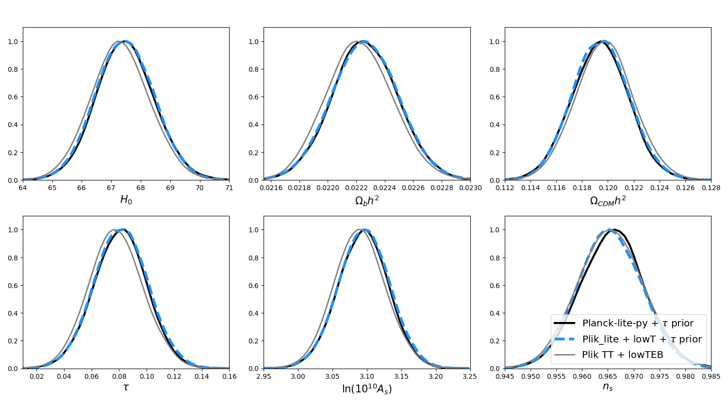
Replacing the low-$\ell$ temperature likelihood with a Gaussian likelihood based on two low-$\ell$ temperature bins results in parameter constraints that agree well, to within 0.1$\sigma$ (black versus blue-dashed in Fig. 3). Here, the black solid curve is derived using our Python implementation of Plik_lite with the additional two Gaussian low-$\ell$ bins included (Planck-lite-py). The blue-dashed curve shows the posteriors obtained by sampling the Planck high-$\ell$ temperature Plik_lite and low-$\ell$ temperature-only Commander likelihoods using the CosmoSIS cosmological parameter estimation code (Zuntz et al., 2015). In both cases we compute the theoretical CMB power spectrum using the Cosmic Linear Anisotropy Solving System (CLASS) (Blas et al., 2011), sample the likelihood using the emcee (Foreman-Mackey et al., 2013) Python implementation of Markov chain Monte Carlo (MCMC) affine-invariant ensemble sampling (Goodman and Weare, 2010), and impose a Gaussian prior on the optical depth $\tau=0.067\pm 0.023$ from the Planck low-$\ell$ likelihood (Planck Collaboration, 2016a). The low-$\ell$ data provide an important anchor for constraints on parameters such as spectral index $n_{s}$ and Hubble parameter $h$. The Planck-lite-py parameter constraints agree with the Plik_lite+lowT constraints to within 0.1$\sigma$, showing that for the standard cosmological model the full low-$\ell$ temperature likelihood can be replaced by a Gaussian likelihood with two bins and a diagonal covariance matrix without a significant effect on the parameter constraints.

The gray curve in Fig. 3 shows the public Planck 2015 chains from the TT+lowTEB likelihood. When comparing parameters constraints from the full TT+lowTEB likelihood with the TT+lowT+$\tau$ prior likelihood some of the parameters shift by up to 0.2$\sigma$ because we are using a tau prior which is only an approximation to the full low-$\ell$ polarization likelihood.

We make available Planck-lite-py, a Python implementation of the Planck Plik_lite likelihood that includes these low-$\ell$ binned temperature data.

III MOPED compression vectors

We use the Massively Optimized Parameter Estimation and Data compression technique (MOPED) described in Heavens et al. (2000) to compress the Planck power spectrum. This linear compression is optimal in the sense that the Fisher information content is preserved for Gaussian data when the covariance matrix is independent of the parameters of interest.

The Planck data vector used in this analysis is the foreground-marginalized binned temperature angular power spectrum. It would be straightforward to include the TE and EE angular power spectra in the data vector for a combined temperature and polarization compressed likelihood. The binning is performed using a constant weighting in $D_{\ell}$ (Planck Collaboration, 2016a), which corresponds to

$$C_{b}=\sum\limits_{\ell=\ell_{b}^{min}}^{\ell_{b}^{max}}w_{b}^{\ell}C_{\ell},$$ (4)

where

$$w_{b}^{\ell}=\frac{\ell(\ell+1)}{\sum\limits_{\ell=\ell_{b}^{min}}^{\ell_{b}^{max}}\ell(\ell+1)}.$$ (5)

The binned angular power spectrum is the sum of a signal component that depends on the cosmological parameters $\boldsymbol{\mu}=C_{b}^{th}$ (the noise-free theoretical binned angular power spectrum), as well as a noise component $\boldsymbol{n}$. The total data vector is thus

$$\boldsymbol{x}=\boldsymbol{\mu}+\boldsymbol{n}.$$ (6)

The data vector can be compressed into a single number while preserving the information about the first cosmological parameter of interest $\theta_{1}$ Tegmark et al. (1997)

$$y_{1}=\boldsymbol{b_{1}}^{t}\boldsymbol{x}$$ (7)

with

$$\boldsymbol{b_{1}}=\frac{\boldsymbol{Q}^{-1}\boldsymbol{\mu}_{,1}}{\sqrt{\boldsymbol{\mu}^{t}_{,1}\boldsymbol{Q}^{-1}\boldsymbol{\mu}^{t}_{,1}}},$$ (8)

where $\boldsymbol{\mu}_{,1}$ is the derivative of the signal (the theoretical binned temperature angular power spectrum) with respect to the first cosmological parameter, $\boldsymbol{Q}$ is the covariance matrix, and the normalization of the compression vector has been chosen such that $\boldsymbol{b}_{1}^{t}\boldsymbol{Q}\boldsymbol{b}_{1}=1$.

Additional compression vectors can be found that produce linear combinations which capture information about the other cosmological parameters, while being orthogonal to the other compression vectors so that each linear combination $y_{m}$ is uncorrelated with the others Heavens et al. (2000), giving

$$\boldsymbol{b}_{m}=\frac{\boldsymbol{Q}^{-1}\boldsymbol{\mu}_{,m}-\sum\limits_{q=1}^{m-1}(\boldsymbol{\mu}_{,m}^{t}\boldsymbol{b}_{q})\boldsymbol{b}_{q}}{\sqrt{\boldsymbol{\mu}_{,m}\boldsymbol{Q}^{-1}\boldsymbol{\mu}_{,m}-\sum\limits_{q=1}^{m-1}(\boldsymbol{\mu}_{,m}^{t}\boldsymbol{b}_{q})^{2}}}.$$ (9)

Figure 4: Compression vectors for the $\Lambda$CDM parameters. The sharp features are caused by binning of the power spectrum. These compression vectors can be applied to the CMB temperature power spectrum to give six numbers that contain as much information about the cosmological parameters as the binned temperature power spectrum. The compression vectors depend on the order in which they are computed, as they are intentionally orthogonal to one another.

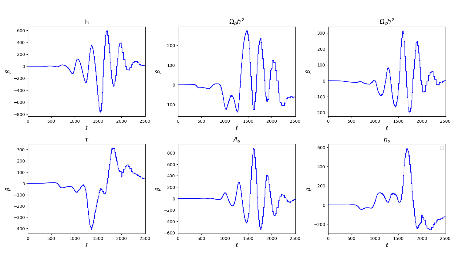
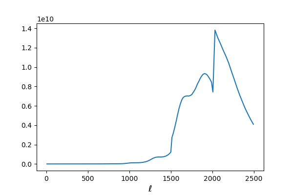
The compression vectors for the six standard $\Lambda$CDM parameters are shown in Fig. 4. The oscillatory behavior comes from the effect of the acoustic peaks on the derivatives of the theoretical CMB power spectrum. Most of the signal comes from $1000<\ell<2500$ because this is where the diagonal of the binned inverse covariance matrix is large (Fig. 5). At low $\ell$ cosmic variance dominates the noise while at high $\ell$ experimental noise takes over. The noise in each bin is also dependent on the bin width, which varies for different multipoles (Planck Collaboration, 2016a).

Figure 5: The diagonal of the binned temperature inverse covariance matrix for the 217 temperature bins (2 for low-$\ell$ and 215 for high-$\ell$). The diagonal elements are small for $\ell<1000$, then rise steeply for $1500<\ell<2000$ before dropping again when the experimental noise approaches the signal.

Applying these compression vectors to the data vector

$$y_{m}=\boldsymbol{b_{m}}^{t}\boldsymbol{x}$$ (10)

gives a set of $M$ numbers $y_{m},m=1,...,M$ which contain as much information about the cosmological parameters of interest $\theta_{m}$ as the full angular power spectrum with $N$ bins. For the binned temperature power spectrum the data vector has length $N=217$, and for the standard $\Lambda$CDM cosmology the number of parameters of interest is $M=6$.

The Planck power spectrum and covariance matrix that are used to compute the compression vectors are already binned, so the compressed statistics for the data come from applying binned compression vectors to the power spectrum. To compress the theoretical CMB power spectrum we use a version of the compression vectors that includes the binning, weighting each multipole appropriately as per Eq. (4), so that the binning and compression are achieved in the same step.

Figure 6: Posteriors on the $\Lambda$CDM parameters from the compressed CosMOPED likelihood (red-dashed curves) and the Planck-lite-py Python implementation of the Plik_lite likelihood with two low-$\ell$ bins (black solid curves). The parameter constraints agree to within 0.1$\sigma$, validating the CosMOPED compression scheme. A Gaussian prior of $\tau=0.067\pm 0.023$ is included for both curves.

IV Likelihood and parameters

We now describe the compressed likelihood and compare it to our Planck-lite-py implementation of the Planck 2015 Plik_lite likelihood.

IV.1 Format of the likelihood

Each compressed statistic $y_{m}$ is Gaussian distributed with unit variance. The $y_{m}$’s are uncorrelated with each other by design, so the total likelihood is the product of the likelihoods from each statistic. The likelihood of the parameters given the (compressed) data thus takes a simple form

$$-2\ln\mathcal{L}=\sum_{m=1}^{M}\frac{(y_{m}-\langle y_{m}\rangle)^{2}}{2}+\text{constant},$$ (11)

where $y_{m}$ is the compressed statistic from the data and $\langle y_{m}\rangle=\boldsymbol{b_{m}}^{t}\boldsymbol{\mu}$ is the corresponding compressed statistic from the model (the theoretical temperature power spectrum).

IV.2 Parameter constraints

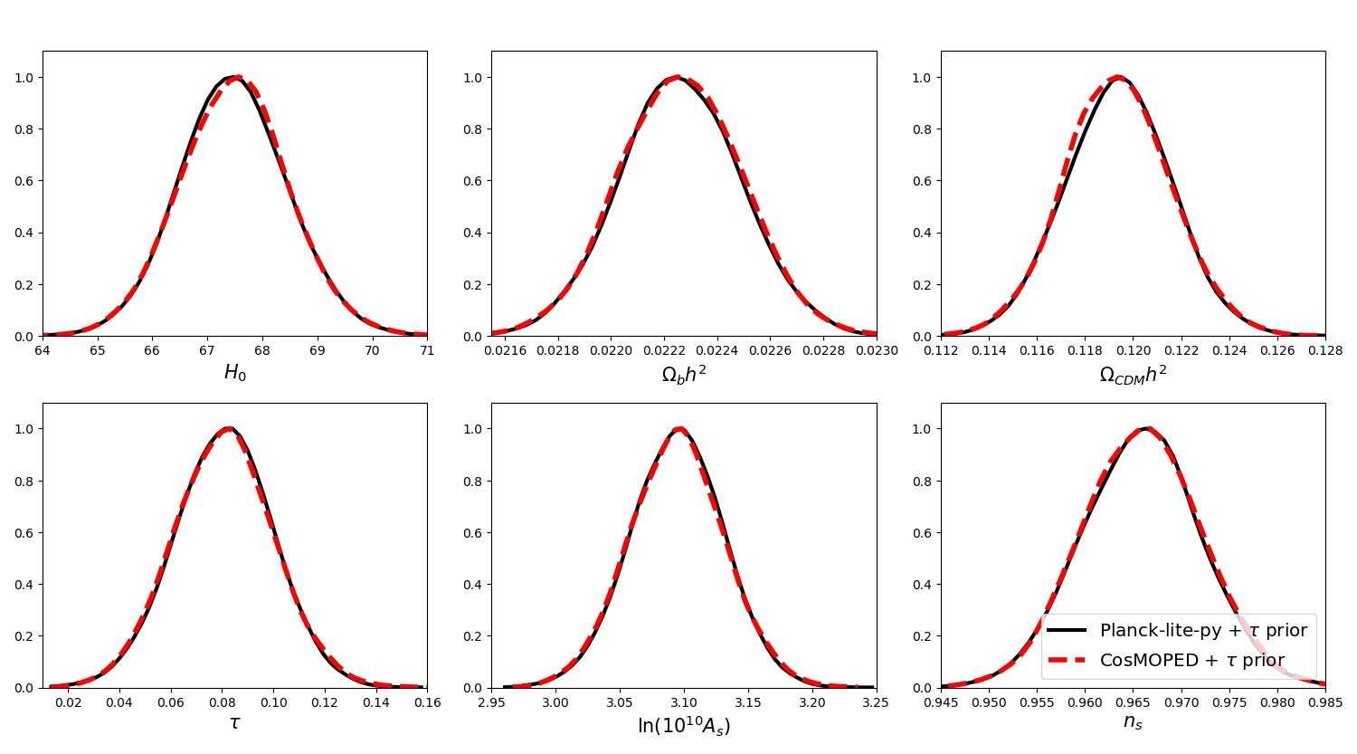
The parameter constraints for the six-parameter $\Lambda$CDM model are shown in Fig. 6. The compressed likelihood (red-dashed curve) and the Python Plik_lite implementation (black solid curve) agree to within $0.1\sigma$ for each parameter. Both likelihoods were sampled with emcee, with a Gaussian prior on the optical depth $\tau=0.067\pm 0.023$ and the low-$\ell$ bins described in Sec. II. The MOPED compression that we have applied thus results in a likelihood that is equivalent to the uncompressed case. As we showed earlier, the Python Plik_lite implementation is in good agreement with the full Planck temperature likelihood.

IV.3 Effect of fiducial model

The theory vector $\boldsymbol{\mu}$ used to compute the compression vectors depends on the fiducial model parameters used. If the fiducial model is wrong then the compression is no longer optimal and the $M$ compressed statistics are not exactly independent. However, in practice using a different fiducial model does not have a significant effect on the compressed likelihood, in agreement with the findings of Zablocki and Dodelson (2016). A shift of order 3$\sigma$ in the fiducial parameters has an insignificant effect on the conditional probability slices obtained from the compressed likelihood.

Figure 7: The constraints on running of the scalar spectral index from the compressed CosMOPED likelihood (red dashed) agree to within 0.1$\sigma$ with the uncompressed Planck-lite-py (black). A Gaussian prior of $\tau=0.067\pm 0.023$ is used for CosMOPED and Planck-lite-py. The distribution using the public Planck chains (TT+lowTEB, gray) is slightly broader due to the more accurate treatment of low-$\ell$ polarization.

IV.4 Non-$\Lambda$CDM cases

We demonstrate the application of this compression technique to a one parameter extension to the $\Lambda$CDM case by sampling running of the scalar spectral index $d\ln n_{s}/d\ln k$ in addition to the six $\Lambda$CDM parameters shown above.

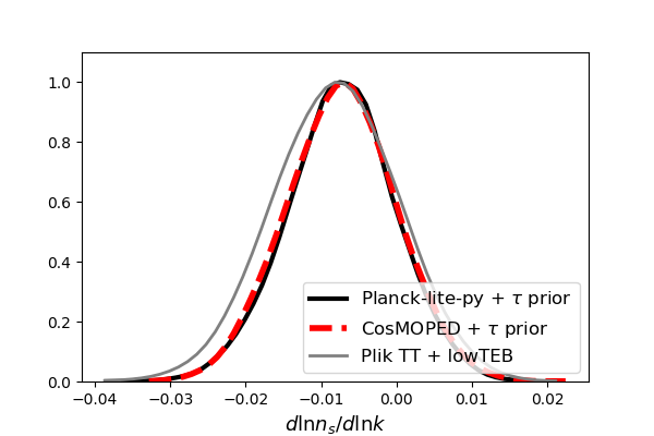
The results are shown in Fig. 7, which compares the CosMOPED constraints to the Planck-lite-py constraints (with the same $\tau$ prior as above), as well as the Planck TT+lowTEB chains from the 2015 data release. The likelihoods show excellent agreement. The CosMOPED and Planck-lite-py posteriors are slightly narrower than for the Planck TT+lowTEB chains; this is because the Gaussian prior on $\tau$ which we use in the CosMOPED likelihood comes from the low-$\ell$ likelihood assuming the $\Lambda$CDM model. For $\Lambda$CDM extension models with parameters that correlate with $\tau$, this prior is slightly too narrow.

V Discussion and conclusion

We have demonstrated that the low-$\ell$ Planck temperature data is well represented by two Gaussian bins for simple cosmological models. We have also shown that applying MOPED linear compression to the Planck 2015 binned temperature power spectrum allows us to construct a simple likelihood that depends on just one compression vector and one compressed statistic per parameter of interest, and which is equivalent to the Plik-lite temperature likelihood with two low-$\ell$ bins included. Because we do not directly incorporate the low-$\ell$ polarization likelihood, we recommend including a prior on the optical depth to reionization $\tau$ when using either of these likelihoods.

We provide two public codes. The first is Planck-lite-py, an implementation of Planck’s Plik_lite likelihood in Python, with the option to include the low-$\ell$ temperature data as two Gaussian bins. The second is CosMOPED, which calculates the MOPED compression vectors for the CMB temperature power spectrum and computes the compressed Planck likelihood.

This method can easily be extended to incorporate the high-$\ell$ TE and EE data which are also Gaussian distributed. It can also be used for the Planck 2018 likelihood, and the publicly available code will be updated accordingly.

The MOPED data compression scheme provides a lightweight likelihood that can easily be combined with other datasets. In addition, the compressed data can be incorporated into a likelihood free inference framework which allows parameters to be inferred based on forward simulations, without knowledge of the form of the likelihood. In likelihood free inference it is useful to have informative compressed statistics, because this makes the comparison of simulations and data much less computationally intensive.

VI Acknowledgments

We thank Erminia Calabrese for useful comments. We acknowledge the use of data and code from the Planck Legacy Archive.

References

- Tegmark et al. (1997) M. Tegmark, A. N. Taylor, and A. F. Heavens, Karhunen-Loève Eigenvalue Problems in Cosmology: How Should We Tackle Large Data Sets?, Astrophys. J. 480, 22 (1997), astro-ph/9603021 .
- Heavens et al. (2000) A. F. Heavens, R. Jimenez, and O. Lahav, Massive lossless data compression and multiple parameter estimation from galaxy spectra, Monthly Notices of the Royal Astronomical Society 317, 965 (2000), astro-ph/9911102 .
- Alsing and Wandelt (2018) J. Alsing and B. Wandelt, Generalized massive optimal data compression, Monthly Notices of the Royal Astronomical Society 476, L60 (2018), arXiv:1712.00012 [astro-ph.CO] .
- Reichardt et al. (2001) C. Reichardt, R. Jimenez, and A. F. Heavens, Recovering physical parameters from galaxy spectra using MOPED, Monthly Notices of the Royal Astronomical Society 327, 849 (2001), arXiv:astro-ph/0101074 [astro-ph] .
- Heavens et al. (2004) A. Heavens, B. Panter, R. Jimenez, and J. Dunlop, The star-formation history of the Universe from the stellar populations of nearby galaxies, Nature (London) 428, 625 (2004), arXiv:astro-ph/0403293 [astro-ph] .
- Panter et al. (2007) B. Panter, R. Jimenez, A. F. Heavens, and S. Charlot, The star formation histories of galaxies in the Sloan Digital Sky Survey, Monthly Notices of the Royal Astronomical Society 378, 1550 (2007), arXiv:astro-ph/0608531 [astro-ph] .
- Protopapas et al. (2005) P. Protopapas, R. Jimenez, and C. Alcock, Fast identification of transits from light-curves, Monthly Notices of the Royal Astronomical Society 362, 460 (2005), arXiv:astro-ph/0502301 [astro-ph] .
- Graff et al. (2011) P. Graff, M. P. Hobson, and A. Lasenby, An investigation into the Multiple Optimised Parameter Estimation and Data compression algorithm, Monthly Notices of the Royal Astronomical Society 413, L66 (2011), arXiv:1010.5907 [astro-ph.IM] .
- Heavens et al. (2017) A. F. Heavens, E. Sellentin, D. de Mijolla, and A. Vianello, Massive data compression for parameter-dependent covariance matrices, Monthly Notices of the Royal Astronomical Society 472, 4244 (2017), arXiv:1707.06529 [astro-ph.CO] .
- Gupta and Heavens (2002) S. Gupta and A. F. Heavens, Fast parameter estimation from the cosmic microwave background power spectrum, Monthly Notices of the Royal Astronomical Society 334, 167 (2002), arXiv:astro-ph/0108315 [astro-ph] .
- Zablocki and Dodelson (2016) A. Zablocki and S. Dodelson, Extreme data compression for the CMB, Phys. Rev. D 93, 083525 (2016), arXiv:1512.00072 [astro-ph.CO] .
- Planck Collaboration (2018) Planck Collaboration, Planck 2018 results. VI. Cosmological parameters, arXiv e-prints , arXiv:1807.06209 (2018), arXiv:1807.06209 [astro-ph.CO] .
- Planck Collaboration (2016a) Planck Collaboration, Planck 2015 results. XI. CMB power spectra, likelihoods, and robustness of parameters, Astronomy and Astrophysics 594, A11 (2016a), arXiv:1507.02704 [astro-ph.CO] .
- Planck Collaboration (2016b) Planck Collaboration, Planck 2015 results. XIII. Cosmological parameters, Astronomy and Astrophysics 594, A13 (2016b), arXiv:1502.01589 [astro-ph.CO] .
- Blas et al. (2011) D. Blas, J. Lesgourgues, and T. Tram, The Cosmic Linear Anisotropy Solving System (CLASS). Part II: Approximation schemes, Journal of Cosmology and Astroparticle Physics 2011, 034 (2011), arXiv:1104.2933 [astro-ph.CO] .
- Dunkley et al. (2013) J. Dunkley, E. Calabrese, J. Sievers, et al., The Atacama Cosmology Telescope: likelihood for small-scale CMB data, Journal of Cosmology and Astroparticle Physics 2013, 025 (2013), arXiv:1301.0776 [astro-ph.CO] .
- Planck Collaboration (2019) Planck Collaboration, Planck 2018 results. V. CMB power spectra and likelihoods, arXiv e-prints , arXiv:1907.12875 (2019), arXiv:1907.12875 [astro-ph.CO] .
- Planck Collaboration (2016c) Planck Collaboration, Planck intermediate results. XLVII. Planck constraints on reionization history, Astronomy and Astrophysics 596, A108 (2016c), arXiv:1605.03507 .
- Zuntz et al. (2015) J. Zuntz, M. Paterno, E. Jennings, D. Rudd, A. Manzotti, S. Dodelson, S. Bridle, S. Sehrish, and J. Kowalkowski, CosmoSIS: Modular cosmological parameter estimation, Astronomy and Computing 12, 45 (2015), arXiv:1409.3409 [astro-ph.CO] .
- Foreman-Mackey et al. (2013) D. Foreman-Mackey, D. W. Hogg, D. Lang, and J. Goodman, emcee: The MCMC Hammer, Publications of the Astronomical Society of the Pacific 125, 306 (2013), arXiv:1202.3665 [astro-ph.IM] .
- Goodman and Weare (2010) J. Goodman and J. Weare, Ensemble samplers with affine invariance, Communications in Applied Mathematics and Computational Science 5, 65 (2010).