Explicit-Duration Markov Switching Models

Abstract

Markov switching models (MSMs) are probabilistic models that employ multiple sets of parameters to describe different dynamic regimes that a time series may exhibit at different periods of time. The switching mechanism between regimes is controlled by unobserved random variables that form a first-order Markov chain. Explicit-duration MSMs contain additional variables that explicitly model the distribution of time spent in each regime. This allows to define duration distributions of any form, but also to impose complex dependence between the observations and to reset the dynamics to initial conditions. Models that focus on the first two properties are most commonly known as hidden semi-Markov models or segment models, whilst models that focus on the third property are most commonly known as changepoint models or reset models. In this monograph, we provide a description of explicit-duration modelling by categorizing the different approaches into three groups, which differ in encoding in the explicit-duration variables different information about regime change/reset boundaries. The approaches are described using the formalism of graphical models, which allows to graphically represent and assess statistical dependence and therefore to easily describe the structure of complex models and derive inference routines. The presentation is intended to be pedagogical, focusing on providing a characterization of the three groups in terms of model structure constraints and inference properties. The monograph is supplemented with a software package that contains most of the models and examples described. The material presented should be useful to both researchers wishing to learn about these models and researchers wishing to develop them further.

Chapter 1 Introduction

Markov switching models (MSMs) are probabilistic models that employ multiple sets of parameters to describe different dynamic regimes that a time series may exhibit at different periods of time. The switching mechanism between regimes is controlled by unobserved variables that form a first-order Markov chain.

MSMs are commonly used for segmenting time series or to retrieve the hidden dynamics underlying noisy observations.

Consider, for example, the time series displayed in Figure 1.1(a), which corresponds to the measured leg positions of an individual performing repetitions of the actions low/high jumping and hopping on the left/right foot. A segmentation of the time series into the underlying actions could be obtained with a MSM in which each action forms a separate regime, e.g. by computing the regimes with highest posterior probabilities.

As another example, consider the time series displayed with dots in Figure 1.1(b), which corresponds to noisy observations of the positions of a two-wheeled robot moving in the two-dimensional space according to straight movements, left-wheel rotations and right-wheel rotations (the actual positions are displayed with a continuous line). Denoised estimates of the positions could be obtained with a MSM in which the robot movements are described with continuous unobserved variables and in which each type of movement forms a separate regime, e.g. by computing the posterior means of the continuous variables.

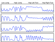
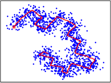
Figure 1.1: (a): Body-marker recording of an individual performing repetitions of the actions low jumping up and down, high jumping up and down, hopping on the left foot and hopping on the right foot (CMU Graphics Lab Motion Capture Database). (b): Actual positions (continuous line) and measured positions (dots) of a two-wheeled robot moving in the two-dimensional space. The initial actual position is indicated with a star.

In standard MSMs, the regime variables implicitly define a geometric distribution on the time spent in each regime. In explicit-duration MSMs, this constraint is relaxed by using additional unobserved variables that allow to define duration distributions of any form. Explicit-duration variables also allow to impose complex dependence between the observations and to reset the dynamics to initial conditions.

Explicit-duration MSMs were first introduced in the speech community (Ferguson, 1980) and are mostly used to achieve more powerful modelling than standard MSMs through the specification of more accurate duration distributions and dependencies between the observations. In this case, the models are most commonly known with the names of hidden semi-Markov models or segment models. However, the possibility to reset the dynamics to initial conditions has recently led to the use of explicit-duration variables also for Bayesian approaches to abrupt-change detection, for identifying repetitions of patterns (such as, e.g., the action repetitions underlying the time series in Figure 1.1(a)), and for performing/approximating inference (Fearnhead, 2006; Fearnhead and Vasileiou, 2009; Chiappa and Peters, 2010; Bracegirdle and Barber, 2011). In these cases, the models are most commonly known with the names of changepoint models or reset models.

Explicit-duration MSMs have been used in many application areas including speech analysis (Russell and Moore, 1985; Levinson, 1986; Rabiner, 1989; Gu et al., 1991; Gales and Young, 1993; Russell, 1993; Ostendorf et al., 1996; Moore and Savic, 2004; Liang et al., 2011), handwriting recognition (Chen et al., 1995), activity recognition (Yu and Kobayashi, 2003b; Huang et al., 2006; Oh et al., 2008; Chiappa and Peters, 2010), musical pattern recognition (Pikrakis et al., 2006), financial time series analysis (Bulla and Bulla, 2006), rainfall time series analysis (Sansom and Thomson, 2001), protein structure segmentation (Schmidler et al., 2000), gene finding (Winters-Hilt et al., 2010), DNA analysis (Barbu and Limnios, 2008; Fearnhead and Vasileiou, 2009), plant analysis (Guédon et al., 2001), MRI sequence analysis (Faisan et al., 2002), ECG segmentation (Hughes et al., 2004), and waveform modelling (Kim and Smyth, 2006); see references in Yu (2010) for more examples.

Explicit-duration MSMs originated from the idea of explicitly modelling the duration distribution by defining a semi-Markov process on the regime variables, namely a process in which the trajectories are piecewise constant functions – with interval durations drawn from an explicitly defined duration distribution – and in which the variables at jump times form a Markov chain. The first and currently standard approach achieves that with variables indicating the interval duration, and derives inference recursions using only jump times (Rabiner, 1989; Gales and Young, 1993; Ostendorf et al., 1996; Yu, 2010). To simplify the derivations of posterior distributions at times that are different from jump times, Chiappa and Peters (2010) use count variables in addition to duration variables, such that the combined regime and count-duration variables form a first-order Markov chain. Other methods that explicitly model the duration distribution have been proposed with different goals and in different communities. These methods can all be viewed as different ways to define a first-order Markov chain on the combined regime and explicit-duration variables that induces a semi-Markov process on the regime variables.

In this monograph we provide a description of explicit-duration modelling that aims at elucidating the characteristics of the different approaches and at clarifying and unifying the literature. We identify three fundamentally different ways to define the first-order Markov chain on the combined regime and explicit-duration variables, which differ in encoding in the explicit-duration variables the location of (i) the preceding, (ii) the following, or (iii) both the preceding and following regime change or reset. We discuss each encoding in the context of MSMs of simple unobserved structure and of MSMs that contain extra unobserved variables related by first-order Markovian dependence. The models are described using the formalism of graphical models, which allows to graphically represent and assess statistical dependence, and therefore to easily describe the structure of complex models and derive inference routines.

The remainder of the manuscript is organized as follows. Chapter 2 contains some background material. We start with a general description of MSMs and by showing that the regime variables implicitly define a geometric duration distribution. In §2.1 we introduce the hidden Markov model, which represents the simplest MSM, and explain how to obtain a negative binomial duration distribution with regime copies. In §2.2 we introduce the framework of graphical models, and explain how to graphically assess statistical independence in a particular type of graphical models, called belief networks, that will be used for describing the models. In §2.2.1 we illustrate how belief networks can be used to easily derive the standard inference recursions of MSMs. In §2.3 we give a general explanation of the expectation maximization algorithm, which represents the most popular algorithm for parameter learning in probabilistic models with unobserved variables. In Chapter 3 we describe the different approaches to explicit-duration modelling by categorizing them into three groups. The groups are introduced in §3.1, §3.2 and §3.3. In §3.4 we discuss in detail explicit-duration modelling in MSMs containing only regime variables, explicit-duration variables, and observations. In §3.5 we discuss in detail explicit-duration modelling in a popular MSM containing additional unobserved variables related by first-order Markovian dependence, namely the switching linear Gaussian state-space model, and discuss how the findings generalize to similar models with unobserved variables related by first-order Markovian dependence. The case of more complex unobserved structure is not considered. In §3.6 we describe approximation schemes to reduce the computational cost of inference. In Chapter 4 we summarize the most important points of our exposition and make some historical remarks.

Chapter 2 Background

Markov switching models (MSMs) describe a time series $v_{1},\ldots,v_{T}=v_{1:T}$ using $S$ different sets of parameters, each defining a different dynamic regime. This is achieved by using unobserved variables $s_{1:T}$, where $s_{t}\in\{1,\ldots,S\}$ indicates which of the $S$ regimes underlies observations $v_{t}$. The regime variables form a first-order, time-homogeneous, Markov chain, i.e. the joint distribution $p(s_{1:T})$ can be written as

$$p(s_{1:T})=p(s_{1})\prod_{t=2}^{T}p(s_{t}|s_{t-1})=\tilde{\pi}_{s_{1}}\prod_{t=2}^{T}\pi_{s_{t}s_{t-1}},$$

where $\tilde{\pi}$ is a vector of elements $\tilde{\pi}_{s_{1}}=p(s_{1})$ and $\pi$ is a time-independent transition matrix of elements $\pi_{s_{t}s_{t-1}}=p(s_{t}|s_{t-1})$.

In standard MSMs, the regime variables implicitly define a geometric distribution on the time spent in each regime. Indeed, given e.g. $s_{t}=i$, the probability of remaining in regime $i$ at time-steps $t+1,\ldots,t+d-1$ and switching to a different regime at time-step $t+d$ is

$$p(s_{t+1:t+d-1}\!=\!i,s_{t+d}\!\neq\!i|s_{t}\!=\!i) =\pi_{ii}^{d-1}\sum_{j\neq i}\pi_{ji}=\pi_{ii}^{d-1}(1\!-\!\pi_{ii}),$$

which corresponds to the geometric distribution with parameter $\pi_{ii}$. The geometric distribution with $\pi_{ii}\in\{0.1,0.5,0.9\}$ is shown in Figure 2.1(a).

The remainder of the chapter is organized as follows. In §2.1 we describe the simplest MSM, namely the hidden Markov model, and show that a negative binomial duration distribution can be obtained with regime copies. In §2.2 we introduce the formalism of graphical models and show how this formalism can be used to derive the standard inference recursions of MSMs – a similar approach will be employed to derive inference recursions in the explicit-duration extensions. In §2.3 we describe the expectation maximization algorithm, which will be used for parameter learning throughout the manuscript.

2.1 Hidden Markov Model

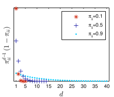
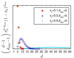
Figure 2.1: (a): Geometric duration distribution implicitly defined in a standard MSM with $\pi_{ii}\in\{0.1,0.5,0.9\}$. (b): Negative binomial duration distribution obtained by replacing regime $i$ in the standard MSM in (a) with $d_{\min}=5$ copies.

The hidden Markov model (HMM) (Rabiner, 1989) is defined by a joint distribution $p(s_{1:T},v_{1:T})$ that factorizes as

$$p(s_{1:T},v_{1:T})=p(v_{1}|s_{1})p(s_{1})\prod_{t=2}^{T}p(v_{t}|s_{t})p(s_{t}|s_{t-1}),$$ (2.1)

where the emission distribution $p(v_{t}|s_{t})$ is time-homogeneous and, for continuous $v_{t}$, commonly modelled as a Gaussian mixture. As discussed above, $s_{1:T}$ implicitly define a geometric duration distribution. A more flexible negative binomial duration distribution can be obtained by imposing a minimum duration $d_{\min}$ on the time spent in a regime (Durbin et al., 1998). This can be achieved, e.g., by replacing the original regimes with $S$ ordered sets of regimes $R_{i}=\{(i-1)d_{\min}+1,\ldots,id_{\min}\}$, $i=1,\ldots,S$, where the elements of $R_{i}$ have the same emission distribution as original regime $i$ and transition distribution

$$p(s_{t+1}|s_{t}\!\in\!R_{i}\!\setminus\!id_{\min})=\begin{cases}\pi_{ii}&\hskip-4.26773pt\textrm{if }s_{t+1}\!=\!s_{t}\\ 1\!-\!\pi_{ii}&\hskip-4.26773pt\textrm{if }s_{t+1}\!=\!s_{t}\!+\!1,\end{cases}$$

$$p(s_{t+1}|s_{t}\!=\!id_{\min})=\begin{cases}\pi_{ii}&\hskip-4.26773pt\textrm{if }s_{t+1}\!=\!s_{t}\\ \pi_{ji}&\hskip-4.26773pt\textrm{if }s_{t+1}\!=\!(j-1)d_{\min}+1,\hskip 2.84544ptj\!\neq\!i.\end{cases}$$

Given $s_{t}=i$, any sequence $s_{t+1},\ldots,s_{t+d-1}$ in $R_{i}$ such that $s_{t+d}\notin R_{i}$ has probability $\pi^{d-1-(d_{\min}-1)}_{ii}(1-\pi_{ii})^{d_{\min}-1}(1-\pi_{ii})$, and there are ${d-1\choose d_{\min}-1}$ such sequences. Therefore

$$p(s_{t+1:t+d-1}\!\in\!R_{i},s_{t+d}\!\notin\!R_{i}|s_{t}\!=\!i)={d\!-\!1\choose d_{\min}\!-\!1}\pi^{d-d_{\min}}_{ii}(1\!-\!\pi_{ii})^{d_{\min}},$$

which corresponds to the negative binomial distribution with parameters $\pi_{ii}$ and $d_{\min}$. The negative binomial distribution with $\pi_{ii}\in\{0.1,0.5,0.9\}$ and $d_{\min}=5$ is shown in Figure 2.1(b).

2.2 Graphical Models and Belief Networks

Figure 2.2: (a): Directed acyclic graph. The node $x_{3}$ is a collider on the path $x_{2},x_{3},x_{1}$ and a non-collider on the path $x_{2},x_{3},x_{4}$. (b): Cyclic graph obtained from (a) by adding a link from $x_{4}$ to $x_{1}$. (c): Belief network representation of the HMM. Rectangular nodes indicate discrete variables, whilst oval nodes indicate discrete or continuous variables. Filled nodes indicate observed variables. This convention is used throughout the manuscript.

Graphical models (Pearl, 1988; Bishop, 2006; Koller and Friedman, 2009; Barber, 2012; Murphy, 2012) are a marriage between graph and probability theory that allows to graphically represent and assess statistical dependence, and therefore to easily describe the structure of complex models and derive inference routines. MSMs are most commonly described using a type of graphical models called belief networks. In the following sections, we give some basic definitions and explain two equivalent methods for graphically assessing statistical independence in belief networks.

Basic definitions

A graph is a collection of nodes and links connecting pairs of nodes. The links may be directed or undirected, giving rise to directed or undirected graphs respectively.
A path from node $x_{i}$ to node $x_{j}$ is a sequence of linked nodes starting at $x_{i}$ and ending at $x_{j}$. A directed path is a path whose links are directed and pointing from preceding towards following nodes in the sequence.
A directed acyclic graph is a directed graph with no directed paths starting and ending at the same node. For example, the directed graph in Figure 2.2(a) is acyclic. The addition of a link from $x_{4}$ to $x_{1}$ gives rise to a cyclic graph (Figure 2.2(b)).
A node $x_{i}$ with a directed link to $x_{j}$ is called parent of $x_{j}$. In this case, $x_{j}$ is called child of $x_{i}$.
A node is a collider on a specified path if it has two parents on that path. Notice that a node can be a collider on a path and a non-collider on another path. For example, in Figure 2.2(a) $x_{3}$ is a collider on the path $x_{2},x_{3},x_{1}$ and a non-collider on the path $x_{2},x_{3},x_{4}$.
A node $x_{i}$ is an ancestor of a node $x_{j}$ if there exists a directed path from $x_{i}$ to $x_{j}$. In this case, $x_{j}$ is a descendant of $x_{i}$.
A graphical model is a graph in which nodes represent random variables and links express statistical relationships between the variables.
A belief network is a directed acyclic graphical model in which each node $x_{i}$ is associated with the conditional distribution $p(x_{i}|\text{par}(x_{i}))$, where $\text{par}(x_{i})$ indicates the parents of $x_{i}$. The joint distribution of all nodes in the graph, $p(x_{1:D})$, is given by the product of all conditional distributions, i.e.

$$p(x_{1:D})=\prod_{i=1}^{D}p(x_{i}|\text{par}(x_{i})).$$

The belief network corresponding to Equation (2.1), and therefore representing the HMM, is given in Figure 2.2(c).

Assessing statistical independence in belief networks

Method I. Given the sets of random variables ${\cal X},{\cal Y}$ and ${\cal Z}$, ${\cal X}$ and ${\cal Y}$ are statistically independent given ${\cal Z}$ (${\cal X}\perp\!\!\!\perp{\cal Y}\,|\,{\cal Z}$) if all paths from any element of ${\cal X}$ to any element of ${\cal Y}$ are blocked. A path is blocked if at least one of the following conditions is satisfied:

1. There is a non-collider on the path which belongs to the conditioning set ${\cal Z}$.

2. There is a collider on the path such that neither the collider nor any of its descendants belong to the conditioning set ${\cal Z}$.

Method II. This method converts the directed graph into an undirected one and then uses the rule of independence for undirected graphs. This is achieved with the following steps:

1. Create the ancestral graph: Remove all nodes that are not in ${\cal X}\cup{\cal Y}\cup{\cal Z}$ and are not ancestors of a node in this set, together with all links in or out of such nodes.

2. Moralize: Add a link between any two nodes that have a common child. Remove arrowheads.

3. Use the independence rule for undirected graphs: ${\cal X}\perp\!\!\!\perp{\cal Y}\,|\,{\cal Z}$ if all paths connecting a node in ${\cal X}$ with one in ${\cal Y}$ pass through a member of ${\cal Z}$.

In Figure 2.3(b) we display the undirected graph obtained from the belief network shown in Figure 2.3(a) after performing steps (IIa) and (IIb) with ${\cal X}=v_{t},{\cal Y}=v_{1:t-2}$ and ${\cal Z}=\{s_{t},v_{t-1}\}$.

Figure 2.3: (a): Belief network representing the extension of the HMM in which the observations are related by first-order Markovian dependence, as indicated by the link from $v_{t-1}$ to $v_{t}$. (b): Undirected graph obtained from the belief network in (a) after performing steps (IIa) and (IIb) with ${\cal X}=v_{t},{\cal Y}=v_{1:t-2}$ and ${\cal Z}=\{s_{t},v_{t-1}\}$.

2.2.1 Inference in MSMs

In this section we illustrate how the formalism of graphical models can be used to derive the standard inference recursions of MSMs.

We consider the extension of the HMM in which the observations (given the regime variables) are related by $k$th-order Markovian dependence, i.e. the joint distribution factorizes as

$$p(s_{1:T},v_{1:T})=\prod_{t=1}^{T}p(v_{t}|s_{t},v_{t-k:t-1})p(s_{t}|s_{t-1}).$$

The introduction of Markovian dependence corresponds to adding links from past to current observations to the belief network representing the HMM, as shown in Figure 2.3(a) for the case of first-order dependence. The most popular model within this class is the switching autoregressive model (Hamilton, 1989, 1990, 1993), also called autoregressive HMM, defined as

$$p(v_{t}|s_{t},v_{t-k:t-1})={\cal N}\Big{(}v_{t};\sum_{i=1}^{k}a^{s_{t}}_{i}v_{t-i},(\sigma^{s_{t}})^{2}\Big{)},$$ (2.2)

where ${\cal N}(x;\mu,\sigma^{2})$ denotes a Gaussian distribution on variable $x$ with mean $\mu$ and variance $\sigma^{2}$, and $a^{s_{t}}_{i}$ is called autoregressive coefficient.

As discussed in Chapter 1, these types of models are often used for time series segmentation. A segmentation can be obtained by computing $s^{*}_{t}=\operatorname*{arg\,max}_{s_{t}}\alpha^{s_{t}}_{t}$ where $\alpha^{s_{t}}_{t}=p(s_{t}|v_{1:t})$ is called the filtered distribution, $s^{*}_{t}=\operatorname*{arg\,max}_{s_{t}}\gamma^{s_{t}}_{t}$ where $\gamma^{s_{t}}_{t}=p(s_{t}|v_{1:T})$ is called the smoothed distribution, or the most likely sequence of regimes $s^{*}_{1:T}=\operatorname*{arg\,max}_{s_{1:T}}p(s_{1:T}|v_{1:T})$. Unknown model parameters can be learned with similar quantities. These quantities can be efficiently computed using time-recursive routines, namely routines which at each time-step make use of computations previously performed at the preceding or following time-step (e.g. $\alpha^{s_{t}}_{t}$ can be computed from $\alpha^{s_{t-1}}_{t-1}$ and $\gamma^{s_{t}}_{t}$ can be computed from $\gamma^{s_{t+1}}_{t+1}$).

In the following sections we describe the two most common approaches to compute the filtered and smoothed distributions, namely parallel and sequential filtering-smoothing, and an extension of Viterbi decoding for computing the most likely sequence of regimes.

The approaches described can be applied to all models in which the unobserved variables form a first-order Markov chain – including the case in which these variables are continuous, by replacing sums with integrations – although computational tractability is not guaranteed. As the explicit-duration MSMs described in Chapter 3 are extensions of the standard MSMs in which the combined regime and explicit-duration variables, $\sigma_{1:T}$, form a first-order Markov chain, we will be able to use similar approaches to derive inference recursions for $\sigma_{1:T}$, which will then be simplified using the deterministic constraints of the Markov chain. Furthermore, as the continuous unobserved variables of the explicit-duration linear Gaussian state-space model described in §3.5 are related by first-order Markovian dependence, we will also be able to use similar approaches to derive inference recursions on these variables. In the case considered in §3.4.3, in which the time series is formed by segments whose observations are related by non-Markovian dependence, time-steps at the segment boundaries only will need to be considered, giving rise to segment-recursive routines.

Parallel filtering-smoothing

The filtered distribution $\alpha^{s_{t}}_{t}=p(s_{t}|v_{1:t})$ can be obtained by normalizing $\bar{\alpha}^{s_{t}}_{t}=p(s_{t},v_{1:t})$, where $\bar{\alpha}^{s_{t}}_{t}$ can be recursively computed as

$$\bar{\alpha}^{s_{t}}_{t} =p(v_{t}|s_{t},\cancel{v_{1:t-k-1}},v_{t-k:t-1})\sum_{s_{t-1}}p(s_{t}|s_{t-1},\cancel{v_{1:t-1}})p(s_{t-1},v_{1:t-1})$$

$$=p(v_{t}|s_{t},v_{t-k:t-1})\sum_{s_{t-1}}\pi_{s_{t}s_{t-1}}\bar{\alpha}^{s_{t-1}}_{t-1}.$$ (2.3)

The independence relation $v_{t}\perp\!\!\!\perp v_{1:t-k-1}\,|\,\{s_{t},v_{t-k:t-1}\}$ can be graphically assessed by observing that (considering, for simplicity, $k=1$) all paths from $v_{1:t-2}$ to $v_{t}$ are blocked, as $v_{t}$ is reached by passing from: (i) both $s_{t}$ and $v_{t-1}$, (ii) $s_{t}$ only, (iii) $v_{t-1}$ only (Figure 2.3(a)). In cases (i) and (ii), $s_{t}$ is a non-collider on the path that belongs to the conditioning set. In case (iii), $v_{t}$ is a non-collider on the path that belongs to the conditioning set. Therefore, in all cases condition (Ia) is satisfied.

The independence relation $s_{t}\perp\!\!\!\perp v_{1:t-1}\,|\,s_{t-1}$ holds since all paths from $v_{1:t-1}$ to $s_{t}$ reach $s_{t}$ from: (i) the non-collider $s_{t-1}$ that belongs to the conditioning set, (ii) the collider $v_{t}$ that (as well as all its descendants) does not belong to the conditioning set, (iii) $s_{t+1}$ that imposes passing through a collider (e.g. $v_{t+1}$) that (together with all its descendants) does not belong to the conditioning set.

The smoothed distribution $\gamma^{s_{t}}_{t}=p(s_{t}|v_{1:T})$ can be obtained as

$$\gamma^{s_{t}}_{t} \propto p(s_{t},v_{1:T})=p(v_{t+1:T}|s_{t},\cancel{v_{1:t-k}},v_{t-k+1:t})p(s_{t},v_{1:t})=\beta^{s_{t}}_{t}\bar{\alpha}^{s_{t}}_{t},$$

where $\beta^{s_{t}}_{t}=p(v_{t+1:T}|s_{t},v_{t-k+1:t})$ can be recursively computed as

$$\beta^{s_{t}}_{t} =\sum_{s_{t+1}}p(v_{t+1:T}|\cancel{s_{t}},s_{t+1},v_{t-k+1:t})p(s_{t+1}|s_{t},\cancel{v_{t-k+1:t}})$$

$$=\sum_{s_{t+1}}p(v_{t+2:T}|s_{t+1},\cancel{v_{t-k+1}},v_{t-k+2:t+1})p(v_{t+1}|s_{t+1},v_{t-k+1:t})\pi_{s_{t+1}s_{t}}$$

$$=\sum_{s_{t+1}}\beta^{s_{t+1}}_{t+1}p(v_{t+1}|s_{t+1},v_{t-k+1:t})\pi_{s_{t+1}s_{t}}.$$ (2.4)

Notice that recursions (2.3) and (2.4) can be performed in parallel. Neglecting the cost of estimating $p(v_{t}|s_{t},v_{t-k:t-1})$, the recursions have computational cost ${\cal O}(TS^{2})$. In order to avoid numerical underflow or overflow, the computations are commonly performed in the log domain.

Sequential filtering-smoothing

An alternative way of performing filtering-smoothing is to first compute the filtered distribution $\alpha^{s_{t}}_{t}=p(s_{t}|v_{1:t})$ as

$$\alpha^{s_{t}}_{t} =\frac{p(s_{t},v_{t}|v_{1:t-1})}{p(v_{t}|v_{1:t-1})}=\frac{p(v_{t}|s_{t},v_{t-k:t-1})\sum_{s_{t-1}}\pi_{s_{t}s_{t-1}}\alpha^{s_{t-1}}_{t-1}}{\sum_{\tilde{s}_{t}}p(v_{t}|\tilde{s}_{t},v_{t-k:t-1})\sum_{s_{t-1}}\pi_{\tilde{s}_{t}s_{t-1}}\alpha^{s_{t-1}}_{t-1}},$$

and then compute the smoothed distribution $\gamma^{s_{t}}_{t}=p(s_{t}|v_{1:T})$ as

$$\gamma^{s_{t}}_{t} =\sum_{s_{t+1}}p(s_{t}|s_{t+1},v_{1:t},\cancel{v_{t+1:T}})p(s_{t+1}|v_{1:T})$$

$$=\sum_{s_{t+1}}\frac{p(s_{t+1}|s_{t},\cancel{v_{1:t}})p(s_{t}|v_{1:t})}{\sum_{\tilde{s}_{t}}p(s_{t+1}|\tilde{s}_{t},\cancel{v_{1:t}})p(\tilde{s}_{t}|v_{1:t})}\gamma^{s_{t+1}}_{t+1}$$

$$=\sum_{s_{t+1}}\frac{\pi_{s_{t+1}s_{t}}\alpha^{s_{t}}_{t}}{\sum_{\tilde{s}_{t}}\pi_{s_{t+1}\tilde{s}_{t}}\alpha^{\tilde{s}_{t}}_{t}}\gamma^{s_{t+1}}_{t+1}.$$ (2.5)

These routines do not require working in the log domain.

Extended Viterbi

With the definition $\xi^{s_{t}}_{t}=\max_{s_{1:t-1}}p(s_{1:t},v_{1:t})$, the most likely sequence of regimes $s^{*}_{1:T}=\operatorname*{arg\,max}_{s_{1:T}}p(s_{1:T}|v_{1:T})$ can be obtained with the following extension of the Viterbi algorithm (Rabiner, 1989):

$$\xi^{s_{1}}_{1}=p(s_{1},v_{1})=\bar{\alpha}^{s_{1}}_{1}$$

$$\textrm{for }t=2,\ldots,T$$

$$\hskip 15.6491pt\xi^{s_{t}}_{t}=p(v_{t}|s_{t},v_{t-k:t-1})\max_{s_{t-1}}\pi_{s_{t}s_{t-1}}\xi^{s_{t-1}}_{t-1},\hskip 5.69046pt\psi^{s_{t}}_{t}=\operatorname*{arg\,max}_{s_{t-1}}\pi_{s_{t}s_{t-1}}\xi^{s_{t-1}}_{t-1}$$

$$s^{*}_{T}=\operatorname*{arg\,max}_{s_{T}}\xi^{s_{T}}_{T}$$

$$\textrm{for }t=T\!-\!1,\ldots,1$$

$$\hskip 15.6491pts^{*}_{t}=\psi^{s^{*}_{t+1}}_{t+1},$$

where the recursion for $\xi^{s_{t}}_{t}$ is obtained as the recursion for $\bar{\alpha}^{s_{t}}_{t}$ with the sum replaced by the max operator.

2.3 Expectation Maximization

The expectation maximization (EM) algorithm (Dempster et al., 1977; McLachlan and Krishnan, 2008) is a popular iterative approach for parameter estimation in probabilistic models with unobserved variables. From a modern variational viewpoint (Bishop, 2006; Barber, 2012), EM replaces the maximization of the log-likelihood $\log p({\cal V}|\theta)$ of observations ${\cal V}$, in which summation/integration over the unobserved variables ${\cal H}$ couples parameters $\theta$, with the maximization of a lower bound that has a decoupled form in the parameters $\theta_{\cal V}$ and $\theta_{\cal H}$ corresponding to observed and unobserved variables respectively. More specifically, consider the distribution $q$ and the Kullback-Leibler (KL) divergence

$$KL(q(H|{\cal V})||p({\cal H}|{\cal V},\theta)) =\langle\log q({\cal H}|{\cal V})-\log\frac{p({\cal H},{\cal V}|\theta)}{p({\cal V}|\theta)}\rangle_{q({\cal H}|{\cal V})}\,,$$

where $\langle\cdot\rangle_{q}$ indicates averaging with respect to $q$. As the KL divergence is always nonnegative, $\log p({\cal V}|\theta)$ can be lower-bounded as

$$\log p({\cal V}|\theta)\geq\underbrace{-\langle\log q({\cal H}|{\cal V})\rangle_{q({\cal H}|{\cal V})}}_{\textrm{Entropy}}+\underbrace{\langle\log p({\cal H},{\cal V}|\theta)\rangle_{q({\cal H}|{\cal V})}}_{\text{Energy}}.$$

For $q({\cal H}|{\cal V})=p({\cal H}|{\cal V},\bar{\theta})$, where $\bar{\theta}$ is a fixed set of parameters, the entropy does not depend on $\theta$ and the energy, also called expectation of the complete data log-likelihood, has a decoupled form, i.e.

$$\!\langle\log p({\cal H},\!{\cal V}|\theta)\rangle_{p({\cal H}|{\cal V},\theta^{k})}\!=\!\langle\log p({\cal V}|{\cal H},\!\theta_{\cal V})\rangle_{p({\cal H}|{\cal V},\theta^{k})}\!\!+\!\langle\log p({\cal H}|\theta_{\cal H})\rangle_{p({\cal H}|{\cal V},\theta^{k})}.$$

At iteration $k$ of EM, the following two steps are performed:

• E-step: Compute the marginal distributions of $p({\cal H}|{\cal V},\theta^{k-1})$ required to carry out the M-step, where $\theta^{k-1}$ is the set of parameters estimated at iteration $k-1$.

• M-step: Compute $\theta^{k}=\operatorname*{arg\,max}_{\theta}\langle\log p({\cal H},{\cal V}|\theta)\rangle_{p({\cal H}|{\cal V},\theta^{k-1})}$.

At each iteration, the log-likelihood is guaranteed not to decrease. Indeed

$$\log p({\cal V}|\theta^{k})-\log p({\cal V}|\theta^{k-1}) =\text{KL}(p({\cal H}|{\cal V},\theta^{k-1})||p({\cal H}|{\cal V},\theta^{k}))$$

$$+\langle\log p({\cal H},{\cal V}|\theta^{k})\rangle_{p({\cal H}|{\cal V},\theta^{k-1})}$$

$$-\langle\log p({\cal H},{\cal V}|\theta^{k-1})\rangle_{p({\cal H}|{\cal V},\theta^{k-1})}$$

$$\geq 0,$$

as the KL divergence is always nonnegative and, by construction, $\langle\log p({\cal H},{\cal V}|\theta^{k})\rangle_{p({\cal H}|{\cal V},\theta^{k-1})}\geq\langle\log p({\cal H},{\cal V}|\theta)\rangle_{p({\cal H}|{\cal V},\theta^{k-1})}$ for all $\theta$, and therefore also for $\theta^{k-1}$. Under general conditions, this iterative approach is guaranteed to converge to a local maximum of $\log p({\cal V}|\theta)$.

In Appendix A.1 we show how to apply the EM algorithm to learn the parameters of the switching autoregressive model (2.2).

Chapter 3 Explicit-Duration Modelling

In Chapter 2 we have shown that, in standard MSMs, the regime variables implicitly define a geometric duration distribution, and that a negative binomial duration distribution can be obtained with regime copies. Explicit-duration MSMs use extra unobserved variables to explicitly model the duration distribution, such that duration distributions of any form can be defined. Additionally, explicit-duration variables give the possibility to impose complex dependence between the observations and to reset the dynamics to initial conditions. In this chapter we describe the different ways in which explicit-duration modelling can be achieved, and analyse their characteristics in models of simple unobserved structure and in models with extra unobserved variables related by first-order Markovian dependence (the case of more complex unobserved structure is not considered).

Explicit-duration variables influence the time spent in a regime by allowing $s_{t}$ to differ from $s_{t-1}$ (through sampling from the transition distribution $\pi_{s_{t}s_{t-1}}$) only if the variables take certain values, and by forcing $s_{t}$ to be equal to $s_{t-1}$ otherwise. This is achieved by defining a first-order Markov chain on the combined regime and explicit-duration variables $\sigma_{1:T}$. Realizations of the chain partition the time series into segments, with boundaries at those time-steps in which sampling occurs and with durations distributed according to specified segment-duration distributions.

If $\pi_{s_{t}s_{t}}=0$, as it is most commonly assumed, a segment begins when a change of regime occurs; whilst if $\pi_{s_{t}s_{t}}\neq 0$, as it may be desirable or required for certain tasks (e.g. for detecting changepoints or for identifying repetitions of patterns), segment beginnings do not coincide with regime changes.

The first-order Markov chain on $\sigma_{1:T}$ can be defined using three fundamentally different encodings for the explicit-duration variables. More specifically, we can encode distance to current-segment end using count variables $c_{1:T}$ that decrease within a segment; distance to current-segment beginning using count variables $c_{1:T}$ that increase within a segment; or distance to both current-segment beginning and current-segment end using decreasing or increasing count variables and duration variables $d_{1:T}$ indicating current-segment duration.

Different encoding leads to different possible structures for the distribution $p(v_{1:T}|\sigma_{1:T})$. More specifically, increasing count variables and count-duration variables always enable the factorization of $p(v_{1:T}|\sigma_{1:T})$ across segments (across-segment independence). Furthermore, count-duration variables allow any structure within a segment, as segment-recursive inference can be performed; whist count variables only allow a distribution that can be efficiently computed as (omitting conditioning on $\sigma_{1:T}$) $\prod_{t}p(v_{t}|v_{1:t-1})$, as only time-recursive inference can be performed. Examples of models with distributions that can be efficiently computed as $\prod_{t}p(v_{t}|v_{1:t-1})$ are the explicit-duration extensions of the MSMs analysed in §2.2.1, the explicit-duration extension of the switching linear Gaussian state-space model described in §3.5 – in which the Markovian structure of the hidden dynamics $h_{1:T}$ enables time-recursive computation of $p(v_{t}|v_{1:t-1})$, and the model in Fearnhead and Vasileiou (2009) – in which observations $v_{t-d+1:t}$ forming a segment generated by regime $j$ are linked through integration over parameters $\theta^{j}$, i.e. $p(v_{t-d+1:t})=\int p(\theta^{j})\prod_{\tau=t-d+1}^{t}p(v_{\tau}|\theta^{j})d\theta^{j}$, so that $p(v_{\tau}|v_{t-d+1:{\tau}-1})=p(v_{t-d+1:{\tau}})/p(v_{t-d+1:{\tau}-1})$.

In models with extra unobserved variables related by first-order Markovian dependence in addition to $\sigma_{1:T}$, for which inference is more complex, different encoding leads to different computational cost and, potentially, to different approximation requirements.

Taking the viewpoint in (Murphy, 2002), the original and currently standard approach to explicit-duration modelling (Ferguson, 1980; Rabiner, 1989; Ostendorf et al., 1996; Yu, 2010) considers duration variables $d_{1:T}$ and variables $c_{1:T}$ such that, e.g., $c_{t}=1$ at the end of the segment and $c_{t}=2$ otherwise. These variables can be seen as collapsed count variables that encode information about whether (rather than where) the segment is ending, such that information about segment beginning and segment end is available only at the end of the segment. Therefore this approach is a special case of the count-duration-variable approach. The possible structures for $p(v_{1:T}|\sigma_{1:T})$ are the same as with count-duration variables. However, as $\sigma_{1:T}$ do not form a first-order Markov chain, deriving posterior distributions of interest is less immediate than with count-duration variables. All other approaches to explicit-duration modelling in the literature use explicit-duration variables that encode the same information about segment boundaries as decreasing count variables, increasing count variables or count-duration variables, although the parametrizations can be different.

The remainder of the chapter is organized as follows. In §3.1, §3.2 and §3.3, we describe the three approaches to explicit-duration modelling in generality. In §3.4 we analyse in detail explicit-duration modelling for MSMs with simple unobserved structure. In §3.5, we analyse in detail explicit-duration modelling for the more complex switching linear Gaussian state-space model, using an approach to inference that allows to understand how the results generalize to similar models with extra unobserved variables related by first-order Markovian dependence. In §3.6 we discuss approximation schemes for reducing the computational cost of inference. We focus our exposition on parametric segment-duration distributions defined on the set $\{d_{\min},\ldots,d_{\max}\}$ (for simplicity, we assume $d_{\min}$ and $d_{\max}$ to be regime-independent). The computational cost of inference is computed assuming $d_{\min}=1$.

3.1 Decreasing Count Variables

This approach uses variables $c_{1:T}$ taking decreasing values within a segment, starting from the segment duration and ending with 1. Therefore, $c_{t}$ indicates that the current segment ends at time-step $t+c_{t}-1$. More specifically, the joint distribution $p(\sigma_{1:T})$, where $\sigma_{t}=(s_{t},c_{t})$, has the following first-order Markovian structure:

$$p(\sigma_{1:T})\!=\!p(\sigma_{1})\prod_{t=2}^{T}p(\sigma_{t}|\sigma_{t-1})=p(c_{1}|s_{1})p(s_{1})\prod_{t=1}^{T}p(c_{t}|s_{t},c_{t-1})p(s_{t}|\sigma_{t-1}),$$

with

$$p(s_{t}|\sigma_{t-1})\!=\!\begin{cases}\pi_{s_{t}s_{t-1}}&\hskip-8.5359pt\textrm{if }c_{t-1}\!=\!1\\ \delta_{s_{t}=s_{t-1}}&\hskip-8.5359pt\textrm{if }c_{t-1}\!>\!1,\end{cases}\hskip 1.9919ptp(c_{t}|s_{t},c_{t-1})\!=\!\begin{cases}\rho_{\sigma_{t}}&\hskip-8.5359pt\textrm{if }c_{t-1}\!=\!1\\ \delta_{c_{t}=c_{t-1}-1}&\hskip-8.5359pt\textrm{if }c_{t-1}\!>\!1,\end{cases}$$

$p(s_{1})=\tilde{\pi}_{s_{1}}$, and $p(c_{1}|s_{1})=\tilde{\rho}_{\sigma_{1}}$, and where $\tilde{\rho}$ and $\rho$ are a vector and a matrix that specify the segment-duration distribution on the set $\{d_{\min},\ldots,d_{\max}\}$. We assume $d_{\max}<T$, unless otherwise specified. In this encoding, we can impose that the last segment ends at the last time-step ($c_{T}=1$) with a time-dependent $\rho$, or condition inference on this event. In this case, only $c_{t}\leq\min(T-t+1,d_{\max})$ needs to be considered. This constraint is necessary if $d_{\max}=\infty$. We cannot impose that the first segment starts at the first time-step, nor condition inference on this event.

Notice that $c_{t-1}>1$ implies $\sigma_{t}=(s_{t-1},c_{t-1}-1)$, i.e. $p(\sigma_{t}=(s_{t-1},c_{t-1}-1)|s_{t-1},c_{t-1}>1)=1$ (also when conditioning on the observations). We will make extensive use of this result in §3.5.1.

3.2 Increasing Count Variables

This approach uses variables $c_{1:T}$ taking increasing values within a segment, starting from 1 and ending with the segment duration. Therefore, $c_{t}$ indicates that the current segment begins at time-step $t-c_{t}+1$. More specifically, the joint distribution $p(\sigma_{1:T})$, where $\sigma_{t}=(s_{t},c_{t})$, has the following first-order Markovian structure:

$$p(\sigma_{1:T})\!=\!p(\sigma_{1})\prod_{t=2}^{T}p(\sigma_{t}|\sigma_{t-1})=p(c_{1}|s_{1})p(s_{1})\prod_{t=2}^{T}p(s_{t}|s_{t-1},c_{t})p(c_{t}|\sigma_{t-1}),$$

with

$$p(s_{t}|s_{t-1},c_{t})\!=\!\begin{cases}\pi_{s_{t}s_{t-1}}&\hskip-8.5359pt\textrm{if }c_{t}\!=\!1\\ \delta_{s_{t}=s_{t-1}}&\hskip-8.5359pt\textrm{if }c_{t}\!>\!1,\end{cases}\hskip 4.83691ptp(c_{t}|\sigma_{t-1})\!=\!\begin{cases}\lambda_{\sigma_{t-1}}&\hskip-8.5359pt\textrm{if }c_{t}\!=\!c_{t-1}\!+\!1\\ 1\!-\!\lambda_{\sigma_{t-1}}&\hskip-8.5359pt\textrm{if }c_{t}\!=\!1,\end{cases}$$

$p(s_{1})=\tilde{\pi}_{s_{1}}$, and $p(c_{1}|s_{1})=\tilde{\lambda}_{\sigma_{1}}$, and where $\lambda_{\sigma_{t}}=0$ for $c_{t}\geq d_{\max}$, and $\lambda_{\sigma_{t}}=1$ for $c_{t}<d_{\min}$. For simplicity, consider the case in which $\lambda_{\sigma_{t}}$ depends on the count variable only ($\lambda_{\sigma_{t}}=\lambda_{c_{t}}$). The probability that a segment, starting at time-step $t$, ends at time-step $t+d-1$ (i.e. the probability of segment duration $d$) is

$$p(c_{t+1:t+d-1}=2,\ldots,d,c_{t+d}\!=\!1|c_{t}\!=\!1)\!=\!\begin{cases}(1\!-\!\lambda_{d})\prod_{k=1}^{d-1}\lambda_{k}&\hskip-7.11317pt\textrm{if }d<d_{\max}\\ \prod_{k=1}^{d-1}\lambda_{k}&\hskip-7.11317pt\textrm{if }d=d_{\max}.\end{cases}$$

The term $\lambda_{d}$ represents the probability of segment duration $>d$, given segment duration $\geq d$. Indeed

$$\frac{p(c_{t+1:t+d}=2,\ldots,d+1|c_{t}=1)}{p(c_{t+1:t+d-1}=2,\ldots,d|c_{t}=1)}=\frac{\prod_{k=1}^{d}\lambda_{k}}{\prod_{k=1}^{d-1}\lambda_{k}}=\lambda_{d}\,.$$

Therefore, the term $1-\lambda_{d}$ represents the probability of segment duration $d$, given segment duration $\geq d$. The relation between $\lambda_{d}$ and the segment-duration distribution in §3.1 is given by

$$\lambda_{d}=\frac{1-\sum_{k=1}^{d}\rho_{k}}{1-\sum_{k=1}^{d-1}\rho_{k}}=\frac{\sum_{k=d+1}^{d_{\max}}\rho_{k}}{\sum_{k=d}^{d_{\max}}\rho_{k}}=1-\frac{\rho_{d}}{\sum_{k=d}^{d_{\max}}\rho_{k}}.$$

The term $\tilde{\lambda}_{c_{1}}$ represents the probability that the first segment starts at time-step $2-c_{1}$. Therefore, we can impose that the first segment starts at the first time-step ($c_{1}=1$) by setting $\tilde{\lambda}_{1}=1$. In this case, $p(c_{t}>t)=0$ and thus only $c_{t}\leq\min(t,d_{\max})$ needs to be considered. This constraint is necessary if $d_{\max}=\infty$ (e.g. if $\lambda_{\sigma_{t-1}}$ does not depend on $c_{t-1}$, which corresponds to a geometric segment-duration distribution). In this encoding we cannot impose that the last segment ends at the last time-step, nor condition inference on this event.

Notice that $c_{t}>1$ implies $\sigma_{t-1}=(s_{t},c_{t}-1)$, i.e. $p(\sigma_{t-1}=(s_{t},c_{t}-1)|s_{t},c_{t}>1)=1$. We will make extensive use of this result in §3.5.2.

3.3 Count-Duration Variables

This approach uses either decreasing or increasing count variables $c_{1:T}$, and duration variables $d_{1:T}$ indicating the duration of the current segment. With decreasing count variables, $(c_{t},d_{t})$ indicates that the current segment starts at time-step $t-d_{t}+c_{t}$ and ends at time-step $t+c_{t}-1$. More specifically, the joint distribution $p(\sigma_{1:T})$, where $\sigma_{t}=(s_{t},d_{t},c_{t})$, has the following first-order Markovian structure:

$$p(\sigma_{1:T})=p(\sigma_{1})\prod_{t=2}^{T}p(\sigma_{t}|\sigma_{t-1})$$

$$=p(c_{1}|d_{1})p(d_{1}|s_{1})p(s_{1})\prod_{t=2}^{T}p(c_{t}|d_{t},c_{t-1})p(d_{t}|d_{t-1},c_{t-1})p(s_{t}|s_{t-1},c_{t-1}),$$

with

$$p(s_{t}|s_{t-1},c_{t-1}) =\begin{cases}\pi_{s_{t}s_{t-1}}&\hskip 1.9919pt\textrm{if }c_{t-1}\!=\!1\\ \delta_{s_{t}=s_{t-1}}&\hskip 1.9919pt\textrm{if }c_{t-1}\!>\!1,\end{cases}$$

$$p(d_{t}|d_{t-1},c_{t-1},s_{t}) =\begin{cases}\rho_{s_{t}d_{t}}&\hskip 2.84544pt\textrm{if }c_{t-1}\!=\!1\\ \delta_{d_{t}=d_{t-1}}&\hskip 2.84544pt\textrm{if }c_{t-1}\!>\!1,\end{cases}$$

$$p(c_{t}|c_{t-1},d_{t}) =\begin{cases}\delta_{c_{t}=d_{t}}&\hskip-5.69046pt\textrm{if }c_{t-1}\!=\!1\\ \delta_{c_{t}=c_{t-1}-1}&\hskip-5.69046pt\textrm{if }c_{t-1}\!>\!1,\end{cases}$$

$p(s_{1})=\tilde{\pi}_{s_{1}},p(d_{1}|s_{1})=\tilde{\rho}_{s_{1}d_{1}}$, and $p(c_{1}|d_{1})=\tilde{\tilde{\rho}}_{d_{1}c_{1}}$.

The term $\tilde{\tilde{\rho}}_{d_{1}c_{1}}$ represents the probability that the first segment of duration $d_{1}$ ends at time-step $c_{1}$. Therefore, we can impose that the first segment starts at the first time-step by setting $\tilde{\tilde{\rho}}_{d_{1}d_{1}}=1$. In this case, $p(d_{t}>t,c_{t}=1)=0$ and thus only $d_{t}\leq\min(t,d_{\max})$ needs to be considered. This constraint is necessary if $d_{\max}=\infty$. We can impose that the last segment ends at the last time-step ($c_{T}=1$) with a time-dependent $\rho$, or condition inference on this event.

Notice that $c_{t}<d_{t}$ implies $\sigma_{t-1}=(s_{t},d_{t},c_{t}+1)$, i.e. $p(\sigma_{t-1}=(s_{t},d_{t},c_{t}+1)|s_{t},d_{t},c_{t}<d_{t})=1$. In addition, $c_{t-1}>1$ implies $\sigma_{t}=(s_{t-1},d_{t-1},c_{t-1}-1)$, i.e. $p(\sigma_{t}=(s_{t-1},d_{t-1},c_{t-1}-1)|s_{t-1},d_{t-1},c_{t-1}>1)=1$. We will make extensive use of this result in §3.5.3 and Appendix A.5.

3.4 Explicit-Duration MSMs $p(\sigma_{1:T},v_{1:T})$

In this section, we describe explicit-duration modelling for MSMs that contain only regime and explicit-duration variables $\sigma_{1:T}$ and observations $v_{1:T}$. Models with additional unobserved variables that are independent can be treated similarly.

3.4.1 Decreasing Count Variables

As explained above, decreasing count variables allow a distribution $p(v_{1:T}|\sigma_{1:T})$ that can be efficiently computed as $\prod_{t}p(v_{t}|\sigma_{t},v_{1:t-1})$. For models that contain only $\sigma_{1:T}$ and $v_{1:T}$, this translates into Markovian dependence between the observations. This type of models is represented by the belief network shown in Figure 3.1 (for Markovian order $k=1$). Dependence across segments can be cut only for $k=1$ with a link from $c_{t-1}$ to $v_{t}$. In the following sections we derive inference recursions by using the approach described in §2.2.1 and by exploiting the deterministic part of the first-order Markov chain formed by $\sigma_{1:T}$ to obtain simplifications.

Parallel filtering-smoothing

The filtered distribution $\alpha^{\sigma_{t}}_{t}=p(\sigma_{t}|v_{1:t})$ can be obtained by normalizing $\bar{\alpha}^{\sigma_{t}}_{t}=p(\sigma_{t},v_{1:t})$, where $\bar{\alpha}^{\sigma_{t}}_{t}$ can be computed as

$$\hskip-4.26773pt\bar{\alpha}^{\sigma_{t}}_{t} =p(v_{t}|s_{t},\cancel{c_{t}},\cancel{v_{1:t-k-1}},v_{t-k:t-1})\sum_{\sigma_{t-1}}p(\sigma_{t}|\sigma_{t-1},\cancel{v_{1:t-1}})p(\sigma_{t-1},v_{1:t-1})$$

$$=p(v_{t}|s_{t},v_{t-k:t-1})\bigg{\{}\delta_{\begin{subarray}{l}c_{t}<d_{\max}\\ s_{t-1}=s_{t}\\ c_{t-1}=c_{t}+1\end{subarray}}\hskip-4.26773pt+\delta_{\begin{subarray}{l}c_{t}\geq d_{\min}\\ c_{t-1}=1\end{subarray}}\rho_{\sigma_{t}}\hskip 0.0pt\sum_{s_{t-1}}\hskip 0.0pt\pi_{s_{t}s_{t-1}}\bigg{\}}\bar{\alpha}^{\sigma_{t-1}}_{t-1}.\hskip-1.42271pt$$ (3.1)

With pre-computation of $\sum_{s_{t-1}}\pi_{s_{t}s_{t-1}}\bar{\alpha}^{s_{t-1},1}_{t-1}$, which does not depend on $c_{t}$, this recursion has computational cost ${\cal O}(TS(S+Ed_{\max}))$, where $E$ is the cost of computing $e^{s_{t}}_{t}=p(v_{t}|s_{t},v_{t-k:t-1})$.

The smoothed distribution $\gamma^{\sigma_{t}}_{t}=p(\sigma_{t}|v_{1:T})$ can be obtained as $\gamma^{\sigma_{t}}_{t}\propto p(v_{t+1:T}|\sigma_{t},\cancel{v_{1:t-k}},v_{t-k+1:t})p(\sigma_{t},v_{1:t})=\beta^{\sigma_{t}}_{t}\bar{\alpha}^{\sigma_{t}}_{t}$, where $\beta^{\sigma_{t}}_{t}=p(v_{t+1:T}|\sigma_{t},v_{t-k+1:t})$ can be computed as

$$\beta^{\sigma_{t}}_{t} =\sum_{\sigma_{t+1}}p(v_{t+1:T}|\cancel{\sigma_{t}},\sigma_{t+1},v_{t-k+1:t})p(\sigma_{t+1}|\sigma_{t},\cancel{v_{t-k+1:t}})$$

$$=\sum_{\sigma_{t+1}}p(v_{t+2:T}|\sigma_{t+1},\cancel{v_{t-k+1}},v_{t-k+2:t+1})p(v_{t+1}|s_{t+1},\cancel{c_{t+1}},v_{t-k+1:t})$$

$$\times p(\sigma_{t+1}|\sigma_{t})$$

$$=\delta_{\begin{subarray}{l}c_{t}>1\end{subarray}}e^{s_{t}}_{t+1}\beta^{s_{t},c_{t}-1}_{t+1}+\delta_{\begin{subarray}{l}c_{t}=1\end{subarray}}\hskip 0.0pt\sum_{s_{t+1}}\hskip 0.0pte^{s_{t+1}}_{t+1}\pi_{s_{t+1}s_{t}}\sum_{c_{t+1}}\rho_{\sigma_{t+1}}\beta^{\sigma_{t+1}}_{t+1}.$$

With pre-computation of $\sum_{c_{t+1}}\rho_{\sigma_{t+1}}\beta^{\sigma_{t+1}}_{t+1}$, which does not depend on $s_{t}$, this recursion has cost ${\cal O}(TS(S+d_{\max}))$.

Figure 3.1: MSM in which the segment-duration distribution is explicitly modelled using decreasing count variables $c_{1:T}$.

Sequential filtering-smoothing

The filtered distribution $\alpha^{\sigma_{t}}_{t}=p(\sigma_{t}|v_{1:t})$ can be computed as

$$\alpha^{\sigma_{t}}_{t} =\frac{p(\sigma_{t},v_{t}|v_{1:t-1})}{p(v_{t}|v_{1:t-1})}$$

$$\propto p(v_{t}|s_{t},\cancel{c_{t}},\cancel{v_{1:t-k-1}},v_{t-k:t-1})\sum_{\sigma_{t-1}}p(\sigma_{t}|\sigma_{t-1},\cancel{v_{1:t-1}})p(\sigma_{t-1}|v_{1:t-1})$$

$$=p(v_{t}|s_{t},v_{t-k:t-1})\bigg{\{}\delta_{\begin{subarray}{l}c_{t}<d_{\max}\\ s_{t-1}=s_{t}\\ c_{t-1}=c_{t}+1\end{subarray}}\hskip-4.26773pt+\delta_{\begin{subarray}{l}c_{t}\geq d_{\min}\\ c_{t-1}=1\end{subarray}}\rho_{\sigma_{t}}\hskip 0.0pt\sum_{s_{t-1}}\hskip 0.0pt\pi_{s_{t}s_{t-1}}\bigg{\}}\alpha^{\sigma_{t-1}}_{t-1}.$$

With pre-summation over $s_{t-1}$ as in recursion (3.1), this recursion has cost ${\cal O}(TS(S+Ed_{\max}))$.

The smoothed distribution $\gamma^{\sigma_{t}}_{t}=p(\sigma_{t}|v_{1:T})$ can be computed as

$$\gamma^{\sigma_{t}}_{t}=\sum_{\sigma_{t+1}}p(\sigma_{t}|\sigma_{t+1},v_{1:t},\cancel{v_{t+1:T}})p(\sigma_{t+1}|v_{1:T})$$

$$=\sum_{\sigma_{t+1}}\frac{p(\sigma_{t+1}|\sigma_{t},\cancel{v_{1:t}})p(\sigma_{t}|v_{1:t})}{\sum_{\tilde{\sigma}_{t}}p(\sigma_{t+1}|\tilde{\sigma}_{t},\cancel{v_{1:t}})p(\tilde{\sigma}_{t}|v_{1:t})}\gamma^{\sigma_{t+1}}_{t+1}$$

$$=\delta_{\begin{subarray}{l}c_{t}>1\end{subarray}}\frac{\alpha^{\sigma_{t}}_{t}\gamma^{s_{t},c_{t}-1}_{t+1}}{\alpha^{\sigma_{t}}_{t}\!+\!\delta_{\begin{subarray}{l}c_{t}>d_{\min}\end{subarray}}\rho_{s_{t}c_{t}-1}\sum_{\tilde{s}_{t}}\pi_{s_{t}\tilde{s}_{t}}\alpha^{\tilde{s}_{t},1}_{t}}$$

$$\!+\!\delta_{\begin{subarray}{l}c_{t}=1\end{subarray}}\alpha^{s_{t},1}_{t}\sum_{s_{t+1}}\hskip 0.0pt\!\pi_{s_{t+1}s_{t}}\!\sum_{c_{t+1}}\!\frac{\rho_{\sigma_{t+1}}\gamma^{\sigma_{t+1}}_{t+1}}{\delta_{\begin{subarray}{l}c_{t+1}<d_{\max}\end{subarray}}\alpha^{s_{t+1},c_{t+1}+1}_{t}\!+\!\rho_{\sigma_{t+1}}\sum_{\tilde{s}_{t}}\hskip 0.0pt\pi_{s_{t+1}\tilde{s}_{t}}\alpha^{\tilde{s}_{t},1}_{t}}.\hskip-2.27626pt$$

which, with pre-summation over $c_{t+1}$, has cost ${\cal O}(TS(S+d_{\max}))$.

Extended Viterbi

With the definition $\xi^{\sigma_{t}}_{t}=\max_{\sigma_{1:t-1}}p(\sigma_{1:t},v_{1:t})$, the most likely sequence $\sigma^{*}_{1:T}=\operatorname*{arg\,max}_{\sigma_{1:T}}p(\sigma_{1:T}|v_{1:T})$ can be obtained as follows:

$$\xi^{\sigma_{1}}_{1}=p(\sigma_{1},v_{1})=\bar{\alpha}^{\sigma_{1}}_{1}$$

$$\textrm{for }t=2,\ldots,T$$

$$\hskip 15.6491pt\xi^{\sigma_{t}}_{t}=\begin{cases}e^{s_{t}}_{t}\xi^{s_{t},c_{t}+1}_{t-1}&\hskip-5.69046pt\textrm{if }c_{t}\!<\!d_{\min}\\ e^{s_{t}}_{t}\max[\xi^{s_{t},c_{t}+1}_{t-1}\!,\rho_{\sigma_{t}}\max\limits_{s_{t-1}}\pi_{s_{t}s_{t-1}}\xi^{s_{t-1},1}_{t-1}]&\hskip-5.69046pt\textrm{if }d_{\min}\!\leq\!c_{t}\!<\!d_{\max}\\ e^{s_{t}}_{t}\rho_{\sigma_{t}}\max\limits_{s_{t-1}}\pi_{s_{t}s_{t-1}}\xi^{s_{t-1},1}_{t-1}&\hskip-5.69046pt\textrm{if }c_{t}\!=\!d_{\max}\end{cases}$$

$$\hskip 15.6491pt\psi^{\sigma_{t}}_{t}=\begin{cases}(\operatorname*{arg\,max}\limits_{s_{t-1}}\pi_{s_{t},s_{t-1}}\xi^{s_{t-1},1}_{t-1},1)&\hskip-5.69046pt\textrm{if }c_{t}\!=\!d_{\max},\textrm{ or }d_{\min}\!\leq\!c_{t}\!<\!d_{\max}\\[-3.0pt] &\hskip-5.69046pt\textrm{\& }\rho_{\sigma_{t}}\max\limits_{s_{t-1}}\pi_{s_{t}s_{t-1}}\xi^{s_{t-1},1}_{t-1}\!>\!\xi^{s_{t},c_{t}+1}_{t-1}\\ (s_{t},c_{t}\!+\!1)&\hskip-5.69046pt\textrm{otherwise}\end{cases}$$

$$\sigma^{*}_{T}=\operatorname*{arg\,max}_{\sigma_{T}}\xi^{\sigma_{T}}_{T}$$

$$\textrm{for }t=T\!-\!1,\ldots,1$$

$$\hskip 15.6491pt\sigma^{*}_{t}=\psi^{\sigma^{*}_{t+1}}_{t+1}.$$

Segment-duration distribution learning

The part of the expectation of the complete data log-likelihood that depends on $\rho_{\sigma_{t}}$ is $\sum_{t=2}^{T}\sum_{\sigma_{t}}p(c_{t-1}=1,\sigma_{t}|v_{1:T})\log\rho_{\sigma_{t}}$, giving update

$$\rho_{\sigma_{t}} \!=\!\frac{\sum_{t}p(c_{t-1}\!=\!1,\sigma_{t}|v_{1:T})}{\sum_{t,\tilde{c}_{t}}p(c_{t-1}\!=\!1,s_{t},\tilde{c}_{t}|v_{1:T})}$$

$$\!\propto\!\sum_{t}\frac{\rho_{\sigma_{t}}\gamma^{\sigma_{t}}_{t}}{\delta_{\begin{subarray}{l}c_{t}<d_{\max}\end{subarray}}\alpha^{s_{t},c_{t}+1}_{t-1}\hskip 0.0pt+\rho_{\sigma_{t}}\hskip 0.0pt\sum_{\tilde{s}_{t-1}}\hskip 0.0pt\pi_{s_{t}\tilde{s}_{t-1}}\alpha^{\tilde{s}_{t-1},1}_{t-1}}.$$

When $\rho$ is high dimensional, the number of parameters to be estimated can be reduced by constraining $\rho_{\sigma_{t}}$ to be the same for count variables in a neighbourhood.

Artificial data example

In this section, we illustrate the benefit of explicit-duration modelling on an artificial time series generated from the following switching autoregressive process:

$$a^{1}_{1}=1.8,a^{1}_{2}-0.92;\hskip 3.98337pta^{2}_{1}=1.75,a^{2}_{2}=-0.95;\hskip 3.98337pta^{3}_{1}=1.8,a^{3}_{2}=-0.98$$

$$t\!=\!0$$

$$\text{for }k\!=\!1,\ldots,100$$

$$\hskip 15.6491pt\text{Sample a regime }s\!\in\!\{1,2,3\}\text{ from }\tilde{\pi}\text{ with }\tilde{\pi}_{j}\!=\!1/3\text{ for }t\!=\!0,$$

$$\hskip 15.6491pt\text{and from }\pi\text{ with }\pi_{ii}\!=\!0\text{ and }\pi_{ji}\!=\!1/2\text{ for }t\!>\!0.$$

$$\hskip 15.6491pt\text{Sample a duration }d\!\in\!\{30,\ldots,120\}\text{ from the distribution}$$

obtained by discretizing and truncating a Gaussian distribution

with mean 75 and variance 500.

$$\hskip 15.6491pt\text{for }\tau\!=\!1,\ldots,d$$

$$\hskip 28.45274pt\text{Generate }v_{t+\tau}=\sum_{i=1}^{2}a^{s}_{i}v_{t+\tau-i}+\eta_{t}\,,\hskip 5.69046pt\eta_{t}\sim{\cal N}(\eta_{t};0,\sigma^{2})$$ (3.2)

$$\hskip 15.6491ptt\!=\!t\!+\!d$$

The time series up to the first 30 regime changes is shown at the top of Figure 3.2. Notice that the underlying regimes are difficult to identify, as the autoregressive coefficients are very similar and the transition matrix $\pi$ is uninformative; and that it is not clear whether knowledge of the segment-duration distribution can aid the identification, as this is shared across regimes and has high variance.

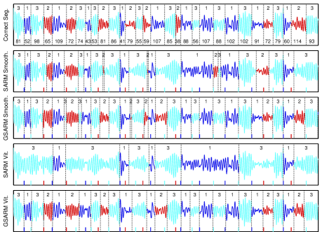
Figure 3.2: Top: Segmentation up to the first 30 regime changes of the time series generated from the switching autoregressive process (3.4.1). The numbers at the top and bottom indicate the regimes and the durations respectively. Bottom: Segmentations obtained with SARM and GSARM using smoothing and extended Viterbi. The correct segmentation is indicated with bars.

We compared the segmentations obtained with a standard switching autoregressive model (SARM) and its explicit-duration extension employing the discretized truncated Gaussian distribution used to generate the time series (GSARM), assuming that the autoregressive coefficients and noise variance were known. SARM used the maximum likelihood values of $\tilde{\pi}$ and $\pi$ estimated using the correct segmentation.

In Figure 3.3(a) we plot the empirical segment-duration distribution (continuous line), the geometric segment-duration distribution implicitly defined in SARM (dashed line), and the segment-duration distribution used in GSARM (dotted line).

The segmentations, obtained by estimating $s^{*}_{t}=\operatorname*{arg\,max}_{s_{t}}\sum_{c_{t}}\gamma^{\sigma_{t}}_{t}$ (smoothing) and $\sigma^{*}_{1:T}=\operatorname*{arg\,max}_{\sigma_{1:T}}p(\sigma_{1:T}|v_{1:T})$ (extended Viterbi), are displayed at the bottom of Figure 3.2. As a measure of segmentation error, we used the discrepancy between the correct and the estimated regimes. SARM gave $30\%$ error with smoothing and $43\%$ error with extended Viterbi, whilst GSARM gave $18\%$ error with smoothing and $25\%$ with extended Viterbi.

In Figure 3.3(b) we plot the empirical segment-duration distributions estimated from the segmentations.

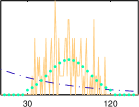
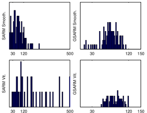
Figure 3.3: (a): Empirical segment-duration distribution (continuous line), geometric segment-duration distribution implicitly defined in SARM (dashed line), and segment-duration distribution used in GSARM (dotted line). (b): Empirical segment-duration distribution of the estimated segmentation for SARM (left) and GSARM (right) using smoothing (top) and extended Viterbi (bottom).

3.4.2 Increasing Count Variables

Figure 3.4: (a): MSM in which the segment-duration distribution is explicitly modelled using increasing count variables $c_{1:T}$. (b): Across-segment independence is enforced with a link from $c_{t}$ to $v_{t}$. (c): Explicit representation of across-segment independence. The values $c_{t+1}=2$ indicates that the segment passing through time-step $t+1$ starts at time-step $t+1-c_{t+1}+1=t$.

Like decreasing count variables, increasing count variables allow Markovian dependence among the observations. For Markovian order $k=1$, this type of models is represented by the belief network shown in Figure 3.4(a). Across-segment independence can be enforced by adding a link from $c_{t}$ to $v_{t}$ (as shown in Figure 3.4(b) and explicitly represented in Figure 3.4(c)), such that $p(v_{t}|\sigma_{t},v_{t-k:t-1})=p(v_{t}|\sigma_{t},v_{t-\min(c_{t},k)+1:t-1})$.

In the following sections we describe inference assuming across-segment independence.

Parallel filtering-smoothing

The filtered distribution $\alpha^{\sigma_{t}}_{t}=p(\sigma_{t}|v_{1:t})$ can be obtained by normalizing $\bar{\alpha}^{\sigma_{t}}_{t}=p(\sigma_{t},v_{1:t})$, where $\bar{\alpha}^{\sigma_{t}}_{t}$ can be computed as

$$\hskip-5.69046pt\bar{\alpha}^{\sigma_{t}}_{t} =p(v_{t}|\sigma_{t},\cancel{v_{1:t-k-1}},v_{t-k:t-1})\sum_{\sigma_{t-1}}p(\sigma_{t}|\sigma_{t-1},\cancel{v_{1:t-1}})p(\sigma_{t-1},v_{1:t-1})$$

$$=e^{\sigma_{t}}_{t}\bigg{\{}\delta_{\begin{subarray}{l}c_{t}>1\\ s_{t-1}=s_{t}\\ c_{t-1}=c_{t}-1\end{subarray}}\hskip-8.5359pt\lambda_{\sigma_{t-1}}\hskip-2.84544pt+\delta_{c_{t}=1}\sum_{s_{t-1}}\pi_{s_{t}s_{t-1}}\hskip 0.0pt\sum_{c_{t-1}}\hskip 0.0pt(1\!-\!\lambda_{\sigma_{t-1}})\bigg{\}}\bar{\alpha}^{\sigma_{t-1}}_{t-1},\hskip-2.84544pt$$ (3.3)

with $e^{\sigma_{t}}_{t}=p(v_{t}|\sigma_{t},v_{t-\min(c_{t},k)+1:t-1})$. With pre-computation of $\sum_{c_{t-1}}(1-\lambda_{\sigma_{t-1}})\bar{\alpha}^{\sigma_{t-1}}_{t-1}$, which does not depend on $s_{t}$, this recursion has cost ${\cal O}(TS(S+Ed_{\max}))$, where $E$ is the cost of computing $e^{\sigma_{t}}_{t}$.

Notice that $\bar{\alpha}^{\sigma_{t}}_{t}=0$ implies $\bar{\alpha}^{s_{t},c_{t}+1}_{t+1}=\ldots=\bar{\alpha}^{s_{t},d_{\max}}_{t+d_{\max}-c_{t}}=0$, i.e. if according to $v_{1:t}$ a segment starting at time-step $t-c_{t}+1$ and generated by $s_{t}$ cannot have duration $\geq c_{t}$, that segment cannot have duration $\geq c_{t}+1$ after incorporating observations $v_{t+1}$, etc. This result can be used to design approximation schemes for reducing the computational cost by pruning some $\bar{\alpha}^{\sigma_{t}}_{t}$, see §3.6.

The smoothed distribution $\gamma^{\sigma_{t}}_{t}=p(\sigma_{t}|v_{1:T})$ can be obtained as $\gamma^{\sigma_{t}}_{t}\propto p(v_{t+1:T}|\sigma_{t},\cancel{v_{1:t-k}},v_{t-k+1:t})p(\sigma_{t},v_{1:t})=\beta^{\sigma_{t}}_{t}\bar{\alpha}^{\sigma_{t}}_{t}$, where $\beta^{\sigma_{t}}_{t}=p(v_{t+1:T}|\sigma_{t},v_{t-k+1:t})$ can be computed as

$$\beta^{\sigma_{t}}_{t}\!=\!\!\sum_{\sigma_{t+1}}\!p(v_{t+1:T}|\cancel{\sigma_{t}},\sigma_{t+1},v_{t-k+1:t})p(\sigma_{t+1}|\sigma_{t},\cancel{v_{t-k+1:t}})$$

$$\!=\!\!\sum_{\sigma_{t+1}}\!p(v_{t+2:T}|\sigma_{t+1},\cancel{v_{t-k+1}},v_{t-k+2:t+1})p(v_{t+1}|\sigma_{t+1},v_{t-k+1:t})p(\sigma_{t+1}|\sigma_{t})$$

$$\!=\!\bigg{\{}\delta_{\begin{subarray}{l}c_{t}<d_{\max}\\ s_{t+1}=s_{t}\\ c_{t+1}=c_{t}+1\end{subarray}}\lambda_{\sigma_{t}}+\delta_{\begin{subarray}{l}c_{t}\geq d_{\min}\\[2.0pt] c_{t+1}=1\end{subarray}}(1\!-\!\lambda_{\sigma_{t}})\sum_{s_{t+1}}\pi_{s_{t+1}s_{t}}\bigg{\}}e^{\sigma_{t+1}}_{t+1}\beta^{\sigma_{t+1}}_{t+1}.$$

With pre-computation of $\sum_{s_{t+1}}\pi_{s_{t+1}s_{t}}e^{s_{t+1},1}_{t+1}\beta^{s_{t+1},1}_{t+1}$, which does not depend on $c_{t}$, this recursion has cost ${\cal O}(TS(S+d_{\max}))$.

Sequential filtering-smoothing

The filtered distribution $\alpha^{\sigma_{t}}_{t}=p(\sigma_{t}|v_{1:t})$ can be obtained as $\alpha^{\sigma_{t}}_{t}=\frac{p(\sigma_{t},v_{t}|v_{1:t-1})}{p(v_{t}|v_{1:t-1})}$, where the numerator can be computed as in recursion (3.3).

The smoothed distribution $\gamma^{\sigma_{t}}_{t}=p(\sigma_{t}|v_{1:T})$ can be computed as

$$\gamma^{\sigma_{t}}_{t}\!=\!\sum_{\sigma_{t+1}}p(\sigma_{t}|\sigma_{t+1},v_{1:t},\cancel{v_{t+1:T}})p(\sigma_{t+1}|v_{1:T})$$ (3.4)

$$\!=\!\delta_{c_{t}<d_{\max}}\gamma^{s_{t},c_{t}+1}_{t+1}\!\!+\delta_{\begin{subarray}{l}c_{t}\geq d_{\min}\\[2.0pt] c_{t+1}=1\end{subarray}}\sum_{s_{t+1}}\frac{p(\sigma_{t+1}|\sigma_{t},\cancel{v_{1:t}})p(\sigma_{t}|v_{1:t})}{\sum_{\tilde{\sigma}_{t}}p(\sigma_{t+1}|\tilde{\sigma}_{t},\cancel{v_{1:t}})p(\tilde{\sigma}_{t}|v_{1:t})}\gamma^{\sigma_{t+1}}_{t+1}$$

$$\!=\!\delta_{c_{t}<d_{\max}}\gamma^{s_{t},c_{t}+1}_{t+1}\!\!+\delta_{\begin{subarray}{l}c_{t}\geq d_{\min}\\[2.0pt] c_{t+1}=1\end{subarray}}(1\!-\!\lambda_{\sigma_{t}})\alpha^{\sigma_{t}}_{t}\!\sum_{s_{t+1}}\frac{\pi_{s_{t+1}s_{t}}\gamma^{\sigma_{t+1}}_{t+1}}{\sum_{\tilde{s}_{t}}\!\pi_{s_{t+1}\tilde{s}_{t}}\sum_{\tilde{c}_{t}}(1\!-\!\lambda_{\tilde{\sigma}_{t}})\alpha^{\tilde{\sigma}_{t}}_{t}},$$

where we have used $p(\sigma_{t}|\sigma_{t+1}=(s_{t},c_{t}+1),v_{1:t})=1$. With pre-summation over $s_{t+1}$, this recursion has cost ${\cal O}(TS(S+d_{\max}))$.

Notice that $\alpha^{\sigma_{t}}_{t}=0$ implies $\gamma^{\sigma_{t}}_{t}=\gamma^{s_{t},c_{t}+1}_{t+1}=\ldots=\gamma^{s_{t},d_{\max}}_{t+d_{\max}-c_{t}}=0$.

Extended Viterbi

With the definition $\xi^{\sigma_{t}}_{t}=\max_{\sigma_{1:t-1}}p(\sigma_{1:t},v_{1:t})$, the most likely sequence $\sigma^{*}_{1:T}=\operatorname*{arg\,max}_{\sigma_{1:T}}p(\sigma_{1:T}|v_{1:T})$ can be obtained as follows:

$$\xi^{\sigma_{1}}_{1}=p(\sigma_{1},v_{1})=\bar{\alpha}^{\sigma_{1}}_{1}$$

$$\textrm{for }t=2,\ldots,T$$

$$\hskip 15.6491pt\textrm{for }c_{t}=1,\ldots,d_{\max}$$

$$\hskip 31.2982pt\xi^{\sigma_{t}}_{t}=\begin{cases}e^{\sigma_{t}}_{t}\max\limits_{s_{t-1}}\pi_{s_{t}s_{t-1}}\max\limits_{c_{t-1}}(1\!-\!\lambda_{\sigma_{t-1}})\xi^{\sigma_{t-1}}_{t-1}&\hskip 15.6491pt\textrm{if }c_{t}\!=\!1\\ e^{\sigma_{t}}_{t}\lambda_{s_{t-1}c_{t}-1}\xi^{s_{t},c_{t}-1}_{t-1}&\hskip 15.6491pt\textrm{if }c_{t}\!>\!1\end{cases}$$

$$\hskip 31.2982pt\psi^{\sigma_{t}}_{t}=\begin{cases}\operatorname*{arg\,max}\limits_{s_{t-1}}\pi_{s_{t}s_{t-1}}\operatorname*{arg\,max}\limits_{c_{t-1}}(1\!-\!\lambda_{\sigma_{t-1}})\xi^{\sigma_{t-1}}_{t-1}&\hskip-5.69046pt\textrm{if }c_{t}\!=\!1\\ (s_{t},c_{t}\!-\!1)&\hskip-5.69046pt\textrm{if }c_{t}\!>\!1\end{cases}$$

$$\sigma^{*}_{T}=\operatorname*{arg\,max}_{\sigma_{T}}\xi^{\sigma_{T}}_{T}$$

$$\textrm{for }t=T\!-\!1,\ldots,1$$

$$\hskip 15.6491pt\sigma^{*}_{t}=\psi^{\sigma^{*}_{t+1}}_{t+1}.$$

3.4.3 Count-Duration Variables

Count-duration variables allow any structure for $p(v_{1:T}|\sigma_{1:T})$ within a segment and therefore, unlike count variables, also a distribution $p(v_{1:T}|\sigma_{1:T})$ that cannot be efficiently computed as $\prod_{t}p(v_{t}|\sigma_{t},v_{1:t-1})$. For models that contain only $\sigma_{1:T}$ and $v_{1:T}$ and with across-segment independence, this translates into non-Markovian dependence between the observations. This type of models is represented by the belief network shown in Figure 3.5(a), where across-segment independence is enforced with a link from $c_{t}$ and $d_{t}$ to $v_{t}$ (explicitly represented in Figure 3.5(b)) and non-Markovian dependence is indicated by undirected links.

Non-Markovian dependence between the observations within a segment is possible as, whilst time-recursive inference cannot be performed in this complex scenario, knowledge about segment beginning and segment end enables segment-recursive inference, namely in terms of count variables that take value 1 and involving the whole segment-emission distribution $e^{s_{t},d_{t}}_{t}=p(v_{t-d_{t}+1:t}|s_{t},d_{t},c_{t}=1)=p(v_{t-d_{t}+1:t}|\sigma_{t-d_{t}+1}=(s_{t},d_{t},d_{t}),\ldots,\sigma_{t-1}=(s_{t},d_{t},2),s_{t},d_{t},c_{t}=1)$.

Figure 3.5: (a): MSM in which the segment-duration distribution is explicitly modelled using decreasing count variables $c_{1:T}$ and duration variables $d_{1:T}$. The undirected links between the observations indicate non-Markovian dependence. Across-segment independence is enforced with a link from $c_{t}$ and $d_{t}$ to $v_{t}$. (b): Explicit representation of across-segment independence. The values $d_{t+1}=3,c_{t+1}=2$ indicate that the segment passing through time-step $t+1$ starts at time-step $t+1-d_{t+1}+c_{t+1}=t$.

The segmental recursions that we describe coincide with the standard recursions of hidden semi-Markov/segment models (Ferguson, 1980; Rabiner, 1989; Ostendorf et al., 1996; Murphy, 2002; Yu, 2010), which are obtained by defining only duration variables and by performing the computations at the occurrence of the events segment end and segment beginning. As discussed above and in Murphy (2002), this approach can be more easily explained by defining also variables $c_{1:T}$ such that, e.g., $c_{t}=1$ at the end of the segment and $c_{t}=2$ otherwise, and by performing inference in terms of time-steps for which $c_{1:T}$ take value 1. These variables can be seen as collapsed count variables that encode information about whether (rather than where) the segment is ending, such that information about segment beginning and segment end is available only at the end of the segment. In this encoding $\sigma_{1:T}$ do not form a first-order Markov chain. Indeed, e.g., $c_{t}$ depends on $d_{t},c_{t-1}$ if $c_{t-1}=1$, whilst it depends on $c_{t-d_{t}+1:t-1}$ if $c_{t-1}=2$.

Encoding information about segment beginning and segment end anywhere within the segment, whilst not having any computational disadvantage, has the advantage of making the derivation of posterior distributions more immediate. This is particularly useful in models with additional unobserved variables related by first-order Markovian dependence, as we will see in §3.5.

In the following sections we describe segmental inference and learning assuming across-segment independence.

Segmental parallel filtering-smoothing

Using the notation $\sigma^{1}_{t}=(s_{t},d_{t},c_{t}=1)$, the filtered distribution $\alpha^{\sigma^{1}_{t}}_{t}=p(\sigma^{1}_{t}|v_{1:t})$ can be obtained by normalizing $\bar{\alpha}^{\sigma^{1}_{t}}_{t}=p(\sigma^{1}_{t},v_{1:t})$, where $\bar{\alpha}^{\sigma^{1}_{t}}_{t}$ can be computed as

$$\bar{\alpha}^{\sigma^{1}_{t}}_{t} =\sum_{\sigma_{t-d_{t}:t-1}}\hskip-5.69046ptp(v_{t-d_{t}+1:t}|\cancel{\sigma_{t-d_{t}}},\sigma_{t-d_{t}+1:t-1},\sigma^{1}_{t},\cancel{v_{1:t-d_{t}}})$$

$$\hskip 17.07182pt\times p(\sigma_{t-d_{t}+1:t-1},\sigma^{1}_{t}|\sigma_{t-d_{t}},\cancel{v_{1:t-d_{t}}})p(\sigma_{t-d_{t}},v_{1:t-d_{t}})$$

$$=e^{s_{t},d_{t}}_{t}\sum_{s_{t-d_{t}},d_{t-d_{t}}}\hskip-5.69046ptp(s_{t-d_{t}+1}\!=\!s_{t}|s_{t-d_{t}},c_{t-d_{t}}\!=\!1)$$

$$\hskip 17.07182pt\times p(d_{t-d_{t}+1}\!=\!d_{t}|d_{t-d_{t}},c_{t-d_{t}}\!=\!1)p(\sigma^{1}_{t-d_{t}},v_{1:t-d_{t}})$$

$$=e^{s_{t},d_{t}}_{t}\rho_{s_{t}d_{t}}\sum_{s_{t-d_{t}}}\pi_{s_{t}s_{t-d_{t}}}\sum_{d_{t-d_{t}}}\bar{\alpha}^{\sigma^{1}_{t-d_{t}}}_{t-d_{t}}.$$ (3.5)

Naive computation of this recursion has cost ${\cal O}(TS^{2}Ed_{\max}^{2})$, where $E$ is the cost of computing $e^{s_{t},d_{t}}_{t}$. However, with pre-computation of $\sum_{d_{t-d_{t}}}\bar{\alpha}^{\sigma^{1}_{t-d_{t}}}_{t-d_{t}}$, which does not depend on $s_{t}$ and $d_{t}$, and with pre-computation of $\sum_{s_{t-d_{t}}}\pi_{s_{t}s_{t-d_{t}}}\sum_{d_{t-d_{t}}}\bar{\alpha}^{\sigma^{1}_{t-d_{t}}}_{t-d_{t}}$, which does not depend on $d_{t}$, the cost reduces to ${\cal O}(TS(S+Ed_{\max}))$.

In the case of Markovian dependence between the observations, if $\bar{\alpha}^{\sigma_{t}}_{t}$ for $c_{t}>1$ is of interest, a time-recursive routine on the line of the one described in Appendix A.5 for $\alpha^{\sigma_{t}}_{t}$ can be used.

The smoothed distribution $\gamma^{\sigma^{1}_{t}}_{t}=p(\sigma^{1}_{t}|v_{1:T})$ can be obtained as $\gamma^{\sigma^{1}_{t}}_{t}\propto p(v_{t+1:T}|s_{t},\cancel{d_{t}},c_{t}\!=\!1,\cancel{v_{1:t}})p(\sigma^{1}_{t},v_{1:t})=\beta^{s_{t},1}_{t}\bar{\alpha}^{\sigma^{1}_{t}}_{t}$, where, with the notation $\sigma^{j,k,1}_{t+k}=(s_{t+k}=j,d_{t+k}=k,c_{t+k}=1)$, $\beta^{s_{t},1}_{t}=p(v_{t+1:T}|s_{t},c_{t}=1)$ can be computed as

$$\beta^{s_{t},1}_{t} =\!\sum_{j,k}\!p(v_{t+1:T}|\sigma^{j,k,1}_{t+k},\cancel{s_{t},c_{t}\!=\!1})p(\sigma^{j,k,1}_{t+k}|s_{t},c_{t}\!=\!1)$$

$$=\!\sum_{j,k}\!p(v_{t+1:t+k}|\sigma^{j,k,1}_{t+k},\cancel{v_{t+k+1:T}})p(v_{t+k+1:T}|\sigma^{j,k,1}_{t+k})\pi_{js_{t}}\rho_{jk}$$

$$=\!\sum_{j}\!\pi_{js_{t}}\sum_{k}p(v_{t+1:t+k}|\sigma^{j,k,1}_{t+k})\beta^{j,1}_{t+k}\rho_{jk}.$$ (3.6)

With pre-computation of $\sum_{k}p(v_{t+1:t+k}|\sigma^{j,k,1}_{t+k})\beta^{j,1}_{t+k}\rho_{jk}$, this recursion has cost ${\cal O}(TS(S+d_{\max}))$.

Notice that recursions (3.5) and (3.6) correspond to the standard recursions of hidden semi-Markov/segment models using collapsed count variables (Ferguson, 1980; Rabiner, 1989; Ostendorf et al., 1996; Murphy, 2002; Yu, 2010).

The smoothed distribution $\gamma^{\sigma_{t}}_{t}$ for $c_{t}>1$ can be obtained as $\gamma^{\sigma_{t}}_{t}=\gamma^{s_{t},d_{t},1}_{t+c_{t}-1}$. Indeed, in such a case,

$$\gamma^{\sigma_{t}}_{t} =\sum_{\sigma_{t+1}}p(\sigma_{t}|\sigma_{t+1},v_{1:t},\cancel{v_{t+1:T}})p(\sigma_{t+1}|v_{1:T})$$

$$=\gamma^{s_{t},d_{t},c_{t}-1}_{t+1}=\gamma^{s_{t},d_{t},c_{t}-2}_{t+2}=\cdots=\gamma^{s_{t},d_{t},1}_{t+c_{t}-1},$$ (3.7)

where we have used $p(\sigma_{t}|\sigma_{t+1}=(s_{t},d_{t},c_{t}-1),v_{1:t})=1$.

From Equation (3.7) we can immediately derive $p(s_{t},c_{t}|v_{1:T})$ and $p(s_{t}|v_{1:T})$ as

$$p(s_{t},c_{t}|v_{1:T})=\sum_{d_{t}=\max(d_{\min},c_{t})}^{d_{\max}}\gamma^{\sigma_{t}}_{t}=\sum_{d_{t}}\gamma^{s_{t},d_{t},1}_{t+c_{t}-1}\propto\beta^{s_{t},1}_{t+c_{t}-1}\sum_{d_{t}}\bar{\alpha}^{s_{t},d_{t},1}_{t+c_{t}-1},$$

and

$$\hskip-5.69046ptp(s_{t}|v_{1:T})=\sum_{c_{t}=1}^{d_{\max}}p(s_{t},c_{t}|v_{1:T})\propto\sum_{\tau=t}^{t+d_{\max}-1}\beta^{s_{t},1}_{\tau}\hskip-8.5359pt\sum_{d_{t}=\max(d_{\min},\tau-t+1)}^{d_{\max}}\hskip-19.91684pt\bar{\alpha}^{s_{t},d_{t},1}_{\tau}.\hskip-2.84544pt$$ (3.8)

In the standard approach that uses collapsed count variables, $p(s_{t}|v_{1:T})$ is derived by observing that the set of all segments passing through time-step $t$ needs to be considered, and that this set can be obtained by subtracting all segments ending before time-step $t$ from all segments starting at time-step $t$ or before (see Appendix A.5). In Equation (3.8), $p(s_{t}|v_{1:T})$ is computed by summing over all segments passing through time-step $t$, which are obtained as all segments that start at time-step $t$ or before and end at time-step $t$ or after. However, the equation was derived by use of equivalence (3.7) rather than by use of this observation. Therefore, uncollapsed count variables enable more automatic derivations of posterior distributions of interest.

Segmental sequential filtering-smoothing

The filtered distribution $\alpha^{\sigma^{1}_{t}}_{t}=p(\sigma^{1}_{t}|v_{1:t})$ can be obtained as $\alpha^{\sigma^{1}_{t}}_{t}=\frac{p(\sigma^{1}_{t},v_{t-d_{t}+1:t}|v_{1:t-d_{t}})}{p(v_{t-d_{t}+1:t}|v_{1:t-d_{t}})}$, where the numerator can be computed as in recursion (3.5).

The smoothed distribution $\gamma^{\sigma^{1}_{t}}_{t}=p(\sigma^{1}_{t}|v_{1:T})$ can be computed as

$$\gamma^{\sigma^{1}_{t}}_{t} =\sum_{s_{t+1},d_{t+1}}\frac{\pi_{s_{t+1}s_{t}}\cancel{\rho_{s_{t+1}d_{t+1}}}\alpha^{\sigma^{1}_{t}}_{t}}{\sum_{\tilde{s}_{t},\tilde{d}_{t}}\pi_{s_{t+1}\tilde{s}_{t}}\cancel{\rho_{s_{t+1}d_{t+1}}}\alpha^{\tilde{\sigma}^{1}_{t}}_{t}}\gamma^{s_{t+1},d_{t+1},d_{t+1}}_{t+1}$$

$$=\alpha^{\sigma^{1}_{t}}_{t}\sum_{s_{t+1}}\frac{\pi_{s_{t+1}s_{t}}}{\sum_{\tilde{s}_{t}}\pi_{s_{t+1}\tilde{s}_{t}}\sum_{\tilde{d}_{t}}\alpha^{\tilde{\sigma}^{1}_{t}}_{t}}\sum_{d_{t+1}}\gamma^{s_{t+1},d_{t+1},1}_{t+d_{t+1}}.$$ (3.9)

With pre-summation over $k$ and $j$, the cost of this recursion is ${\cal O}(TS(S+d_{\max}))$.

Segmental extended Viterbi

With the definition $\xi^{\sigma^{1}_{t}}_{t}=\max_{s_{1:t-1},d_{1:t-1}}p(s_{1:t-1},d_{1:t-1},\sigma^{1}_{t},v_{1:t})$, the most likely sequence $\sigma^{*}_{1:T}=\operatorname*{arg\,max}_{\sigma_{1:T}}p(\sigma_{1:T}|v_{1:T})$ can be computed as follows (assuming $c^{*}_{T}=1$):

$$\textrm{for }t=1,\ldots,T$$

$$\hskip 8.5359pt\left.\begin{array}[]{l}\xi^{\sigma^{1}_{t}}_{t}=p(v_{t-d_{t}+1:t}|\sigma^{1}_{t})\rho_{s_{t}d_{t}}\max\limits_{s_{t-d_{t}}}\pi_{s_{t}s_{t-d_{t}}}\max\limits_{d_{t-d_{t}}}\xi^{\sigma^{1}_{t-d_{t}}}_{t-d_{t}}\\ \psi^{s_{t},d_{t}}_{t}=\operatorname*{arg\,max}\limits_{s_{t-d_{t}},d_{t-d_{t}}}\pi_{s_{t}s_{t-d_{t}}}\xi^{\sigma^{1}_{t-d_{t}}}_{t-d_{t}}\end{array}\right.$$

$$\sigma^{*}_{T}=(\operatorname*{arg\,max}\limits_{s_{T},d_{T}}\xi^{\sigma^{1}_{T}}_{T},1)$$

$$s^{*}_{T-d^{*}_{T}+1:T-1}=s^{*}_{T},\hskip 5.69046ptd^{*}_{T-d^{*}_{T}+1:T-1}=d^{*}_{T},\hskip 5.69046ptc^{*}_{T-d^{*}_{T}+1:T-1}=d^{*}_{T},\ldots,2$$

$$t=T\!-\!d^{*}_{T}$$

$$\textrm{while }t\!\geq\!1$$

$$\hskip 15.6491pt\left.\begin{array}[]{l}\sigma^{*}_{t}=(\psi^{s^{*}_{t+1},d^{*}_{t+1}}_{t+1},1)\\ s^{*}_{t-d^{*}_{t}+1:t-1}=s^{*}_{t},\hskip 5.69046ptd^{*}_{t-d^{*}_{t}+1:t-1}=d^{*}_{t},\hskip 5.69046ptc^{*}_{t-d^{*}_{t}+1:t-1}=d^{*}_{t},\ldots,2\\ t=t-d^{*}_{t}\,.\end{array}\right.$$

Segmental learning

In this section we show how count-duration variables enable to derive EM updates in a straightforward way. The relation with the standard approach that uses collapsed count variables is given in Appendix A.5.

The expectation of the complete data log-likelihood can be written as

$${\cal L} =\sum_{t=1}^{T}\sum_{d_{t}}\gamma^{\sigma^{1}_{t}}_{t}\log p(v_{t-d_{t}+1:t}|\sigma^{1}_{t})$$

$$+\sum_{s_{1}}p(s_{1}|v_{1:T})\log\tilde{\pi}_{s_{1}}+\sum_{t=2}^{T}\sum_{s_{t-1},s_{t}}p(s_{t-1},c_{t-1}\!=\!1,s_{t}|v_{1:T})\log\pi_{s_{t}s_{t-1}}$$

$$+\sum_{s_{1},d_{1}}p(s_{1},d_{1}|v_{1:T})\log\tilde{\rho}_{s_{1}d_{1}}+\sum_{t=2}^{T}\sum_{s_{t},d_{t}}p(c_{t-1}\!=\!1,s_{t},d_{t}|v_{1:T})\log\rho_{s_{t}d_{t}},$$

giving update for $\rho_{s_{t}d_{t}}$

$$\rho_{s_{t}d_{t}}=\frac{\sum_{t}p(c_{t-1}\!=\!1,s_{t},d_{t}|v_{1:T})}{\sum_{t}\sum_{\tilde{d}_{t}}p(c_{t-1}\!=\!1,s_{t},\tilde{d}_{t}|v_{1:T})}=\frac{\sum_{t}\gamma^{s_{t},d_{t},1}_{t+d_{t}-1}}{\sum_{t}\sum_{\tilde{d}_{t}}\gamma^{s_{t},\tilde{d}_{t},1}_{t+\tilde{d}_{t}-1}},$$ (3.10)

as

$$p(c_{t-1}\!=\!1,s_{t},d_{t}|v_{1:T}) =\cancel{\frac{\sum_{s_{t-1},d_{t-1}}\pi_{s_{t}s_{t-1}}\rho_{s_{t}d_{t}}\alpha^{\sigma^{1}_{t-1}}_{t-1}}{\sum_{\tilde{s}_{t-1},\tilde{d}_{t-1}}\pi_{s_{t}\tilde{s}_{t-1}}\rho_{s_{t}d_{t}}\alpha^{\tilde{\sigma}^{1}_{t-1}}_{t-1}}}\gamma^{s_{t},d_{t},d_{t}}_{t}=\gamma^{s_{t},d_{t},1}_{t+d_{t}-1},$$

and update for $\pi_{s_{t}s_{t-1}}$

$$\pi_{s_{t}s_{t-1}}=\frac{\sum_{t}p(s_{t-1},c_{t-1}\!=\!1,s_{t}|v_{1:T})}{\sum_{t}\sum_{\tilde{s}_{t}}p(s_{t-1},c_{t-1}\!=\!1,\tilde{s}_{t}|v_{1:T})},$$ (3.11)

where

$$\hskip-5.69046ptp(s_{t-1},c_{t-1}\!=\!1,s_{t}|v_{1:T}) =\frac{\pi_{s_{t}s_{t-1}}\sum_{d_{t-1}}\alpha^{\sigma^{1}_{t-1}}_{t-1}}{\sum_{\tilde{s}_{t-1}}\pi_{s_{t}\tilde{s}_{t-1}}\sum_{\tilde{d}_{t-1}}\alpha^{\tilde{\sigma}^{1}_{t-1}}_{t-1}}\sum_{d_{t}}\gamma^{s_{t},d_{t},1}_{t+d_{t}-1}.$$ (3.12)

3.5 Explicit-Duration SLGSSM

Figure 3.6: Belief network representation of the switching linear Gaussian state-space model.

In §3.4 we have seen that the cost of inference in explicit-duration MSMs of type $p(\sigma_{1:T},v_{1:T})$ does not depend on the type of explicit-duration variables used. This is not the case in models that contain additional unobserved variables $h_{1:T}$ related by Markovian dependence, for which inference is more complex.

In this section we consider the most popular of such models, namely the switching linear Gaussian state-space model (SLGSSM), also called switching linear dynamical system (Barber, 2006).

In the SLGSSM, $v_{t}\in\mathbb{R}^{V}$, $h_{t}\in\mathbb{R}^{H}$, and the joint distribution of all variables $p(s_{1:T},h_{1:T},v_{1:T})$ factorizes as

$$p(v_{1}|h_{1},s_{1})p(h_{1}|s_{1})p(s_{1})\prod_{t=2}^{T}p(v_{t}|h_{t},s_{t})p(h_{t}|h_{t-1},s_{t})p(s_{t}|s_{t-1}),$$

giving the belief network representation shown in Figure 3.6. The factors are defined as

$$p(s_{1})=\tilde{\pi}_{s_{1}},\hskip 8.5359ptp(s_{t}|s_{t-1})=\pi_{s_{t}s_{t-1}},$$

$$p(h_{1}|s_{1})={\cal N}(h_{1};\mu^{s_{1}},\Sigma^{s_{1}}),\hskip 8.5359ptp(h_{t}|h_{t-1},s_{t})={\cal N}(h_{t};A^{s_{t}}h_{t-1},\Sigma^{s_{t}}_{H}),$$

$$p(v_{t}|h_{t},s_{t})={\cal N}(v_{t};B^{s_{t}}h_{t},\Sigma^{s_{t}}_{V}),$$

where $\mu^{s_{1}}$ is a $H$-dimensional vector, $\Sigma^{s_{1}}$, $A^{s_{t}}$ and $\Sigma^{s_{t}}_{H}$ are $H\times H$-dimensional matrices, $B^{s_{t}}$ is a $V\times H$-dimensional matrix, and $\Sigma^{s_{t}}_{V}$ is a $V\times V$-dimensional matrix. The model can be equivalently defined by the following linear equations:

$$h_{t}=A^{s_{t}}h_{t-1}+\eta^{h}_{t},\hskip 5.69046pt\eta^{h}_{t}\sim{\cal N}(\eta^{h}_{t};0,\Sigma^{s_{t}}_{H}),\hskip 1.42271pth_{1}\sim{\cal N}(h_{1};\mu^{s_{t}},\Sigma^{s_{t}}),$$ (3.13)

$$v_{t}=B^{s_{t}}h_{t}+\eta^{v}_{t},\hskip 5.69046pt\eta^{v}_{t}\sim{\cal N}(\eta^{v}_{t};0,\Sigma^{s_{t}}_{V}).$$ (3.14)

Performing inference in the SLGSSM requires approximations since, e.g., $p(h_{t}|v_{1:t})$ is a Gaussian mixture with $S^{t}$ components. In the expectation-correction (EC) approach of Barber (2006), the filtered distribution $p(h_{t},s_{t}|v_{1:t})$ is first computed by forming separate recursions for $p(h_{t}|s_{t},v_{1:t})$ and $p(s_{t}|v_{1:t})$, and then used to compute the smoothed distribution $p(h_{t},s_{t}|v_{1:T})$ by forming separate recursions for $p(h_{t}|s_{t},v_{1:T})$ and $p(s_{t}|v_{1:T})$. The recursions are similar to the sequential filtering-smoothing recursions used in §2.2.1. The explosion of mixture components with time is addressed by collapsing, at each time-step, the obtained Gaussian mixture to a Gaussian mixture with a lower number of components (Alspach and Sorenson, 1972). In addition to Gaussian collapsing, EC introduces one approximation in the recursion for $p(h_{t}|s_{t},v_{1:T})$, due to lack of knowledge about the regime at the previous time-step, and one approximation in the recursion for $p(s_{t}|v_{1:T})$. The resulting routines for $p(h_{t}|s_{t},v_{1:t})$ and $p(h_{t}|s_{t},v_{1:T})$ resemble the standard predictor-corrector filtering routines and Rauch-Tung-Striebel smoothing routines of the linear Gaussian state-space model (LGSSM) (Rauch et al., 1965; Grewal and Andrews, 1993; Chiappa, 2006).

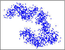
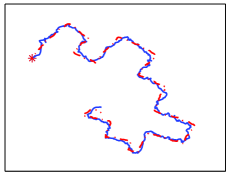
Figure 3.7: (a): Noisy measurements of the positions of a two-wheeled robot moving in the two-dimensional space generated from model (A.4). (b): Actual positions (dashed line) and estimated positions (continuous line) by a SLGSSM (means of $p(h_{t}|v_{1:T})$). The initial position is indicated with a star.

The SLGSSM enables sophisticated modelling and estimation of hidden dynamics underlying noisy observations (Pavlovic et al., 2001; Zoeter, 2005; Mesot and Barber, 2007; Chiappa, 2008; Quinn et al., 2009). It can can be used, e.g., to solve the robot localization problem discussed in Chapter 1, namely to infer the positions of a two-wheeled robot moving in the two-dimensional space plotted in Figure 3.7(b) with a dashed line from the noisy measurements plotted in Figure 3.7(a). As explained in detail in Appendix A.4, the hidden dynamics and observation process can be formulated as a SLGSSM with nonlinear hidden dynamics. The means of $p(h_{t}|v_{1:T})$, computed by combining EC with an unscented approximation (Särkkä, 2008), give reasonably accurate estimates of the positions, as shown in Figure 3.7(b) with a continuous line.

In the SLGSSM, all three approaches to explicit-duration modelling can be used (as the Markovian structure of $h_{1:T}$ enables recursive computation of $p(v_{t}|\sigma_{t},v_{1:t-1})$) and allow $p(v_{1:T}|\sigma_{1:T})$ to factorize across segments. Following closely EC, we describe a sequential filtering-smoothing approach that allows to generalize the results to similar models with unobserved variables related by first-order Markovian dependence. In this approach, the filtered distribution $p(h_{t},\sigma_{t}|v_{1:t})$ is first computed by forming separate recursions for $\hat{\alpha}^{\sigma_{t}}_{t}=p(h_{t}|\sigma_{t},v_{1:t})$ and $\alpha^{\sigma_{t}}_{t}=p(\sigma_{t}|v_{1:t})$, and then used to compute the smoothed distribution $p(h_{t},\sigma_{t}|v_{1:T})$ by forming separate recursions $\hat{\gamma}^{\sigma_{t}}_{t}=p(h_{t}|\sigma_{t},v_{1:T})$ and $\gamma^{\sigma_{t}}_{t}=p(\sigma_{t}|v_{1:T})$.

To gain some intuition about the differences between the three approaches, we can observe that inference on $h_{1:T}$ needs to consider all possible segmentations, i.e. all possible partitioning of the time series into segments and, for each partitioning, all possible combinations of regimes.

In the across-segment-independence case, inference on $h_{1:T}$ given a segmentation reduces to inference in a separate LGSSM for each segment and regime. Since the set of unique segments generated by all possible segmentations is $\{v_{t:t+d_{t}-1},\forall t,\forall d_{t}\}$, only LGSSM filtering-smoothing on segment $v_{t:t+d_{t}-1}$ for each $t$, $s_{t}$ and $d_{t}$ is required. Furthermore, as filtering can be shared between all segments that start at the same time-step and are generated from the same regime, only LGSSM filtering on segment $v_{t:t+d_{\max}-1}$ for each $t$ and $s_{t}$ is required. Therefore, the computational cost of inference on $h_{1:T}$ for all possible segmentations is ${\cal O}(TSd_{\max})$ for filtering and ${\cal O}(TSd^{2}_{\max})$ for smoothing. Computing $p(h_{t}|s_{t},v_{1:t})$ requires to sum over all possible starts of the segment passing through time-step $t$, giving rise to a Gaussian mixture with $d_{\max}$ components. This means that, regardless of the explicit-duration encoding used, $p(h_{t}|s_{t},v_{1:t})$ cannot be simpler than a Gaussian mixture with $d_{\max}$ components. Similarly, computing $p(h_{t}|s_{t},v_{1:T})$ requires to sum over all possible starts and ends of the segment passing through time-step $t$, giving rise to a Gaussian mixture with number of components (of order) $d^{2}_{\max}$. Therefore, $p(h_{t}|s_{t},v_{1:T})$ cannot be simpler than a Gaussian mixture with number of components (of order) $d^{2}_{\max}$. If knowledge about segment beginning is explicitly encoded in the explicit-duration variables, $\hat{\alpha}^{\sigma_{t}}_{t}$ is a Gaussian distribution, and the mixture in $p(h_{t}|s_{t},v_{1:t})$ arises from summing over the explicit-duration variables. If knowledge about segment beginning is not explicitly encoded in the explicit-duration variables, $\hat{\alpha}^{\sigma_{t}}_{t}$ is a Gaussian mixture with (maximally, as segment end is encoded in this case) $d_{\max}$ components. Similarly, $\hat{\gamma}^{\sigma_{t}}_{t}$ is a Gaussian distribution if knowledge about both segment beginning and segment end is explicitly encoded in the explicit-duration variables, and a Gaussian mixture with maximally $d_{\max}$ components otherwise.

Decreasing count variables encode information about segment end. The recursion for $\hat{\alpha}^{\sigma_{t}}_{t}$ (recursion (3.20)) produces a Gaussian mixture with maximally $d_{\max}$ components accounting for all possible segment starts, and therefore has computational cost ${\cal O}(TSd^{2}_{\max})$. The cost can be reduced to ${\cal O}(TSd_{\max})$ with Gaussian collapsing. The recursion for $\hat{\gamma}^{\sigma_{t}}_{t}$ (recursion (3.24)) does not increase the number of components, as segment end is known. Without Gaussian collapsing of $\hat{\alpha}^{\sigma_{t}}_{t}$, the cost of the recursion is therefore ${\cal O}(TSd^{2}_{\max})$. With Gaussian collapsing of $\hat{\alpha}^{\sigma_{t}}_{t}$, the cost is reduced to ${\cal O}(TSd_{\max})$; however, as knowledge about segment beginning is lost, the EC approximation $p(h_{t+1}|s_{t},c_{t}>1,\sigma_{t+1},v_{1:T})\approx\hat{\gamma}^{\sigma_{t+1}}_{t+1}$ in Equation (3.22) is required.

Increasing count variables encode information about segment beginning. The recursion for $\hat{\alpha}^{\sigma_{t}}_{t}$ (recursion (3.26)) produces a Gaussian distribution, and therefore has cost ${\cal O}(TSd_{\max})$. This recursion essentially performs LGSSM filtering on segment $v_{t:t+d_{\max}-1}$ for each $t$ and $s_{t}$. The recursion for $\hat{\gamma}^{\sigma_{t}}_{t}$ (recursion (3.28)) produces a Gaussian mixture with maximally $d_{\max}$ components, which accounts for all possible segment ends, and therefore has cost ${\cal O}(TSd^{2}_{\max})$. The cost can be reduced to ${\cal O}(TSd_{\max})$ with Gaussian collapsing.

Count-duration variables encode information about both segment beginning and segment end. The estimation of $\hat{\alpha}^{\sigma_{t}}_{t}$ and $\hat{\gamma}^{\sigma_{t}}_{t}$ can be recast into filtering and smoothing in a LGSSM, and therefore has cost ${\cal O}(TSd_{\max})$ and ${\cal O}(TSd^{2}_{\max})$ respectively. Alternatively, the estimation can be achieved with time-recursive routines that produce Gaussian distributions and have the same cost (recursions (A.8) and (A.10)). The cost ${\cal O}(TSd_{\max})$ rather than ${\cal O}(TSd^{2}_{\max})$ in the recursion for $\hat{\alpha}^{\sigma_{t}}_{t}$ is achieved by taking care of redundancies.

Decreasing Count Variables	$\hat{\alpha}^{\sigma_{t}}_{t}$	$\alpha^{\sigma_{t}}_{t}$
	GM with maximally $d_{\max}$ components: ${\cal O}(TSd_{\max}^{2})$	${\cal O}(TS^{2}d_{\max})$
	Gaussian collapsing: ${\cal O}(TSd_{\max})$
	$\hat{\gamma}^{\sigma_{t}}_{t}$	$\gamma^{\sigma_{t}}_{t}$
	GM with maximally $d_{\max}$ components: ${\cal O}(TSd_{\max}^{2})$
	Gaussian collapsing of $\alpha^{\sigma_{t}}_{t}$: ${\cal O}(TSd_{\max})$	${\cal O}(TS^{2}d_{\max})$
	$p(h_{t+1}|s_{t},c_{t}>1,\sigma_{t+1},v_{1:T})\approx\hat{\gamma}^{\sigma_{t+1}}_{t+1}$
Increasing Count Var.	$\hat{\alpha}^{\sigma_{t}}_{t}$	$\alpha^{\sigma_{t}}_{t}$
	Gaussian: ${\cal O}(TSd_{\max})$	${\cal O}(TS^{2}d_{\max})$
	$\hat{\gamma}^{\sigma_{t}}_{t}$	$\gamma^{\sigma_{t}}_{t}$
	GM with maximally $d_{\max}$ components: ${\cal O}(TSd_{\max}^{2})$	${\cal O}(TS^{2}d_{\max})$
	Gaussian collapsing: ${\cal O}(TSd_{\max})$
Count-Duration Var.	$\hat{\alpha}^{\sigma_{t}}_{t}$	$\alpha^{\sigma_{t}}_{t}$
	Gaussian: ${\cal O}(TSd_{\max})$	${\cal O}(TS^{2}d_{\max})$
	$\hat{\gamma}^{\sigma_{t}}_{t}$	$\gamma^{\sigma_{t}}_{t}$
	Gaussian: ${\cal O}(TSd_{\max}^{2})$	${\cal O}(TS^{2}d_{\max})$

Table 3.1: Characteristics of the different encodings for the explicit-duration SLGSSM with across-segment independence. GM indicates Gaussian mixture.

In all three approaches, the estimation of $\alpha^{\sigma_{t}}_{t}$ and $\gamma^{\sigma_{t}}_{t}$ has cost ${\cal O}(TS^{2}d_{\max})$. The computation of $\alpha^{\sigma_{t}}_{t}$ requires filtering on $h_{1:T}$ and, if decreasing count variables are used, the computation of $\gamma^{\sigma_{t}}_{t}$ requires smoothing on $h_{1:T}$.

In summary, increasing count variables and count-duration variables have the advantage over decreasing count variables of requiring only filtering on $h_{1:T}$ to perform segmentation. Without Gaussian collapsing, increasing count variables and count-duration variables give the same computational cost. They are advantageous over decreasing count variables as filtering on $h_{1:T}$ has lower cost and as smoothing on $h_{1:T}$ is simpler. The count-duration-variable approach is more intuitive than the increasing-count-variable approach. However, increasing count variables do not require taking care of redundancies. With Gaussian collapsing, which can be performed in filtering with decreasing count variables and in smoothing with increasing count variables, count variables give that same computational cost, which is lower in smoothing on $h_{1:T}$ than with count-duration variables. However, decreasing count variables require the EC approximation $p(h_{t+1}|s_{t},c_{t}>1,\sigma_{t+1},v_{1:T})\approx\hat{\gamma}^{\sigma_{t+1}}_{t+1}$ in Equation (3.22). In similar models in which $h_{1:T}$ are discrete, similar conclusions to the Gaussian collapsing case can be made. The characteristics are summarized in Table 3.1.

In the across-segment-dependence case, explicit-duration modelling increases the computational complexity with respect to the standard SLGSSM, and therefore Gaussian collapsing is required. If time-step $t$ corresponds to the beginning of a segment, $c_{t-1}$ must have value 1 in the decreasing-count-variable approach and can take any value in the increasing-count-variable approach. This means that the recursion for $\hat{\alpha}^{\sigma_{t}}_{t}$ using decreasing count variables (recursion (3.15)) produces a Gaussian mixture with less components than the recursion for $\hat{\alpha}^{\sigma_{t}}_{t}$ using increasing count variables (recursion (3.25)). The reverse happens in the recursion for $\hat{\gamma}^{\sigma_{t}}_{t}$ (recursions (3.21) and (3.27)). Count-duration variables (requiring time-recursive inference) give rise to more complex Gaussian mixtures than count variables. Gaussian collapsing reduces the cost of the recursions for $\hat{\alpha}^{\sigma_{t}}_{t}$, and $\hat{\gamma}^{\sigma_{t}}_{t}$ to ${\cal O}(TS^{2}d_{\max})$ in the count-variable approaches and to ${\cal O}(TS^{2}d^{2}_{\max})$ in the count-duration-variable approach. The computation of $\alpha^{\sigma_{t}}_{t}$ and $\gamma^{\sigma_{t}}_{t}$ has cost ${\cal O}(TS^{2}d_{\max})$ in all approaches. Unlike decreasing count variables, increasing count variables and count-duration variables require the EC approximations only for $c_{t}=1$. In similar models with discrete unobserved variables related by first-order Markovian dependence, similar conclusions to the Gaussian collapsing case can be made.

Therefore, the increasing count variable approach is overall preferable in both the across-segment-independence and across-segment-dependence cases.

In the following sections we describe the three approaches in more detail.

The explicit-duration SLGSSM is also discussed in Oh et al. (2008) using increasing count variables and in Bracegirdle and Barber (2011) and Bracegirdle (2013) in the context of reset models (see §3.6). Bracegirdle and Barber (2011) and Bracegirdle (2013) present a recursion for $\hat{\alpha}^{\sigma_{t}}_{t}$ using increasing count variables that is equivalent to recursion (3.26), and a recursion for $\hat{\gamma}^{\sigma_{t}}_{t}$ using increasing-decreasing count variables with cost ${\cal O}(TSd^{2}_{\max})$. Increasing-decreasing count variables provide the same information as count-duration variables but give rise to more convoluted recursions. The computation of the smoothed distributions in the increasing-decreasing-count-variable representation using filtered distributions computed in the increasing-count-variable representation is possible as across-segment-dependence is cut.

3.5.1 Decreasing Count Variables

The explicit-duration SLGSSM using decreasing count variables has belief network representation given in Figure 3.8(a). Across-segment independence can be enforced by adding a link from $c_{t}$ to $h_{t+1}$, as in Figure 3.8(b), which has the effect of removing the link from $h_{t}$ to $h_{t+1}$ if $c_{t}=1$, as explicitly represented in Figure 3.8(c). More specifically, dependence cut is defined as

$$p(h_{t}|h_{t-1},c_{t-1},s_{t}) =\begin{cases}p(h_{t}|c_{t-1},s_{t})={\cal N}(h_{t};\mu^{s_{t}},\Sigma^{s_{t}})&\textrm{if }c_{t-1}\!=\!1\\ {\cal N}(h_{t};A^{s_{t}}h_{t-1},\Sigma^{s_{t}}_{H})&\textrm{if }c_{t-1}\!>\!1.\end{cases}$$

Filtering

Figure 3.8: (a): Explicit-duration SLGSSM using decreasing count variables. (b): Across-segment independence is enforced with a link from $c_{t}$ to $h_{t+1}$, as explicitly represented in (c).

To compute the filtered distribution $p(h_{t},\sigma_{t}|v_{1:t})$, we form separate recursions for $\alpha^{\sigma_{t}}_{t}=p(\sigma_{t}|v_{1:t})$ and $\hat{\alpha}^{\sigma_{t}}_{t}=p(h_{t}|\sigma_{t},v_{1:t})$.

The recursion for $\alpha^{\sigma_{t}}_{t}$ is given by

$$\alpha^{\sigma_{t}}_{t} =\frac{\sum_{\sigma_{t-1}}p(\sigma_{t-1:t},v_{t}|v_{1:t-1})}{\sum_{\tilde{\sigma}_{t-1:t}}p(\tilde{\sigma}_{t-1:t},v_{t}|v_{1:t-1})}$$

$$\propto\sum_{\sigma_{t-1}}p(v_{t}|\sigma_{t-1},s_{t},\cancel{c_{t}},v_{1:t-1})p(\sigma_{t}|\sigma_{t-1},\cancel{v_{1:t-1}})p(\sigma_{t-1}|v_{1:t-1})$$

$$=\bigg{\{}\delta_{\begin{subarray}{l}c_{t}<d_{\max}\\ s_{t-1}=s_{t}\\ c_{t-1}=c_{t}+1\end{subarray}}+\delta_{\begin{subarray}{l}c_{t}\geq d_{\min}\\ c_{t-1}=1\end{subarray}}\rho_{\sigma_{t}}\sum_{s_{t-1}}\pi_{s_{t}s_{t-1}}\bigg{\}}e^{\sigma_{t-1},s_{t}}_{t}\alpha^{\sigma_{t-1}}_{t-1},$$

where (see Equation (3.17) below) $e^{\sigma_{t-1},s_{t}}_{t}=p(v_{t}|\sigma_{t-1},s_{t},v_{1:t-1})={\cal N}(v_{t};B^{s_{t}}\hat{h}_{t}^{t-1,\sigma_{t-1},s_{t}},B^{s_{t}}P_{t}^{t-1,\sigma_{t-1},s_{t}}(B^{s_{t}})^{\textsf{T}}+\Sigma^{s_{t}}_{V})$, with the symbol ${}^{\textsf{T}}$ denoting the transpose operator. Notice that $v_{t}\cancel{\perp\!\!\!\perp}c_{t-1}|\{s_{t-1:t},v_{1:t-1}\}$ as the path $c_{t-1},c_{t-2},s_{t-2},h_{t-2:t},v_{t}$ in Figure 3.8(a) is not blocked. This recursion has computational cost ${\cal O}(TS^{2}d_{\max})$.

The recursion for $\hat{\alpha}^{\sigma_{t}}_{t}$ is given by

$$\hat{\alpha}^{\sigma_{t}}_{t}=\sum_{\sigma_{t-1}}p(h_{t}|\sigma_{t-1},s_{t},\cancel{c_{t}},v_{1:t})p(\sigma_{t-1}|\sigma_{t},v_{1:t})$$ (3.15)

$$\!=\!\sum_{\sigma_{t-1}}p(h_{t}|\sigma_{t-1},s_{t},v_{1:t})\frac{p(\sigma_{t-1:t},v_{t}|v_{1:t-1})}{\sum_{\tilde{\sigma}_{t-1}}p(\tilde{\sigma}_{t-1},\sigma_{t},v_{t}|v_{1:t-1})}$$

$$\!=\!\frac{1}{n^{\sigma_{t}}_{t}}\bigg{\{}\delta_{\begin{subarray}{l}c_{t}<d_{\max}\\ s_{t-1}=s_{t}\\ c_{t-1}=c_{t}+1\end{subarray}}\hskip-11.38092pt+\delta_{\begin{subarray}{l}c_{t}\geq d_{\min}\\ c_{t-1}=1\end{subarray}}\rho_{\sigma_{t}}\hskip 0.0pt\sum_{s_{t-1}}\hskip 0.0pt\pi_{s_{t}s_{t-1}}\bigg{\}}e^{\sigma_{t-1},s_{t}}_{t}\alpha^{\sigma_{t-1}}_{t-1}p(h_{t}|\sigma_{t-1},s_{t},v_{1:t}),$$

with $n^{\sigma_{t}}_{t}=\sum_{\tilde{\sigma}_{t-1}}p(v_{t},\tilde{\sigma}_{t-1},\sigma_{t}|v_{1:t-1})$ and

$$p(h_{t} |\sigma_{t-1},s_{t},v_{1:t})=\frac{p(v_{t}|h_{t},\cancel{\sigma_{t-1}},s_{t},\cancel{v_{1:t-1}})p(h_{t}|\sigma_{t-1},s_{t},v_{1:t-1})}{p(v_{t}|\sigma_{t-1},s_{t},v_{1:t-1})}$$

$$=\frac{p(v_{t}|h_{t},s_{t})\int_{h_{t-1}}p(h_{t}|h_{t-1},\cancel{\sigma_{t-1}},s_{t},\cancel{v_{1:t-1}})p(h_{t-1}|\sigma_{t-1},\cancel{s_{t}},v_{1:t-1})}{p(v_{t}|\sigma_{t-1},s_{t},v_{1:t-1})}$$

$$=\frac{p(v_{t}|h_{t},s_{t})\int_{h_{t-1}}p(h_{t}|h_{t-1},s_{t})\hat{\alpha}^{\sigma_{t-1}}_{t-1}}{p(v_{t}|\sigma_{t-1},s_{t},v_{1:t-1})}.$$

If we assume $\hat{\alpha}^{\sigma_{t-1}}_{t-1}$ to be Gaussian with mean $\hat{h}_{t-1}^{t-1,\sigma_{t-1}}$ and covariance $P_{t-1}^{t-1,\sigma_{t-1}}$, rather than using the equation above, we can obtain $p(h_{t}|\sigma_{t-1},s_{t},v_{1:t})$ more directly from the rules of linear transformations of Gaussian variables. More specifically, from Equation (3.13) we deduce that $p(h_{t}|\sigma_{t-1},s_{t},v_{1:t-1})$ is Gaussian with mean and covariance given by

$$\hat{h}_{t}^{t-1,\sigma_{t-1},s_{t}} =\langle h_{t}\rangle_{p(h_{t}|\sigma_{t-1},s_{t},v_{1:t-1})}=A^{s_{t}}\hat{h}_{t-1}^{t-1,\sigma_{t-1}},$$

$$P_{t}^{t-1,\sigma_{t-1},s_{t}} =\langle(h_{t}-\hat{h}_{t}^{t-1,\sigma_{t-1},s_{t}})(h_{t}-\hat{h}_{t}^{t-1,\sigma_{t-1},s_{t}})^{\textsf{T}}\rangle_{p(h_{t}|\sigma_{t-1},s_{t},v_{1:t-1})}$$

$$=A^{s_{t}}P_{t-1}^{t-1,\sigma_{t-1}}(A^{s_{t}})^{\textsf{T}}+\Sigma^{s_{t}}_{H}.$$ (3.16)

Furthermore, from Equation (3.14) we deduce

$$\langle v_{t}\rangle_{p(v_{t}|\sigma_{t-1},s_{t},v_{1:t-1})}=B^{s_{t}}\hat{h}_{t}^{t-1,\sigma_{t-1},s_{t}}\,,$$ (3.17)

$$\langle(v_{t}-\langle v_{t}\rangle)(v_{t}-\langle v_{t}\rangle)^{\textsf{T}}\rangle_{p(v_{t}|\sigma_{t-1},s_{t},v_{1:t-1})}=B^{s_{t}}P_{t}^{t-1,\sigma_{t-1},s_{t}}(B^{s_{t}})^{\textsf{T}}+\Sigma^{s_{t}}_{V}\,,$$

$$\langle(v_{t}-\langle v_{t}\rangle)(h_{t}-\hat{h}_{t}^{t-1,\sigma_{t-1},s_{t}})^{\textsf{T}}\rangle_{p(v_{t},h_{t}|\sigma_{t-1},s_{t},v_{1:t-1})}=B^{s_{t}}P_{t}^{t-1,\sigma_{t-1},s_{t}}\,.$$

Finally, by using the formula of Gaussian conditioning, we deduce that $p(h_{t}|\sigma_{t-1},s_{t},v_{1:t})$ is Gaussian with mean and covariance given by

$$\hat{h}_{t}^{t,\sigma_{t-1},s_{t}}=\hat{h}_{t}^{t-1,\sigma_{t-1},s_{t}}\!+\!K(v_{t}\!-\!B^{s_{t}}\hat{h}_{t}^{t-1,\sigma_{t-1},s_{t}}),$$

$$P_{t}^{t,\sigma_{t-1},s_{t}}=(I\!-\!KB^{s_{t}})P_{t}^{t-1,\sigma_{t-1},s_{t}},$$ (3.18)

where $K=P_{t}^{t-1,\sigma_{t-1},s_{t}}(B^{s_{t}})^{\textsf{T}}(B^{s_{t}}P_{t}^{t-1,\sigma_{t-1},s_{t}}(B^{s_{t}})^{\textsf{T}}+\Sigma^{s_{t}}_{V})^{-1}$ and $I$ is the identity matrix. More generally, if $\hat{\alpha}^{\sigma_{t-1}}_{t-1}$ is a Gaussian mixture, $p(h_{t}|\sigma_{t-1},s_{t},v_{1:t})$ is also a Gaussian mixture with the same number of components.

At time-step $t=1$, $\hat{\alpha}^{\sigma_{t}}_{t}$ is Gaussian with mean and covariance

$$\hat{h}_{t}^{t,s_{t}}=\mu^{s_{t}}\!+\!K_{1}(v_{t}\!-\!B^{s_{t}}\mu^{s_{t}}),\hskip 19.91684ptP_{t}^{t,s_{t}}=(I\!-\!K_{1}B^{s_{t}})\Sigma^{s_{t}},$$ (3.19)

where $K_{1}=\Sigma^{s_{t}}(B^{s_{t}})^{\textsf{T}}(B^{s_{t}}\Sigma^{s_{t}}(B^{s_{t}})^{\textsf{T}}+\Sigma^{s_{t}}_{V})^{-1}$.

Notice that, if we remove dependence on $\sigma_{t-1},s_{t}$, Equations (3.16), (3.18) and (3.19) become the standard predictor-corrector routines of the LGSSM (Grewal and Andrews (1993); Chiappa (2006)).

As $\hat{\alpha}^{\sigma_{1}}_{1}$ is Gaussian, from the reasoning above and recursion (3.15) we deduce that $\hat{\alpha}^{\sigma_{2}}_{2}$ is a Gaussian mixture with $S$ components and, more generally, that at each time-step the number of components is multiplied by $S$, so that $\hat{\alpha}^{\sigma_{t}}_{t}$ is a Gaussian mixture with $S^{t-1}$ components. Therefore, the recursion for $\hat{\alpha}^{\sigma_{t}}_{t}$ has cost ${\cal O}(TS^{t}d_{\max})$. The collapsing of $\hat{\alpha}^{\sigma_{t}}_{t}$ to a Gaussian distribution by moment matching, i.e.

$$\hat{h}_{t}^{t,\sigma_{t}} =\frac{1}{n^{\sigma_{t}}_{t}}\bigg{\{}\delta_{\begin{subarray}{l}c_{t}<d_{\max}\\ s_{t-1}=s_{t}\\ c_{t-1}=c_{t}+1\end{subarray}}\hskip-8.5359pt+\delta_{\begin{subarray}{l}c_{t}\geq d_{\min}\\ c_{t-1}=1\end{subarray}}\rho_{\sigma_{t}}\hskip 0.0pt\sum\limits_{s_{t-1}}\hskip 0.0pt\pi_{s_{t}s_{t-1}}\bigg{\}}e^{\sigma_{t-1},s_{t}}_{t}\alpha^{\sigma_{t-1}}_{t-1}\hat{h}_{t}^{t,\sigma_{t-1},s_{t}},$$

$$P_{t}^{t,\sigma_{t}} =\frac{1}{n^{\sigma_{t}}_{t}}\bigg{\{}\delta_{\begin{subarray}{l}c_{t}<d_{\max}\\ s_{t-1}=s_{t}\\ c_{t-1}=c_{t}+1\end{subarray}}\hskip-8.5359pt+\delta_{\begin{subarray}{l}c_{t}\geq d_{\min}\\ c_{t-1}=1\end{subarray}}\rho_{\sigma_{t}}\hskip 0.0pt\sum\limits_{s_{t-1}}\hskip 0.0pt\pi_{s_{t}s_{t-1}}\bigg{\}}e^{\sigma_{t-1},s_{t}}_{t}\alpha^{\sigma_{t-1}}_{t-1}$$

$$\times\big{(}P_{t}^{t,\sigma_{t-1},s_{t}}+\hat{h}_{t}^{t,\sigma_{t-1},s_{t}}(\hat{h}_{t}^{t,\sigma_{t-1},s_{t}})^{\textsf{T}}\big{)}-\hat{h}_{t}^{t,\sigma_{t}}(\hat{h}_{t}^{t,\sigma_{t}})^{\textsf{T}},$$

reduces the cost to ${\cal O}(TS^{2}d_{\max})$.

In similar models in which $h_{1:T}$ are discrete, the recursion for $\hat{\alpha}^{\sigma_{t}}_{t}$ has cost ${\cal O}(TS^{2}d_{\max})$.

Across-segment independence.

If across-segment independence is enforced, the recursion for $\alpha^{\sigma_{t}}_{t}$ becomes

$$\hskip-8.5359pt\alpha^{\sigma_{t}}_{t} \propto\delta_{\begin{subarray}{l}c_{t}<d_{\max}\end{subarray}}e^{s_{t},c_{t}+1,s_{t}}_{t}\alpha^{s_{t},c_{t}+1}_{t-1}$$

$$+\delta_{\begin{subarray}{l}c_{t}\geq d_{\min}\end{subarray}}\rho_{\sigma_{t}}\sum_{s_{t-1}}p(v_{t}|{\color[rgb]{0.4,0,0}\cancel{s_{t-1}},c_{t-1}\!=\!1},s_{t},{\color[rgb]{0.4,0,0}\cancel{v_{1:t-1}}})\pi_{s_{t}s_{t-1}}\alpha^{s_{t-1},1}_{t-1},$$

with $p(v_{t}|c_{t-1}=1,s_{t})={\cal N}(v_{t};B^{s_{t}}\mu^{s_{t}},B^{s_{t}}\Sigma^{s_{t}}(B^{s_{t}})^{\textsf{T}}+\Sigma^{s_{t}}_{V})$. This recursion has cost ${\cal O}(TS^{2}d_{\max})$.

The recursion for $\hat{\alpha}^{\sigma_{t}}_{t}$ becomes

$$\hskip-5.69046pt\hat{\alpha}^{\sigma_{t}}_{t} =\delta_{\begin{subarray}{l}c_{t}<d_{\max}\\ s_{t-1}=s_{t}\\ c_{t-1}=c_{t}+1\end{subarray}}p(h_{t}|\sigma_{t-1},s_{t},v_{1:t})p(\sigma_{t-1}|\sigma_{t},v_{1:t})$$

$$\hskip 0.0pt+\delta_{\begin{subarray}{l}c_{t}\geq d_{\min}\\ c_{t-1}=1\end{subarray}}\cancel{\sum_{s_{t-1}}}p(h_{t}|{\color[rgb]{0.4,0,0}\cancel{s_{t-1}},c_{t-1}},s_{t},{\color[rgb]{0.4,0,0}\cancel{v_{1:t-1}}},v_{t})p(\cancel{s_{t-1}},c_{t-1}|\sigma_{t},v_{1:t}),\hskip-2.84544pt$$ (3.20)

where $p(h_{t}|c_{t-1}=1,s_{t},v_{t})$ is Gaussian with mean and covariance as in Equation (3.19). Notice that $p(s_{t-1},c_{t-1}=1|\sigma_{t},v_{1:t})\neq p(s_{t-1},c_{t-1}=1|\sigma_{t},v_{1:t-1})$ as the path $c_{t-1},h_{t},v_{t}$ in Figure 3.9(b) is not blocked.

As $\hat{\alpha}^{s_{t},d_{\max}}_{t}$ is Gaussian, we deduce that $\hat{\alpha}^{s_{t},d_{\max}-1}_{t}$ is a Gaussian mixture with 2 components and, more generally, that $\hat{\alpha}^{\sigma_{t}}_{t}$ is a Gaussian mixture with $d_{\max}-c_{t}+1$ components, where each component corresponds to a different possible start of the segment. Therefore, the recursion for $\hat{\alpha}^{\sigma_{t}}_{t}$ has cost ${\cal O}(TSd_{\max}^{2})$. Gaussian collapsing is not necessarily required, but can be used to reduce the cost to ${\cal O}(TSd_{\max})$.

In similar models in which $h_{1:T}$ are discrete, the recursion for $\hat{\alpha}^{\sigma_{t}}_{t}$ has cost ${\cal O}(TSd_{\max})$.

Smoothing

As for filtering, we compute the smoothed distribution $p(h_{t},\sigma_{t}|v_{1:T})$ with separate recursions for $\gamma^{\sigma_{t}}_{t}=p(\sigma_{t}|v_{1:T})$ and $\hat{\gamma}^{\sigma_{t}}_{t}=p(h_{t}|\sigma_{t},v_{1:T})$.

The recursion for $\gamma^{\sigma_{t}}_{t}$ is given by

$$\gamma^{\sigma_{t}}_{t} =\sum_{\sigma_{t+1}}p(\sigma_{t}|\sigma_{t+1},v_{1:T})p(\sigma_{t+1}|v_{1:T})$$

$$=\sum_{\sigma_{t+1}}\gamma^{\sigma_{t+1}}_{t+1}\int_{h_{t+1}}p(\sigma_{t}|h_{t+1},\sigma_{t+1},v_{1:t},\cancel{v_{t+1:T}})\hat{\gamma}^{\sigma_{t+1}}_{t+1},$$

where the integral over $h_{t+1}$ cannot be estimated in closed form. If we assume $\hat{\gamma}^{\sigma_{t+1}}_{t+1}$ to be Gaussian with mean $\hat{h}_{t+1}^{T,\sigma_{t+1}}$ and covariance $P_{t+1}^{T,\sigma_{t+1}}$, on the line of EC (Barber, 2006), we can approximate $p(\sigma_{t}|\sigma_{t+1},v_{1:T})$ as

$$\hskip 0.0ptp(\sigma_{t}| \sigma_{t+1},v_{1:T})\approx p(\sigma_{t}|h_{t+1}=\hat{h}_{t+1}^{T,\sigma_{t+1}},\sigma_{t+1},v_{1:t})$$

$$=\frac{p(h_{t+1}\!=\!\hat{h}_{t+1}^{T,\sigma_{t+1}}|\sigma_{t},s_{t+1},\cancel{c_{t+1}},v_{1:t})p(\sigma_{t+1}|\sigma_{t},\cancel{v_{1:t}})p(\sigma_{t}|v_{1:t})}{\sum_{\tilde{\sigma}_{t}}p(h_{t+1}\!=\!\hat{h}_{t+1}^{T,\sigma_{t+1}}|\tilde{\sigma}_{t},s_{t+1},\cancel{c_{t+1}}|v_{1:t})p(\sigma_{t+1}|\tilde{\sigma}_{t},\cancel{v_{1:t}})p(\tilde{\sigma}_{t}|v_{1:t})}$$

$$\propto\bigg{\{}\delta_{\begin{subarray}{l}c_{t}>1\\ s_{t+1}=s_{t}\\ c_{t+1}=c_{t}-1\end{subarray}}\hskip-14.22636pt+\delta_{c_{t}=1}\hskip 0.0pt\rho_{\sigma_{t+1}}\pi_{s_{t+1}s_{t}}\bigg{\}}\alpha^{\sigma_{t}}_{t}p(h_{t+1}\!=\!\hat{h}_{t+1}^{T,\sigma_{t+1}}|\sigma_{t},s_{t+1},v_{1:t}).$$

Therefore, the recursion for $\gamma^{\sigma_{t}}_{t}$ has cost ${\cal O}(TS^{2}d_{\max})$.

The recursion for $\hat{\gamma}^{\sigma_{t}}_{t}$ is given by

$$\hat{\gamma}^{\sigma_{t}}_{t} =\sum_{\sigma_{t+1}}p(h_{t}|\sigma_{t:t+1},v_{1:T})p(\sigma_{t+1}|\sigma_{t},v_{1:T})$$ (3.21)

$$=\bigg{\{}\delta_{\begin{subarray}{l}c_{t}>1\\ s_{t+1}=s_{t}\\ c_{t+1}=c_{t}-1\end{subarray}}\hskip-17.07182pt+\delta_{\begin{subarray}{l}c_{t}=1\end{subarray}}\sum_{\sigma_{t+1}}\frac{p(\sigma_{t}|\sigma_{t+1},v_{1:T})\gamma^{\sigma_{t+1}}_{t+1}}{\sum\limits_{\tilde{\sigma}_{t+1}}p(\sigma_{t}|\tilde{\sigma}_{t+1},v_{1:T})\gamma^{\tilde{\sigma}_{t+1}}_{t+1}}\bigg{\}}p(h_{t}|\sigma_{t:t+1},v_{1:T}),$$

where we have used $p(\sigma_{t+1}=(s_{t},c_{t}-1)|s_{t},c_{t}>1)=1$. Notice that $h_{t}\cancel{\perp\!\!\!\perp}c_{t+1}\,|\,\{\sigma_{t},s_{t+1},v_{1:T}\}$ as the path $c_{t+1},s_{t+2},v_{t+2},h_{t+2},h_{t+1},h_{t}$ in Figure 3.8(a) is not blocked (similarly, $h_{t}\cancel{\perp\!\!\!\perp}s_{t+1}\,|\,\{\sigma_{t},c_{t+1},v_{1:T}\}$). On the line of EC (Barber, 2006), $p(h_{t}|\sigma_{t:t+1},v_{1:T})$ is approximated as

$$\hskip 0.0ptp(h_{t}|\sigma_{t:t+1},v_{1:T}) \hskip 0.0pt=\hskip-2.84544pt\int_{h_{t+1}}\hskip 0.0ptp(h_{t}|h_{t+1},\sigma_{t},s_{t+1},\cancel{c_{t+1}},v_{1:t},\cancel{v_{t+1:T}})$$

$$\times p(h_{t+1}|\sigma_{t:t+1},v_{1:T})$$

$$\approx\int_{h_{t+1}}\hskip-5.69046ptp(h_{t}|h_{t+1},\sigma_{t},s_{t+1},v_{1:t})\hat{\gamma}^{\sigma_{t+1}}_{t+1}.$$ (3.22)

Notice that $h_{t}\cancel{\perp\!\!\!\perp}s_{t+1}\,|\,\{h_{t+1},\sigma_{t},c_{t+1},v_{1:T}\}$, as the path $s_{t+1},h_{t+1},h_{t}$ in Figure 3.8(a) is not blocked.

Assuming Gaussian collapsing of $\hat{\alpha}^{\sigma_{t}}_{t}$, from Equation (3.13) we deduce that $p(h_{t:t+1}|\sigma_{t},s_{t+1},v_{1:t})$ has covariance

$$\left[\begin{array}[]{cc}P_{t}^{t,\sigma_{t}}&P_{t}^{t,\sigma_{t}}(A^{s_{t+1}})^{\textsf{T}}\\ A^{s_{t+1}}P_{t}^{t,\sigma_{t}}&A^{s_{t+1}}P_{t}^{t,\sigma_{t}}(A^{s_{t+1}})^{\textsf{T}}+\Sigma^{s_{t+1}}_{H}\\ \end{array}\right].$$

By using the formula of Gaussian conditioning we deduce the $p(h_{t}|h_{t+1},\sigma_{t},s_{t+1},v_{1:t})$ is Gaussian with mean and covariance given by

$$\hat{h}_{t}^{t,\sigma_{t}}+\hat{A}^{\sigma_{t},s_{t+1}}_{t}(h_{t+1}-A^{s_{t+1}}\hat{h}_{t}^{t,\sigma_{t}}),\hskip 8.5359ptP_{t}^{t,\sigma_{t}}-\hat{A}^{\sigma_{t},s_{t+1}}_{t}A^{s_{t+1}}P_{t}^{t,\sigma_{t}},$$

where $\hat{A}^{\sigma_{t},s_{t+1}}_{t}=P_{t}^{t,\sigma_{t}}(A^{s_{t+1}})^{\textsf{T}}(A^{s_{t+1}}P_{t}^{t,\sigma_{t}}(A^{s_{t+1}})^{\textsf{T}}+\Sigma^{s_{t+1}}_{H})^{-1}$. This can be equivalently expressed by the linear system of reverse dynamics

$$h_{t}=\hat{A}^{\sigma_{t},s_{t+1}}_{t}h_{t+1}+\hat{m}^{\sigma_{t},s_{t+1}}_{t}+\hat{\eta}_{t},$$

where $m^{\sigma_{t},s_{t+1}}_{t}\!=\!\hat{h}^{t,\sigma_{t}}_{t}\!-\!\hat{A}^{\sigma_{t},s_{t+1}}_{t}A^{s_{t+1}}\hat{h}^{t,\sigma_{t}}_{t}$ and $p(\hat{\eta}_{t}|\sigma_{t},s_{t+1},v_{1:t})\!=\!{\cal N}(0,P_{t}^{t,\sigma_{t}}\!-\!\hat{A}^{\sigma_{t},s_{t+1}}_{t}A^{s_{t+1}}P_{t}^{t,\sigma_{t}})$.

As $p(h_{t+1},\hat{\eta}_{t}|\sigma_{t:t+1},v_{1:T})=p(\hat{\eta}_{t}|\sigma_{t},s_{t+1},v_{1:t})p(h_{t+1}|\sigma_{t:t+1},v_{1:T})$, we deduce that $p(h_{t}|\sigma_{t:t+1},v_{1:T})$ is Gaussian with mean and covariance

$$\hat{h}_{t}^{T,\sigma_{t:t+1}} =\hat{A}^{\sigma_{t},s_{t+1}}_{t}\hat{h}_{t+1}^{T,\sigma_{t+1}}+\hat{m}^{\sigma_{t},s_{t+1}}_{t}$$

$$=\hat{h}^{t,\sigma_{t}}_{t}+\hat{A}^{\sigma_{t},s_{t+1}}_{t}(\hat{h}_{t+1}^{T,\sigma_{t+1}}-A^{s_{t+1}}\hat{h}^{t,\sigma_{t}}_{t}),$$

$$P_{t}^{T,\sigma_{t:t+1}} =\hat{A}^{\sigma_{t},s_{t+1}}_{t}P_{t+1}^{T,\sigma_{t+1}}(\hat{A}^{\sigma_{t},s_{t+1}}_{t})^{\textsf{T}}+P_{t}^{t,\sigma_{t}}\!-\!\hat{A}^{\sigma_{t},s_{t+1}}_{t}A^{s_{t+1}}P_{t}^{t,\sigma_{t}}$$

$$=P_{t}^{t,\sigma_{t}}\!+\!\hat{A}^{\sigma_{t},s_{t+1}}_{t}(P_{t+1}^{T,\sigma_{t+1}}\!-\!P_{t+1}^{t,\sigma_{t},s_{t+1}})(\hat{A}^{\sigma_{t},s_{t+1}}_{t})^{\textsf{T}}.$$ (3.23)

Notice that, if we remove dependence on $\sigma_{t:t+1}$, Equation (3.23) becomes the Rauch-Tung-Striebel routines of the LGSSM (Rauch et al., 1965; Chiappa, 2006).

Since $\hat{\gamma}^{\sigma_{T}}_{T}=\hat{\alpha}^{\sigma_{T}}_{T}$ is Gaussian, $\hat{\gamma}^{s_{T-1},c_{T-1}>1}_{T-1}$ is Gaussian, whilst $\hat{\gamma}^{s_{T-1},1}_{T-1}$ is a Gaussian mixture with $Sd_{\max}$ components. More generally, $\hat{\gamma}^{\sigma_{t}}_{t}$ has a complex number of components dominated by $S^{T-t}d_{\max}$. Gaussian collapsing of $\hat{\gamma}^{s_{t},1}_{t}$

$$\hat{h}_{t}^{T,s_{t},1}\!=\! \hskip-2.84544pt\sum_{\sigma_{t+1}}\hat{h}_{t}^{T,\sigma_{t:t+1}}p(\sigma_{t+1}|\sigma_{t},v_{1:T}),$$

$$P_{t}^{T,s_{t},1}\!=\! \hskip-2.84544pt\sum_{\sigma_{t+1}}\hskip-2.84544pt\big{(}P_{t}^{T,\sigma_{t:t+1}}\!\!+\!\hat{h}_{t}^{T,\sigma_{t:t+1}}(\hat{h}_{t}^{T,\sigma_{t:t+1}})\!^{\textsf{T}}\big{)}p(\sigma_{t+1}|\sigma_{t},\!v_{1:T})\!-\!\hat{h}_{t}^{T,\sigma_{t}}(\hat{h}_{t}^{T,\sigma_{t}})\!^{\textsf{T}}\!\!,$$

reduces the cost of the $\hat{\gamma}^{\sigma_{t}}_{t}$ recursion to ${\cal O}(TS^{2}d_{\max})$.

In similar models in which $h_{1:T}$ are discrete, the recursion for $\hat{\gamma}^{\sigma_{t}}_{t}$ has cost ${\cal O}(TS^{2}d_{\max})$.

Across-segments independence.

The recursion for $\gamma^{\sigma_{t}}_{t}$ becomes

$$\gamma^{\sigma_{t}}_{t}=\bigg{\{}\delta_{\begin{subarray}{l}c_{t}>1\\ s_{t+1}=s_{t}\\ c_{t+1}=c_{t}-1\end{subarray}}\hskip-8.5359ptp(\sigma_{t}|\sigma_{t+1},v_{1:T})+\delta_{c_{t}=1}\sum_{\sigma_{t+1}}p(\sigma_{t}|\sigma_{t+1},v_{1:t},{\color[rgb]{0.4,0,0}\cancel{v_{t+1:T}}})\bigg{\}}\gamma^{\sigma_{t+1}}_{t+1}$$

$$\!=\bigg{\{}\delta_{\begin{subarray}{l}c_{t}>1\\ s_{t+1}=s_{t}\\ c_{t+1}=c_{t}-1\end{subarray}}\hskip-11.38092pt(1\!-\!p(\tilde{c}_{t}\!=\!1,s_{t}|\sigma_{t+1},v_{1:t}))+\delta_{c_{t}=1}\sum_{\sigma_{t+1}}p(\sigma_{t}|\sigma_{t+1},v_{1:t})\bigg{\}}\gamma^{\sigma_{t+1}}_{t+1},$$

and therefore the EC approximation $p(\sigma_{t}|\sigma_{t+1},v_{1:T})\approx p(\sigma_{t}|h_{t+1}=\hat{h}_{t+1}^{T,\sigma_{t+1}},\sigma_{t+1},v_{1:t})$ is not required. This recursion has cost ${\cal O}(TS^{2}d_{\max})$.

The recursion for $\hat{\gamma}^{\sigma_{t}}_{t}$ becomes

$$\hat{\gamma}^{\sigma_{t}}_{t} =\delta_{\begin{subarray}{l}c_{t}>1\\ s_{t+1}=s_{t}\\ c_{t+1}=c_{t}-1\end{subarray}}p(h_{t}|\sigma_{t:t+1},v_{1:T})$$

$$+\delta_{\begin{subarray}{l}c_{t}=1\end{subarray}}\cancel{\sum_{\sigma_{t+1}}}p(h_{t}|\sigma_{t},{\color[rgb]{0.4,0,0}\cancel{\sigma_{t+1}}},v_{1:t},{\color[rgb]{0.4,0,0}\cancel{v_{t+1:T}}})\cancel{p(\sigma_{t+1}|\sigma_{t},v_{1:T})}\,.$$ (3.24)

Notice that the simplification with respect to recursion (3.21) arises from the combination of across-segment independence and the fact that $c_{t}$ encodes information about the end of the segment, and therefore about $c_{t+1}$ for $c_{t}>1$.

If $\hat{\alpha}^{\sigma_{t}}_{t}$ is not collapsed, we can group the components of $\hat{\alpha}^{\sigma_{t}}_{t}$ into 2 groups corresponding to $c_{t-1}=1$ and $c_{t-1}=c_{t}+1$. For example, $\hat{\alpha}^{s_{t},d_{\max}-2}_{t}$ is a mixture of 3 components in which two components correspond to $c_{t-1}=d_{\max}-1$ (specifically to $c_{t-1}=d_{\max}-1,c_{t-2}=d_{\max}$ and $c_{t-1}=d_{\max}-1,c_{t-2}=1$), and one component corresponds to $c_{t-1}=1$. Consider recursion (3.24) for $c_{t}>1$. At time-step $T-1$ the EC approximation $p(h_{T}|\sigma_{T-1:T},v_{1:T})\approx p(h_{T}|\sigma_{T},v_{1:T})$ in Equation (3.22) is not needed. The derivations following Equation (3.22) produce a Gaussian mixture $p(h_{T-1}|\sigma_{T-1},v_{1:T})$ with $d_{\max}-c_{T-1}+1$ components (due to $\hat{\alpha}^{\sigma_{T-1}}_{T-1}$), which can be grouped into 2 groups corresponding to $c_{T-2}=1$ and $c_{T-2}=c_{T-1}+1$. At time-step $T-2$, the EC approximation $p(h_{T-1}|\sigma_{T-2:T-1},v_{1:T})\approx p(h_{T-1}|\sigma_{T-1},v_{1:T})$ in Equation (3.22) is not needed, as we can use the components of $\gamma^{\sigma_{T-1}}_{T-1}$ corresponding to $c_{T-2}=c_{T-1}+1$. More generally, the EC approximation $p(h_{t+1}|\sigma_{t:t+1},v_{1:T})\approx p(h_{t+1}|\sigma_{t+1},v_{1:T})$ is not needed and $\hat{\gamma}^{\sigma_{t}}_{t}$ is a Gaussian mixture with $d_{\max}-c_{t}+1$ components. Therefore, the recursion for $\hat{\gamma}^{\sigma_{t}}_{t}$ has cost ${\cal O}(TSd^{2}_{\max})$.

With Gaussian collapsing of $\hat{\alpha}^{\sigma_{t}}_{t}$, $\hat{\gamma}^{\sigma_{t}}_{t}$ is Gaussian and the cost reduces to ${\cal O}(TSd_{\max})$. However the EC approximation is required in this case.

In similar models in which $h_{1:T}$ are discrete, the recursion for $\hat{\gamma}^{\sigma_{t}}_{t}$ has cost ${\cal O}(TSd_{\max})$ and the EC approximation is required (a grouping approach as the one described above could alternatively be employed, but this would increase the cost to ${\cal O}(TSd^{2}_{\max})$ in both filtering and smoothing).

3.5.2 Increasing Count Variables

Figure 3.9: (a): Explicit-duration SLGSSM using increasing count variables. (b): Across-segment independence is enforced with a link from $c_{t}$ to $h_{t}$, as explicitly represented in (c).

The explicit-duration SLGSSM using increasing count variables has belief network representation given in Figure 3.9(a). Across-segment independence can be enforced by adding a link from $c_{t}$ to $h_{t}$ as in Figure 3.9(b), which has the effect of removing the link from $h_{t-1}$ to $h_{t}$ if $c_{t}=1$, as explicitly represented in Figure 3.8(c). More specifically, dependence cut is defined as

$$p(h_{t}|h_{t-1},\sigma_{t}) =\begin{cases}p(h_{t}|\sigma_{t})={\cal N}(h_{t};\mu^{s_{t}},\Sigma^{s_{t}})&\textrm{if }c_{t}\!=\!1\\ {\cal N}(h_{t};A^{s_{t}}h_{t-1},\Sigma^{s_{t}}_{H})&\textrm{if }c_{t}\!>\!1.\end{cases}$$

Filtering

The recursion for $\alpha^{\sigma_{t}}_{t}=p(\sigma_{t}|v_{1:t})$ is given by

$$\hskip-2.84544pt\alpha^{\sigma_{t}}_{t} =\frac{\sum_{\sigma_{t-1}}p(\sigma_{t-1:t},v_{t}|v_{1:t-1})}{\sum_{\tilde{\sigma}_{t-1:t}}p(\tilde{\sigma}_{t-1:t},v_{t}|v_{1:t-1})}$$

$$\propto\sum_{\sigma_{t-1}}p(v_{t}|\sigma_{t-1},s_{t},\cancel{c_{t}},v_{1:t-1})p(\sigma_{t}|\sigma_{t-1},\cancel{v_{1:t-1}})p(\sigma_{t-1}|v_{1:t-1})$$

$$=\bigg{\{}\delta_{\begin{subarray}{l}c_{t}>1\\ s_{t-1}\\ c_{t-1}=c_{t}-1\end{subarray}}\hskip-8.5359pt\lambda_{\sigma_{t-1}}\hskip-2.84544pt+\delta_{\begin{subarray}{l}c_{t}=1\end{subarray}}\hskip 0.0pt\sum_{s_{t-1}}\hskip 0.0pt\pi_{s_{t}s_{t-1}}\hskip-2.84544pt\sum_{c_{t-1}}\hskip-0.28436pt(1\!-\!\lambda_{\sigma_{t-1}})\bigg{\}}e^{\sigma_{t-1},s_{t}}_{t}\alpha^{\sigma_{t-1}}_{t-1},$$

where $e^{\sigma_{t-1},s_{t}}_{t}=p(v_{t}|\sigma_{t-1},s_{t},v_{1:t-1})$. This recursion has computational cost ${\cal O}(TS^{2}d_{\max})$.

The recursion for $\hat{\alpha}^{\sigma_{t}}_{t}=p(h_{t}|\sigma_{t},v_{1:t})$ is given by

$$\hat{\alpha}^{\sigma_{t}}_{t}=\sum_{\sigma_{t-1}}p(h_{t}|\sigma_{t-1},s_{t},\cancel{c_{t}},v_{1:t})p(\sigma_{t-1}|\sigma_{t},v_{1:t})$$ (3.25)

$$=\bigg{\{}\delta_{\begin{subarray}{l}c_{t}>1\\ s_{t-1}=s_{t}\\ c_{t-1}=c_{t}-1\end{subarray}}\hskip-11.38092pt+\delta_{\begin{subarray}{l}c_{t}=1\end{subarray}}\hskip 0.0pt\sum_{\sigma_{t-1}}\hskip 0.0pt\frac{p(\sigma_{t-1:t},v_{t}|v_{1:t-1})}{\sum_{\tilde{\sigma}_{t-1}}p(\tilde{\sigma}_{t-1},\sigma_{t},v_{t}|v_{1:t-1})}\bigg{\}}p(h_{t}|\sigma_{t-1},s_{t},v_{1:t}),$$

where we have used $p(\sigma_{t-1}=(s_{t},c_{t}-1)|s_{t},c_{t}>1,v_{1:t})=1$. Therefore, since $\hat{\alpha}^{\sigma_{1}}_{1}$ is Gaussian, $\hat{\alpha}^{s_{2},c_{2}>1}_{2}$ is Gaussian and $\hat{\alpha}^{s_{2},1}_{2}$ is a Gaussian mixture with $Sd_{\max}$ components. In general, $\hat{\alpha}^{\sigma_{t}}_{t}$ has a complex number of components dominated by $S^{t-1}d_{\max}$. Gaussian collapsing of $\hat{\alpha}^{s_{t},1}_{t}$

$$\hat{h}_{t}^{t,s_{t},1} \!\!=\!\hskip-2.84544pt\sum_{\sigma_{t-1}}\hskip 0.0pt\!p(\sigma_{t-1}|\sigma_{t},v_{1:t})\hat{h}_{t}^{t,\sigma_{t-1},s_{t}},$$

$$P_{t}^{t,s_{t},1} \!\!=\!\hskip-2.84544pt\sum_{\sigma_{t-1}}\hskip 0.0pt\!p(\sigma_{t-1}|\sigma_{t},v_{1:t})(P_{t}^{t,\sigma_{t-1},s_{t}}\!\!+\!\hat{h}_{t}^{t,\sigma_{t-1},s_{t}}(\hat{h}_{t}^{t,\sigma_{t-1},s_{t}})\!^{\textsf{T}})\!-\!\hat{h}_{t}^{t,\sigma_{t}}(\hat{h}_{t}^{t,\sigma_{t}})\!^{\textsf{T}}\!\!,$$

reduces the cost of the recursion for $\hat{\alpha}^{\sigma_{t}}_{t}$ to ${\cal O}(TS^{2}d_{\max})$.

In similar models in which $h_{1:T}$ are discrete, the recursion for $\hat{\alpha}^{\sigma_{t}}_{t}$ has cost ${\cal O}(TS^{2}d_{\max})$.

Across-segment independence.

The recursion for $\alpha^{\sigma_{t}}_{t}$ becomes

$$\alpha^{\sigma_{t}}_{t} \propto\sum_{\sigma_{t-1}}p(v_{t}|\sigma_{t-1},s_{t},{\color[rgb]{0.4,0,0}c_{t}},v_{1:t-1})p(\sigma_{t}|\sigma_{t-1},\cancel{v_{1:t-1}})p(\sigma_{t-1}|v_{1:t-1})$$

$$=\delta_{\begin{subarray}{l}c_{t}>1\\ s_{t-1}=s_{t}\\ c_{t-1}=c_{t}-1\end{subarray}}\lambda_{\sigma_{t-1}}p(v_{t}|\sigma_{t-1:t},v_{1:t-1})\alpha^{\sigma_{t-1}}_{t-1}$$

$$+\delta_{c_{t}=1}\sum_{s_{t-1}}\pi_{s_{t}s_{t-1}}\sum_{c_{t-1}}(1\!-\!\lambda_{\sigma_{t-1}})p(v_{t}|{\color[rgb]{0.4,0,0}\cancel{\sigma_{t-1}}},\sigma_{t},{\color[rgb]{0.4,0,0}\cancel{v_{1:t-1}}})\alpha^{\sigma_{t-1}}_{t-1},$$

with $p(v_{t}|s_{t},c_{t}=1)={\cal N}(v_{t};B^{s_{t}}\mu^{s_{t}},B^{s_{t}}\Sigma^{s_{t}}(B^{s_{t}})^{\textsf{T}}+\Sigma^{s_{t}}_{V})$, and with $p(v_{t}|\sigma_{t-1}\!=\!(s_{t},c_{t}-1),s_{t},c_{t}>1,v_{1:t-1})$ estimated as in the case of across-segment dependence. This recursion has cost ${\cal O}(TS^{2}d_{\max})$.

The recursion for $\hat{\alpha}^{\sigma_{t}}_{t}$ becomes

$$\hat{\alpha}^{\sigma_{t}}_{t} =\sum_{\sigma_{t-1}}p(h_{t}|\sigma_{t-1},s_{t},{\color[rgb]{0.4,0,0}c_{t}},v_{1:t})p(\sigma_{t-1}|\sigma_{t},v_{1:t})$$

$$=\delta_{\begin{subarray}{l}c_{t}>1\\ s_{t-1}=s_{t}\\ c_{t-1}=c_{t}-1\end{subarray}}p(h_{t}|\sigma_{t-1:t},v_{1:t})$$

$$+\delta_{\begin{subarray}{l}c_{t}=1\end{subarray}}\cancel{\sum_{\sigma_{t-1}}}p(h_{t}|{\color[rgb]{0.4,0,0}\cancel{\sigma_{t-1}}},\sigma_{t},{\color[rgb]{0.4,0,0}\cancel{v_{1:t-1}}},v_{t})\cancel{p(\sigma_{t-1}|\sigma_{t},v_{1:t})},$$ (3.26)

where $p(h_{t}|s_{t},c_{t}=1,v_{t})$ is Gaussian with mean and covariance as in Equation (3.19), and where $p(h_{t}|\sigma_{t-1}=(s_{t},c_{t}-1),s_{t},c_{t}>1,v_{1:t})$ can estimated using the recursions (3.16) and (3.18) with different indexes. Therefore $\hat{\alpha}^{\sigma_{t}}_{t}$ is Gaussian and the recursion has cost ${\cal O}(TSd_{\max})$. The recursion essentially performs filtering in a LGSSM on $v_{t:t+d_{\max}-1}$ for all $t$ and $s_{t}$.

Notice that the simplification with respect to recursion (3.25) arises from the combination of across-segment independence and the fact that $c_{t}$ encodes information about the start of the segment, and therefore about $c_{t-1}$ for $c_{t}>1$.

In similar models in which $h_{1:T}$ are discrete, the recursion for $\hat{\alpha}^{\sigma_{t}}_{t}$ has cost ${\cal O}(TSd_{\max})$.

Smoothing

The recursion for $\gamma^{\sigma_{t}}_{t}$ is given by

$$\gamma^{\sigma_{t}}_{t}\!=\!\sum_{\sigma_{t+1}}p(\sigma_{t}|\sigma_{t+1},v_{1:T})p(\sigma_{t+1}|v_{1:T})$$

$$\!=\!\delta_{\begin{subarray}{l}c_{t}<d_{\max}\end{subarray}}\gamma^{s_{t},c_{t}+1}_{t+1}+\delta_{\begin{subarray}{l}c_{t}\geq d_{\min}\\ c_{t+1}=1\end{subarray}}\sum_{s_{t+1}}\underbrace{p(\sigma_{t}|\sigma_{t+1},v_{1:T})}_{\approx p(\sigma_{t}|h_{t+1}=\hat{h}_{t+1}^{T,\sigma_{t+1}},\sigma_{t+1},v_{1:t})}\gamma^{\sigma_{t+1}}_{t+1}$$

$$\!=\!\delta_{\begin{subarray}{l}c_{t}<d_{\max}\end{subarray}}\gamma^{s_{t},c_{t}+1}_{t+1}$$

$$\!+\!\delta_{\begin{subarray}{l}c_{t}\geq d_{\min}\\ c_{t+1}=1\end{subarray}}\hskip 0.0pt\!\sum\limits_{s_{t+1}}\!\frac{\pi_{s_{t+1}s_{t}}(1\!-\!\lambda_{\sigma_{t}})\alpha^{\sigma_{t}}_{t}p(h_{t+1}\!=\!\hat{h}_{t+1}^{T,\sigma_{t+1}}|\sigma_{t},s_{t+1},v_{1:t})}{\sum_{\tilde{\sigma}_{t}}\pi_{s_{t+1}\tilde{s}_{t}}(1\!-\!\lambda_{\tilde{\sigma}_{t}})\alpha^{\tilde{\sigma}_{t}}_{t}p(h_{t+1}\!=\!\hat{h}_{t+1}^{T,\sigma_{t+1}}|\tilde{\sigma}_{t},s_{t+1},v_{1:t})}\gamma^{\sigma_{t+1}}_{t+1}\hskip-0.56917pt,$$

where we have used $p(\sigma_{t}=(s_{t+1},c_{t+1}-1)|s_{t+1},c_{t+1}>1,v_{1:T})=1$. This recursion has cost ${\cal O}(TS^{2}d_{\max})$.

The recursion for $\hat{\gamma}^{\sigma_{t}}_{t}=p(h_{t}|\sigma_{t},v_{1:T})$ is given by

$$\hat{\gamma}^{\sigma_{t}}_{t} =\sum_{\sigma_{t+1}}p(h_{t}|\sigma_{t:t+1},v_{1:T})p(\sigma_{t+1}|\sigma_{t},v_{1:T}),$$ (3.27)

where

$$p(\sigma_{t+1}|\sigma_{t},v_{1:T}) =\frac{p(\sigma_{t}|\sigma_{t+1},v_{1:T})p(\sigma_{t+1}|v_{1:T})}{\sum_{\tilde{\sigma}_{t+1}}p(\sigma_{t}|\tilde{\sigma}_{t+1},v_{1:T})p(\tilde{\sigma}_{t+1}|v_{1:T})}$$

$$\propto\bigg{\{}\delta_{\begin{subarray}{l}c_{t}<d_{\max}\\ s_{t+1}=s_{t}\\ c_{t+1}=c_{t}+1\end{subarray}}+\delta_{\begin{subarray}{l}c_{t}\geq d_{\min}\\ c_{t+1}=1\end{subarray}}p(\sigma_{t}|\sigma_{t+1},v_{1:T})\bigg{\}}\gamma^{\sigma_{t+1}}_{t+1},$$

and where $p(h_{t}|\sigma_{t:t+1},v_{1:T})$ is computed as in Equation (3.23). However notice that, for $c_{t+1}>1$, $p(h_{t+1}|\sigma_{t},\sigma_{t+1}=(s_{t},c_{t}+1),v_{1:T})=p(h_{t+1}|\sigma_{t+1}=(s_{t},c_{t}+1),v_{1:T})$, and therefore the EC approximation $p(h_{t+1}|\sigma_{t:t+1},v_{1:T})\approx\hat{\gamma}^{\sigma_{t+1}}_{t+1}$ in Equation (3.22) becomes exact. Indeed for $c_{t+1}>1$

$$p(h_{t+1}|\sigma_{t+1},v_{1:T}) =\sum_{\sigma_{t}}p(h_{t+1}|\sigma_{t:t+1},v_{1:T})p(\sigma_{t}|\sigma_{t+1},v_{1:T})$$

$$=p(h_{t+1}|\sigma_{t}\!=\!(s_{t+1},\!c_{t+1}\!-\!1),\sigma_{t+1},v_{1:T}).$$

With Gaussian collapsing of $\hat{\alpha}^{\sigma_{t}}_{t}$, $\hat{\gamma}^{\sigma_{t}}_{t}$ is a Gaussian mixture with $S^{T-t+1}$ components. Gaussian collapsing reduces the cost to ${\cal O}(TS^{2}d_{\max})$.

In similar models in which $h_{1:T}$ are discrete, the recursion for $\hat{\gamma}^{\sigma_{t}}_{t}$ has cost ${\cal O}(TS^{2}d_{\max})$.

Across-segments independence.

The recursion for $\gamma^{\sigma_{t}}_{t}$ becomes

$$\gamma^{\sigma_{t}}_{t} =\delta_{\begin{subarray}{l}c_{t}<d_{\max}\end{subarray}}\gamma^{s_{t},c_{t}+1}_{t+1}+\delta_{\begin{subarray}{l}c_{t}\geq d_{\min}\\ c_{t+1}=1\end{subarray}}\sum_{s_{t+1}}p(\sigma_{t}|\sigma_{t+1},v_{1:t},{\color[rgb]{0.4,0,0}\cancel{v_{t+1:T}}})\gamma^{\sigma_{t+1}}_{t+1},$$

and therefore the EC approximation $p(\sigma_{t}|\sigma_{t+1},v_{1:T})\approx p(\sigma_{t}|h_{t+1}=\hat{h}_{t+1}^{T,\sigma_{t+1}},\sigma_{t+1},v_{1:t})$ is not required. This recursion has cost ${\cal O}(TS^{2}d_{\max})$.

The recursion for $\hat{\gamma}^{\sigma_{t}}_{t}$ becomes

$$\hat{\gamma}^{\sigma_{t}}_{t} =\delta_{\begin{subarray}{l}c_{t}<d_{\max}\\ s_{t+1}=s_{t}\\ c_{t+1}=c_{t}+1\end{subarray}}p(h_{t}|\sigma_{t:t+1},v_{1:T})p(\sigma_{t+1}|\sigma_{t},v_{1:T})$$

$$+\delta_{\begin{subarray}{l}c_{t}\geq d_{\min}\\ c_{t+1}=1\end{subarray}}\cancel{\sum_{s_{t+1}}}p(h_{t}|\sigma_{t},{\color[rgb]{0.4,0,0}\cancel{\sigma_{t+1}}},v_{1:t},{\color[rgb]{0.4,0,0}\cancel{v_{t+1:T}}})p(\cancel{s_{t+1}},c_{t+1}|\sigma_{t},v_{1:T}),$$ (3.28)

and therefore the EC approximation $p(h_{t+1}|\sigma_{t:t+1},v_{1:T})\approx\hat{\gamma}^{\sigma_{t+1}}_{t+1}$ in Equation (3.22) is not required. Since $p(h_{t}|\sigma_{t},v_{1:t})$ is Gaussian, $p(h_{t}|\sigma_{t},v_{1:T})$ is a Gaussian mixture with $d_{\max}-c_{t}+1$ components and therefore the recursion has cost ${\cal O}(TSd^{2}_{\max})$. Gaussian collapsing is not necessarily required, but can be used to reduce the cost to ${\cal O}(TSd_{\max})$.

Notice that is the combination of across-segment independence and the fact that $c_{t}$ encodes information about the start of the segment, and therefore about $c_{t}-1$ for $c_{t}>1$, that eliminates the need of the EC approximations.

In similar models in which $h_{1:T}$ are discrete, the recursion for $\hat{\gamma}^{\sigma_{t}}_{t}$ has cost ${\cal O}(TSd_{\max})$.

3.5.3 Count-Duration Variables

Figure 3.10: (a): Explicit-duration SLGSSM using count-duration variables. (b): Across-segment independence is enforced with a link from $c_{t}$ to $h_{t}$, as explicitly represented in (c).

The explicit-duration SLGSSM using count-duration variables has belief network representation given in Figure 3.10(a). Across-segment independence can be enforced with a link from $c_{t}$ to $h_{t}$ as in Figure 3.10(b), which has the effect of removing the link from $h_{t}$ to $h_{t+1}$ if $c_{t}=1$, as explicitly represented in Figure 3.10(c). More specifically, dependence cut is defined as

$$p(h_{t}|h_{t-1},c_{t-1},s_{t}) =\begin{cases}p(h_{t}|c_{t-1},s_{t})={\cal N}(h_{t};\mu^{s_{t}},\Sigma^{s_{t}})&\textrm{if }c_{t-1}\!=\!1\\ {\cal N}(h_{t};A^{s_{t}}h_{t-1},\Sigma^{s_{t}}_{H})&\textrm{if }c_{t-1}\!>\!1.\end{cases}$$

In this section, we only discuss the across-segment-independence case and leave the description of the across-segment-dependence case to Appendix A.5.

If only segmentation is of interest, we can employ the segmental inference approach described in §3.4.3 with segment-emission distribution $e^{s_{t},d_{t}}_{t}=p(v_{t-d_{t}+1:t}|\sigma^{1}_{t})$ estimated as the likelihood of a LGSSM. Naive estimation would require to perform filtering in a LGSSM with cost ${\cal O}(d_{t})$ for each $t$, $s_{t}$ and $d_{t}$, and therefore with total cost ${\cal O}(TS^{2}d_{\max}^{2})$. However, the cost can be reduced to ${\cal O}(TS^{2}d_{\max})$ by recursive computation of $e^{s_{t},d_{t}}_{t}$ as, dropping conditioning on the regime and count-duration variables,

$$e^{s_{t},d_{t}}_{t}\!=\!p(v_{t}|v_{t-d_{t}+1:t-1})\hskip-11.38092pt\prod_{\tau=t-d_{t}+1}^{t-1}\hskip-11.38092ptp(v_{\tau}|v_{t-d_{t}+1:\tau-1})=p(v_{t}|v_{t-d_{t}+1:t-1})e^{s_{t},d_{t}-1}_{t-1}\!\!,$$

with $p(v_{t}|v_{t-d_{t}+1:t-1})\!=\!{\cal N}(B\hat{h}_{t}^{t-1},BP_{t}^{t-1}B^{\textsf{T}}+\Sigma_{V})$, where $\hat{h}_{t}^{t-1}$ and $P_{t}^{t-1}$ are the mean and covariance of $p(h_{t}|v_{1:t-1})$.

If also estimation of the smoothed distribution $p(h_{t}|v_{1:T})$ is of interest, $\gamma^{\sigma_{t}}_{t}$ can be obtained from the equivalence $\gamma^{\sigma_{t}}_{t}=\gamma^{s_{t},d_{t},1}_{t+c_{t}-1}$, where $\gamma^{s_{t},d_{t},1}_{t+c_{t}-1}$ can be computed with segment-recursive routines.

If also estimation of the filtered distribution $p(h_{t}|v_{1:t})$ is of interest, a time-recursive routine for $\alpha^{\sigma_{t}}_{t}$ with cost ${\cal O}(TS^{2}d_{\max})$ is required (recursion (A.7)).

The distributions $\hat{\alpha}^{\sigma_{t}}_{t}=p(h_{t}|\sigma_{t},v_{1:t})$ and $\hat{\gamma}^{\sigma_{t}}_{t}=p(h_{t}|\sigma_{t},v_{1:T})$ can be obtained with cost ${\cal O}(TSd_{\max})$ and ${\cal O}(TSd^{2}_{\max})$ respectively.

Indeed, the computation of $\hat{\alpha}^{\sigma_{t}}_{t}=p(h_{t}|\sigma_{t},v_{t-d_{t}+c_{t}:t})$ would seem to require filtering in a LGSSM with cost ${\cal O}(d_{t})$ for each $t$ and $\sigma_{t}$, and therefore with total cost ${\cal O}(TSd_{\max}^{3})$. However, we can observe that $\hat{\alpha}^{\sigma_{t}}_{t}$ is equivalent to all $\hat{\alpha}^{\sigma_{t}^{\prime}}_{t}$ for which $s^{\prime}_{t}=s_{t}$ and for which $d_{t}^{\prime}-c_{t}^{\prime}=d_{t}-c_{t}$ (i.e. for which the segment starts at time-step $t-d_{t}+c_{t}$). Therefore, only filtering in a LGSSM with cost ${\cal O}(d_{\max})$ on segment $v_{t:t+d_{\max}-1}$ for each $t$ and $s_{t}$ is required. The same observation can be made from the time-recursive routine (A.8).

The computation of $\hat{\gamma}^{\sigma_{t}}_{t}=p(h_{t}|\sigma_{t},v_{t-d_{t}+c_{t}:t+c_{t}-1})$ requires smoothing in the same LGSSM as the computation of $\hat{\gamma}^{s_{t},d_{t},d_{t}}_{t-d_{t}+c_{t}},\ldots,\hat{\gamma}^{s_{t},d_{t},c_{t}+1}_{t-1}$, $\hat{\gamma}^{s_{t},d_{t},c_{t}-1}_{t+1},\ldots,\gamma^{s_{t},d_{t},1}_{t+c_{t}-1}$, as the same segment $v_{t-d_{t}+c_{t}:t+c_{t}-1}$ is involved. Therefore, smoothing in a LGSSM with cost ${\cal O}(d_{t})$ on segment $v_{t:t+d_{t}-1}$ for each $t$, $s_{t}$ and $d_{t}$ is required. The same observation can be made from the time-recursive routine (A.10).

Notice that the use of uncollapsed count variables, rather than collapsed ones as done in the standard approach to explicit-duration modelling (Ferguson, 1980; Rabiner, 1989; Ostendorf et al., 1996; Murphy, 2002; Yu, 2010), simplifies the derivation of $p(h_{t}|v_{1:t})$ and $p(h_{t}|v_{1:T})$.

Movement segmentation example

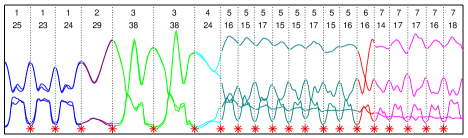
Figure 3.11: Time series corresponding to the recording of the leg positions of an individual performing repetitions of the actions low jumping up and down, high jumping up and down, hopping on the left foot, and hopping on the right foot. The dotted vertical lines give a manual segmentation into 7 basic movements and their repetitions. The numbers in the first row indicate the movement types, whilst the numbers in the second row indicate the durations. The stars indicate the segmentation obtained with the explicit-duration SLGSSM (the movement types were all correctly inferred).

In this section we show that the explicit-duration SLGSSM with across-segment independence and the constraint $\pi_{ii}\neq 0$ can be used to solve the segmentation task discussed in Chapter 1, namely to segment the time series displayed in Figure 3.11 – corresponding to the recording of the leg positions of an individual performing repetitions of the actions low jumping up and down, high jumping up and down, hopping on the left foot, and hopping on the right foot – into the underlying actions and their repetitions.

The time series was manually segmented with the help of an associated video, assuming 7 basic movement types. The manual segmentation is shown in Figure 3.11, where the dotted vertical lines indicate the movement starts, the numbers in the first row indicate the movement types, and the numbers in the second row indicate the durations.

We used the manual segmentation and 7 LGSSMs to learn the parameters representing each movement type. We then performed extended Viterbi with an explicit-duration SLGSSM using the learned parameters and employing a uniform segment-duration distribution, with minimum and maximum durations 15 and 50 for the first 4 types of movement respectively, and 10 and 25 for the second 3 types of movement respectively.

The model correctly inferred all movement types and accurately detected the movement starts, as indicated by the stars in Figure 3.11.

3.6 Approximations

Whilst empowering standard MSMs with stronger modelling capabilities, explicit-duration MSMs can have high computational cost. For simplicity, consider the case of one regime only. The computation of $\alpha^{\sigma_{t}}_{t}=p(\sigma_{t}|v_{1:t})$ and $\gamma^{\sigma_{t}}_{t}=p(\sigma_{t}|v_{1:T})$ has cost ${\cal O}(Td_{\max})$. In models with unobserved variables $h_{1:T}$ related by first-order Markovian dependence, the computation of $\hat{\alpha}^{\sigma_{t}}_{t}=p(h_{t}|\sigma_{t},v_{1:t})$ and $\hat{\gamma}^{\sigma_{t}}_{t}=p(h_{t}|\sigma_{t},v_{1:T})$ has also at best cost ${\cal O}(Td_{\max})$. If $d_{\max}$ is large the cost becomes prohibitive. If $d_{\max}=\infty$, the cost becomes at best ${\cal O}(T^{2})$. Several approximation techniques have been proposed in the literature to address this issue.

A review of approximation methods introduced for extended Viterbi in the explicit-duration HMM is given in Ostendorf et al. (1996). The basic idea is to reduce the space of possible segmentations by constraining the maximization. For example, in the segmental extended Viterbi of §3.4.3, maximization over $d_{t}$ can be constrained to a subset ${\cal D}_{t}$ of the original set $\{d_{\min},\ldots,d_{\max}\}$. The subset ${\cal D}_{t}$ can be chosen in advance with a simpler model or during the decoding.

Pruning methods were also introduced in the changepoint/reset model literature. In changepoint/reset models, dependence from the past is cut at the occurrence of a changepoint. Older approaches employ one regime only, and therefore the occurrence of a changepoint corresponds to the reset of the current dynamics to its initial condition. More recent approaches can employ more than one regime, and therefore the occurrence of a changepoint can also correspond to the reset and change of the current dynamics. Whilst the goal of changepoint models is only to detect abrupt changes in the time series, reset models are also often used as approximations of complex models. Commonly, changepoint/reset models do not impose constraints on the segment duration.

Older approaches to changepoint models fix the number of changepoints a priori. More recent Bayesian approaches define a distribution on the number and positions of changepoints through a segment-duration distribution (Fearnhead, 2006; Fearnhead and Liu, 2007; Adams and MacKay, 2007; Fearnhead and Vasileiou, 2009; Eckley et al., 2011). This is achieved by using either increasing count variables or variables that indicate the time-step of the most recent changepoint prior to time-step $t$ (i.e. $c_{t}=c_{t-1}$ or $c_{t}=t-1$), which provide the same information as increasing count variables.

In reset models, dependence cut is commonly obtained with a variable $c_{t}$ taking value 1 when a changepoint occurs and 2 otherwise (Cemgil et al., 2006; Barber and Cemgil, 2010) (e.g. with $p(c_{t}=2)=\lambda$ and $p(c_{t}=1)=1-\lambda$, which gives a geometric segment-duration distribution – this approach can be seen as a special case of the increasing-count-variable approach). As discussed in §3.5, Bracegirdle and Barber (2011) and Bracegirdle (2013) recently suggested the use of increasing count variables and increasing-decreasing count variables in reset models in order to achieve sequential filtering-smoothing and to approximate inference.

To understand the basic idea of the pruning methods suggested, consider the increasing-count-variable approach with $d_{\max}=\infty$ and the constraint $p(c_{t}>t)=0$ (obtained, e.g., by imposing $\tilde{\lambda}_{1}=1$, see §3.2). From recursion (3.3), we can deduce that $\alpha^{\sigma_{t}}_{t}=0$ implies $\alpha^{s_{t},c_{t}+1}_{t+1}=\ldots=\alpha^{s_{t},c_{t}+T-t}_{T}=0$, i.e. if according to $v_{1:t}$ a segment starting at time-step $t-c_{t}+1$ and generated by $s_{t}$ cannot have duration $\geq c_{t}$, that segment cannot have duration $\geq c_{t}+1$ after incorporating observations $v_{t+1}$, etc. If only ${\cal D}$ elements of $\alpha^{\sigma_{t}}_{t}$ are non-zero, then only ${\cal D}+1$ elements of $\alpha^{s_{t},c_{t+1}}_{t+1}$ are non-zero, and so on. Therefore, we can retain only ${\cal D}$ elements of the count variable by eliminating one element at each time-step, reducing the computational cost from ${\cal O}(T^{2})$ to ${\cal O}(T{\cal D})$. As $\alpha^{\sigma_{t}}_{t}=0$ implies $\gamma^{\sigma_{t}}_{t}=\gamma^{s_{t},c_{t}+1}_{t+1}=\ldots=\gamma^{s_{t},c_{t}+T-t}_{T}=0$ (recursion (3.4)), pruning of $\alpha^{\sigma_{t}}_{t}$ automatically reduces the cost of computing $\gamma^{\sigma_{t}}_{t}$ to ${\cal O}(T{\cal D})$.

A similar reasoning can be made in the count-duration-variable approach with $d_{\max}=\infty$ and the constraint $p(d_{t}>t,c_{t}=1)=0$ (obtained, e.g., by imposing $\tilde{\tilde{\rho}}_{d_{1}d_{1}}=1$, see §3.3), by looking at time-recursive routines (A.7) and (A.9). From routine (A.7), we deduce that $\alpha^{\sigma_{t}}_{t}=0$ implies $\alpha^{s_{t},d_{t},c_{t}-1}_{t+1}=\ldots=\alpha^{s_{t},d_{t},1}_{t+c_{t}-1}=0$ and $\alpha^{s_{t},d_{t}^{\prime},c_{t}^{\prime}}_{t}=0$ if $d_{t}-c_{t}=d_{t}^{\prime}-c_{t}^{\prime}$, i.e. if according to $v_{1:t}$ a segment starting at time-step $t-d_{t}+c_{t}$ and generated by $s_{t}$ cannot have duration $\geq d_{t}-c_{t}+1$, that segment cannot have duration $\geq d_{t}-c_{t}+2$ after incorporating observations $v_{t+1}$, etc. From routine (A.9), we deduce that $\alpha^{\sigma_{t}}_{t}=0$ implies $\gamma^{\sigma_{t}}_{t}=\gamma^{s_{t},d_{t},c_{t}-1}_{t+1}=\ldots=\gamma^{s_{t},d_{t},1}_{t+c_{t}-1}=0$.

For the explicit-duration SLGSSM with across-segment independence, this pruning procedure implies that, instead of LGSSM filtering on $v_{t:T}$ for each $t$ and $s_{t}$ with cost ${\cal O}(T^{2}S)$ and LGSSM smoothing on $v_{t:t+d_{t}-1}$ for each $t$, $d_{t}\in\{1,\ldots,T-t+1\}$ and $s_{t}$ with cost ${\cal O}(T^{3}S)$, only LGSSM filtering on $v_{t:t+{\cal D}-1}$ for each $t$ and $s_{t}$ with cost ${\cal O}(TS{\cal D})$ and LGSSM smoothing on $v_{t:t+d_{t}-1}$ for each $t$ and $d_{t}\in\{1,\ldots,{\cal D}\}$ with cost ${\cal O}(T{\cal D}^{2})$ is required.

Pruning is performed using a resampling idea from Fearnhead and Liu (2007); Liu et al. (1998) in Fearnhead and Vasileiou (2009), and by dropping the element of $\alpha^{\sigma_{t}}_{t}$ with lowest value in Bracegirdle and Barber (2011) and Bracegirdle (2013).

Other approximation techniques based on combining regime variables with and without corresponding explicit-duration variables, on binning the duration distribution and on beam-sampling were proposed in Stanke and Waack (2003), Jiang (2010) and Dewar et al. (2012) respectively.

Chapter 4 Discussion

Explicit-duration Markov switching models (MSMs) enrich the modelling capabilities of standard MSMs with the possibility to define segment-duration distributions of any form, to impose complex dependence between the observations, and to reset the dynamics to initial conditions.

From a generative viewpoint, they differ from standard MSMs as the regime variable $s_{t}$ is either sampled from the transition distribution or set to $s_{t-1}$, depending on the values taken by the explicit-duration variables. This mechanism is achieved through a first-order Markov chain on the combined regime and explicit-duration variables that partitions the time series into segments, with boundaries at those time-steps in which sampling occurs.

The first-order Markov chain can be defined using three fundamentally different encodings for the explicit-duration variables, namely distance to current-segment end with decreasing count variables, distance to current-segment beginning with increasing count variables, or distance to both current-segment beginning and current-segment end with count-duration variables.

Different encoding leads to different possible structures for the conditional distribution of the observations. Information about both segment beginning and segment end allows the most complex structure, namely any conditional distribution within a segment. In this complex case, inference can only be achieved with recursions that operate at a segment level rather than at a single time-step level.

In models that have complex unobserved structure, different encoding gives rise to different computational cost and approximation requirements for inference. As we have seen in §3.5.3, in models containing additional unobserved variables related by first-order Markovian dependence, increasing count variables are overall preferable.

In the literature, explicit-duration MSMs are most commonly called hidden semi-Markov models or segment models and are informally described as extensions of standard MSMs in which, rather than single observations, segments of observations are generated from a sampled regime (Ostendorf et al., 1996; Yu, 2010). They originate from the idea to extend the hidden Markov model by defining a semi-Markov process on the regime variables. The original approach, introduced in Ferguson (1980) and later re-explained in Rabiner (1989), achieves that by introducing duration variables, and by deriving inference recursions that operate at a segment level. This approach is currently the most common approach to explicit-duration modelling.

Although count-duration variables are mentioned in Yu (2010), their use to simplify derivations with respect to the standard approach first appeared in Chiappa and Peters (2010). As we have seen in §3.4.3 and Appendix A.3, computing posterior distributions at time-steps that do not correspond to segment ends with count-duration variables is more immediate than with the standard approach. The benefit is particularly evident when full inference in models that have complex unobserved structure is required, as discussed in §3.5.3.

The decreasing-count-variable approach with independence among observations was introduced in Yu and Kobayashi (2003a) to enable the derivation of computationally less expensive inference routines than the segmental routines. However, as explained in §3.4.3 and already observed in Mitchell et al. (1995) and Murphy (2002), the same improvement can also be reached with recursive computation of the segment-emission distribution in the segmental routines.

Work in the direction of increasing count variables first appeared in Djurić and Chun (2002), but explicit introduction was given in Huang et al. (2006) and Oh et al. (2008).

Appendix A Miscellaneous

A.1 EM in the Switching Autoregressive Model

Consider the switching autoregressive model (2.2) with $\tilde{v}_{t}=[v_{t-k}\ldots v_{t-1}]^{\textsf{T}}$, where the symbol ${}^{\textsf{T}}$ indicates the transpose operator, and $a^{s_{t}}=[a^{s_{t}}_{1}\ldots a^{s_{t}}_{k}]$. The expectation of the complete data log-likelihood is given by (omitting the first $k$ observations)

$$\hskip-1.42271pt\sum_{t=k+1}^{T}\!\!\langle\log p(v_{t}|s_{t},v_{t-k:t-1})\rangle_{\gamma^{s_{t}}_{t}}\!+\!\langle\log p(s_{1})\rangle_{\gamma^{s_{1}}_{1}}\!+\!\sum_{t=2}^{T}\langle\log p(s_{t}|s_{t-1})\rangle_{\tilde{\gamma}^{s_{t-1:t}}_{t}}\!=\!$$

$$\!-\!\frac{1}{2}\sum_{t}\langle\log(\sigma^{s_{t}})^{2}\!+\!\frac{(v_{t}\!-\!a^{s_{t}}\tilde{v}_{t})^{2}}{(\sigma^{s_{t}})^{2}}\rangle_{\gamma^{s_{t}}_{t}}\!+\!\langle\log\tilde{\pi}_{s_{1}}\rangle_{\gamma^{s_{1}}_{1}}\!+\!\sum_{t}\langle\log\pi_{s_{t}s_{t-1}}\rangle_{\tilde{\gamma}^{s_{t-1:t}}_{t}},$$

where (see Equation (2.5))

$$\tilde{\gamma}^{s_{t-1:t}}_{t} =p(s_{t-1:t}|v_{1:T})=\frac{\pi_{s_{t}s_{t-1}}\alpha^{s_{t-1}}_{t-1}}{\sum_{\tilde{s}_{t-1}}\pi_{s_{t}\tilde{s}_{t-1}}\alpha^{\tilde{s}_{t-1}}_{t-1}}\gamma^{s_{t}}_{t},$$

giving updates

$$a^{s_{t}}=\sum_{t}\gamma^{s_{t}}_{t}v_{t}\tilde{v}_{t}^{\textsf{T}}\big{(}\sum_{t}\gamma^{s_{t}}_{t}\tilde{v}_{t}\tilde{v}_{t}^{\textsf{T}}\big{)}^{-1},\hskip 8.5359pt(\sigma^{s_{t}})^{2}=\frac{\sum_{t}\gamma^{s_{t}}_{t}(v_{t}-a^{s_{t}}\tilde{v}_{t})^{2}}{\sum_{t}\gamma^{s_{t}}_{t}},$$

$$\tilde{\pi}_{s_{1}}=\gamma^{s_{1}}_{1},\hskip 8.5359pt\pi_{s_{t}s_{t-1}}=\frac{\sum_{t=2}^{T}\tilde{\gamma}^{s_{t-1:t}}_{t}}{\sum_{t=2}^{T}\sum_{\tilde{s}_{t}}\tilde{\gamma}^{s_{t-1},\tilde{s}_{t}}_{t}}.$$

A.2 HMM as a Decreasing-Count-Variable MSM

The HMM with initial-regime distribution $\tilde{\hat{\pi}}$ and transition distribution $\hat{\pi}$ has the same joint distribution $p(s_{1:T},v_{1:T})$ of a decreasing-count-variable MSM with $d_{\min}=1,d_{\max}=\infty$, and with

$$\tilde{\pi}_{s_{1}}=\tilde{\hat{\pi}}_{s_{1}}\,,\hskip 8.5359pt\pi_{s_{t+1}s_{t}}=\begin{cases}\frac{\hat{\pi}_{s_{t+1}s_{t}}}{1-\hat{\pi}_{s_{t}s_{t}}}&\textrm{if }s_{t+1}\!\neq\!s_{t}\\ 0&\textrm{if }s_{t+1}\!=\!s_{t}\,,\end{cases}$$

$$\tilde{\rho}_{\sigma_{1}}=\hat{\pi}^{c_{1}-1}_{s_{1}s_{1}}(1-\hat{\pi}_{s_{1}s_{1}})\,,\hskip 8.5359pt\rho_{\sigma_{t}}=\hat{\pi}^{c_{t}-1}_{s_{t}s_{t}}(1-\hat{\pi}_{s_{t}s_{t}}).$$

This can be demonstrated by showing that

$$\sum_{c_{1:T}}p(s_{1})p(c_{1}|s_{1})\prod_{t=2}^{T}p(s_{t}|\sigma_{t-1})p(c_{t}|s_{t},c_{t-1})=\tilde{\hat{\pi}}_{s_{1}}\prod_{t=2}^{T}\hat{\pi}_{s_{t}s_{t-1}}.$$ (A.1)

Since $\pi_{s_{t}s_{t}}=0$, $s_{1:T}$ determine the values of the count variables at all time-steps with exception of the last segment. Let’s consider the case of two or more regime changes (the other cases can be demonstrated similarly). Suppose that two consecutive regime changes occur at time-steps $\tau+1>1$ and $\tau+d+1\leq T$, i.e. $s_{\tau}\neq s_{\tau+1}=\cdots=s_{\tau+d}\neq s_{\tau+d+1}$. Then $c_{\tau}=1,c_{\tau+1}=d,\ldots,c_{\tau+d-1}=2,c_{\tau+d}=1$, and therefore

$$\hskip-2.84544pt\prod_{t=\tau+1}^{\tau+d}\!\!\!p(s_{t}|\sigma_{t-1})p(c_{t}|s_{t},c_{t-1}) =p(s_{\tau+1}|s_{\tau},c_{\tau}\!=\!1)p(c_{\tau+1}|s_{\tau+1},c_{\tau}\!=\!1)$$

$$=(1\!-\!\hat{\pi}_{s_{\tau+1}s_{\tau+1}})\pi_{s_{\tau+1}s_{\tau}}\prod_{t=\tau+2}^{\tau+d}\!\!\!\hat{\pi}_{s_{t}s_{t-1}}$$

$$=\frac{1\!-\!\hat{\pi}_{s_{\tau+1}s_{\tau+1}}\!=\!n_{\tau+1}}{1\!-\!\hat{\pi}_{s_{\tau}s_{\tau}}\!=\!n_{\tau}}\prod_{t=\tau+1}^{\tau+d}\hat{\pi}_{s_{t}s_{t-1}}.$$ (A.2)

There are two possible scenarios for the change of regime after time-step $\tau+d+1$, namely it occurs

• At time-step $T$ or before, i.e. $s_{\tau+d+1}=\cdots=s_{\tau+d^{\prime}}\neq s_{\tau+d^{\prime}+1}$ with $\tau+d^{\prime}<T$, giving

  $$\prod_{t=\tau+d+1}^{\tau+d^{\prime}}\!\!\!p(s_{t}|\sigma_{t-1})p(c_{t}|s_{t},c_{t-1}) \!=\!\frac{1\!-\!\hat{\pi}_{s_{\tau+d+1}s_{\tau+d+1}}}{1\!-\!\hat{\pi}_{s_{\tau+d}s_{\tau+d}}\!=\!n_{\tau+1}}\prod_{t=\tau+d+1}^{\tau+d^{\prime}}\!\!\!\!\hat{\pi}_{s_{t}s_{t-1}}.$$

• After time-step $T$, i.e. $s_{\tau+d+1}=\cdots=s_{T}$, giving

  $$\sum_{c_{\tau+d+1:T}}\prod_{t=\tau+d+1}^{T} p(s_{t}|\sigma_{t-1})p(c_{t}|s_{t},c_{t-1})=\pi_{s_{\tau+d+1}s_{\tau+d}}$$

  $$\times\underbrace{(1\!-\!\hat{\pi}_{s_{\tau+d+1}s_{\tau+d+1}})\hskip-5.69046pt\sum_{c_{\tau+d+1}=T-\tau-d}^{\infty}\hskip-5.69046pt\hat{\pi}_{s_{\tau+d+1}s_{\tau+d+1}}^{c_{\tau+d+1}-1}}_{\hat{\pi}_{s_{\tau+d+1}s_{\tau+d+1}}^{T-\tau-d-1}}$$

  $$=\frac{1}{1\!-\!\hat{\pi}_{s_{\tau+d}s_{\tau+d}}\!=\!n_{\tau+1}}\prod_{t=\tau+d+1}^{T}\hskip-2.84544pt\hat{\pi}_{s_{t}s_{t-1}}.$$

Analogously, there are two possible scenarios for the change of regime before time-step $\tau+1$, namely it occurs

• After time-step 1, i.e. $s_{\tau-d^{\prime}}\neq s_{\tau-d^{\prime}+1}=\cdots=s_{\tau}$ with $\tau-d^{\prime}+1>1$, giving

  $$\prod_{t=\tau-d^{\prime}+1}^{\tau}\hskip-11.38092ptp(s_{t}|\sigma_{t-1})p(c_{t}|s_{t},c_{t-1}) \!=\!\frac{1\!-\!\hat{\pi}_{s_{\tau-d^{\prime}+1}s_{\tau-d^{\prime}+1}}\!\!=\!n_{\tau}}{1\!-\!\hat{\pi}_{s_{\tau-d^{\prime}}s_{\tau-d^{\prime}}}}\hskip-12.80365pt\prod_{t=\tau-d^{\prime}+1}^{\tau}\hskip-11.38092pt\hat{\pi}_{s_{t}s_{t-1}}.$$

• At time-step 1 or before, giving

  $$\prod_{t=1}^{\tau}p(s_{t}|\sigma_{t-1})p(c_{t}|s_{t},c_{t-1}) =(1\!-\!\hat{\pi}_{s_{1}s_{1}}\!=\!n_{\tau})\tilde{\hat{\pi}}_{s_{1}}\prod_{t=2}^{\tau}\hat{\pi}_{s_{t}s_{t-1}}.$$

Therefore, in Equation (A.1), $n_{\tau+1}$ of Equation (A.2) cancels with $n_{\tau+1}$ in the following regime, whilst $n_{\tau}$ cancels with $n_{\tau}$ in the preceding regime.

Notice that, to use the model, conditioning on the event $c_{T}=1$ would be required and the equivalence would not longer hold.

The recursion for $p(s_{t},v_{1:t})$ using recursion (3.1) reduces to the HMM recursion for $p(s_{t},v_{1:t})$ (see recursion (2.3)). Indeed

$$p(s_{t}, v_{1:t})=\sum_{c_{t}=1}^{\infty}p(\sigma_{t},v_{1:t})=\sum_{c_{t}=1}^{\infty}\hat{\alpha}^{\sigma_{t}}_{t}$$

$$=p(v_{t}|s_{t})\sum_{c_{t}=1}^{\infty}\bigg{\{}\hat{\alpha}^{s_{t},c_{t}+1}_{t-1}+\rho_{\sigma_{t}}\sum_{s_{t-1}\neq s_{t}}\pi_{s_{t}s_{t-1}}\hat{\alpha}^{s_{t-1},1}_{t-1}\bigg{\}}$$

$$=p(v_{t}|s_{t})\bigg{\{}\sum_{c_{t}=1}^{\infty}\hat{\pi}_{s_{t}s_{t}}\hat{\alpha}^{\sigma_{t}}_{t-1}\!+\!\hskip-5.69046pt\sum_{s_{t-1}\neq s_{t}}\hskip-7.11317pt\pi_{s_{t}s_{t-1}}\hskip-15.6491pt\underbrace{(1\!-\!\hat{\pi}_{s_{t}s_{t}})\sum_{c_{t}=1}^{\infty}\hat{\pi}^{c_{t}-1}_{s_{t}s_{t}}}_{(1\!-\!\hat{\pi}_{s_{t-1}s_{t-1}})\sum_{c_{t}=1}^{\infty}\hat{\pi}^{c_{t}-1}_{s_{t-1}s_{t-1}}}\hskip-15.6491pt\hat{\alpha}^{s_{t-1},1}_{t-1}\bigg{\}}$$

$$=p(v_{t}|s_{t})\sum_{s_{t-1}}\hat{\pi}_{s_{t}s_{t-1}}\sum_{c_{t-1}=1}^{\infty}\hat{\alpha}^{\sigma_{t-1}}_{t-1},$$

where $\hat{\alpha}^{s_{t},c_{t}}_{t}=\hat{\pi}_{s_{t}s_{t}}\hat{\alpha}^{s_{t},c_{t}-1}_{t}$ for $c_{t}>1$, and therefore $\hat{\alpha}^{\sigma_{t}}_{t}=\hat{\pi}_{s_{t}s_{t}}^{c_{t}-1}\hat{\alpha}^{s_{t},1}_{t}$, can be proven by induction. The proof is trivial for $t=1$. Suppose that the result holds for $t-1$, then it holds for $t$ as

$$\hat{\alpha}^{\sigma_{t}}_{t} =p(v_{t}|s_{t})\bigg{\{}\hat{\alpha}^{s_{t},c_{t}+1}_{t-1}+\rho_{\sigma_{t}}\sum_{s_{t-1}\neq s_{t}}\pi_{s_{t}s_{t-1}}\hat{\alpha}^{s_{t-1},1}_{t-1}\bigg{\}}$$

$$=p(v_{t}|s_{t})\bigg{\{}\hat{\pi}_{s_{t}s_{t}}\hat{\alpha}^{s_{t},c_{t}}_{t-1}+\hat{\pi}_{s_{t}s_{t}}\hat{\pi}_{s_{t}s_{t}}^{c_{t}-1-1}(1-\hat{\pi}_{s_{t}s_{t}})\hskip-2.84544pt\sum_{s_{t-1}\neq s_{t}}\hskip-2.84544pt\pi_{s_{t}s_{t-1}}\hat{\alpha}^{s_{t-1},1}_{t-1}\bigg{\}}$$

$$=\hat{\pi}_{s_{t}s_{t}}\hat{\alpha}^{s_{t},c_{t}-1}_{t}.$$

The HMM recursion for $p(v_{t+1:T}|s_{t},v_{t-k+1:t})$ (see recursion (2.4)) cannot be obtained.

A.3 Relation between EM in §3.4.3 and in Rabiner (1989)

In the explicit-duration HMM of Rabiner (1989), $\alpha_{t}(s_{t})$ (Equation (65)) corresponds to the sum over $d_{t}$ of $\bar{\alpha}^{\sigma^{1}_{t}}=p(s_{t},d_{t},c_{t}=1,v_{1:t})$, whilst $\beta_{t}(s_{t})$ (Equation (72)) is equivalent to $\beta^{s_{t},1}_{t}=p(v_{t+1:T}|s_{t},c_{t}=1)$. Rabiner (1989) additionally defines the joint probability of observations up to time $t$ and change to regime $s_{t+1}$ at time-step $t+1$, $\alpha^{*}_{t}(s_{t+1})$ (Equation (71)), and the probability of observations from time $t+1$ given change to regime $s_{t+1}$, $\beta^{*}_{t}(s_{t+1})$ (Equation (73)).

The update for the segment-duration distribution is given by (Equation (81))

$$\bar{\rho}_{s_{t}}(d_{t})=\frac{\sum_{t=1}^{T}\alpha^{*}_{t}(s_{t})\rho_{s_{t}}(d_{t})\beta_{t+d_{t}}(s_{t})\prod_{s=t+1}^{t+d_{t}}b_{s_{t}}(O_{s})}{\sum_{d_{t}=1}^{D}\sum_{t=1}^{T}\alpha^{*}_{t}(s_{t})\rho_{s_{t}}(d_{t})\beta_{t+d_{t}}(s_{t})\prod_{s=t+1}^{t+d_{t}}b_{s_{t}}(O_{s})}.$$

From the relation between $\alpha_{t}(s_{t})$ and $\alpha^{*}_{t}(s_{t})$ (Equation (75))

$$\alpha_{t}(s_{t})=\sum_{d_{t}}\alpha^{*}_{t-d_{t}}(s_{t})\rho_{s_{t}}(d_{t})\prod_{s=t-d_{t}+1}^{t}b_{s_{t}}(O_{s}),$$

we obtain $\alpha^{*}_{t}(s_{t})\rho_{s_{t}}(d_{t})\prod_{s=t+1}^{t+d_{t}}b_{s_{t}}(O_{s})=\bar{\alpha}^{s_{t},d_{t},1}_{t+d_{t}}$, which gives equivalence with update (3.10).

The update for the transition distribution is given by (Equation (79))

$$\bar{a}_{s_{t-1}s_{t}}=\frac{\sum_{t=2}^{T}\alpha_{t-1}(s_{t-1})a_{s_{t-1}s_{t}}\beta^{*}_{t-1}(s_{t})}{\sum_{j=1}^{N}\sum_{t=2}^{T}\alpha_{t-1}(s_{t-1})a_{s_{t-1}s_{t}}\beta^{*}_{t-1}(s_{t})}.$$

Equation (3.12) can be expressed in terms of $\bar{\alpha}^{\sigma^{1}_{t-1}}_{t-1}$ and $\beta^{s_{t},1}_{t+d_{t}-1}$ as

$$p(s_{t-1},c_{t-1}\!=\!1,s_{t}|v_{1:T}) =\frac{\pi_{s_{t}s_{t-1}}\sum_{d_{t-1}}\alpha^{\sigma^{1}_{t-1}}_{t-1}}{\sum_{\tilde{s}_{t-1}}\pi_{s_{t}\tilde{s}_{t-1}}\sum_{\tilde{d}_{t-1}}\alpha^{\tilde{\sigma}^{1}_{t-1}}_{t-1}}\sum_{d_{t}}\gamma^{s_{t},d_{t},1}_{t+d_{t}-1}$$

$$\propto\pi_{s_{t}s_{t-1}}\sum_{d_{t-1}}\bar{\alpha}^{\sigma^{1}_{t-1}}_{t-1}\sum_{d_{t}}\beta^{s_{t},1}_{t+d_{t}-1}\rho_{s_{t}d_{t}}p(v_{t:t+d_{t}-1}).$$

From the relation between $\beta^{*}_{t}(s_{t})$ and $\beta_{t}(s_{t})$ (Equation (77)), we obtain

$$\beta^{*}_{t-1}(s_{t})=\sum_{d_{t}}\hat{\beta}_{t+d_{t}-1}(s_{t})\rho_{s_{t}}(d_{t})\prod_{s=t}^{t+d_{t}-1}b_{s_{t}}(O_{s}),$$

and therefore $p(s_{t-1},c_{t-1}\!=\!1,s_{t}|v_{1:T})\propto\pi_{s_{t}s_{t-1}}\alpha_{t-1}(s_{t-1})\beta^{*}_{t-1}(s_{t})$, which gives equivalence with update (3.11).

The smoothed distribution $p(s_{t}|v_{1:T})$ is computed as $p(s_{t}|v_{1:T})\propto\sum_{\tau<t}\alpha^{*}_{\tau}(s_{t})\beta^{*}_{\tau}(s_{t})-\beta_{\tau}(s_{t})\alpha_{\tau}(s_{t})$ (Equation (80)), i.e. by summing over the set of segments passing through time-step $t$, which is obtained by subtracting all segments ending before time-step $t$ from all segments starting at time-step $t$ or before. In Equation (3.8), we instead obtain this set as the set of segments that start at time-step $t$ or before and end at time-step $t$ or after.

A.4 Robot Localization with the SLGSSM

In this section, we describe in detail the robot localization problem discussed §1 and in §3.5. Consider a two-wheeled robot moving at constant velocity in the two-dimensional plane. At each time-step, the robot undertakes one of the following three types of movement:

• Straight movement: Move both wheels forward by the same distance $k$ ($DR=DL=k$, where $DR$ and $DL$ indicate the distance traveled by the right and left wheel respectively).

• Right-wheel rotation: Move the right wheel forward and keep the left wheel fixed ($DR=2k,DL=0$).

• Left-wheel rotation: Move the left wheel forward and keep the right wheel fixed ($DR=0,DL=2k$).

Due to external forces affecting the motion, such as wheel slippage, the movements effectively performed by the robot differ slightly from the intended ones. The location of the robot at time-step $t$ is defined by a triplet $(x_{t},y_{t},\phi_{t})$, where $x_{t}$ and $y_{t}$ represent the position of the midpoint of the wheel axle, whilst $\phi_{t}$ represents the orientation of the robot (angle formed by the perpendicular to the wheel axle and the horizontal axis). The dynamics of the robot is given by (Wang, 1990)

$$x_{t}=x_{t-1}+r\Delta D\cos(\phi_{t-1}+\Delta\phi/2)+\eta^{x}_{t},$$

$$y_{t}=y_{t-1}+r\Delta D\sin(\phi_{t-1}+\Delta\phi/2)+\eta^{y}_{t},$$

$$\phi_{t}=\phi_{t-1}+\Delta\phi+\eta^{\phi}_{t},$$ (A.3)

with $\Delta D=(DR+DL)/2$, $\Delta\phi=(DR-DL)/L$ (where $L$ is the width of the mower), and with $r=1$, $r=\sin(\Delta\phi/2)/(\Delta\phi/2)$ for straight and rotation movements respectively. In Equation (A.4), $\eta^{x}_{t},\eta^{y}_{t}$ and $\eta^{\phi}_{t}$ are Gaussian noise terms that account for the external forces responsible for the deviations from the intended movements.

Suppose that, due to errors in the measurement system, only noisy measurements of the positions can be obtained. The goal is to estimate, at each time-step $t$, the actual robot position from the set of measurements up to time-step $t$ (on-line localization) and from all measurements (off-line localization). We can compactly write Equation (A.4) and the observation process as

$$h_{1}\!=\![x_{1}\hskip 2.84544pty_{1}\hskip 2.84544pt\phi_{1}]^{\textsf{T}}\!\sim\!{\cal N}(h_{1};\mu,\Sigma),$$

$$h_{t}\!=\!f^{s_{t}}(h_{t-1})+\eta^{h}_{t},\hskip 2.84544pth_{t-1}\!=\![x_{t}\hskip 2.84544pty_{t}\hskip 2.84544pt\phi_{t}]^{\textsf{T}},\hskip 2.84544pt\eta^{h}_{t}\!=\![\eta^{x}_{t}\hskip 2.84544pt\eta^{y}_{t}\hskip 2.84544pt\eta^{\phi}_{t}]^{\textsf{T}}\!\sim\!{\cal N}(\eta^{h}_{t};0,\Sigma_{H}),$$

$$v_{t}\!=\!Bh_{t}+\eta^{v}_{t},\hskip 8.5359ptB=\left[\begin{array}[]{ccc}1&0&0\\ 0&1&0\\ \end{array}\right],\hskip 8.5359pt\eta^{v}_{t}\sim{\cal N}(\eta^{v}_{t};0,\Sigma_{V}),$$ (A.6)

where $s_{t}\in\{1,2,3\}$ indicates the type of movement undertaken by the robot, and $f^{s_{t}}$ is the corresponding nonlinear function. We have therefore formulated the model as a SLGSSM with the only difference that the hidden dynamics evolves nonlinearly. We can deal with that with an unscented approximation similar to one proposed in Särkkä (2008) for the LGSSM, which enables us to use similar inference routines to the linear case.

A.5 Count-Duration-Variable SLGSSM

In this section, we provide time-recursive inference routines for the explicit-duration SLGSSM that uses count-duration variables.

Filtering

The recursion for $\alpha^{\sigma_{t}}_{t}=p(\sigma_{t}|v_{1:t})$ is given by

$$\alpha^{\sigma_{t}}_{t} =\frac{\sum_{\sigma_{t-1}}p(v_{t},\sigma_{t-1:t}|v_{1:t-1})}{\sum_{\tilde{\sigma}_{t-1:t}}p(v_{t},\tilde{\sigma}_{t-1:t}|v_{1:t-1})}$$

$$\propto\sum_{\sigma_{t-1}}p(v_{t}|\sigma_{t-1},s_{t},\cancel{d_{t},c_{t}},v_{1:t-1})p(\sigma_{t}|\sigma_{t-1},\cancel{v_{1:t-1}})p(\sigma_{t-1}|v_{1:t-1})$$

$$=\delta_{\begin{subarray}{l}c_{t}<d_{t}\\ s_{t-1}=s_{t}\\ d_{t-1}=d_{t}\\ c_{t-1}=c_{t}+1\end{subarray}}\hskip-8.5359pte^{\sigma_{t-1},s_{t}}_{t}\alpha^{\sigma_{t-1}}_{t-1}+\delta_{\begin{subarray}{l}c_{t}=d_{t}\\ c_{t-1}=1\end{subarray}}\hskip 0.0pt\rho_{s_{t}d_{t}}\sum_{s_{t-1}}\pi_{s_{t}s_{t-1}}e^{\sigma_{t-1},s_{t}}_{t}\sum_{d_{t-1}}\alpha^{\sigma_{t-1}}_{t-1},$$

where $e^{\sigma_{t-1},s_{t}}_{t}=p(v_{t}|\sigma_{t-1},s_{t},v_{1:t-1})$. With pre-summation over $d_{t-1}$, this recursion has computational cost ${\cal O}(TS^{2}d^{2}_{\max})$.

However, notice that $\alpha^{\sigma_{t}}_{t}$ and $\alpha^{\sigma_{t}^{\prime}}_{t}$ for which $d_{t}-c_{t}=d^{\prime}_{t}-c^{\prime}_{t}$ differ only in $\rho_{s_{t}d_{t}}$ and $\rho_{s^{\prime}_{t}d^{\prime}_{t}}$. As $d_{t}-c_{t}$ ranges from 0 to $d_{\max}-1$, we can define a variable $\tilde{c}_{t}\in\{1,\ldots,d_{\max}\}$ and form a recursion over $\tilde{\alpha}^{\tilde{c}_{t}}_{t}$ such that $\alpha^{\sigma_{t}}_{t}=\rho_{s_{t}d_{t}}\tilde{\alpha}^{s_{t},d_{t}-c_{t}}_{t}$. This approach reduces the cost to ${\cal O}(TS^{2}d_{\max})$ (a similar approach was introduced in Jiang (2010)).

Notice that $\alpha^{\sigma_{t}}_{t}=0$ implies $\alpha^{s_{t},d_{t},c_{t}-1}_{t+1}=\ldots=\alpha^{s_{t},d_{t},1}_{t+c_{t}-1}=0$ and $\alpha^{\sigma_{t}^{\prime}}_{t}=0$ if $d_{t}-c_{t}=d_{t}^{\prime}-c_{t}^{\prime}$, i.e. if according to $v_{1:t}$ a segment starting at time-step $t-d_{t}+c_{t}$ and generated by $s_{t}$ cannot have duration $\geq d_{t}-c_{t}+1$, that segment cannot have duration $\geq d_{t}-c_{t}+2$ after incorporating observations $v_{t+1}$, etc.

The recursion for $\hat{\alpha}^{\sigma_{t}}_{t}=p(h_{t}|\sigma_{t},v_{1:t})$ is given by

$$\hat{\alpha}^{\sigma_{t}}_{t} =\sum_{\sigma_{t-1}}p(h_{t}|\sigma_{t-1},s_{t},\cancel{d_{t},c_{t}},v_{1:t})p(\sigma_{t-1}|\sigma_{t},v_{1:t})$$

$$=\Bigg{\{}\delta_{\begin{subarray}{l}c_{t}<d_{t}\\ s_{t-1}=s_{t}\\ d_{t-1}=d_{t}\\ c_{t-1}=c_{t}+1\end{subarray}}\hskip-11.38092pt+\delta_{\begin{subarray}{l}c_{t}=d_{t}\\ c_{t-1}=1\end{subarray}}\frac{\sum_{\begin{subarray}{c}s_{t-1}\\ d_{t-1}\end{subarray}}p(v_{t},\sigma_{t-1:t}|v_{1:t-1})}{\sum_{\tilde{\sigma}_{t-1}}p(v_{t},\tilde{\sigma}_{t-1:t}|v_{1:t-1})}\Bigg{\}}p(h_{t}|\sigma_{t-1},s_{t},v_{1:t}),$$

where we have used $p(\sigma_{t-1}=(s_{t},d_{t},c_{t}+1)|s_{t},d_{t},c_{t}<d_{t})=1$. Therefore, $\hat{\alpha}^{\sigma_{t}}_{t}$ is a Gaussian mixture with a complex number of components. Gaussian collapsing of $\hat{\alpha}^{s_{t},d_{t},c_{t}=d_{t}}_{t}$ reduces the cost to ${\cal O}(TS^{2}d^{2}_{\max})$.

Across-segment independence.

The recursion for $\alpha^{\sigma_{t}}_{t}$ becomes

$$\alpha^{\sigma_{t}}_{t} \propto\sum_{\sigma_{t-1}}p(v_{t}|\sigma_{t-1},s_{t},{\color[rgb]{0.4,0,0}{c_{t},d_{t}}},v_{1:t-1})p(\sigma_{t}|\sigma_{t-1},\cancel{v_{1:t-1}})p(\sigma_{t-1}|v_{1:t-1})$$

$$=\delta_{\begin{subarray}{l}c_{t}<d_{t}\\ s_{t-1}=s_{t}\\ d_{t-1}=d_{t}\\ c_{t-1}=c_{t}+1\end{subarray}}p(v_{t}|\sigma_{t-1:t},v_{1:t-1})\alpha^{\sigma_{t-1}}_{t-1}$$

$$+\delta_{\begin{subarray}{l}c_{t}=d_{t}\\ c_{t-1}=1\end{subarray}}p(v_{t}|{\color[rgb]{0.4,0,0}\cancel{\sigma_{t-1}}},\sigma_{t},{\color[rgb]{0.4,0,0}\cancel{v_{1:t-1}}})\rho_{s_{t}d_{t}}\sum_{s_{t-1}}\pi_{s_{t}s_{t-1}}\sum_{d_{t-1}}\alpha^{\sigma_{t-1}}_{t-1},$$ (A.7)

where $p(v_{t}|s_{t},d_{t},c_{t}=d_{t})={\cal N}(v_{t};B^{s_{t}}\mu^{s_{t}},B^{s_{t}}\Sigma^{s_{t}}(B^{s_{t}})^{\textsf{T}}+\Sigma^{s_{t}}_{V})$. As in the case of across-segment dependence, the computational cost can be reduced to ${\cal O}(TS^{2}d_{\max})$.

The recursion for $\hat{\alpha}^{\sigma_{t}}_{t}=p(h_{t}|\sigma_{t},v_{1:t})$ becomes

$$\hat{\alpha}^{\sigma_{t}}_{t} =\sum_{\sigma_{t-1}}p(h_{t}|\sigma_{t-1},s_{t},{\color[rgb]{0.4,0,0}d_{t},c_{t}},v_{1:t})p(\sigma_{t-1}|\sigma_{t},v_{1:t})$$

$$=\delta_{\begin{subarray}{l}c_{t}<d_{t}\\ s_{t-1}=s_{t}\\ d_{t-1}=d_{t}\\ c_{t-1}=c_{t}+1\end{subarray}}p(h_{t}|\sigma_{t-1:t},v_{1:t})$$

$$+\delta_{\begin{subarray}{l}c_{t}=d_{t}\\ c_{t-1}=1\end{subarray}}\cancel{\sum_{\begin{subarray}{c}s_{t-1}\\ d_{t-1}\end{subarray}}}p(h_{t}|{\color[rgb]{0.4,0,0}\cancel{\sigma_{t-1}}},\sigma_{t},{\color[rgb]{0.4,0,0}\cancel{v_{1:t-1}}},v_{t})\cancel{p(\sigma_{t-1}|\sigma_{t},v_{1:t})},$$ (A.8)

where $p(h_{t}|s_{t},c_{t},d_{t}=c_{t},v_{t})$ is Gaussian with mean and covariance as in Equation (3.19). Therefore $\hat{\alpha}^{\sigma_{t}}_{t}$ is Gaussian. Naive computation of this recursion has cost ${\cal O}(TSd^{2}_{\max})$. However, as $\hat{\alpha}^{\sigma_{t}}_{t}$ varies only with the difference $d_{t}-c_{t}$ for which the segment starts at a different time-step, rather than with single values of $d_{t}$ and $c_{t}$, the cost can be reduced to ${\cal O}(TSd_{\max})$. This recursion essentially performs filtering in a LGSSM on segment $v_{t:t+d_{\max}-1}$ for each $t$ and $s_{t}$, in agreement with the explanation in §3.5.3, and as recursion (3.26).

Smoothing

The recursion for $\gamma^{\sigma_{t}}_{t}=p(\sigma_{t}|v_{1:T})$ is given by

$$\gamma^{\sigma_{t}}_{t} =\delta_{\begin{subarray}{l}c_{t}>1\end{subarray}}\gamma^{s_{t},d_{t},c_{t}-1}_{t+1}+\delta_{\begin{subarray}{l}c_{t}=1\\ c_{t+1}=d_{t+1}\end{subarray}}\sum_{s_{t+1}}\underbrace{p(\sigma_{t}|\sigma_{t+1},v_{1:T})}_{\approx p(\sigma_{t}|h_{t+1}=\hat{h}_{t+1}^{T,\sigma_{t+1}},\sigma_{t+1},v_{1:t})}\gamma^{\sigma_{t+1}}_{t+1},$$

where we have used $p(\sigma_{t}=(s_{t+1},d_{t+1},c_{t+1}+1)|s_{t+1},d_{t+1},c_{t+1}<d_{t+1},v_{1:T})=1$.

The recursion for $\hat{\gamma}^{\sigma_{t}}_{t}$ is given by

$$\hat{\gamma}^{\sigma_{t}}_{t} =\sum_{\sigma_{t+1}}p(h_{t}|\sigma_{t:t+1},v_{1:T})p(\sigma_{t+1}|\sigma_{t},v_{1:T})$$

$$=\Bigg{\{}\delta_{\begin{subarray}{l}c_{t}>1\\ s_{t+1}=s_{t}\\ d_{t+1}=d_{t}\\ c_{t+1}=c_{t}-1\end{subarray}}\hskip-17.07182pt+\delta_{\begin{subarray}{l}c_{t}=1\\ c_{t+1}=d_{t+1}\end{subarray}}\sum_{\begin{subarray}{c}s_{t+1}\\ d_{t+1}\end{subarray}}p(\sigma_{t+1}|\sigma_{t},v_{1:T})\Bigg{\}}p(h_{t}|\sigma_{t:t+1},v_{1:T}),$$

where we have used $p(\sigma_{t+1}=(s_{t},d_{t},c_{t}-1)|s_{t},d_{t},c_{t}>1)=1$.

Notice that the approximation $p(h_{t+1}|\sigma_{t:t+1},v_{1:T})\approx\hat{\gamma}^{\sigma_{t+1}}_{t+1}$ in the computation of $p(h_{t}|\sigma_{t:t+1},v_{1:T})$ (see Equation (3.22)) becomes exact for $c_{t+1}<d_{t+1}$. Indeed $p(h_{t+1}|\sigma_{t},\sigma_{t+1}=(s_{t},d_{t},c_{t}-1),v_{1:T})=p(h_{t+1}|\sigma_{t+1}=(s_{t},d_{t},c_{t}-1),v_{1:T})$ follows from the fact that $d_{t+1}=d_{t}\geq c_{t}>c_{t}-1=c_{t+1}$ and therefore $c_{t}$ must be equal to $c_{t+1}+1$. Therefore $\hat{\gamma}^{\sigma_{t}}_{t}$ is a Gaussian mixture with a complex number of components. Gaussian collapsing of $\hat{\gamma}^{s_{t},c_{t}=1,d_{t}}_{t}$ reduces the cost to ${\cal O}(TS^{2}d^{2}_{\max})$.

Across-segment independence.

From Equations (3.7) and (3.9), we deduce that a time-recursive approach to computing $\gamma^{\sigma_{t}}_{t}=p(\sigma_{t}|v_{1:T})$ is given by

$$\gamma^{\sigma_{t}}_{t}=\delta_{\begin{subarray}{l}c_{t}>1\end{subarray}}\gamma^{s_{t},d_{t},c_{t}-1}_{t+1}+\delta_{\begin{subarray}{l}c_{t}=1\\ c_{t+1}=d_{t+1}\end{subarray}}\sum_{s_{t+1}}p(\sigma_{t}|\sigma_{t+1},v_{1:t},{\color[rgb]{0.4,0,0}\cancel{v_{t+1:T}}})\gamma^{\sigma_{t+1}}_{t+1}\hskip-2.84544pt$$ (A.9)

$$=\delta_{\begin{subarray}{l}c_{t}>1\end{subarray}}\gamma^{s_{t},d_{t},c_{t}-1}_{t+1}+\delta_{\begin{subarray}{l}c_{t}=1\end{subarray}}\alpha^{\sigma^{1}_{t}}_{t}\sum_{s_{t+1}}\frac{\pi_{s_{t+1}s_{t}}}{\sum_{\tilde{s}_{t}}\pi_{s_{t+1}\tilde{s}_{t}}\sum_{\tilde{d}_{t}}\alpha^{\tilde{\sigma}^{1}_{t}}_{t}}\sum_{d_{t+1}}\gamma^{s_{t+1},d_{t+1},d_{t+1}}_{t+1}.$$

This recursion has cost ${\cal O}(TSd^{2}_{\max})$. Notice that $\alpha^{\sigma_{t}}_{t}=0$ implies $\gamma^{\sigma_{t}}_{t}=\gamma^{s_{t},d_{t},c_{t}-1}_{t+1}=\ldots=\gamma^{s_{t},d_{t},1}_{t+c_{t}-1}=0$.

The recursion for $\hat{\gamma}^{\sigma_{t}}_{t}$ becomes

$$\hat{\gamma}^{\sigma_{t}}_{t} =\delta_{\begin{subarray}{l}c_{t}>1\\ s_{t+1}=s_{t}\\ d_{t+1}=d_{t}\\ c_{t+1}=c_{t}-1\end{subarray}}\hskip-5.69046ptp(h_{t}|\sigma_{t:t+1},v_{1:T})$$

$$+\delta_{\begin{subarray}{l}c_{t}=1\\ c_{t+1}=d_{t+1}\end{subarray}}\cancel{\sum_{\begin{subarray}{c}s_{t+1}\\ d_{t+1}\end{subarray}}}p(h_{t}|\sigma_{t},{\color[rgb]{0.4,0,0}\cancel{\sigma_{t+1}}},v_{1:t},{\color[rgb]{0.4,0,0}\cancel{v_{t+1:T}}})\cancel{p(\sigma_{t+1}|\sigma_{t},v_{1:T})}.$$ (A.10)

This recursion has cost ${\cal O}(TSd^{2}_{\max})$. It essentially performs smoothing in a LGSSM with cost ${\cal O}(d_{t})$ on segment $v_{t:t+d_{t}-1}$ for each $t$, $s_{t}$ and $d_{t}$, in agreement with the explanation in §3.5.3.

References

- Adams and MacKay [2007] R. P. Adams and D. J. C. MacKay. Bayesian online changepoint detection, 2007.
- Alspach and Sorenson [1972] D. L. Alspach and H. W. Sorenson. Nonlinear Bayesian estimation using Gaussian sum approximations. IEEE Transactions on Automatic Control, 17:439–448, 1972.
- Barber [2006] D. Barber. Expectation correction for smoothing in switching linear Gaussian state space models. Journal of Machine Learning Research, 7:2515–2540, 2006.
- Barber [2012] D. Barber. Bayesian Reasoning and Machine Learning. Cambridge University Press, 2012.
- Barber and Cemgil [2010] D. Barber and A. T. Cemgil. Graphical models for time-series. IEEE Signal Processing Magazine, 27(6):18–28, 2010.
- Barbu and Limnios [2008] V. S. Barbu and N. Limnios. Semi-Markov Chains and Hidden Semi-Markov Models toward Applications: Their Use in Reliability and DNA Analysis. Springer, 2008.
- Bishop [2006] C. M. Bishop. Pattern Recognition and Machine Learning. Springer, 2006.
- Bracegirdle [2013] C. Bracegirdle. Inference in Bayesian time-series models. PhD thesis, University College London, London, UK, 2013.
- Bracegirdle and Barber [2011] C. Bracegirdle and D. Barber. Switch-reset models: Exact and approximate inference. In Proceedings of The Fourteenth International Conference on Artificial Intelligence and Statistics, volume 15, pages 190–198, 2011.
- Bulla and Bulla [2006] J. Bulla and I. Bulla. Stylized facts of financial time series and hidden semi-Markov models. Computational Statistics and Data Analysis, 51(4):2191–2209, 2006.
- Cemgil et al. [2006] A. T. Cemgil, B. Kappen, and D. Barber. A generative model for music transcription. IEEE Transactions on Audio, Speech Lang. Processing, 14(2):679–694, 2006.
- Chen et al. [1995] M.-Y. Chen, A. Kundu, and S. N. Srihari. Variable duration hidden Markov model and morphological segmentation for handwritten word recognition. IEEE Transactions on Image Processing, 4(12):1675–1688, 1995.
- Chiappa [2006] S. Chiappa. Analysis and Classification of EEG Signals using Probabilistic Models for Brain Computer Interfaces. Ph.D. Thesis, EPFL, Lausanne, 2006.
- Chiappa [2008] S. Chiappa. A Bayesian approach to switching linear Gaussian state-space models for unsupervised time-series segmentation. In Proceedings of Seventh International Conference on Machine Learning and Applications, pages 3–9, 2008.
- Chiappa and Peters [2010] S. Chiappa and J. Peters. Movement extraction by detecting dynamics switches and repetitions. In Advances in Neural Information Processing Systems 23, pages 388–396, 2010.
- Dempster et al. [1977] A. P. Dempster, N. M. Laird, and D. B. Rubin. Maximum likelihood from incomplete data via the EM algorithm. Journal of the Royal Statistical Society. Series B, 39(1):1–38, 1977.
- Dewar et al. [2012] M. Dewar, C. Wiggins, and F. Wood. Inference in hidden Markov models with explicit state duration distributions. IEEE Signal Processing Letters, 19(4):235–238, 2012.
- Djurić and Chun [2002] P. M. Djurić and J.-H. Chun. An MCMC sampling approach to estimation of nonstationary hidden Markov models. IEEE Transactions on Signal Processing, 50(5):1113–1123, 2002.
- Durbin et al. [1998] R. Durbin, S. Eddy, A. Krogh, and G. Mitchison. Biological Sequence Analysis: Probabilistic Models of Proteins and Nucleic Acids. Cambridge University Press, 1998.
- Eckley et al. [2011] I. A. Eckley, P. Fearnhead, and R. Killick. Analysis of changepoint models. In D. Barber, A. T. Cemgil, and S. Chiappa, editors, Bayesian Time Series Models, pages 205–224. Cambridge University Press, 2011.
- Faisan et al. [2002] S. Faisan, L. Thoraval, J.-P. Armspach, and F. Heitz. Hidden semi-Markov event sequence models: Application to brain functional MRI sequence analysis. In International Conference on Image Processing, volume 1, pages I–880–I–883, 2002.
- Fearnhead [2006] P. Fearnhead. Exact and efficient Bayesian inference for multiple changepoint problems. Statistics and Computing, 16(2):203–213, 2006.
- Fearnhead and Liu [2007] P. Fearnhead and Z. Liu. Online inference for multiple changepoint problems. Journal of the Royal Statistical Society Series B, 69(4):589–605, 2007.
- Fearnhead and Vasileiou [2009] P. Fearnhead and D. Vasileiou. Bayesian analysis of isochores. Journal of the American Statistical Association, 104(485):132–141, 2009.
- Ferguson [1980] J. D. Ferguson. Variable duration models for speech. In Symposium on the Application of Hidden Markov Models to Text and Speech, pages 143–179, 1980.
- Gales and Young [1993] M. Gales and S. Young. The theory of segmental hidden Markov models. Technical report, Cambridge University, 1993. Technical Report CUED/F-INFENG/TR 133.
- Grewal and Andrews [1993] M. S. Grewal and A. P. Andrews. Kalman Filtering: Theory and Practice. Prentice-Hall, 1993.
- Gu et al. [1991] H.-Y. Gu, C.-Y. Tseng, and L.-S. Lee. Isolated-utterance speech recognition using hidden Markov models with bounded state durations. IEEE Transactions on Signal Processing, 39(8):1743–1752, 1991.
- Guédon et al. [2001] Y. Guédon, D. Barthélémy, Y. Caraglio, and E. Costes. Pattern analysis in branching and axillary flowering sequences. Journal of Theoretical Biology, 212(4):481–520, 2001.
- Hamilton [1989] J. D. Hamilton. A new approach to the economic analysis of nonstationary time series and the business cycle. Econometrica, 57(2):357–384, 1989.
- Hamilton [1990] J. D. Hamilton. Analysis of time series subject to changes in regime. Journal of Econometrics, 45(1-2):39–70, 1990.
- Hamilton [1993] J. D. Hamilton. Estimation, inference, and forecasting of time series subject to changes in regime. Handbook of Statistics, 11:231–260, 1993.
- Huang et al. [2006] T. Huang, F. Li, S. Zhan, and J. Min. Variable duration motion texture for human motion modeling. In Proceedings of the 9th Pacific Rim International Conference on Artificial Intelligence, pages 603–612, 2006.
- Hughes et al. [2004] N. P. Hughes, S. J. Roberts, and L. Tarassenko. Semi-supervised learning of probabilistic models for ECG segmentation. In Conference Proceedings of the IEEE Engineering in Medicine and Biology Society, volume 1, pages 434–437, 2004.
- Jiang [2010] Z. Jiang. Hidden Markov Model with Binned Duration and Its Application. Ph.D. Thesis, University of New Orleans, 2010.
- Kim and Smyth [2006] S. Kim and P. Smyth. Segmental hidden Markov models with random effects for waveform modeling. Journal of Machine Learning Research, 7:945–969, 2006.
- Koller and Friedman [2009] D. Koller and N. Friedman. Probabilistic Graphical Models: Principles and Techniques. MIT Press, 2009.
- Levinson [1986] S. E. Levinson. Continuously variable duration hidden Markov models for speech analysis. In IEEE International Conference on Acoustics, Speech, and Signal Processing, volume 11, pages 1241–1244, 1986.
- Liang et al. [2011] Y. Liang, X. Liu, Y. Lou, and B. Shan. An improved noise-robust voice activity detector based on hidden semi-Markov models. Pattern Recognition Letters, 32(7):1044–1053, 2011.
- Liu et al. [1998] J. S. Liu, R. Chen, and W. H. Wong. Rejection control and sequential importance sampling. Journal of the American Statistical Association, 93(443):1022–1031, 1998.
- McLachlan and Krishnan [2008] G. J. McLachlan and T. Krishnan. The EM Algorithm and Extensions. John Wiley & Sons, 2008.
- Mesot and Barber [2007] B. Mesot and D. Barber. Switching linear dynamical systems for noise robust speech recognition. IEEE Transactions of Audio, Speech and Language Processing, 15(6):1850–1858, 2007.
- Mitchell et al. [1995] C. D. Mitchell, M. P. Harper, and L. H. Jamieson. On the complexity of explicit duration HMMs. IEEE Transactions on Speech and Audio Processing, 3(3):213–217, 1995.
- Moore and Savic [2004] M. D. Moore and M. I. Savic. Speech reconstruction using a generalized HSMM (GHSMM). Digital Signal Processing, 14(1):37–53, 2004.
- Murphy [2002] K. P. Murphy. Hidden semi-Markov models (HSMMs), 2002. Informal Notes.
- Murphy [2012] K. P. Murphy. Machine Learning: a Probabilistic Perspective. MIT Press, 2012.
- Oh et al. [2008] S. M. Oh, J. M. Rehg, T. Balch, and F. Dellaert. Learning and inferring motion patterns using parametric segmental switching linear dynamic systems. International Journal of Computer Vision, 77:103–124, 2008.
- Ostendorf et al. [1996] M. Ostendorf, V. V. Digalakis, and O. A. Kimball. From HMM’s to segment models: a unified view of stochastic modeling for speech recognition. IEEE Transactions on Speech and Audio Processing, 4(5):360–378, 1996.
- Pavlovic et al. [2001] V. Pavlovic, J. M. Rehg, and J. MacCormick. Learning switching linear models of human motion. In Advances in Neural Information Processing Systems 13, pages 981–987, 2001.
- Pearl [1988] J. Pearl. Probabilistic Reasoning in Intelligent Systems: Networks of Plausible Inference. Morgan Kaufmann, 1988.
- Pikrakis et al. [2006] A. Pikrakis, S. Theodoridis, and D. Kamarotos. Classification of musical patterns using variable duration hidden Markov models. IEEE Transactions on Audio, Speech, and Language Processing, 14(5):1795–1807, 2006.
- Quinn et al. [2009] J. A. Quinn, C. K.I. Williams, and N. McIntosh. Factorial switching linear dynamical systems applied to physiological condition monitoring. IEEE Transactions on Pattern Analysis and Machine Intelligence, 31(9):1537–1551, 2009.
- Rabiner [1989] L. R. Rabiner. A tutorial on hidden Markov models and selected applications in speech recognition. In Proceedings of the IEEE, volume 77, pages 257–286, 1989.
- Rauch et al. [1965] H. E. Rauch, F. Tung, and C. T. Striebel. Maximum likelihood estimates of linear dynamic systems. AIAA Journal, 3(8):1445–1450, 1965.
- Russell [1993] M. Russell. A segmental HMM for speech pattern matching. In IEEE International Conference on Acoustics, Speech and Signal Processing, pages 499–502, 1993.
- Russell and Moore [1985] M. J. Russell and R. K. Moore. Explicit modelling of state occupancy in hidden Markov models for automatic speech recognition. In IEEE International Conference on Acoustics, Speech, and Signal Processing, volume 10, pages 5–8, 1985.
- Sansom and Thomson [2001] J. Sansom and P. Thomson. Fitting hidden semi-Markov models to breakpoint rainfall data. Journal of Applied Probability, 38A:142–157, 2001.
- Särkkä [2008] S. Särkkä. Unscented Rauch-Tung-Striebel smoother. IEEE Transactions on Automatic Control, 53(3):845–849, 2008.
- Schmidler et al. [2000] S. C. Schmidler, J.S. Liu, and D.L. Brutlag. Bayesian segmentation of protein secondary structure. Journal of Computational Biology, 7(1/2):233–248, 2000.
- Stanke and Waack [2003] M. Stanke and S. Waack. Gene prediction with a hidden Markov model and a new intron submodel. Bioinformatics, 19(2):ii215–ii225, 2003.
- Wang [1990] C. M. Wang. Location estimation and uncertainty analysis for mobile robots. In I. J. Cox and G. T. Wilfong, editors, Autonomous Robot Vehicles, pages 90–95. Springer-Verlag, 1990.
- Winters-Hilt et al. [2010] S. Winters-Hilt, Z. Jiang, and C. Baribault. Hidden Markov model with duration side information for novel HMMD derivation, with application to eukaryotic gene finding. EURASIP Journal on Advances in Signal Processing, 2010.
- Yu [2010] S.-Z. Yu. Hidden semi-Markov models. Artificial Intelligence, 174(2):215–243, 2010.
- Yu and Kobayashi [2003a] S.-Z. Yu and H. Kobayashi. An efficient forward-backward algorithm for an explicit-duration hidden Markov model. IEEE Signal Processing Letters, 10(1):11–14, 2003a.
- Yu and Kobayashi [2003b] S.-Z. Yu and H. Kobayashi. A hidden semi-Markov model with missing data and multiple observation sequences for mobility tracking. Signal Processing, 83(2):235–250, 2003b.
- Zoeter [2005] O. Zoeter. Monitoring Non-Linear and Switching Dynamical Systems. Ph.D. Thesis, Radboud University, Nijmegen, 2005.