PILOT: Physics-Informed Learned Optimized Trajectories for Accelerated MRI

Abstract

Magnetic Resonance Imaging (MRI) has long been considered to be among “the gold standards” of diagnostic medical imaging. The long acquisition times, however, render MRI prone to motion artifacts, let alone their adverse contribution to the relative high costs of MRI examination. Over the last few decades, multiple studies have focused on the development of both physical and post-processing methods for accelerated acquisition of MRI scans. These two approaches, however, have so far been addressed separately. On the other hand, recent works in optical computational imaging have demonstrated growing success of concurrent learning-based design of data acquisition and image reconstruction schemes. Such schemes have already demonstrated substantial effectiveness, leading to considerably shorter acquisition times and improved quality of image reconstruction. Inspired by this initial success, in this work, we propose a novel approach to the learning of optimal schemes for conjoint acquisition and reconstruction of MRI scans, with the optimization carried out simultaneously with respect to the time-efficiency of data acquisition and the quality of resulting reconstructions. To be of a practical value, the schemes are encoded in the form of general $k$-space trajectories, whose associated magnetic gradients are constrained to obey a set of predefined hardware requirements (as defined in terms of, e.g., peak currents and maximum slew rates of magnetic gradients). With this proviso in mind, we propose a novel algorithm for the end-to-end training of a combined acquisition-reconstruction pipeline using a deep neural network with differentiable forward- and back-propagation operators. We validate the framework restrospectively and demonstrate its effectiveness on image reconstruction and image segmentation tasks, reporting substantial improvements in terms of acceleration factors as well as the quality of these tasks.

Code for reproducing the experiments is available at https://github.com/tomer196/PILOT.

Keywords: Magnetic Resonance Imaging (MRI), fast image acquisition, image reconstruction, segmentation, deep learning.

1 Introduction

Magnetic Resonance Imaging (MRI) is a principal modality of modern medical imaging, particularly favoured due to its noninvasive nature, the lack of harmful radiation, and superb imaging contrast and resolution. However, its relatively long image acquisition times adversely affect the use of MRI in multiple clinical applications, including emergency radiology and dynamic imaging.

In Lustig et al. (2007), it was demonstrated that it is theoretically possible to accelerate MRI acquisition by randomly sampling the $k$-space (the frequency domain where MR images are acquired). However, many compressed sensing (CS) based approaches have some practical challenges; it is difficult to construct a feasible trajectory from a given random sampling density, or choose the $k$-space frequencies under the MRI hardware constraints. In addition, the reconstruction of a high-resolution MR image from undersampled measurements is an ill-posed inverse problem where the goal is to estimate the latent image $\bm{\mathrm{Z}}$ (fully-sampled $k$-space volume) from the observed measurements $\bm{\mathrm{X}}=\mathcal{F}(\bm{\mathrm{Z}})+\bm{\mathrm{\eta}}$, where $\mathcal{F}$ is the forward operator (MRI acquisition protocol) and $\bm{\mathrm{\eta}}$ is the measurement noise. Some previous studies approached this inverse problem by assuming priors (typically, incorporated in a maximum a posteriori setting) on the latent image such as low total variation or sparse representation in a redundant dictionary (Lustig et al., 2007). Recently, deep supervised learning-based approaches have been in the forefront of MRI reconstruction (Hammernik et al., 2018; Sun et al., 2016; Zbontar et al., 2018; Dar et al., 2020, 2020), solving the above inverse problem through implicitly learning the prior from a data set, and exhibiting significant improvement in the image quality over the explicit prior methods. Other methods, such as SPARKLING (Lazarus et al., 2019a), have attempted to optimize directly the acquisition protocol, i.e, over the feasible $k$-space trajectories, showing further sizable improvements. The idea of joint optimization of the forward (acquisition) and the inverse (reconstruction) processes has been gaining interest in the MRI community for learning sampling patterns (Bahadir et al., 2019) and Cartesian trajectories (Weiss et al., 2020; Gözcü et al., 2018; Zhang et al., 2019; Aggarwal and Jacob, 2020).

1.1 Related Works

Lustig et al. (2007) showed that variable-density sampling pattern, with a gradual reduction in the sampling density towards the higher frequencies of the $k$-space, performs greatly when compared to uniform random sampling density suggested by the theory of compressed sensing (Candes et al., 2006). The sampling pattern can be optimised in a given setting to improve reconstruction quality. We distinguish the recent works that perform optimization of sampling patterns into four paradigms:

1. designing 2D Cartesian trajectories, i.e., designing sampling patterns along the phase-encoding direction while fully sampling the frequency-encoding direction (Weiss et al., 2020; Gözcü et al., 2018; Zhang et al., 2019; Aggarwal and Jacob, 2020; Sanchez et al., 2020);

2. designing 2D variable-density sampling patterns and performing a full Cartesian sampling along the third dimension (Bahadir et al., 2019);

3. designing feasible non-Cartesian 2D trajectories (Lazarus et al., 2019a);

4. designing feasible non-Cartesian 3D trajectories (Lazarus et al., 2019b; Alush-Aben et al., 2020).

Our work falls into the third paradigm, and it exploits the complete degrees of freedom available in 2D. Parallel line of works focused on finding the best sampling density to sample from (Lustig and Pauly, 2010; Senel et al., 2019; Knoll et al., 2011). On the theoretical front, the compressed sensing assumptions have been refined to derive optimal densities for variable density sampling (Puy et al., 2011; Chauffert et al., 2013, 2014), to prove bounds on reconstruction errors for variable density sampling (Adcock et al., 2017; Krahmer and Ward, 2013) and to prove exact recovery results for Cartesian line sampling (Boyer et al., 2019). As Boyer et al. (2019) points out, approximating non-uniform densities with 2D Cartesian trajectories is demanding and requires high dimensions. On the other hand, acquiring non-Cartesian trajectories in $k$-space is challenging due to the need of adhering to physical constraints imposed by the machine, namely the maximum slew rate of magnetic gradients and the upper bounds on the peak currents.

Addressing the above problem has yielded a number of interesting solutions, which have effectively extended the space of admissible trajectories to include a larger class of parametric curves, with spiral (Meyer et al., 1992; Block and Frahm, 2005), radial (Lauterbur, 1973) and rosette (Likes, 1981) geometries being among the most well-known examples. Some of these challenges have been recently addressed by the SPARKLING trajectories proposed in Lazarus et al. (2019a). However, this solution does not exploit the strengths of data-driven learning methods, merely advocating the importance of constrained optimization in application to finding the trajectories that best fit predefined sampling distributions and contrast weighting constraints, subject to some additional hardware-related constraints. The main drawback of this approach is, therefore, the need to heuristically design the sampling density.

To overcome the above limitations, in our present work, we suggest a new method of cooperative learning which is driven by the data acquisition, reconstruction, and end task-related criteria. In this case, the resulting $k$-space trajectories and the associated sampling density are optimized for a particular end application, with image reconstruction and image segmentation being two important standard cases that are further exemplified in our numerical experiments.

1.2 Contribution

This paper makes three main contributions: Firstly, we introduce PILOT (Physics Informed Learned Optimized Trajectory), a deep-learning based method for joint optimization of physically-viable $k$-space trajectories. To the best of our knowledge, this is the first time when the hardware acquisition parameters and constraints are introduced into the learning pipeline to model the $k$-space trajectories conjointly with the optimization of the image reconstruction network. Furthermore, we demonstrate that PILOT is capable of producing significant improvements in terms of time-efficiency and reconstruction quality, while guaranteeing the resulting trajectories to be physically feasible.

Secondly, when initialized with a parametric trajectory, PILOT has been observed to produce trajectories that are (globally) relatively close to the initialization. A similar phenomenon has been previously observed in Lazarus et al. (2019a); Vedula et al. (2019). As a step towards finding globally optimal trajectories for the single-shot scenario, we propose two greedy algorithms: (i) Multi-scale PILOT that performs a coarse-to-fine refinement of the $k$-space trajectory while still enforcing machine constraints; (ii) PILOT-TSP, a training strategy that uses an approximated solution to the traveling salesman problem (TSP) to globally update the $k$-space trajectories during learning. We then demonstrate that multi-scale PILOT and PILOT-TSP provide additional improvements when compared to both basic PILOT and parametric trajectories.

Lastly, we further demonstrate the effectiveness of PILOT algorithms through their application to a different end-task of image segmentation (resulting in task-optimal trajectories). Again, to the best of our knowledge, this is the first attempt to design $k$-space trajectories in a physics-aware task-driven framework.

To evaluate the proposed algorithms, we perform extensive experiments through retrospective acquisitions on a large-scale multi-channel raw knee MRI dataset (Zbontar et al., 2018) for the reconstruction task, and on the brain tumor segmentation dataset (Isensee et al., 2017) for the segmentation task. We further study the impact of SNR of the received RF signal on the end-task, and demonstrate how noise-aware trajectory learning robustifies the learned trajectories.

The remainder of this paper is organized as follows. In Section 2, the proposed methods PILOT and PILOT-TSP are presented. Section 3 summarises the experiments conducted and discusses the results. Finally, the main conclusions are presented in Section 4.

2 Methods

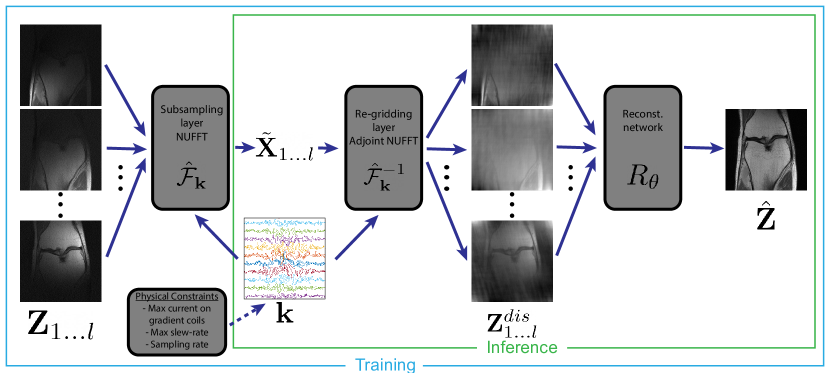
Figure 1: PILOT pipeline. Fully sampled multicoil images are inputs to the sub-sampling layer (NU-FFT) which samples the $k$-space along a trajectory $\mathbf{k}$. The measurements at the selected discrete set of frequencies are then passed to the regridding layer which performs a non-uniform Fast Fourier transform producing a space-domain image on a Cartesian grid. This image is then sent to the inverse model implemented as a reconstruction network (parameterized by $\bm{\mathrm{\theta}}$). Physical constraints on the trajectory $\bm{\mathrm{k}}$ are enforced at training.

It is convenient to view our approach as a single neural network combining the forward (acquisition) and the inverse (reconstruction) models (see Fig. 1 for a schematic depiction). The inputs to the model are the complex multi-channel fully sampled images, denoted as $\bm{\mathrm{Z}}$ with $l$ channels. The input is faced by a sub-sampling layer modeling the data acquisition along a $k$-space trajectory, a regridding layer producing an image on a Cartesian grid in the space domain, and an end-task model operating in the space domain and producing a reconstructed image (reconstruction task) or a segmentation mask (segmentation task).

In what follows, we detail each of the three ingredients of the PILOT pipeline. It should be mentioned that all of its components are differentiable with respect to the trajectory coordinates, denoted as $\bm{\mathrm{k}}$, in order to allow training the latter with respect to the performance of the end-task of interest.

2.1 Sub-sampling layer

The goal of the sub-sampling layer, denoted as $\hat{\mathcal{F}}_{\bm{\mathrm{k}}}$, is to create the set of measurements to be acquired by each one of the MRI scanner channels along a given trajectory in $k$-space. The trajectory is parametrized as a matrix $\bm{\mathrm{k}}$ of size $N_{\textrm{shots}}\times m$, where $N_{\textrm{shots}}$ is the number of RF excitations and $m$ is the number of sampling points in each excitation. The measurements themselves form a complex matrix of the same size emulated by means of non-uniform FFT (NU-FFT) (Dutt and Rokhlin, 1993) $\tilde{\bm{\mathrm{x}}}_{i}=\hat{\mathcal{F}}_{\bm{\mathrm{k}}}(\bm{\mathrm{Z}}_{i})$ on the full sampled complex images $\bm{\mathrm{Z}}_{i}\in\mathbb{C}^{n\times n}$ for each one of the $l$ channels ($1\leq i\leq l$). In the single-shot scenario, we refer to the ratio $n^{2}/m$ as the decimation rate (DR).

2.2 Regridding layer

For transforming non-Cartesian sampled MRI $k$-space measurements to the image domain we chose to use the adjoint non-uniform FFT (Dutt and Rokhlin, 1993), henceforth denoted as $\hat{\mathcal{F}}^{*}_{\bm{\mathrm{k}}}$. The non-uniform Fourier transform first performs regridding (resampling and interpolation) of the irregularly sampled points onto a regular grid followed by standard FFT. The result is a (distorted) MR image, $\bm{\mathrm{Z}}_{i}^{\textrm{dis}}=\hat{\mathcal{F}}^{*}_{\bm{\mathrm{k}}}(\tilde{\bm{\mathrm{x}}}_{i})$ for $1\leq i\leq l$.

Both the sub-sampling and the regridding layer contain an interpolation step. While it is true that the sampling operation is not differentiable (as it involves rounding non-integer values), meaningful gradients propagate through the bilinear interpolation module (a weighted average operation). For further details we refer the reader to Appendix A.

2.3 Task model

The goal of the task model is to extract the representation of the input images $\bm{\mathrm{Z}}_{1...l}^{\textrm{dis}}$ that will contribute the most to the performance of the end-task such as reconstruction or segmentation. At training, the task-specific performance is quantified by a loss function, which is described in Section 2.5. The model is henceforth denoted as $\hat{\bm{\mathrm{Z}}}=R_{\bm{\mathrm{\theta}}}(\bm{\mathrm{Z}}_{1...l}^{\textrm{dis}})$, with $\bm{\mathrm{\theta}}$ representing its learnable parameters. The input to the network is the distorted MR images, $\bm{\mathrm{Z}}_{1...l}^{\textrm{dis}}$, while the output varies according to the specific task. For example, in reconstruction, the output is an MR image (typically, on the same grid as the input), while in segmentation it is a mask representing the segments of the observed anatomy.

In the present work, to implement the task models we used a root-sum-of-squares layer (Larsson et al., 2003) followed by a multi-resolution encoder-decoder network with symmetric skip connections, also known as the U-Net architecture (Ronneberger et al., 2015). U-Net has been widely-used in medical imaging tasks in general as well as in MRI reconstruction (Zbontar et al., 2018) and segmentation (Isensee et al., 2017) in particular. It is important to emphasize that the principal focus of this work is not on the task model in se, since the proposed algorithm can be used with any differentiable model to improve the end task performance.

2.4 Physical constraints

A feasible sampling trajectory must follow the physical hardware constraint of the MRI machine, specifically the peak-current (translated into the maximum value of imaging gradients $G_{\mathrm{max}}$), along with the maximum slew-rate $S_{max}$ produced by the gradient coils. These requirements can be translated into geometric constraints on the first- and second-order derivatives of each of the spatial coordinates of the trajectory, $|\dot{k}|\approx\frac{|k_{i+1}-k_{i}|}{dt}\leq v_{\mathrm{max}}=\gamma\,G_{\mathrm{max}},$ and $|\ddot{k}|\approx\frac{|k_{i+1}-2k_{i}+k_{i-1}|}{dt^{2}}\leq a_{\mathrm{max}}=\gamma\,S_{\mathrm{max}},$ where $\gamma$ is the appropriate gyromagnetic ratio.

2.5 Loss function and training

The training of the proposed pipeline is performed by simultaneously learning the trajectory $\bm{\mathrm{k}}$ and the parameters of the task model $\bm{\mathrm{\theta}}$. A loss function is used to quantify how well a certain choice of the latter parameters performs, and is composed of two terms: a task fitting term and a constraints fitting term, $L=L_{\text{task}}+L_{\text{const}}.$

The aim of the first term is to measure how well the specific end task is performed. In the supervised training scenario, this term penalizes the discrepancy between the task-depended output of the model, $\hat{\bm{\mathrm{Z}}}$, and the desired ground truth outcome $\bm{\mathrm{Z}}$. For the reconstruction task, we chose the $L_{1}$ norm to measure the discrepancy between model output image $\hat{\bm{\mathrm{Z}}}$ and the ground-truth image $\bm{\mathrm{Z}}$, derived using the Root-Sum-of-Squares reconstruction (Larsson et al., 2003) of the fully sampled multi-channel images, $L_{\text{task}}=\|\hat{\bm{\mathrm{Z}}}-\bm{\mathrm{Z}}\|_{1}$. Similarly, for the segmentation task, we chose to use the cross-entropy operator to measure the discrepancy between the model output and the ground truth. This time, the model output $\hat{\bm{\mathrm{Z}}}$ was the estimated segmentation map while $\bm{\mathrm{Z}}$ is the ground truth segmentation map, The task loss is defined to be $L_{\text{task}}=H(\hat{\bm{\mathrm{Z}}},\bm{\mathrm{Z}})$, where $H$ is the cross-entropy loss. As was the case for the task model, our goal was not to find an optimal loss function for the task-fitting term, having in mind that the proposed algorithm can be used with more complicated loss function such as SSIM loss (Zhao et al., 2016) or a discriminator loss (Quan et al., 2018), as long as the latter is differentiable. The second term $L_{\text{const}}$ in the loss function applies to the trajectory $\bm{\mathrm{k}}$ only and penalizes for the violation of the physical constraints. We chose the hinge functions of the form $\mathrm{max}(0,|\dot{k}|-v_{\mathrm{max}})$ and $\mathrm{max}(0,|\ddot{k}|-a_{\mathrm{max}})$ summed over the trajectory spatial coordinates and over all sample points. These penalties remain zero as long as the solution is feasible and grow linearly with the violation of each of the constraints. The relative importance of the velocity (peak current) and acceleration (slew rate) penalties is governed by the parameters $\lambda_{v}$ and $\lambda_{a}$, respectively.

The training is performed by solving the optimization problem

$$\min_{\bm{\mathrm{k}},\bm{\mathrm{\theta}}}\,\sum_{(\bm{\mathrm{Z_{1...l}}},\bm{\mathrm{Z}})}L_{\text{task}}(R_{\bm{\mathrm{\theta}}}(\hat{\mathcal{F}}^{*}_{\bm{\mathrm{k}}}(\hat{\mathcal{F}}_{\bm{\mathrm{k}}}(\bm{\mathrm{Z_{1...l}}}))),\bm{\mathrm{Z}})+L_{\text{const}}(\bm{\mathrm{k}}),$$ (1)

where the loss is summed over a training set comprising the pairs of fully sampled data $\bm{\mathrm{Z_{1...l}}}$ and the corresponding groundtruth output $\bm{\mathrm{Z}}$.

2.6 Extensions

Since optimization problem (1) is highly non-convex, iterative solvers are guaranteed to converge only locally. Indeed, we noticed that the learned trajectory $\bm{\mathrm{k}}$ significantly depends on the initialization. To overcome this difficulty we propose the following two methods to improve the algorithm exploration and finding solutions closer to the global minimum of Eq. 1.

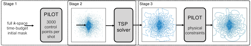
Figure 2: PILOT-TSP training pipeline. At the first stage, an unordered set of $k$-space points is learned without enforcing any hardware constraints. At the second stage, a greedy solver to the traveling salesman problem is employed to construct a trajectory passing through the sampled points. At the final stage, the obtained trajectory is used as the initialization the PILOT training pipeline with physical constraints enforced during training.

2.6.1 PILOT-TSP

A naive way to mitigate the effect of such local convergence is to randomly initialize the trajectory coordinates. However, our experiments show that random initialization invariably result in sequences of points that are far from each other and, thus, induce huge velocities and accelerations violating the constraints by a large margin. The minimization of the previously described loss function with such an initialization appears to be unstable and does not produce useful solutions.

To overcome this difficulty, we introduce PILOT-TSP, an extension of PILOT for optimizing single-shot trajectories from random initialization. TSP stands for the Traveling Salesmen Problem, in our terminology, TSP aims at finding an ordering of $m$ given $k$-space coordinates such that the path connecting them has minimal length. Since TSP is NP-hard, we used a greedy approximation algorithm (Grefenstette et al., 1985) for solving it, as implemented in TSP-Solver. Using this approach, we first optimize for the best unconstrained solution (i.e., the weights of the $L_{\mathrm{const}}$ term in the loss are set to zero), and then find the closest solution satisfying the constraints.

The flow of PILOT-TSP, described schematically in Fig. 2, proceeds in four consecutive stages, as follows:

1. Trajectory coordinates $\bm{\mathrm{k}}$ are initialized by sampling $m$ i.i.d. vectors from a normal distribution with zero mean and standard deviation of $\sigma=\frac{n}{6}$;

2. The parameters $\bm{\mathrm{k}}$ of the trajectory and $\bm{\mathrm{\theta}}$ of the task model are optimized by solving (1) with the second loss term set to zero. Note that this makes the solution independent of the ordering of $\bm{\mathrm{k}}$.

3. Run the TSP approximate solver to order the elements of the vector $\bm{\mathrm{k}}$ and form the trajectory. This significantly reduces albeit still does not completely eliminate constraint violation, as can be seen in the input to stage 3 in Fig. 2.

4. The trajectory is fine-tuned to obey the constraints by further performing iteration on the loss in (1) this time with the constraints term.

It is important to note that unlike previous works using TSP for trajectory optimization, that modify the target sampling density (Wang et al., 2012; Chauffert et al., 2014), in our work it is used only for the purpose of reordering the existing sampling points without any resampling along the trajectory (stage 3 above), therefore the sampling density remains unchanged after TSP.

2.6.2 Multi-scale PILOT

Experimentally, we observed that enforcing all the points as free optimization variables do not cause “global” changes in the trajectory shape. One technique that proved effective to overcome this limitation is to learn only a subset of points that we refer to as control points, with the rest of the trajectory interpolated using a differentiable cubic spline. This method showed more “global” changes but less “randomly” spread points as proven to improve performance (Lustig et al., 2007). To compromise between the “global” and the “local” effects, we adopted a multi-scale optimization approach. In this approach, we start from optimizing over a small set of control points per shot, and gradually increase their amount as the training progresses until all the trajectory points are optimized (e.g. starting from 60 points per shot with 3000 points and double their amount every 5 epochs). It is important to note that we enforce the feasibility constraints on the trajectory after the spline interpolation in order to keep the trajectory feasible during all the optimization steps.

3 Experiments and Discussion

3.1 Datasets

We used two datasets in the preparation of this article: the NYU fastMRI initiative database (Zbontar et al., 2018), and the medical segmentation decathlon (Simpson et al., 2019). The fastMRI dataset contains raw knee MRI volumes with 2D spatial dimensions of $320\times 320$. The fastMRI dataset consists of data obtained from multiple machines through two pulse sequences: proton-density and proton-density fat suppression. We included only the proton-density volumes in our dataset. Since our work focuses on designing $k$-space trajectories and the provided test set in fastMRI is already sub-sampled, we split the training set into two sets: one containing $484$ volumes ($17000$ slices) for training and validation (80/20 split), and $100$ volumes ($3500$ slices) for testing. Furthermore, the fastMRI dataset is acquired from multiple 3T scanners (Siemens Magnetom Skyra, Prisma, and Biograph mMR) as well as 1.5T machines (Siemens Magnetom Aera). All data were acquired through the fully-sampled Cartesian trajectories using the 2D TSE protocol.

For the segmentation task, we used data obtained from the medical image segmentation decathlon challenge (Simpson et al., 2019). Within the decathlon challenge, we used the brain tumors dataset that contained $750$ 4D volumes (of $k$-space size $256\times 256$) of multi-modal (FLAIR, T1w, T1gd & T2w) brain MRI scans from patients diagnosed with either glioblastoma or lower-grade glioma. Gold standard annotations for all tumor regions in all scans were approved by expert board-certified neuroradiologists as detailed in Simpson et al. (2019). Within this dataset, we used only the T2-weighted images. Since the goal of our experiment is to design trajectories that are optimal for segmenting tumors, we only considered images containing tumors, and used only the training set for all the experiments since they are the only ones that contain ground-truth segmentations. These data were split into two sets: one containing $400$ volumes ($26000$ slices) for training and validation, and the other one containing $84$ volumes ($5300$ slices) for testing. We emphasize that, due to the unavailability of the segmentation dataset that consists of true $k$-space data, for this experiment, we use the simulated $k$-space data obtained from the images. We believe that although the data are simulated, they can still be used in a proof-of-concept experiment.

Table 1: Comparison of fixed and learned trajectories in the single-shot setting for image reconstruction. Presented are the PSNR and SSIM metrics of the fixed and learned trajectories for different decimation rates (DR). Reported baselines: fixed spiral trajectory (Spiral-Fixed), PILOT initialized with spiral (Spiral-PILOT), and the PILOT-TSP algorithm (PILOT-TSP).

DR	Trajectory	Spiral-Fixed	Spiral-PILOT	PILOT-TSP
10	PSNR	28.16$\pm$1.43	31.87$\pm$1.47	32.07$\pm$1.43
	SSIM	0.734$\pm$0.041	0.814$\pm$0.035	0.824$\pm$0.032
20	PSNR	24.08$\pm$1.50	29.64$\pm$1.44	30.25$\pm$1.48
	SSIM	0.591$\pm$0.052	0.761$\pm$0.039	0.776$\pm$0.040
80	PSNR	21.05$\pm$1.61	24.31$\pm$1.49	26.37$\pm$1.50
	SSIM	0.478$\pm$0.049	0.598$\pm$0.048	0.657$\pm$0.048

3.2 Training settings

We trained both the sub-sampling layer and the task model network with the Adam (Kingma and Ba, 2014) solver. The learning rate was set to $0.001$ for the task model, while the sub-sampling layer was trained with learning rates varying between $0.001$ to $0.1$ in different experiments. The parameters $\lambda_{v}$ and $\lambda_{a}$ were set to $0.1$. We implemented the differentiable NUFFT and adjoint-NUFFT layers using pytorch’s autograd tools (Paszke et al., 2019), by adapting the code available in the sigpy package. In both these layers, we use the Kaiser-Bessel kernel with oversampling factor set to 1.25, and interpolation kernel width (in terms of oversampled grid) set to 4.

3.3 Physical constraints

The following physical constraints were used in all our experiments: $G_{\mathrm{max}}=$ 40mT/m for the peak gradient, $S_{\mathrm{max}}=$ 200T/m/s for the maximum slew-rate, and $dt=10\mu$sec for the sampling time.

3.4 Image reconstruction

In order to quantitatively evaluate our method, we use the peak signal-to-noise ratio (PSNR) and the structural-similarity measures (SSIM) (Zhou Wang et al., 2004), portraying both the pixel-to-pixel and perceptual similarity. In all our experiments, we compare our algorithms to the baseline of training only the reconstruction model for measurements obtained with fixed handcrafted trajectories, henceforth referred to as “fixed trajectory”.

3.4.1 Single-shot trajectories

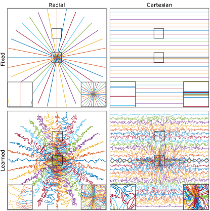
Figure 3: Multi-shot PILOT trajectories. Comparison of fixed (top) and learned (bottom) $k$-space trajectories for the radial (left) and Cartesian (right) initialization with $N_{\textrm{shots}}=16,32$ respectively. The learned trajectories obey the following constraints: maximum gradient $G_{\text{max}}=40\,\text{mT/m}$, maximum slew-rate $S_{\text{max}}=200\,\text{T/m/s}$ and sampling interval $dt=10\,\mu s$.

For the single-shot setting, we used the spiral trajectory (Block and Frahm, 2005; Meyer et al., 1992) both as the baseline and the initialization to our model. We also used random initialization with PILOT-TSP, as described in Section 2.6.1, initialized with . In order to initialize feasible spirals that obey the hardware constraints, we used the variable-density spiral design toolbox available in , which produces spirals covering the $k$-space with the length of $m$ samples. Table 1 presents quantitative results comparing fixed spiral initialization to PILOT. The results demonstrate that PILOT outperforms the fixed trajectory across all decimation rates. As mentioned in Section 2.1, the decimation rate (DR) is calculated as the ratio between the total grid size of the $k$-space ($n^{2}$) divided by the number of points sampled in the shot ($m$), i.e., $\textrm{DR}=n^{2}/m$. The observed improvement is in the range of $3.26-5.56$ dB PSNR and $0.080-0.170$ SSIM points.

Table 1 also summarizes the quantitative results of PILOT-TSP. We observe that PILOT-TSP provides improvements in the range of $0.2-2.06$dB PSNR and $0.010-0.059$ SSIM points when compared to the learned trajectory with the spiral initialization and a total of $3.91-6.17$dB PSNR and $0.090-0.185$ SSIM points overall improvement over fixed trajectories. Examples of PILOT-TSP trajectories can be seen in Figs 7 and 6.

3.4.2 Multi-shot trajectories

	PSNR	SSIM
Fixed	29.09$\pm$1.43	0.741$\pm$0.040
PILOT (without multi-scale)	31.93$\pm$1.52	0.818$\pm$0.036
PILOT (with multi-scale)	33.71$\pm$1.58	0.863$\pm$0.032

Table 2: Multi-scale PILOT. Comparison of PILOT with and without multi-scale optimization for the radial initialization with $N_{\textrm{shots}}=16$.

In the multi-shot scenario, we used Cartesian, radial (Lauterbur, 1973) and spiral (Meyer et al., 1992) trajectories both as the baseline and as the initialization for PILOT. We denote the number of shots as $N_{\textrm{shots}}$, each containing $3000$ samples corresponding to the readout time of $30ms$. As mentioned in Section 2.6.2 we observed that using PILOT with multi-scale optimization lead to better performance. Therefore, in this work all multi-shot experiments use multi-scale optimization. Table 2 shows a comparison between PILOT with and without multi-scale optimization. Table 3 presents the quantitative results comparing fixed trajectories to PILOT with the same initialization. The results demonstrate that in the multi-shot setting, as well, PILOT outperforms the fixed trajectory. In Fig. 3 in the Cartesian setting, we can notice how the learned trajectory has much better coverage of the $k$-space which in turn led to huge improvement is in the range of $6.14-6.99$ dB PSNR and $0.161-0.172$ SSIM points. In the radial case, PILOT observes an improvement in the range of $3.31-4.99$ dB PSNR and $0.086-0.138$ SSIM points, and for spiral we see improvement in the range of $1.66-3.16$ dB PSNR and $0.029-0.084$ SSIM points.

More interestingly, for spiral initialization PILOT applied to the fewer shots setups ($4$ and $8$) surpasses the performance of the fixed trajectory setups with a higher number of shots ($8$ and $16$). For Cartesian and radial initializations, PILOT with as little as $8$ shots surpasses the $32$ fixed trajectory. This indicates that by using PILOT one can achieve about two to four times shorter acquisition without compromising the image quality (without taking into account additional acceleration potential due to the reconstruction network).

An example of fixed and learned trajectories is presented in Figure 3. Gradient and slew rate of one of the learned trajectories can be seen in Fig. 4. Fig. 5 shows a visual comparison of the distorted and reconstructed images using fixed and learned trajectories, it is interesting to observe the improvement in the distorted images which depend only on the trajectories.
The learned trajectories enjoy two main advantages over the traditional (”handcrafted”) trajectories:

1. The sampling points ”adapt” (in a data-driven manner) to the sampling density of the specific organ, task, and task model (e.g. reconstruction method for reconstruction).

2. The sampling points ”jitter” around the trajectory in order to get better k-space coverage in multiple directions. This result resembles CAIPIRINHA-like zig-zag sampling that is traditionally handcrafted for parallel MR imaging (Breuer et al., 2005).

Table 3: Comparison of fixed and learned trajectories in the multi-shot setting for image reconstruction. Presented are the PSNR and SSIM metrics of fixed and learned trajectories for different number of shots ($N_{\textrm{shots}}=4,8,16,32$). Reported baselines: fixed spiral, radial, Cartesian trajectories (denoted by Spiral-Fixed, Radial-Fixed and Cartesian-Fixed, respectively); PILOT initialized with spiral, radial and Cartesian trajectories (denoted by Spiral-PILOT, Radial-PILOT and Cartesian-PILOT, respectively).

$N_{\textrm{shots}}$	4		8
Trajectory	PSNR	SSIM	PSNR	SSIM
Cartesian-Fixed1	-	-	24.45$\pm$1.44	0.622$\pm$0.044
Cartesian-PILOT1	-	-	31.13$\pm$1.44	0.785$\pm$0.035
Radial-Fixed1	-	-	27.24$\pm$1.41	0.686$\pm$0.044
Radial-PILOT1	-	-	32.41$\pm$1.48	0.824$\pm$0.035
Spiral-Fixed	29.05$\pm$1.59	0.747$\pm$0.046	31.88$\pm$1.54	0.831$\pm$0.031
Spiral-PILOT	32.21$\pm$ 1.50	0.831$\pm$0.036	34.54$\pm$1.46	0.876$\pm$0.033
$N_{\textrm{shots}}$	16		32
Trajectory	PSNR	SSIM	PSNR	SSIM
Cartesian-Fixed	24.93$\pm$1.48	0.639$\pm$0.043	27.78$\pm$1.44	0.711$\pm$0.042
Cartesian-PILOT	31.92$\pm$1.44	0.811$\pm$0.035	33.92$\pm$1.62	0.872$\pm$0.031
Radial-Fixed	29.09$\pm$1.43	0.741$\pm$0.040	31.09$\pm$1.48	0.798$\pm$0.037
Radial-PILOT	33.71$\pm$1.58	0.863$\pm$0.032	34.40$\pm$1.58	0.884$\pm$0.029
Spiral-Fixed2	33.89$\pm$1.56	0.874$\pm$0.030	-	-
Spiral-PILOT2	35.55$\pm$1.59	0.903$\pm$0.026	-	-

• ¹For $N_{\textrm{shots}}=4$, fixed Cartesian trajectories and fixed radial trajectories result in a very poor performance probably because of their poor coverage in the $k$-space, therefore we omit the results for these baselines for both fixed and learned trajectory baselines.

• ²Spiral trajectory with $N_{\textrm{shots}}=32$ resulted in less than 3000 sampling points per shot and was therefore omitted for a consistent comparison.

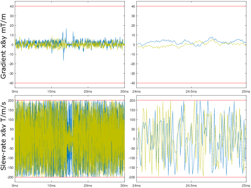
Figure 4: Gradient (top) and slew-rate (bottom) plots of the learned $k$-space trajectory with radial initialization for $N_{\textrm{shots}}=16$. The right column depicts a zoom-in portion. The red lines are the constraints used in the optimization: maximum gradient $G_{\text{max}}=40\,\text{mT/m}$, maximum slew-rate $S_{\text{max}}=200\,\text{T/m/s}$.

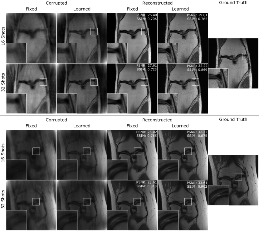
Figure 5: Image reconstruction with PILOT. Compared are the fixed and learned trajectories for radial initialization with 16 (top row) and 32 shots (bottom row). Columns 1 & 2 depict the images after resampling (root-sum-of-squares) and depicted in columns 3 & 4 are the reconstructed images. The groundtruth image obtained from the fully sampled $k$-space is depicted in the rightmost column. PSNR and SSIM scores for the reconstructed images are reported alongside with zoom-in region displaying important anatomical details.

3.5 Optimal trajectory design for segmentation

We demonstrate the ability of the proposed methods to learn a trajectory optimized for a specific end-task on the tumor segmentation task. The details of the dataset used are described in Section 3.1. We use the standard Dice similarity coefficient (DICE) and the intersection-over-union (IOU) metrics to quantify segmentation accuracy.

The results for segmentation are reported in Table 4. We observe that the learned trajectories achieve an improvement of $0.015-0.044$ DICE points and $0.018-0.056$ IOU points when compared to the fixed trajectories they were initialized with. Visual comparison of the described results is available in Fig.6. We emphasize that since the dataset for the segmentation task was likely post-processed and therefore the retrospective data acquisition simulation is not as accurate as in the case of reconstruction task where the raw multi-channel $k$-space data was available. Nevertheless, the margins achieved in reconstruction experiments encourage us to believe that similar margins would be obtained on the segmentation task as well when trained with raw $k$-space data as the input.

Table 4: Comparison of fixed and learned trajectories in the single-shot setting for the tumor segmentation task. Presented are the DICE and IOU metrics of the fixed and learned trajectories for different decimation rates (DR). Reported baselines: fixed spiral trajectory (Spiral-Fixed), PILOT initialized with spiral (Spiral-PILOT), and the PILOT-TSP algorithm (PILOT-TSP). Three different decimation rates are reported.

DR	Trajectory	Spiral-Fixed	Spiral-PILOT	PILOT-TSP
10	DICE	0.810$\pm$0.012	0.825$\pm$0.011	0.816$\pm$0.009
	IOU	0.719$\pm$0.015	0.737$\pm$0.014	0.726$\pm$0.012
20	DICE	0.774$\pm$0.016	0.811$\pm$0.016	0.818$\pm$0.017
	IOU	0.669$\pm$0.017	0.716$\pm$0.016	0.725$\pm$0.016
80	DICE	0.720$\pm$0.022	0.735$\pm$0.019	0.754$\pm$0.018
	IOU	0.611$\pm$0.019	0.626$\pm$0.016	0.639$\pm$0.017

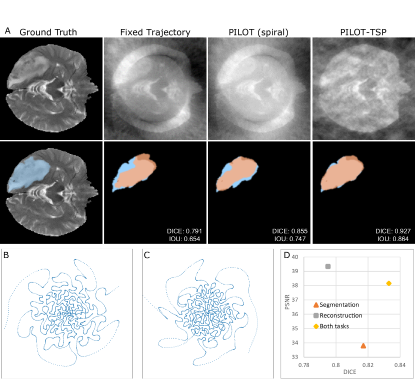
Figure 6: Tumor segmentation. (A) Compared are the fixed spiral trajectory (second column), PILOT with spiral initialization (third column), and PILOT-TSP (rightmost column). The first row depicts the MR images as obtained after the inverse Fourier transform with no further processing. The groundtruth image obtained from the fully sampled $k$-space is depicted in the leftmost column. The second row depicts the predicted segmentation map (red) and the groundtruth map (blue) with the corresponding DICE and IOU scores. (B, C) shows comparison of the learned trajectories optimized for different tasks: segmentation (B) and reconstruction (C). (D) Quantitative performance of trajectories optimized with different end-task (reconstruction, segmentation and both together) on both tasks - reconstruction (PSNR) and segmentation (DICE)

3.6 Cross-task and multi-task learning

In order to verify end-task optimality of the found solution, we evaluated the learned models on tasks they were not learned on. Specifically, we trained PILOT-TSP with the same dataset once on the segmentation task and another time on the reconstruction task. We then swapped the obtained trajectories between the tasks, fixed them, and re-trained only the task model (U-Net) for each task (while keeping the trajectory as it was learned for the other task). The results for this experiment are reported in Fig. 6. We observe that the trajectories obtained from segmentation are optimal for that task alone and perform worse on reconstruction, and vice-versa. From the output trajectories learned for segmentation and reconstruction, visualized in Fig 6, we can see that the reconstruction trajectory is more centered around the DC frequency, whereas the segmentation trajectory tries to cover higher frequencies. This could be explained by the fact that most of the image information is contained within the lower frequencies in the $k$-space, therefore covering them, contributes more to the pixel-wise similarity measure of the reconstruction task. For the segmentation task, contrarily, the edges and the structural information present in the higher frequencies, is more critical for the success of the task. This is an interesting observation because it paves the way to design certain accelerated MRI protocols that are optimal for a given end-task that is not necessarily image reconstruction.

Another important use can be to jointly learn several tasks such as segmentation and reconstruction in order to find the best segmentation while preserving the ability to reconstruct a meaningful human-intelligible image. For this purpose, we build a model with one encoder and two separate decoders (separated at the bottleneck layer of the U-Net), each for a different task. The loss function is defined to be the sum of both the reconstruction loss (from the first decoder) and the segmentation loss (pixel-wise cross-entropy, from the second decoder). The results for this experiment are reported in Fig. 6. Interestingly, we can observe that the presence of the reconstruction tasks aids segmentation as well. This is also consistent with the results observed in Sun et al. (2018).

3.7 Comparison with prior art

SPARKLING (Lazarus et al., 2019a) is the state-of-the-art method for single-shot 2D k-space optimization under gradient amplitude and slew constraints, we use it for comparative evaluation of PILOT. A single-shot trajectory corresponding to decimation rate $20$ was generated using the variable density sampling density suggested in the paper, using the implementation provided in Lebrat et al. (2019), an extension of SPARKLING. We tested the performance of both trajectories with U-Net as the reconstruction methods, trained for each trajectory. Figure 7 displays SPARKLING and PILOT-TSP generated trajectories and the quantitative results. As can be inferred from the results, PILOT outperforms SPARKLING with $1.15$ dB PSNR and $0.030$ SSIM points. We assume the reason for the superior performance of PILOT when compared to SPARKLING is mainly due to PILOT’s data-driven approach for selecting the sampling points. SPARKLING tries to fit the trajectory to a “handcrafted” pre-determined sampling density, where as in PILOT the sampling density is implicitly optimized together with the trajectory to maximize the performance of the end task.

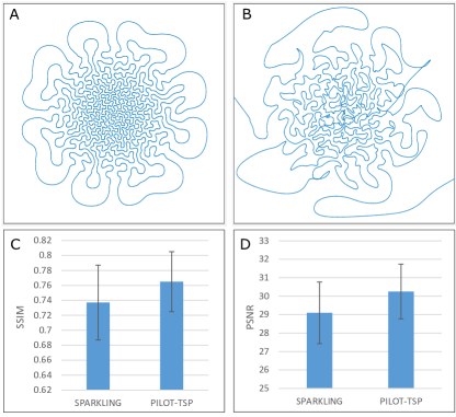
Figure 7: Comparison of SPARKLING (A) and PILOT-TSP (B) trajectories for decimation rate of 20 with evaluation of the reconstruction using U-Net (C, D).

3.8 Resilience to noise

In order to test the effect of measurement noise on the performance of PILOT trajectories, we designed the following twofold experiment: (1) emulated the lower SNR only in the test samples using trajectories trained without the noise (w/o retraining); and (2) emulating the lower SNR both in train and test samples (with retraining).
SNR emulation. In order to emulate measurement noise we added white Gaussian noise to the real and imaginary parts of each of the input channels. We used noise with higher variance to emulate lower SNR. The results are summarized in Fig. 8. We observe the relative advantage of PILOT in both scenarios, with and without training over low SNR samples, while for the latter the learned trajectory and model are more resilient in the presence of noise. We assume that this improvement is both due to the adaptation of the reconstruction network and due to trajectory adaptation to the lower SNR. Learned trajectories in the presence of different SNR values can be seen in Fig. 8, we can see that in the higher SNR case the sampling points are more dispersed over the $k$-space than in the lower SNR case. This is probably due to the need to average many close sampling points in order to counter the noise.

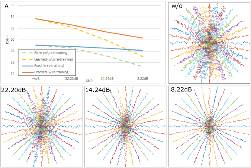
Figure 8: Comparison of PILOT with radial initialization with and without accounting for lower SNR. The dashed lines (yellow and green) in sub-figure A correspond to the performance when the SNR decay was emulated only during inference, i.e., the models were trained without accounting for the lower SNR. The continuous lines (orange and blue) in sub-figure A presents the performance of the models when trained with lower SNR. The effect of the SNR on the learned trajectories can be seen in the trajectories plots, the upper-right trajectory trained without noise and the bottom trajectories were trained with different levels of SNR.

4 Conclusion and future directions

We have demonstrated, as a proof-of-concept, that learning the $k$-space sampling trajectory simultaneously with an image reconstruction neural model improves the end image quality of an MR imaging system. To the best of our knowledge, the proposed PILOT algorithm is the first to do end-to-end learning over the space of all physically feasible MRI 2D $k$-space trajectories. We also showed that end-to-end learning is possible with other tasks such as segmentation. On both tasks and across decimation rates and initializations PILOT manages to learn physically feasible trajectories which demonstrates significant improvement over the fixed counterparts. We proposed two extensions to the PILOT framework, namely, multi-scale PILOT and PILOT-TSP in order to partially alleviate the local minima that are prevalent in trajectory optimization. We further studied the robustness of our learned trajectories and reconstruction model in the presence of SNR decay.
Below we list some limitations of the current work and some future directions:

• In this paper, we only validated our method through retrospective acquisitions, we hope to validate it prospectively by deploying the learned trajectories on a real MRI machine.

• We were unable to obtain a segmentation dataset containing the raw $k$-space data, we plan to obtain such datasets and evaluate the performance of our methods on them.

• Adding echo time (TE) constraints in order to control the received contrast.

• Considering a more accurate physical model accounting for eddy current effects (e.g. gradient impulse response function (GIRF) model (Vannesjo et al., 2013)).

• We did not evaluate the robustness of our trajectories to off-resonance effects. Preliminary simulation results in Lazarus et al. (2019a) suggested that similarly optimized trajectories are more robust to off-resonance effects when compared to spiral. In future work, we will evaluate the robustness of PILOT by performing similar simulations.

• Extending PILOT-TSP to multi-shot trajectories.

Acknowledgments

This work was supported by the ERC CoG EARS.

Ethical Standards

The work follows appropriate ethical standards in conducting research and writing the manuscript, following all applicable laws and regulations regarding treatment of animals or human subjects.

Conflicts of Interest

We declare we don’t have conflicts of interest.

Appendix A.

In what follows we describe the implementation of the differentiable interpolation step used in the sub-sampling and regridding layers. Let us assume we know the value of a function $f$ on a discrete grid, $X=\{i\in 1...n\},f(i)=y_{i}$ and we would like to evaluate the value of $f$ at a point $z$ that does not lie on the grid. We perform this operation in two steps:

1. Find the points in $X$ that satisfy $\{j,j+1\in X\,|\,j=\text{floor}(z)\}$. This step is indeed piecewise differentiable with respect to $z$: the gradient is defined and equals zero outside the set $X$ and is not defined otherwise. Therefore the gradient is zero almost everywhere.

2. Now we define a function $f_{cont}$, an interpolation function, to estimate the value of the function $f$ at $z$, $f_{cont}(z)=(z-j)f(j)+(j+1-z)f(j+1)$. This step is differentiable with respect to z.

The function $f_{cont}$ is the function defined on the real domain and it is equal to the discrete function $f$ when the input is an integer. Let us now evaluate the derivative of $f_{cont}$ w.r.to $z$

$$\frac{\partial f_{cont}}{\partial z}=f(j)-f(j+1)+(z-j)f^{\prime}(j)\frac{\partial j}{\partial z}+(j+1-z)f^{\prime}(j+1)\frac{\partial j}{\partial z}$$

and since, $j=\text{floor}(z)$ has $\frac{\partial j}{\partial z}=0,\forall z\notin X$ and undefined elsewhere we assume $\frac{\partial j}{\partial z}=0$. This yields $\frac{\partial f_{cont}}{\partial z}=f(j)-f(j+1)$. While in this example we considered the simple case of linear interpolation, the general logic applies for higher-order or kernel-based interpolation techniques as well. In our implementation, however, we did not use this kind of direct approach for the calculation of the gradient, instead we used the autograd engine available in pytorch (Paszke et al., 2019) for this purpose.

References

- Adcock et al. (2017) Ben Adcock, Anders C Hansen, Clarice Poon, and Bogdan Roman. Breaking the coherence barrier: A new theory for compressed sensing. In Forum of Mathematics, Sigma, volume 5. Cambridge University Press, 2017.
- Aggarwal and Jacob (2020) Hemant K Aggarwal and Mathews Jacob. Joint optimization of sampling pattern and priors in model based deep learning. In 2020 IEEE 17th International Symposium on Biomedical Imaging (ISBI), pages 926–929. IEEE, 2020.
- Alush-Aben et al. (2020) Jonathan Alush-Aben, Linor Ackerman, Tomer Weiss, Sanketh Vedula, Ortal Senouf, and Alex Bronstein. 3d flat-feasible learned acquisition trajectories for accelerated mri. 2020.
- Bahadir et al. (2019) Cagla D. Bahadir, Adrian V. Dalca, and Mert R. Sabuncu. Adaptive compressed sensing MRI with unsupervised learning. arXiv e-prints, art. arXiv:1907.11374, Jul 2019.
- Bahadir et al. (2019) Cagla Deniz Bahadir, Adrian V Dalca, and Mert R Sabuncu. Learning-based optimization of the under-sampling pattern in mri. In International Conference on Information Processing in Medical Imaging, pages 780–792. Springer, 2019.
- Block and Frahm (2005) Kai Tobias Block and Jens Frahm. Spiral imaging: A critical appraisal. Journal of Magnetic Resonance Imaging, pages 657–668, 2005. doi: 10.1002/jmri.20320.
- Boyer et al. (2019) Claire Boyer, Jérémie Bigot, and Pierre Weiss. Compressed sensing with structured sparsity and structured acquisition. Applied and Computational Harmonic Analysis, 46(2):312–350, 2019.
- Breuer et al. (2005) Felix A Breuer, Martin Blaimer, Robin M Heidemann, Matthias F Mueller, Mark A Griswold, and Peter M Jakob. Controlled aliasing in parallel imaging results in higher acceleration (caipirinha) for multi-slice imaging. volume 53, pages 684–691. Wiley Online Library, 2005.
- Candes et al. (2006) Emmanuel J Candes, Justin K Romberg, and Terence Tao. Stable signal recovery from incomplete and inaccurate measurements. Communications on Pure and Applied Mathematics: A Journal Issued by the Courant Institute of Mathematical Sciences, 59(8):1207–1223, 2006.
- Chauffert et al. (2013) Nicolas Chauffert, Philippe Ciuciu, and Pierre Weiss. Variable density compressed sensing in mri. theoretical vs heuristic sampling strategies. In 2013 IEEE 10th International Symposium on Biomedical Imaging, pages 298–301. IEEE, 2013.
- Chauffert et al. (2014) Nicolas Chauffert, Philippe Ciuciu, Jonas Kahn, and Pierre Weiss. Variable density sampling with continuous trajectories. SIAM Journal on Imaging Sciences, pages 1962–1992, 2014.
- Dar et al. (2020) S. U. H. Dar, M. Yurt, M. Shahdloo, M. E. Ildız, B. Tınaz, and T. Çukur. Prior-guided image reconstruction for accelerated multi-contrast mri via generative adversarial networks. IEEE Journal of Selected Topics in Signal Processing, 14(6):1072–1087, 2020. doi: 10.1109/JSTSP.2020.3001737.
- Dar et al. (2020) Salman Ul Hassan Dar, Muzaffer Özbey, Ahmet Burak Çatlı, and Tolga Çukur. A transfer-learning approach for accelerated mri using deep neural networks. Magnetic Resonance in Medicine, 84(2):663–685, 2020.
- Dutt and Rokhlin (1993) A. Dutt and V. Rokhlin. Fast fourier transforms for nonequispaced data. SIAM J. Sci. Comput., pages 1368–1393, 1993.
- Ferguson (1964) James Ferguson. Multivariable curve interpolation. Journal of the ACM (JACM), pages 221–228, 1964.
- Gözcü et al. (2018) Baran Gözcü, Rabeeh Karimi Mahabadi, Yen-Huan Li, Efe Ilıcak, Tolga Çukur, Jonathan Scarlett, and Volkan Cevher. Learning-based compressive MRI. IEEE, Transactions on Medical Imaging, pages 1394–1406, 2018.
- Grefenstette et al. (1985) John J. Grefenstette, Rajeev Gopal, Brian J. Rosmaita, and Dirk Van Gucht. Genetic algorithms for the traveling salesman problem. In ICGA, pages 160–168, 1985.
- Hammernik et al. (2018) Kerstin Hammernik, Teresa Klatzer, and Erich et al. Kobler. Learning a variational network for reconstruction of accelerated MRI data. Magnetic Resonance in Medicine, pages 3055–3071, 2018.
- Isensee et al. (2017) Fabian Isensee, Paul F Jaeger, Peter M Full, Ivo Wolf, Sandy Engelhardt, and Klaus H Maier-Hein. Automatic cardiac disease assessment on cine-MRI via time-series segmentation and domain specific features. In International workshop on statistical atlases and computational models of the heart. Springer, 2017.
- Kingma and Ba (2014) Diederik P. Kingma and Jimmy Ba. ADAM: A Method for Stochastic Optimization. arXiv e-prints, art. arXiv:1412.6980, Dec 2014.
- Knoll et al. (2011) Florian Knoll, Christian Clason, Clemens Diwoky, and Rudolf Stollberger. Adapted random sampling patterns for accelerated mri. Magnetic resonance materials in physics, biology and medicine, 24(1):43–50, 2011.
- Krahmer and Ward (2013) Felix Krahmer and Rachel Ward. Stable and robust sampling strategies for compressive imaging. IEEE transactions on image processing, 23(2):612–622, 2013.
- Larsson et al. (2003) Erik G Larsson, Deniz Erdogmus, Rui Yan, Jose C Principe, and Jeffrey R Fitzsimmons. SNR-optimality of sum-of-squares reconstruction for phased-array magnetic resonance imaging. Journal of Magnetic Resonance, pages 121–123, 2003.
- Lauterbur (1973) P. C. Lauterbur. Image formation by induced local interactions: Examples employing nuclear magnetic resonance. Nature, pages 190–191, Mar 1973. doi: 10.1038/242190a0.
- Lazarus et al. (2019a) Carole Lazarus, Pierre Weiss, and Nicolas et al. Chauffert. SPARKLING: variable-density k-space filling curves for accelerated T2*-weighted MRI. Magnetic Resonance in Medicine, pages 3643–3661, 2019a. doi: 10.1002/mrm.27678.
- Lazarus et al. (2019b) Carole Lazarus, Pierre Weiss, Loubna Gueddari, Franck Mauconduit, Alexandre Vignaud, and Philippe Ciuciu. 3d sparkling trajectories for high-resolution t2*-weighted magnetic resonance imaging. 2019b.
- Lebrat et al. (2019) Léo Lebrat, Frédéric de Gournay, Jonas Kahn, and Pierre Weiss. Optimal transport approximation of 2-dimensional measures. SIAM Journal on Imaging Sciences, 12(2):762–787, 2019.
- Likes (1981) Richard S Likes. Moving gradient zeugmatography, December 22 1981. US Patent 4,307,343.
- Lustig and Pauly (2010) Michael Lustig and John M Pauly. Spirit: iterative self-consistent parallel imaging reconstruction from arbitrary k-space. Magnetic resonance in medicine, 64(2):457–471, 2010.
- Lustig et al. (2007) Michael Lustig, David Donoho, and John M Pauly. Sparse MRI: The application of compressed sensing for rapid MR imaging. Magnetic Resonance in Medicine, pages 1182–1195, 2007.
- Meyer et al. (1992) Craig H Meyer, Bob S Hu, Dwight G Nishimura, and Albert Macovski. Fast spiral coronary artery imaging. Magnetic resonance in medicine, pages 202–213, 1992.
- Paszke et al. (2019) Adam Paszke, Sam Gross, Francisco Massa, Adam Lerer, James Bradbury, Gregory Chanan, Trevor Killeen, Zeming Lin, Natalia Gimelshein, Luca Antiga, Alban Desmaison, Andreas Kopf, Edward Yang, Zachary DeVito, Martin Raison, Alykhan Tejani, Sasank Chilamkurthy, Benoit Steiner, Lu Fang, Junjie Bai, and Soumith Chintala. Pytorch: An imperative style, high-performance deep learning library. In H. Wallach, H. Larochelle, A. Beygelzimer, F. d'Alché-Buc, E. Fox, and R. Garnett, editors, Advances in Neural Information Processing Systems 32, pages 8024–8035. Curran Associates, Inc., 2019. URL http://papers.neurips.cc/paper/9015-pytorch-an-imperative-style-high-performance-deep-learning-library.pdf.
- Puy et al. (2011) Gilles Puy, Pierre Vandergheynst, and Yves Wiaux. On variable density compressive sampling. IEEE Signal Processing Letters, 18(10):595–598, 2011.
- Quan et al. (2018) T. M. Quan, T. Nguyen-Duc, and W. Jeong. Compressed sensing mri reconstruction using a generative adversarial network with a cyclic loss. IEEE Transactions on Medical Imaging, 2018.
- Ronneberger et al. (2015) Olaf Ronneberger, Philipp Fischer, and Thomas Brox. U-net: Convolutional networks for biomedical image segmentation. In MICCAI, 2015.
- Sanchez et al. (2020) Thomas Sanchez, Baran Gözcü, Ruud B van Heeswijk, Armin Eftekhari, Efe Ilıcak, Tolga Çukur, and Volkan Cevher. Scalable learning-based sampling optimization for compressive dynamic mri. In ICASSP 2020-2020 IEEE International Conference on Acoustics, Speech and Signal Processing (ICASSP), pages 8584–8588. IEEE, 2020.
- Senel et al. (2019) L Kerem Senel, Toygan Kilic, Alper Gungor, Emre Kopanoglu, H Emre Guven, Emine U Saritas, Aykut Koc, and Tolga Cukur. Statistically segregated k-space sampling for accelerating multiple-acquisition mri. IEEE transactions on medical imaging, 38(7):1701–1714, 2019.
- Simpson et al. (2019) Amber L. Simpson, Michela Antonelli, and Spyridon et al. Bakas. A large annotated medical image dataset for the development and evaluation of segmentation algorithms. arXiv e-prints, art. arXiv:1902.09063, Feb 2019.
- Sun et al. (2016) Jian Sun, Huibin Li, and Zongben et al. Xu. Deep admm-net for compressive sensing mri. In Advances in neural information processing systems, pages 10–18, 2016.
- Sun et al. (2018) Liyan Sun, Zhiwen Fan, Yue Huang, Xinghao Ding, and John Paisley. Joint CS-MRI reconstruction and segmentation with a unified deep network. arXiv e-prints, art. arXiv:1805.02165, May 2018.
- Vannesjo et al. (2013) Signe J Vannesjo, Maximilan Haeberlin, Lars Kasper, Matteo Pavan, Bertram J Wilm, Christoph Barmet, and Klaas P Pruessmann. Gradient system characterization by impulse response measurements with a dynamic field camera. Magnetic resonance in medicine, 69(2):583–593, 2013.
- Vedula et al. (2019) Sanketh Vedula, Ortal Senouf, Grigoriy Zurakhov, Alex Bronstein, Oleg Michailovich, and Michael Zibulevsky. Learning beamforming in ultrasound imaging. In MIDL - Medical Imaging with Deep Learning, 2019.
- Wang et al. (2012) Haifeng Wang, Xiaoyan Wang, Yihang Zhou, Yuchou Chang, and Yong Wang. Smoothed random-like trajectory for compressed sensing mri. In 2012 Annual International Conference of the IEEE Engineering in Medicine and Biology Society. IEEE, 2012.
- Wang et al. (2020) Shanshan Wang, Huitao Cheng, Leslie Ying, Taohui Xiao, Ziwen Ke, Hairong Zheng, and Dong Liang. Deepcomplexmri: Exploiting deep residual network for fast parallel mr imaging with complex convolution. Magnetic Resonance Imaging, 68:136 – 147, 2020. ISSN 0730-725X. doi: https://doi.org/10.1016/j.mri.2020.02.002. URL http://www.sciencedirect.com/science/article/pii/S0730725X19305338.
- Weiss et al. (2020) Tomer Weiss, Sanketh Vedula, Ortal Senouf, Oleg Michailovich, Michael Zibulevsky, and Alex Bronstein. Joint learning of cartesian under sampling andre construction for accelerated mri. In ICASSP 2020, pages 8653–8657. IEEE, 2020.
- Zbontar et al. (2018) Jure Zbontar, Florian Knoll, and Anuroop et al. Sriram. fastMRI: An open dataset and benchmarks for accelerated MRI. arXiv preprint arXiv:1811.08839, 2018.
- Zhang et al. (2019) Zizhao Zhang, Adriana Romero, Matthew J Muckley, Pascal Vincent, Lin Yang, and Michal Drozdzal. Reducing uncertainty in undersampled MRI reconstruction with active acquisition. arXiv preprint arXiv:1902.03051, 2019.
- Zhao et al. (2016) Hang Zhao, Orazio Gallo, Iuri Frosio, and Jan Kautz. Loss functions for image restoration with neural networks. IEEE Transactions on computational imaging, 2016.
- Zhou Wang et al. (2004) Zhou Wang, A. C. Bovik, H. R. Sheikh, and E. P. Simoncelli. Image quality assessment: from error visibility to structural similarity. IEEE Transactions on Image Processing, pages 600–612, 2004. ISSN 1057-7149. doi: 10.1109/TIP.2003.819861.