Effect of surface morphology on kinetic compensation effect

Abstract

As part of a systematic study on the kinetic compensation effect, we use kinetic Monte Carlo simulations to observe the effects of substrate topology on the transient variations in the Arrhenius parameters - effective activation energy $E_{a}$, and preexponential factor $\nu$ - during thermal desorption, with a particular focus on differences between ordered and disordered surfaces at a fixed global coordination number. The rates of desorption depend on surface configuration due to the inherent differences in the local environments of adsorbing sites in the two cases. While the compensation effect persists for the disordered substrate, the change in topology introduces an element that produces variations in $\nu$ that are independent of variations in $E_{a}$, which implies that the parameters cannot be fully characterized as functions of each other. We expect our results to provide a deeper insight into the microscopic events that originate compensation effects in our system of study but also in other fields where these effects have been reported.

I INTRODUCTION

The kinetic compensation effect (KCE), observed in many different areas of the physical, chemical, and biological sciences, is the systematic variation in the apparent magnitudes of the Arrhenius parameters, the energy of activation $E_{a}$, and the preexponential factor $\nu$, as a response to a change in an experimental parameter in a set of closely related activated processes. The extracted values of $E_{a,j}$ and $\ln{\nu_{j}}$ from the $j^{th}$ Arrhenius plot in the series are often observed to satisfy a linear relation of the form,

$$\ln{\nu_{j}}=\beta E_{a,j}+\ln{k_{o}}$$ (1)

for constant $\beta$ and $k_{o}$ L. Liu and Q.-X. Guo (2001); J. Perez-Benito and M.Mulero-Raichs (2016); K. F. Freed (2011); B. V. L’vov and A. K. Galwey (2013); A. Pan, T. Biswas, A. K. Rakshit and S. P. Moulik (2015); N. Zuniga-Hansen, L. E. Silbert and M. M. Calbi (2018); P. J. Barrie (2012a, b); A. Yelon, E. Sacher and W. Linert (2012); H. J. Kreuzer and N. H. March (1988).

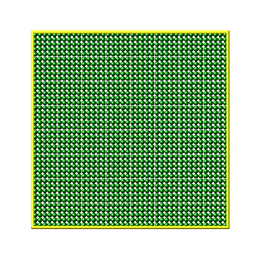
(a) (b)

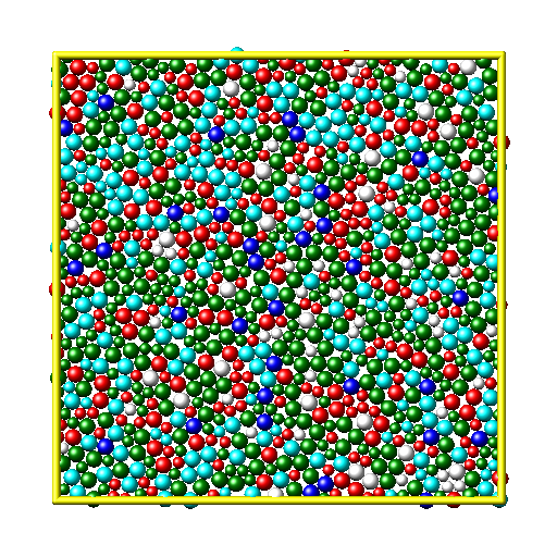
Figure 1: The two bidimensional surfaces studied in this work, each possessing a global average coordination number equal to four. (a) Perfect square lattice containing 1600, monodisperse sites. (b) Disordered configuration composed of a 50:50 mixture of 1000 sites of size ratio 1:4 (to suppress ordering during the configuration preparation protocol). Local site coordination is indicated by particle shading. Green equals a contact number of 4. The redder end of the spectrum represents lower number of nearest neighbors, whereas bluer shades are higher. Note: white/gray sites have zero contacts.

The implication of the term compensation is that any effect of variations in $E_{a}$ on the rate of the process, given by the Arrhenius equation $k=\nu\exp{\frac{E_{a}}{k_{B}T}}$, where $k_{B}$ is the Boltzmann constant and $T$ the temperature, are offset by variations in the prefactor $\nu$, in the same direction and with the same, or almost the same magnitude, such that $k$ remains relatively unchanged P. J. Estrup, E. F. Greene, M. J. Cardillo and J. C. Tully (1986); L. Liu and Q.-X. Guo (2001); Piguet (2014); J. B. Miller, H. R. Siddiqui, S. M. Gates, J. N. Russell Jr., J. T. Yates, J. C. Tully and M. J. Cardillo (1987); E. Tomkova and I. Stara (1998); A. Yelon, E. Sacher and W. Linert (2012); J. D. Dunitz (1995); E. Tomkova and I. Stara (1998); G. Gottstein and L.S. Shvindlerman (1998); A. Pan, T. Biswas, A. K. Rakshit and S. P. Moulik (2015).

The slope of Eq. 1 sometimes yields a temperature, called the compensation temperature $T_{c}$, as $\beta=\frac{1}{k_{B}T_{c}}$, at which a set of $\ln{k_{j}}$ vs. $\frac{1}{k_{B}T}$ plots are observed to cross and the rates $k_{j}$ acquire the same value $k_{j}=k_{o}$, and are said to become unaffected by external perturbations L. Liu and Q.-X. Guo (2001); A. Yelon, E. Sacher and W. Linert (2012); A. Pan, T. Biswas, A. K. Rakshit and S. P. Moulik (2015); B. V. L’vov and A. K. Galwey (2013); P. J. Barrie (2012a, b); K. F. Freed (2011). This convergence is called the isokinetic relation (IKR). The IKR is often mentioned interchangeably with the KCE A. Pan, T. Biswas, A. K. Rakshit and S. P. Moulik (2015); L. Liu and Q.-X. Guo (2001), perhaps because the occurrence of an IKR is often attributed to the parameters compensating each other at $T_{c}$ J. F. Douglas, J. Dudowicz and K. F. Freed (2009); L. Liu and Q.-X. Guo (2001), however the authors in L. Liu and Q.-X. Guo (2001) note that this mutual correspondence is only exact if the linear correlation coefficient between data points in Eq. 1 is $1$.

The KCE and IKR are generally identified as features of weak molecular interactions J. D. Dunitz (1995); Piguet (2014); Ford (2005) and, along with the closely related entropy-enthalpy compensation, have been reported in a wide range of phenomena in the physical, chemical, and biological sciences L. Liu and Q.-X. Guo (2001); K. F. Freed (2011), yet continue to be the subject of debate as to their existence and validity. Some authors claim that the KCE is a consequence of the exponential nature of the Arrhenius rate equation N. Koga and J. Šesták (1991); Cornish-Bowden (2002); P. J. Barrie (2012a). The observation of a strong linear correlation is commonly attributed to the parameters being extracted from the same temperature dependent data L. Liu and Q.-X. Guo (2001); P. J. Barrie (2012a); Cornish-Bowden (2002); J. Perez-Benito and M.Mulero-Raichs (2016), or deemed a consequence of experimental and/or statistical errors P. J. Barrie (2012a, b); J. Perez-Benito and M.Mulero-Raichs (2016).

In Ref. N. Zuniga-Hansen, L. E. Silbert and M. M. Calbi, 2018 we studied the kinetic compensation effect during the desorption of interacting and noninteracting adsorbates from an energetically homogeneous crystalline, square lattice surface. That previous study showed that the parameters exhibit a rather weak partial compensation effect in all regimes of interaction strength, because variations in $\nu$ are not strong enough to offset those in $E_{a}$. In addition, the observed IKR was found to be due to the system transitioning to a non-interacting regime, not because of a mutual offsetting between the Arrhenius parameters.

In the present work, we compare the results from the square lattice with those for the thermal desorption from a two dimensional disordered or amorphous surface. This is part of a systematic study where we implement a kinetic Monte Carlo scheme to numerically calculate the transient behavior of $E_{a}$ throughout the thermal desorption process of interacting and noninteracting adsorbates when different ‘experimental’ parameters are altered. The calculated data allow us to also obtain the transient variations in the prefactor, in order to quantify the level of compensation between $E_{a}$ and $\nu$. This approach differs from previous ones P. J. Estrup, E. F. Greene, M. J. Cardillo and J. C. Tully (1986); Piguet (2014); E. Tomkova and I. Stara (1998); J. D. Dunitz (1995); E. Tomkova and I. Stara (1998); E. B. Starikov and B. Norden (2007), in the sense that it does not part from the assumption that $E_{a}$ and $\ln{\nu}$ must satisfy the strong linear correlation in Eq. 1, nor preconceived functional forms based on it. In each set of results the net attractive interaction strength is the same, while the parameter that is being altered is the surface topology. These results also allow for an overview of the kinetics of desorption from amorphous surfaces, which constitutes an important problem, since disorder is present in many realistic systems, and exact functional forms can be difficult to obtain J. Talbot, G. Tarjus and P. Viot (2007, 2008).

II Methodology

We use the kinetic Monte Carlo algorithm Voter (2007) to simulate the thermal desorption of interacting and noninteracting, quasispherical adsorbates from the bidimensional surface configurations shown in Fig. 1. This study focuses on the comparison and contrast between the two particular surfaces: a two-dimensional square lattice and a two-dimensional disordered surface. The main distinction between them is the distribution of site coordinations. For the square lattice (Fig. 1(a)) each site has exactly four neighbors. Therefore, the global average coordination number for the ‘ordered’ square lattice is also precisely four, $z_{O}=4$. Whereas, for the disordered configuration (Fig. 1(b)), the local site coordination number is not constant such that there are varying numbers of nearest neighbors from site to site, spanning 0 to 6. This variation in site coordination is indicated by the particle shading in Fig. 1. However, the disordered surface has been prepared such that it’s average coordination number matches that of the square lattice, i.e. $z_{D}=4$. The disordered surface is fully representative of a realistic disordered system, such as a connected layer of sand grains or an amorphous, glassy substrate Coniglio et al. (2004).

For this study, the lattices are energetically homogeneous, with binding energy $E_{i}=E_{b}=100$, in units where $k_{B}=1$. The index indicates the $i^{th}$ site on the surface. Lateral adsorbate-adsorbate interactions are added as a parameter $\epsilon$, which is calculated as a percentage of $E_{b}$. The interaction strengths employed in this study are $0\%$, $10\%$, $50\%$ and $90\%$ of the binding energy.

To track the desorption process, the kinetic Monte Carlo algorithm follows a series of steps. First, initial conditions are specified. This includes binding and interaction energies ($E_{b}$ and $\epsilon$, respectively), initial temperature $T_{0}$ (which is modified depending on $\epsilon$), step size for temperature increase $\gamma$, as $T=T_{0}+\gamma t$, and initial coverage, here set at monolayer ($100\%$) for all cases. During the second step the algorithm calculates the number of occupied nearest neighbors per site, as well as site energies in order to determine transition probabilities. These are calculated as $W_{i}=e^{\beta E_{i}}$, where $E_{i}$ is the energy barrier of the $i^{th}$ adsorption site, given by

$$E_{i}=E_{b}+\sum_{m=1}^{z_{i}}n_{im}\epsilon,$$

where each site $i$ picks up an energy contribution from its $z_{i}$ nearest occupied neighbors. Thus, $n_{im}=1$ when a neighbor site is occupied, and is zero if empty.

Next, a random number $x_{1}$ between $0$ and $1$ is generated, to select an allowable transition (desorption or diffusion to a neighboring available site). The selected change of state is that with the largest probability, which satisfies the following inequality

$$\frac{1}{W}\sum_{j=1}^{k-1}W_{ij}<x_{1}<\frac{1}{W}\sum_{j=1}^{k}W_{ij},$$

where $W_{ij}=e^{\beta(E_{i}-E_{j})}$ is the transition probability from state $i$ to state $j$. The sum $W$ of all probabilities is over all $k$ allowed transitions per site $i$. Lower probability transitions can still take place, to allow the system to evolve freely, and avoid forcing it to follow a particular path. After every transition, the time variable $t$ increases by a fractional amount determined by a second random number. Temperature increases according to the step size $\gamma$, here set to $1$ degree per unit of time. The average site occupancy and energy are recorded at every iteration, and the process is repeated until all the particles have desorbed. The results are obtained as an (ensemble) average over many independent runs.

The data analysis is done with the Polanyi-Wigner equation for desorption,

$$-\dot{\theta}=\theta^{n}\nu\exp{\frac{-E_{a}}{k_{B}T}}$$ (2)

where $\theta$ is the fractional coverage and $\dot{\theta}$ its time derivative, $n$ is the order of the process, which is set to $n=1$ for reversible thermal desorption. It is worth pointing out that Eq. 2 can only be fit exactly in the noninteracting regime, where $E_{a}$ and $\nu$ remain constant, or if their functional forms are known. In the present work the numerical data for $E_{a}$, along with $\dot{\theta}$ are used to extract the nonconstant preexponential factor.

III RESULTS

III.1 Rates of desorption and Arrhenius plots

The first series of results consists of a comparison between desorption rate curves, and corresponding Arrhenius plots from both surfaces. In each set the interaction strength is the same, and the parameter that is being altered is the surface morphology. The values of the interaction energy $\epsilon$ for the data sets presented in this series are $0\%$, $10\%$, $50\%$ and $90\%$ of the binding energy, $E_{b}=100$. (In the proceeding figures we plot the magnitude of $E_{a}$, as the activation energy itself is negative.)

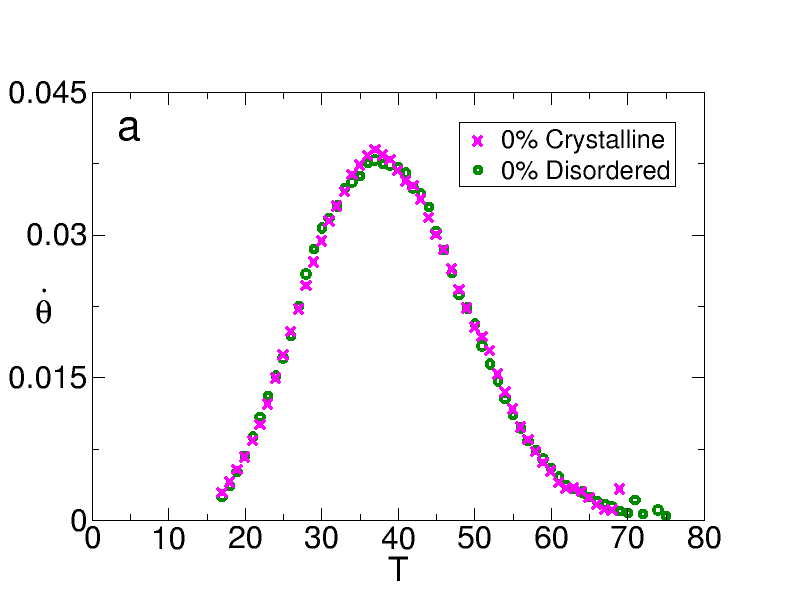
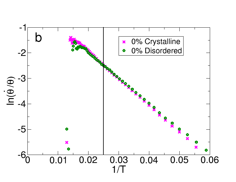
Figure 2: Thermal desorption rates from both the crystalline (ordered) and disordered surfaces for noninteracting species. (a) Desorption rate $\dot{\theta}$ and (b) corresponding Arrhenius plot. The solid black line in (b) indicates the crossing temperature of the Arrhenius plots.

In the non-interacting regime (Fig. 2) the desorption rate curves from both surfaces in Fig. 2(a) exhibit very little differences, since the curves almost overlap completely for the entire process. The corresponding Arrhenius plots in Fig. 2(b) also exhibit significant overlap, nevertheless, a small gap at low temperatures can be seen upon closer inspection. The plots come closer together as $T$ increases, and cross at approximately $T=40$ (or $\frac{1}{T}=0.025$). This could be an isokinetic relation in the traditional sense, however, it cannot be associated with a compensation effect, since the activation energy is constant and cannot influence the preexponential factor. Nevertheless, the rates, $k\equiv\frac{\dot{\theta}}{\theta}$, for both surfaces acquire close values at $T=40$, where their ratio (ordered / disordered) is $k_{O}/k_{D}\approx 0.985$.

A thermodynamic interpretation of the Arrhenius parameters states that the prefactor has an entropy component, $e^{\frac{\Delta S}{k_{B}}}$, where $\Delta S$ is the change in the entropy, and a frequency component, $\kappa$ K. Sharp (2001); G. Gottstein and L.S. Shvindlerman (1998); Piguet (2014), of attempted events, in this case of desorption events. Sometimes an additional factor $\rho$ is considered, which corresponds to geometric constants of the system in question G. Gottstein and L.S. Shvindlerman (1998).

In the non interacting regime the observed differences can be attributed to the frequency of desorption events. This is because the disordered surface has sites with varying numbers of nearest neighbors, $0\leq z_{i}\leq 6$. Sites with $z_{i}=0$, the ‘rattlers’, have no nearest neighbors, and thus a particle initially located there is only allowed to desorb. This is therefore the initial step in the desorption process for the disordered surface. For sites with larger coordination number, connectivity to neighboring sites allows particles to diffuse to a nearest available location. This tends to be the preferred transition at lower temperatures, and causes particles to linger on the surface slightly longer. In addition, sites with larger values of $z_{i}$ are more accessible to particles that remain on the surface, making their reoccupation easier, which also contributes to their coverage decreasing at a slower pace. There is also a decrease in configurational entropy arising from the various coordination numbers. Once particles desorb from rattler sites there is no probabilty for reoccupation, since, in this study, we exclude readsorption, mimicking the process whereby desorbed particles are extracted from the chamber in an experiment. Additionally, sites with lower values of $z_{i}$ are also less accessible once unoccupied than those with more nearest neighbors. This limits the number of ways that the remaining particles can be distributed among the available locations in the amorphous configuration. These factors add complexity to the desorption process, as they result in multiple desorption rates. In this particular configuration they produce a slightly different value of $\ln{k}\equiv\ln\left(\frac{\dot{\theta}}{\theta}\right)$ from that in the crystal at low $T$, since the overall curve is the average of all those contributions.

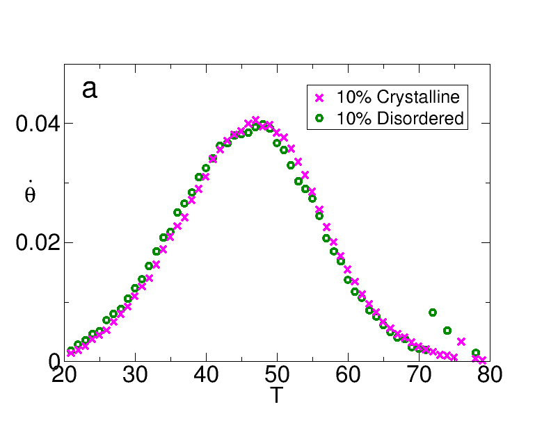
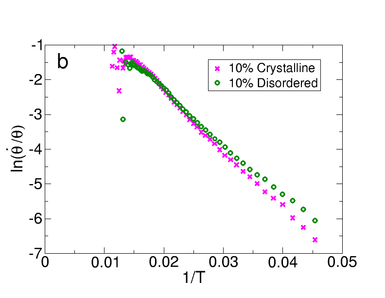
Figure 3: Thermal desorption rates from the crystal and the disordered surfaces (a), and corresponding Arrhenius plots (b), at $10\%$ interaction strengh. The Arrhenius plots in this regime exhibit the behavior associated with an isokinetic relation (IKR). The crossing temperature is visually estimated at $T\approx 47$. The KCE is associated with weak molecular interactions, and the fairly linear Arrhenius plots allow the extraction of apparently constant values of $E_{a}$ and $\ln{\nu}$.

Even at only $10\%$ interaction strength, differences in the desorption rates become more evident, as shown in Fig. 3(a), but nevertheless remain small. These differences should be expected, since lateral interactions, combined with varying site values of $z_{i}$ for the disordered surface, add energetic heterogeneity to the lattice, so that differences between sites are enhanced.

The corresponding Arrhenius plots in Fig. 3(b) also exhibit more noticeable differences. The initial gap between them is larger, and they eventually converge and exhibit an IKR. For this data set, the temperature of greatest overlap between the ordered and disordered surfaces, shown in Fig. 3(b), occurs at $T\approx 47$, at which point the Arrhenius parameters almost match exactly, where the fractional surface coverage reaches $50\%$. Even though the parameters are numerically close, this contrasts with the results of Ref. N. Zuniga-Hansen, L. E. Silbert and M. M. Calbi (2018), where the overlap occurred when the system transitioned to the non-interacting regime. Here, at the crossing point, lateral interactions still have some effect, and it appears that the reason for the convergence is that the effective average coordination number $z_{i}$ occupancy per site becomes almost the same in both surfaces, at $z\approx 1$ (as seen in the values of $E_{a}$). This presents a different scenario where an IKR is observed, but one which also precludes the occurrence of complete compensation between $E_{a}$ and $\ln{\nu}$.

The IKR observed here, as well as that in Ref. N. Zuniga-Hansen, L. E. Silbert and M. M. Calbi (2018), for this same weak interaction regime ($\leq 10\%$), which is accompanied by a strong linear correlation that fits Eq. 1, shows why these phenomena are usually ascribed to weak molecular interactions K. Sharp (2001); J. D. Chodera and D. L. Mobley (2013); Ford (2005); Piguet (2014).

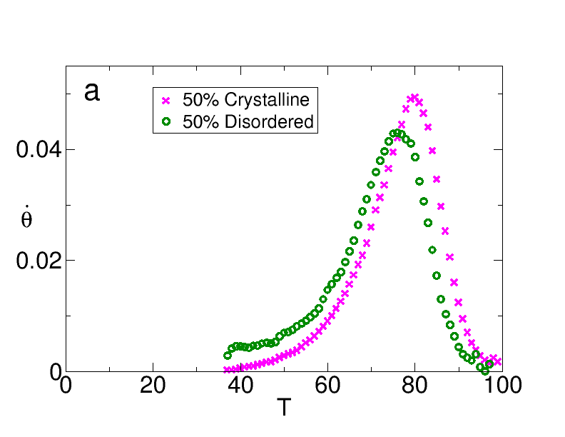
Figure 4: Comparison of thermal desorption rates from the crystal and the amorphous surface at (a) $50\%$ and (b) $90\%$ interaction strength. The desorption rate increases in the amorphous surface where multiple rates arise due to varying coordination numbers $z_{i}$ from site to site.

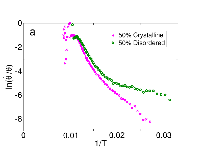
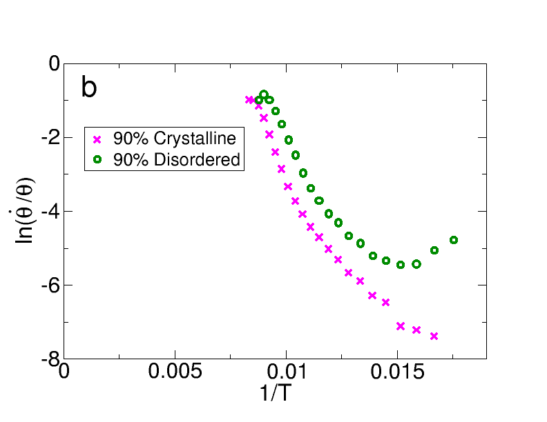
Figure 5: Comparison between Arrhenius plots from the crystal and the amorphous surface, at (a) $50\%$ and (b) $90\%$ interaction strength. In the disordered configuration the curvature of the Arrhenius plots becomes more pronounced as interaction strength increases. The plots appear to come together at high values of the temperature where both surfaces are almost empty.

In the $50\%$ and $90\%$ interaction strength regimes, the desorption rates in Figs. 4(a) and (b), respectively exhibit even more pronounced differences. The rate of desorption is visibly faster in the disordered surface and peaks at a lower temperature There is also a visible ‘tail’ on the left end of the thermal desorption peak at $90\%$ interaction strength (see Fig. 4(b)) from the disordered surface. This feature does not appear at $50\%$ interaction strength, but the thermal desorption peak does not start at $0$ on the abscissa. The corresponding Arrhenius plots in Figs. 5(a) and (b) exhibit sub Arrhenius type behavior V. H.C. Silva, V. Aquilanti, H. C. B. de Oliveira and K. C. Mundim (2013), i.e. a concave curvature, signature of a variable energy of activation S. Vyazokin (2016), but the curvature becomes significantly more pronounced for the disordered configuration.

III.2 Kinetics of desorption from an amorphous surface: an overview

The shape of the Arrhenius plot is determined by the Arrhenius parameters $E_{a}$ and $\ln{\nu}$, however, their transient variations, as well as some of the features observed in the desorption rate peaks and Arrhenius plots in the amorphous configuration, can be explained by looking at the individual contributions from each group of sites, with specific $z_{i}$ values, to the overall rates of desorption, as an initial overview to a more extensive study on the kinetics of desorption from two dimensional amorphous lattices.

The results in this section are in order of increasing interaction strength, from lowest to highest, starting with the non-interacting regime in Fig. 6, where Fig. 6(a) shows the rates of coverage decrease for the overall surface (solid black line), and the contributions from each group of sites (symbols), classified according to their coordination number $z_{i}$. Figure 6(b) shows a magnified view of site contributions alone.

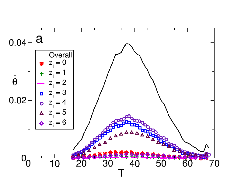
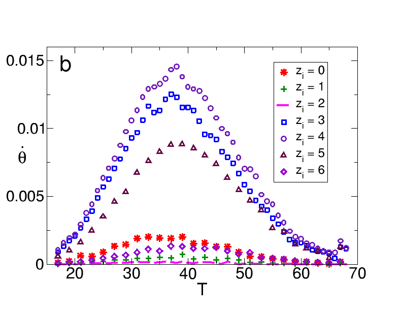
Figure 6: Desorption rates as function of temperature at $0\%$ interaction strength. (a) Overall rate, and contributions for each group of sites, classified according to their coordination number $z_{i}$. (b) Magnified view of the site contributions, the peak from sites with $z_{i}=0$ reaches a maximum at a slightly lower temperature than other sites, indicating faster desorption.

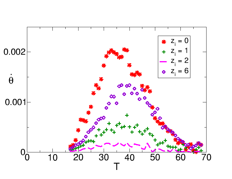
Figure 7: Desorption rates as function of temperature at $0\%$ interaction strength for sites with $z_{i}=0,~{}1,~{}2,~{}6$. Desorption from sites with $z_{i}=0$ occurs at a faster rate than others, whereas desorption from sites with $z_{i}=6$ occurs last. The desorption rate is governed mainly by a greater probability for diffusion, as the number of nearest neighbors $z_{i}$ increases.

In Fig. 6(a) the peak for sites with $z_{i}=0$ reaches a maximum at a slightly lower temperature than the rest, as it shifts leftward with respect to the others, this is easier to see in the zoomed-in plot of Fig. 7. In Fig. 6(b) it can also be seen that there are very mild differences in the peak temperatures for sites with $3\leq z_{i}\leq 5$, as the $z_{i}=5$ peak is shifted slightly rightward, indicating a slightly slower desorption rate. The $z_{i}=6$ sites have the slowest desorption rate, since the corresponding peak is shifted toward high temperature with respect to the rest, this is easier to see in Fig. 7. As mentioned before, the rates vary from site to site only because of varying site coordination, which results in some sites having ‘options’ to diffuse to an available nearest neighbor, slowing down desorption from those locations. The small differences between non-interacting Arrhenius plots at low $T$ in Fig. 2(b) are likely caused by the fast initial desorption from sites with $z_{i}=0$, but the differences are not so prominent when the binding energies are the same at all sites. The various rates result in varying frequencies of desorption events, and, although very mildly for this system, this affects the frequency of desorption events of the preexponential factor $\nu$ in a way that is independent of molecular interactions.

There is some irony in how the intrinsic disorder of the amorphous surface reduces the same randomness in the desorption process that makes this regime trivial in the crystalline lattice. A different site distribution would perhaps accentuate differences and might cause the Polanyi-Wigner equation of desorption to fail to model the overall desorption rate J. Talbot, G. Tarjus and P. Viot (2007, 2008); N. Zuniga-Hansen and M. M. Calbi (2012).

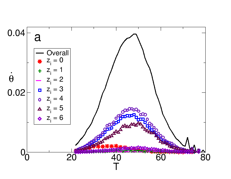
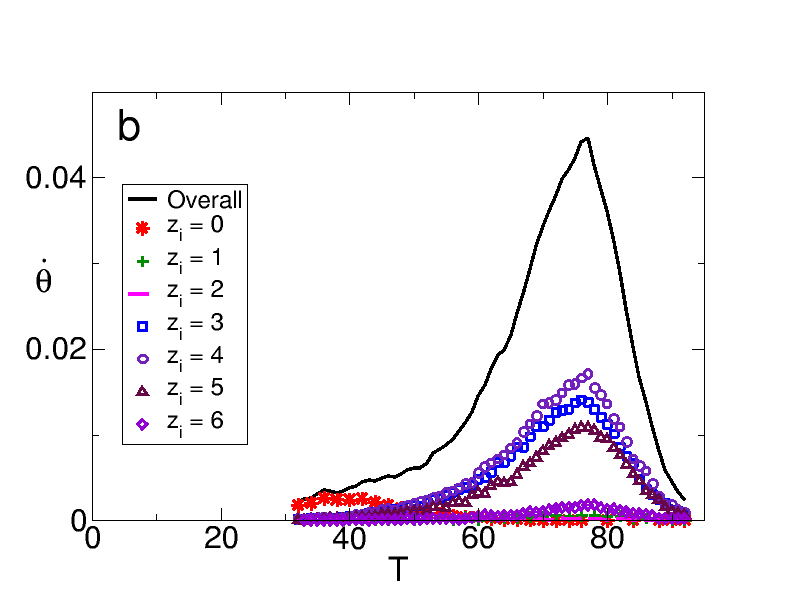
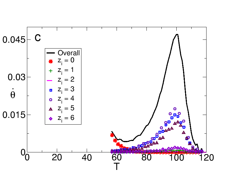
Figure 8: Desorption rates as function of temperature at (a) $10\%$ (b) $50\%$ and (c) $90\%$ interaction strengths. The overall rate is the solid black line. Site contributions are classified according to their coordination number $z_{i}$, and plotted in symbols.

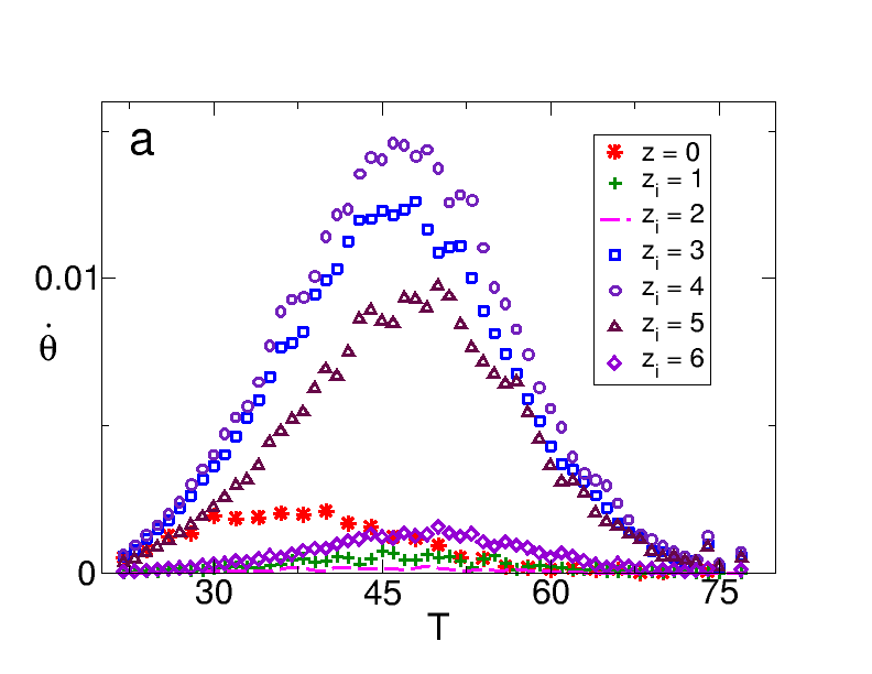
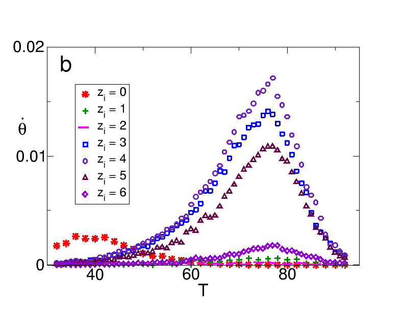
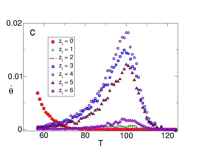
Figure 9: Magnified view of site contributions at (a) $10\%$, (b) $50\%$ and (c) $90\%$ interaction strengths. The first step in the process is fast desorption from sites with $z_{i}=0$ nearest neighbors. The rest of the peaks shift rightward with respect to the rattler one, indicating slower desorption rates. Note that the temperature axis does not start at $0$ to provide a magnified view.

In the interacting regime adsorption sites have the additional energetic contribution of attractive lateral interactions. This increases the effective desorption barrier to be overcome by particles, which also depends on the coordination number of the site at which they are located, and also results in an energetic heterogeneity that yields various desorption rates, as seen in Fig. 8. Sites with $z_{i}=6$ naturally provide the largest desorption barrier.

In Figs. 8(a), (b) and (c), the desorption rate peak for $z_{i}=0$ remains to the left of the rest, but changes in shape. At $10\%$ and $50\%$ interaction strengths (Figs. 8(a) and (b), repsectively) the $z_{i}=0$ peaks retain the typical thermal desorption shape. However, for $\epsilon=0.5E_{b}$ its leftmost end does not start at $0$ on the abscissa, which is the reason why the overall rate curve in Fig. 8(b) does not start at $0$ either. At $90\%$ interaction strength (Fig. 8(c)) the $z_{i}=0$ peak is seen to produce the lefmost ‘tail’ on the left end of the overall rate. In this interaction regime this initial step takes place very fast, like flash desorption.

These features can be seen more clearly in Figs. 9(a), (b) and (c), where the magnified picture of site contributions in the $10\%$, $50\%$ and $90\%$ interaction regime, respectively, are shown.

The differences in the shapes of the $z_{i}=0$ peaks can be attributed to the initial temperature $T_{0}$ of the simulation run, which, for purposes of comparison, was selected to match that of the same interaction strength regime of the crystal, given that the Arrhenius plots are constructed as a function of $\frac{1}{T}$.

If $T_{0}$ is set to the same low value for all regimes of interaction strength in the amorphous surface, the $z_{i}=0$ desorption rate peak spans the same temperature range and has the same typical shape in all cases. This can be seen in Fig. 10, where only the $z_{i}=0$ and overall desorption rates are shown. This demonstrates that this desorption rate depends solely on $T_{0}$, and is independent of lateral interactions.

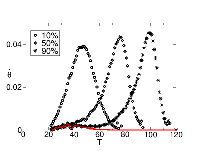
Figure 10: Overall rates of desorption for $10\%$, $50\%$ and $90\%$ interaction strength (symbols) and rates of desorption from rattler sites (red lines). The rates of desorption from rattler sites depend only on initial temperature. The red curves on the left overlap when a common value of $T_{0}$ is used for all desorption runs. This feature, in addition to faster rates from sites with $z_{i}<4$, yields an overall faster rate of desorption in the amorphous surface.

The transient variations in the Arrhenius parameters throughout the desorption process will be explored next.

III.3 Activation Energy

As part of a systematic study of the kinetic compensation effect in thermal desorption, this section presents the numerically calculated transient variations in the energy of activation per site, per iteration, as a function of coverage $\theta$. Site contributions to the overall $E_{a}$ curves were also calculated. As previously mentioned, this study is intended to explore how a change in an ‘experimental’ parameter (in this case the surface configuration) may result in a KCE, an IKR, or both.

Figure 11 shows a comparison between the numerically calculated $E_{a}$ curves throughout the desorption process from the crystalline (lines) and the amorphous surface (symbols), for all regimes of interaction strength studied here.

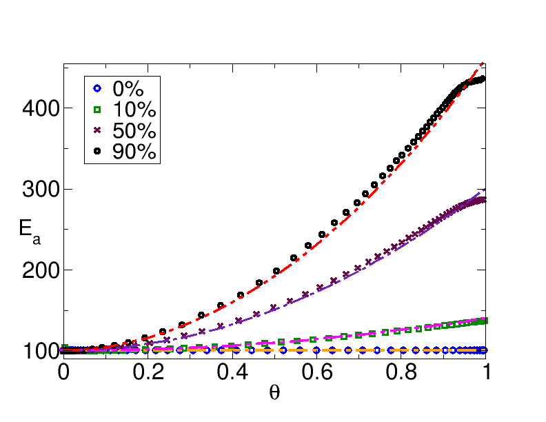
Figure 11: Effective activation energy $E_{a}$ as a function of coverage $\theta$ at $0\%$, $10\%$, $50\%$ and $90\%$ interaction strength. Comparison between the crystalline and disordered surfaces. $E_{a}$ for the disordered surface exhibtis the same functional form as that of the crystal, except for a small initial difference in the presence of interactions, more visible at $50\%$ and $90\%$ interaction strengths.

At $0\%$ interaction strength, $E_{a}$ remains constant through the entire process, as expected, and all site contributions, shown in Fig. 12, remain constant as well.

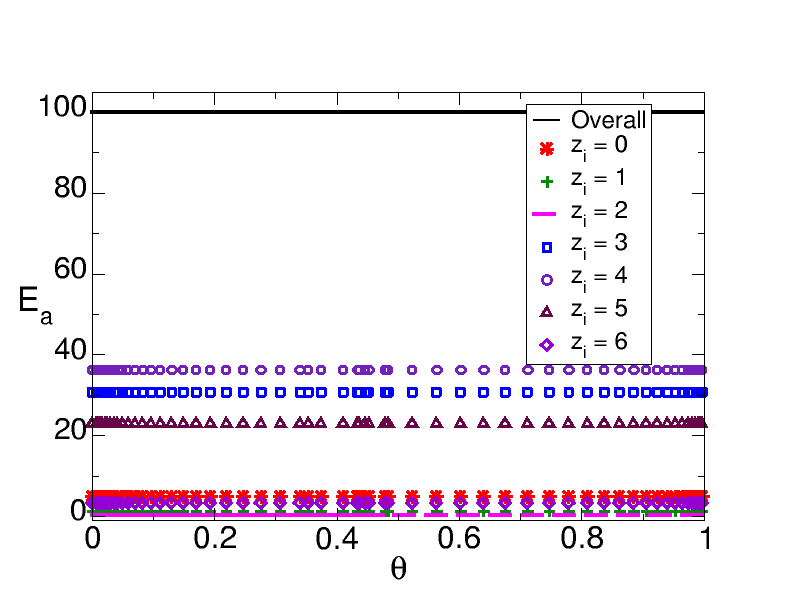
Figure 12: Activation energy $E_{a}$, per site as function of coverage $\theta$, for the amorphous surface, at $0\%$ lateral interaction strength. In this regime all site contributions ti $E_{a}$ remain constant.

Fig. 11 also shows that in the interacting regime the behavior of $E_{a}$ from the disordered surface did not deviate much from the behavior observed for the crystal in N. Zuniga-Hansen, L. E. Silbert and M. M. Calbi (2018), except for an initial numerical difference, followed by a brief ‘stagnation’ at the initial stage of the desorption process (at low $T$ and high coverage), where $E_{a}$ in the amorphous surface briefly decreases from its largest magnitude at a slower pace, before regressing to the behavior observed in the crystal. These initial differences are more visible at $50\%$ and $90\%$ interaction strengths, but also occur at $10\%$ interaction strength, and can be seen in the zoomed-in picture in Fig. 13.

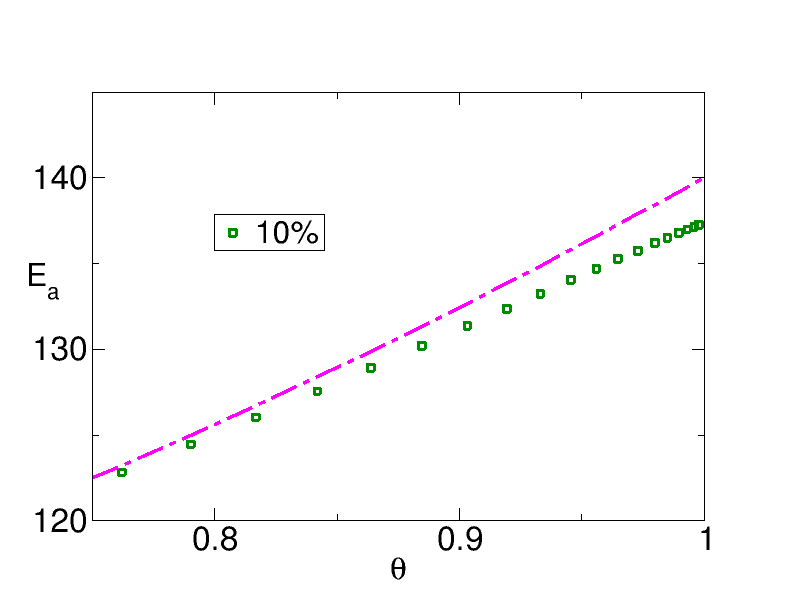
Figure 13: Magnified view of the initial stages of the variation of $E_{a}$ as function of coverage $\theta$, at $10\%$ interaction strength. The initial difference between $E_{a}$ curves is also observed in this interaction regime.

The initial numerical difference arises because the effective average coordination number $z_{i}$ per site at monolayer coverage is $3.87$ for the amorphous surface, and $4$ for the crystal. The initial ‘stagnation’ occurs because rattler desorption dominates this initial stage, with a net energetic contribution to the overall $E_{a}$ curve of $0$. And, while this step takes place, desorption from sites with $z_{i}=3$ to $z_{i}=6$ occurs more slowly, which is why the overall $E_{a}$ curve also decreases more slowly. This is not very evident in Fig. 14, but can be seen in Figs. 15(a) and (b), where site contributions to the overall $E_{a}$ curve at every recorded stage of the process are plotted.

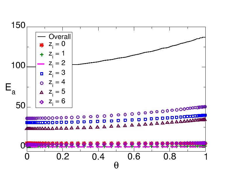
Figure 14: Activation energy per site as function of coverage in the amorphous surface at $10\%$ interaction strength. In the presence of lateral interactions only the contribution from sites with $z_{i}=0$ (red stars) remains constant, while site contributions for $z_{i}>0$ (symbols) vary in a similar fashion as the overall curve (black solid line).

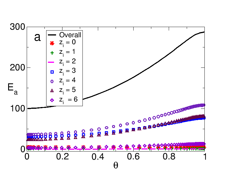
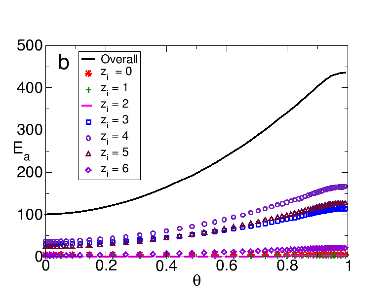
Figure 15: Activation energy per site as function of $\theta$ in the amorphous surface at (a) $50\%$ and (b) $90\%$ interaction strengths. Site contributions (symbols) show that $E_{a}$ decreases from its initial magnitude more slowly as $z_{i}$ increases. The initial ‘stagnation’ is produced by slower decrease from the initial $E_{a}$ magnitude for sites with $3\leq z_{i}\leq 5$. The rattler contribution remains constant in all regimes of interaction strength.

In Figs. 15(a) and (b), the $z_{i}=3$ to $z_{i}=5$ curves have the most visible effect on the shape of the overall $E_{a}$ curve. The $z_{i}=1$ and $z_{i}=2$ curves are not mentioned, this is because there is a very small number of these sites, and their net contribution to the overall is rather negligible. For $z_{i}=6$ the corresponding $E_{a}$ curve changes even more sluggishly than the rest, but a smaller number of these sites compared to those for $z_{i}=3$ to $z_{i}=5$ causes their net effect to average out.

III.4 Preexponential factor

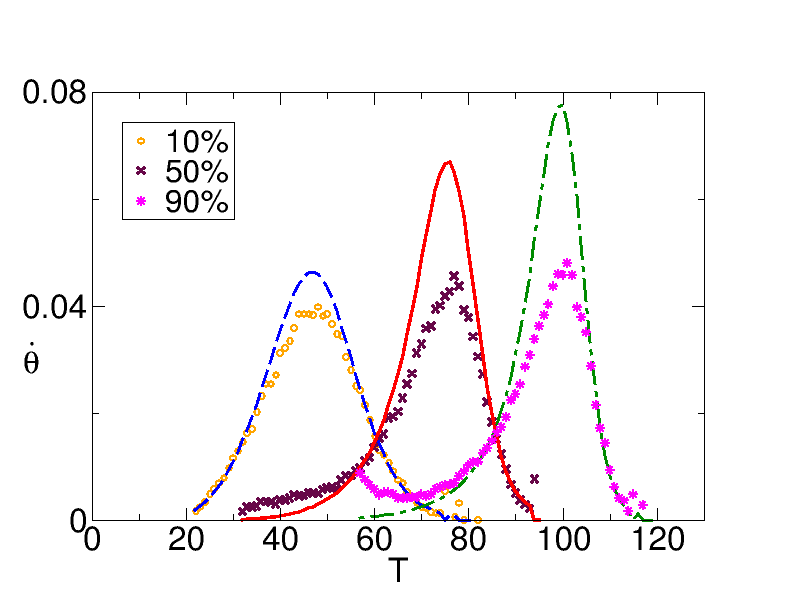
Figure 16: Comparison of rates of desorption in the amorphous surface. The solid lines represent the peaks calculated with the Polanyi-Wigner equation, Eq. 2, using the numerical data for $E_{a}$, $\theta$, and $T$, and setting $\nu=1$. The symbols represent the time derivative taken directly from the coverage data. The difference between the peaks indicates a compensation effect due to variations in the prefactor.

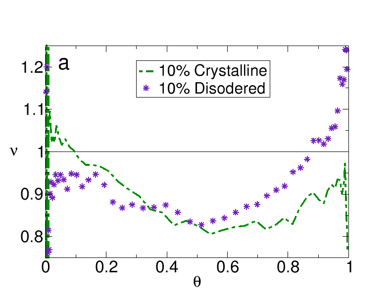
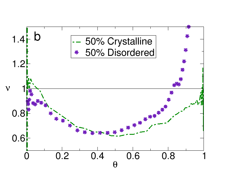
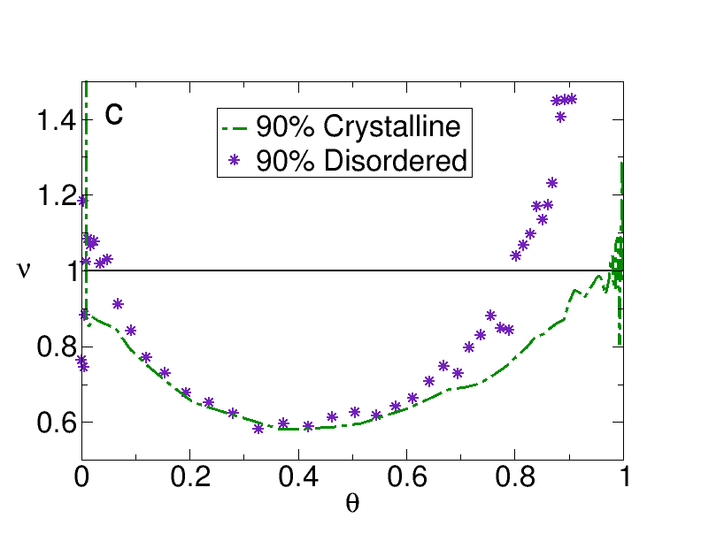
Figure 17: Preexponential factor as a function of coverage for $10\%$, $50\%$, and $90\%$ interaction strength in increasing order from top to bottom. The prefactor $\nu$ from the amorphous configuration exhibits very large variations, above its standard value of $1$, at high coverage values. At about $80\%$ fractional surface coverage, $\nu$ for the amorphous surface drops below $1$ and rescinds to the behavior observed for the crystal, where the decrease is likely originated by a decrease in the frequency of desorption events and configurational entropy.

The preexponential factor in the amorphous surface is calculated by dividing two desorption rate peaks. One is obtained directly from the time derivative $\dot{\theta}$ of the surface coverage decrease data, the result is represented by symbols in Fig. 16, and the analytically calculated rate, using Eq. 2 for order $1$, with the numerical data for $E_{a}$, $\theta$ and $T$, and setting $\nu=1$, represented by straight lines in Fig. 16, in the same manner as was done for the crystal in N. Zuniga-Hansen, L. E. Silbert and M. M. Calbi (2018). The differences between the rates indicate that there is some amount of compensation, which is greater at the peak temperature. Also, the prefactor contribution is what generates the leftmost ‘tail’ at $90\%$ interaction strength, and it is also the reason why the overall peak does not start at $0$ on the abscissa at $50\%$ interaction energy.

The calculated prefactors for each interaction strength regime are plotted in Fig. 17, and overlayed with the results from the crystal from N. Zuniga-Hansen, L. E. Silbert and M. M. Calbi (2018) for comparison. In Figs. 17(a), (b) and (c) it is seen that, in the interacting regime, $\nu$ from the amorphous configuration exhibits large variations at the beginning of the desorption process, and then drops below $1$ at around $80\%$ fractional surface coverage. At this point, the behavior of $\nu$ closely resembles that of the prefactor in the crystal. The large variations at high coverage values show the fast initial desorption from rattler sites, this mostly affects the frequency component of $\nu$, as it is a result of the increase in the frequency of desorption events. When $\nu$ drops from unity, there is a slowdown in the number of those same events, due to island formation S. Gunther, T.O. Mentes, M.A. Nino, A. Locatelli, S. Bocklein and J. Wintterlin (2014) and increased effective desorption barriers. This clustering also causes a decrease in configurational entropy, but in the amorphous surface there is the additional factor of sites with $z_{i}=0$ being unavailable for reoccupation after particles desorb, and also that the different $z_{i}$ values from site to site make some locations easier to reoccupy than others. The latter effect does not seem too pronounced in this configuration, since the variations in $\nu$ are very close to those in the crystal. Perhaps this is due to all sites having the same binding energy. It may become more prominent for a different site distribution, or if the lattice is energetically heterogeneous N. Zuniga-Hansen and M. M. Calbi (2012).

III.5 Kinetic compensation effect for the amorphous surface

Here the contributions of $E_{a}$ and $\nu$ to the overall Arrhenius plots for the disordered surface are quantified. This is done by directly comparing the two sides of the natural logarithm of the Arrhenius equation, which gives the following:

$$\ln{k}=\frac{-E_{a}}{T}+\ln{\nu}$$ (3)

All terms in Eq. 3 in are calculated with the numerical data in the previous sections, and plotted as function of $\frac{1}{T}$. Here $k=-\frac{\dot{\theta}}{\theta}$. The first set of results correspond to the non-interacting regime (Fig. 18).

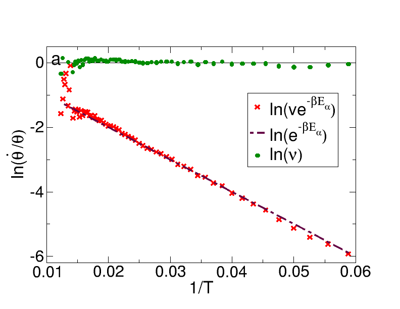
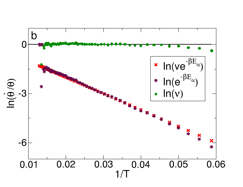
Figure 18: Arrhenius plot (red stars) and separate contributions from $E_{a}$ (purple dashed line) and $\nu$ (green dots) at $0\%$ interaction strength for (a) the amorphous surface, and (b) the crystal. The $E_{a}$ contribution almost overlaps completely with the Arrhenius plot in this regime, except for a portion at the beginning of the desorption process, which happens when the prefactor slightly drops below the $0$ axis in the figure.

In the absence of lateral interactions, the $E_{a}$ contribution almost completely overlaps with the overall Arrhenius plot, but there are some small differences at the beginning of the process, where there appears to be a slight drop of the $\ln{\nu}$ plot from $0$. This can be seen with the reference axis added in Fig. 18(a). This may be purely numerical, therefore the same results for the crystal are plotted in Fig. 18(b) for comparison. A drop is observed here too, however it is more pronounced. The drop could also be caused by a brief initial slowdown in the frequency of desorption attempts due to low initial temperature.

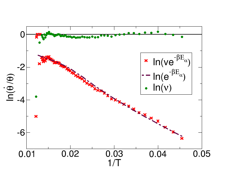
Figure 19: Arrhenius plot (red stars), separate contributions from $E_{a}$ (purple dashed line), and $\nu$ (green dots) at $10\%$ interaction strength. The $E_{a}$ contribution almost completely overlaps with the Arrhenius plot in this regime, but there are some differences, showing a small level of partial compensation due to $\ln{\nu}$. The KCE and IKR are usually attributed to weak molecular interactions, where the Arrhenius plots can be fitted to a straight line.

At $10\%$ interaction strength, in Fig. 19, the Arrhenius plot is very mildly curved, but can still be fit to a straight line. The prefactor contribution $\ln{\nu}$ shows small variations that are consistent with its transient behavior observed in Fig. 17(a): first there is a variation in the opposite direction of $E_{a}$, where $\nu$ acquires very large values, and after this a small drop from zero, similar to that observed in the crystal. These features are not so visible here, but the trend is easier to see as the interaction strength parameter $\epsilon$ is increased.

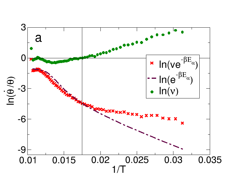
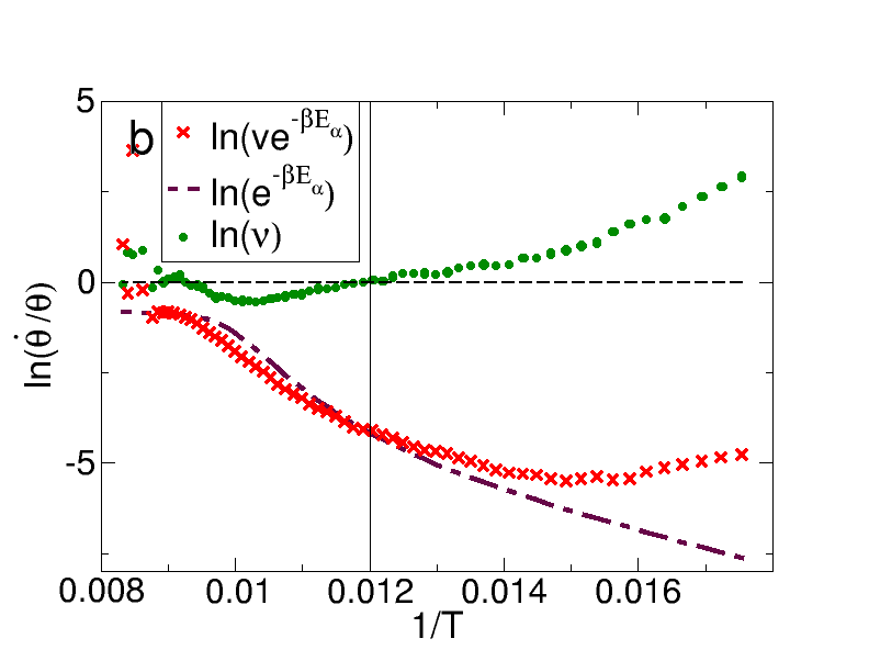
Figure 20: Arrhenius plot (red stars), separate contributions from $E_{a}$ (purple dashed line), and $\nu$ (green dots) at (a) $50\%$ and (b) $90\%$ interaction strength. There is a large difference between the $E_{a}$ contribution and the overall Arrhenius plot, because of the large initial variation in the preexponential factor. This $\ln{\nu}$ contribution varies in the opposite direction of $E_{a}$, and mitigates the effect of the enhanced effective desorption barrier due to interactions, but is independent of $E_{a}$. After this step $\nu$ weakly compensates for changes in $E_{a}$.

In the $50\%$ and $90\%$ regimes (Figs. 20(a) and (b), respectively), it can be seen that the large initial variation in the prefactor (Figs. 17(b) and (c)) generates the increased curvature of the Arrhenius plot, while the $E_{a}$ contribution by itself results in an Arrhenius plot that is slightly curved, a signature of the variable energy of activation S. Vyazokin (2016), and closely resembles the $E_{a}$ contributions and Arrhenius plots observed for the crystal N. Zuniga-Hansen, L. E. Silbert and M. M. Calbi (2018).

Whenever there is a decrease in $E_{a}$ (i.e., more negative and therefore corresponds to a stronger binding) that results in a decrease in configurational entropy, it is said that there is a compensation effect L. Liu and Q.-X. Guo (2001); Piguet (2014). This implies that the parameters move in the same direction and offset each other. If the parameters move in the opposite direction, for example if $E_{a}$ becomes less negative for repulsive interactions, the configurational entropy would still decrease, in this case mainly because of site exclusion. Then this is referred to as the less explored anti compensation effect, where in principle the parameters would vary in the opposite direction Piguet (2014). The fast initial desorption resembles the effect of a net repulsive interaction, even though repulsive interactions are not included explicitly in this study. Nevertheless, it mitigates the slowdown in frequency of desorption events due to the enhanced desorption barriers, so it is somehow compensating for these changes in the opposite direction. However, the fast initial desorption is independent of lateral interactions and, as seen in Fig. 10 it depends only on the initial temperature, and raises the question of whether this can be characterized as any type of compensatory behavior at all, given the lack mutual dependence. Nevertheless, this factor plays a role in determining the overall rate, and would be omitted if the functional characterization of $\nu$ is done based on the a priori assumption of complete compensation between $E_{a}$ and $\ln{\nu}$ to satisfy Eq. 1. A similar point is made in ref. J. D. Chodera and D. L. Mobley (2013).

Many authors question the validity of a strong linear correlation on the basis of the percentage error with which the parameters can be obtained from experimental data J. Perez-Benito and M.Mulero-Raichs (2016); P. J. Barrie (2012a); Cornish-Bowden (2002); J. D. Chodera and D. L. Mobley (2013). However, given that the breakdown of the contributions in this section show that, at least in this system, no complete compensation occurs, it also seems reasonable to ask, if the slope of Eq. 1 does not match the crossing temperature, what is the information that a strong linear correlation between the parameters provides? Perhaps it is a semi-empirical relation between apparent Arrhenius parameters which could be useful to characterize the effects of experimental changes in activated processes, much how apparent Arrhenius parameters allow for the semi-empirical characterization of rates P. J. Barrie, C. A. Pittas, M. J. Mitchell and D. I. Wilson (2011); Agrawal (1986).

IV Conclusions

In summary, attemping to characterize $\nu$ purely as a function of $E_{a}$, and vice versa, in order to force the parameters to mutually compensate each other and fit the linear correlation in Eq. 1 may omit important factors that determine the overall rate of a process. For the amorphous configuration in this study, the most prominent factor is the fast desorption from sites with $0$ nearest neighbors. This initial step is independent of lateral interactions and yields variations in $\nu$ in the opposite direction to those in $E_{a}$. This raises the question of whether this can be characterized as a compensation effect, yet the increase in the frequency of desorption events mitigates the effect of a larger potential barrier to be overcome by adsorbates in the presence of attractive interactions. After the initial desorption step, $\nu$ is observed to partially compensate for changes in $E_{a}$, in a similar manner to that observed in N. Zuniga-Hansen, L. E. Silbert and M. M. Calbi (2018). This type of weak compensation is also favored by other authors L. Liu and Q.-X. Guo (2001); J. D. Chodera and D. L. Mobley (2013).

The KCE is defined as the linear correlation between apparent Arrhenius parameters in Eq. 1, but it is only possible to extract constant values for $E_{a}$ and $\ln{\nu}$ from the slope and $y-$intercept, respectively, of a fairly linear Arrhenius plot. Even if that is the case for weak interactions, the results here, and those in N. Zuniga-Hansen, L. E. Silbert and M. M. Calbi (2018), show that for this system the level of compensation is actually weak, and the parameters do not offset one another, even at the point of isokinetic equilibrium. It therefore seems reasonable to ask what information can be obtained, other than the compensation temperature, from a linear correlation between $E_{a}$ and $\ln{\nu}$. It could be a semi-empirical way to characterize the effects of changing a particular parameter and, as mentioned by other authors J. Perez-Benito and M.Mulero-Raichs (2016); J. D. Chodera and D. L. Mobley (2013), the size of the errors in measurement should be considered. Compensation was also observed when the interaction strength increases, which means that a curved Arrhenius plot does not necessarily exclude this effect.

References

- (1)
- L. Liu and Q.-X. Guo (2001) L. Liu and Q.-X. Guo, Chem. Rev. 101, 673 (2001).
- J. Perez-Benito and M.Mulero-Raichs (2016) J. Perez-Benito and M.Mulero-Raichs, J. Phys. Chem. A 10, 7598 (2016).
- K. F. Freed (2011) K. F. Freed, J. Phys. Chem. B 115, 1689 (2011).
- B. V. L’vov and A. K. Galwey (2013) B. V. L’vov and A. K. Galwey, International Reviews in Physical Chemistry 32, 515 (2013).
- A. Pan, T. Biswas, A. K. Rakshit and S. P. Moulik (2015) A. Pan, T. Biswas, A. K. Rakshit and S. P. Moulik, J. Phys. Chem. B 119, 15876 (2015).
- N. Zuniga-Hansen, L. E. Silbert and M. M. Calbi (2018) N. Zuniga-Hansen, L. E. Silbert and M. M. Calbi, Phys. Rev. E 98, 032128 (2018).
- P. J. Barrie (2012a) P. J. Barrie, Phys. Chem. Chem. Phys. 14, 318 (2012a).
- P. J. Barrie (2012b) P. J. Barrie, Phys. Chem. Chem. Phys. 14, 327 (2012b).
- A. Yelon, E. Sacher and W. Linert (2012) A. Yelon, E. Sacher and W. Linert, Phys. Chem. Chem. Phys. 14, 8232 (2012).
- H. J. Kreuzer and N. H. March (1988) H. J. Kreuzer and N. H. March, Theor. Chim. Acta 74, 339 (1988).
- P. J. Estrup, E. F. Greene, M. J. Cardillo and J. C. Tully (1986) P. J. Estrup, E. F. Greene, M. J. Cardillo and J. C. Tully, J. Phys. Chem. 90, 4099 (1986).
- Piguet (2014) C. Piguet, Dalton Trans. 5, 8059 (2014).
- J. B. Miller, H. R. Siddiqui, S. M. Gates, J. N. Russell Jr., J. T. Yates, J. C. Tully and M. J. Cardillo (1987) J. B. Miller, H. R. Siddiqui, S. M. Gates, J. N. Russell Jr., J. T. Yates, J. C. Tully and M. J. Cardillo, J. Chem. Phys. 87, 6725 (1987).
- E. Tomkova and I. Stara (1998) E. Tomkova and I. Stara, Vacuum 50, 227 (1998).
- J. D. Dunitz (1995) J. D. Dunitz, Chemistry & Biology 2, 709 (1995).
- G. Gottstein and L.S. Shvindlerman (1998) G. Gottstein and L.S. Shvindlerman, Interface Sci. 6, 265 (1998).
- J. F. Douglas, J. Dudowicz and K. F. Freed (2009) J. F. Douglas, J. Dudowicz and K. F. Freed, Phys. Rev. Lett. 103, 135701 (2009).
- Ford (2005) D. M. Ford, J. Am. Chem. Soc. 127, 16167 (2005).
- N. Koga and J. Šesták (1991) N. Koga and J. Šesták, Thermochim. Acta 182, 201 (1991).
- Cornish-Bowden (2002) A. Cornish-Bowden, J. Biosci. 27, 121 (2002).
- E. B. Starikov and B. Norden (2007) E. B. Starikov and B. Norden, J. Phys. Chem. B 111, 14431 (2007).
- J. Talbot, G. Tarjus and P. Viot (2007) J. Talbot, G. Tarjus and P. Viot, Phys. Rev. E 76, 051160 (2007).
- J. Talbot, G. Tarjus and P. Viot (2008) J. Talbot, G. Tarjus and P. Viot, J. Phys. Chem. B 112, 13051 (2008).
- Voter (2007) A. F. Voter, in Radiation Effects in Solids, edited by K. E. Sickafus, E. A. Kotomin, and B. Uberuaga (Springer, Dordrecht. The Netherlands, 2007), vol. 235 of NATO Science Series, chap. Introduction to the Kinetic Monte Carlo Method, pp. 1–23.
- Coniglio et al. (2004) A. Coniglio, A. Fierro, H. J. Herrmann, and M. Nicodemi, eds., Unifying Concepts in Granular Media and Glasses (Elsevier, Amsterdam, 2004).
- K. Sharp (2001) K. Sharp, Protein Science 10, 661 (2001).
- J. D. Chodera and D. L. Mobley (2013) J. D. Chodera and D. L. Mobley, Annu. Rev. Biophys. 42, 121 (2013).
- V. H.C. Silva, V. Aquilanti, H. C. B. de Oliveira and K. C. Mundim (2013) V. H.C. Silva, V. Aquilanti, H. C. B. de Oliveira and K. C. Mundim, Chem. Phys. Lett. 590, 201 (2013).
- S. Vyazokin (2016) S. Vyazokin, Phys. Chem. Chem. Phys. 10, 1039 (2016).
- N. Zuniga-Hansen and M. M. Calbi (2012) N. Zuniga-Hansen and M. M. Calbi, J. Phys. Chem. C 116, 5025 (2012).
- S. Gunther, T.O. Mentes, M.A. Nino, A. Locatelli, S. Bocklein and J. Wintterlin (2014) S. Gunther, T.O. Mentes, M.A. Nino, A. Locatelli, S. Bocklein and J. Wintterlin, Nat. Commun. 5, 3853 (2014).
- P. J. Barrie, C. A. Pittas, M. J. Mitchell and D. I. Wilson (2011) P. J. Barrie, C. A. Pittas, M. J. Mitchell and D. I. Wilson, Proceedings of International Conference on Heat Exchanger Fouling and Cleaning (2011).
- Agrawal (1986) R. K. Agrawal, J Therm Anal Calorim 31, 73 (1986).