A tale of two toolkits, report the first: benchmarking time series classification algorithms for correctness and efficiency

Abstract

sktime is an open source, Python based, sklearn compatible toolkit for time series analysis developed by researchers at the University of East Anglia (UEA), University College London and the Alan Turing Institute. A key initial goal for sktime was to provide time series classification functionality equivalent to that available in a related java package, tsml, also developed at UEA. We describe the implementation of six such classifiers in sktime and compare them to their tsml equivalents. We demonstrate correctness through equivalence of accuracy on a range of standard test problems and compare the build time of the different implementations. We find that there is significant difference in accuracy on only one of the six algorithms we look at (Proximity Forest [19]). This difference is causing us some pain in debugging. We found a much wider range of difference in efficiency. Again, this was not unexpected, but it does highlight ways both toolkits could be improved.

1 Introduction

sktime is an open source, Python based, sklearn compatible toolkit for time series analysis developed by researchers at the University of East Anglia, University College London and the Alan Turing Institute. sktime is designed to provide a unifying API for a range of time series tasks such as annotation, prediction and forecasting (see [18] for a description of the overarching design of sktime). A key prediction component is algorithms for time series classification (TSC). We have implemented a broad range of TSC algorithms within sktime. This technical report provides evidence of the correctness of the implementation and assesses the time efficiency of these classifiers by comparing accuracy and run time to the Java versions within the tsml toolkit used in an extensive experimental comparison published in 2017 [3]. This is a work in progress, and this document will be updated as we improve and add functionality.

2 sktime structure

sktime is organised into high level packages to reflect the different tasks, shown in Figure 2. We are concerned with the packages classifiers, the components of which make use of distance_measures and transformers. Note that in the dev branch there is a package contrib. This contains implementations that have not been fully integrated yet and bespoke code to run experiments.

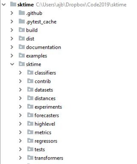
Figure 1: Overview of the current sktime file structure (sktime version 0.3).

Classifiers are grouped based on their core transformation technique.

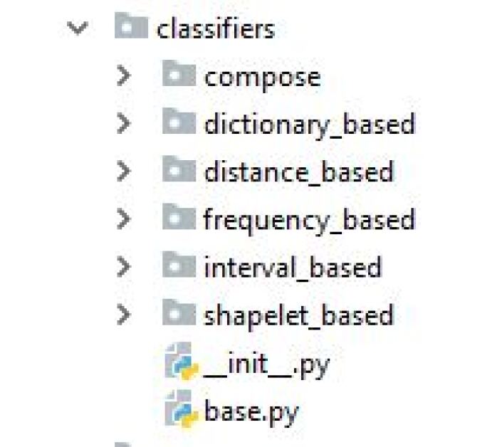
Figure 2: Overview of the current sktime classifier packages (sktime version 0.3).

The taxonomy of classifiers is taken from the comparative study presented in [3]. Currently, the following classifiers are available.

interval_based is a package for classifiers built on intervals of the series. Currently, it contains a single classifier the Time Series Forest [8], in file tsf.py. This is evaluated in Section 3. Spectral based classifiers are located in the package frequency_based. The random interval spectral ensemble (RISE) [17] is as yet the only concrete implementation of this type and it can be found in rise.py (see Section 4). dictionary_based contains classifiers that form histograms of discretised words. We have the Bag of SFA Symbols (BOSS) [23] classifier, implemented as BOSSEnsemble in boss.py, with experiments described in Section 5. Shapelets are discriminatory subseries, and classifiers that use them are in the shapelet_based package. We evaluate a version of the shapelet transform classifier [4] implemented in the file stc.py.

In time_series_neigbours.py there is KNeighborsTimeSeriesClassifier, an sklearn based nearest neighbour (NN) classifier that can be configured to use a range of distance measures, including: dynamic time warping (DTW); derivative dynamic time warping (DDTW) [10]; weighted DTW [13]; longest common subsequence; edit distance with penalty (ERP); and move-split-merge [26]. Until recently, DTW with 1-NN was by far the most commonly used benchmark algorithm for time series classification. These distance functions are available in the package distances. we evaluate the ElasticEnsemble [16], and ensemble of nearest neighbour classifiers using elastic distance measures, which is in elastic_ensemble.py. Furthermore, in proximity.py there is the
ProximityForest [19], a tree based classifier using a range of distance measures. DTW, EE and PF classifiers are evaluated in Section 7. The sktime experiments described in the following sections can be reproduced using the code in contrib/basic_benchmarking.py.

3 Interval Based: Time Series Forest (TSF) [8]

TSF is probably the simplest bespoke classifier and hence was the first algorithm we implemented. TSF is an ensemble of tree classifiers, each constructed on a different feature space. For any given ensemble member, a set of random intervals is selected, and three summary statistics (mean, standard deviation and slope) are calculated for each interval. The statistics for each interval are concatenated to form the new feature space.

In sktime, there are two ways of constructing a TSF estimator. The hard coded implementation TimeSeriesForest is in the file tsf.py. An example usage, including data loading and building, assuming full_path is where the problems reside, is as follows:

     from sktime.utils.load_data import load_from_tsfile_to_dataframe                                                      as load_ts  import sktime.classifiers.interval_based.tsf as ib  #method 1  tsf=ib.TimeSeriesForest(n_trees=100)  trainX, trainY = load_ts(full_path + ’_TRAIN.ts’)  testX, testY = load_ts(full_path  + ’_TEST.ts’)  tsf.fit(trainX, trainY)  predictions=tsf.predict(testX)  probabilities=tsf.predict_proba(testX)     Alternatively, you can configure the TimeSeriesForestClassifier in
classifiers.compose.ensemble.py as TSF as follows

     #method 2  steps = [   (’segment’, RandomIntervalSegmenter(n_intervals=’sqrt’)),   (’transform’, FeatureUnion([      (’mean’, RowwiseTransformer(FunctionTransformer(func=np.mean,                                  validate=False))),      (’std’, RowwiseTransformer(FunctionTransformer(func=np.std,                                  validate=False))),      (’slope’, RowwiseTransformer(                  FunctionTransformer(func=time_series_slope),                                      validate=False))   ])),   (’clf’, DecisionTreeClassifier())  ]  base_estimator = Pipeline(steps)  tsf = TimeSeriesForestClassifier(base_estimator=base_estimator,                                   n_estimators=100)     The validate=False is to stop the built in methods using the sktime data format incorrectly (and to suppress annoying warnings). It will be set by default to False in the next release. The configurable version allows for the easy formulation of TSF like variants and other transformation based ensembles. However, this comes at the cost of efficiency. To verify the implementations, we compare the tsml java version used in the bake off [3] to the two sktime versions.

We aim to show there is no difference in accuracy between the three implementations. We evaluate these three classifiers on 30 stratified resamples on 111 of the UCR archive [6].

Full results are available on the associated website. Figure LABEL:fig:tsf_cd shows the critical difference diagrams [7] for the three versions for accuracy, balanced accuracy, area under the receiver operator curve (AUC) and the negative log likelihood (NLL). Solid bars indicate ’cliques’, within which there is no significant difference between members. A fuller explanation is provided in [2]. Figure LABEL:fig:tsf_cd demonstrates there is no significant difference in between the classifiers in accuracy, balanced accuracy and NLL. The only observed difference is that sktime1 is significantly better than sktime2 with AUC. This may be explainable by the voting method employed by the two algorithms being different, although we have not confirmed it. We suspect this is just a chance result. The actual differences in AUC are very small.

(a) Accuracy	(b) Balanced Accuracy
(c) AUC	(d) NLL

Figure 3: Critical difference diagrams for three TSF implementations. Two from sktime (sktime1 using method 1 and sktime2 using method 2) and one from tsml. There is no significant difference between the three classifiers (as tested with a pairwise wilcoxon test with Holm correction, $\alpha=0.05$).

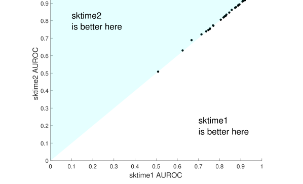
Figure 4: TSF sktime1 vs sktime2 scatterplot of AUC. sktime2 Wins/Draw/Losses: 41/5/65

Figures 5 and 6 shows the pairwise scatter plots for sktime2 vs tsml and sktime1.

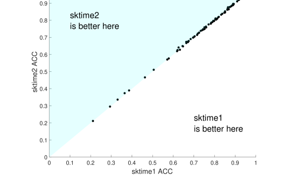
Figure 5: TSF sktime1 vs sktime2 scatterplot of test accuracies. sktime2 Wins/Draw/Losses: 59/5/47.

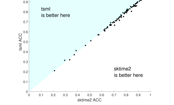
Figure 6: TSF tsml vs sktime2 scatterplot of test accuracies. sktime2 Wins/Draw/Losses: 60/3/48.

Timing comparison for the three classifiers is shown in Figure 7.

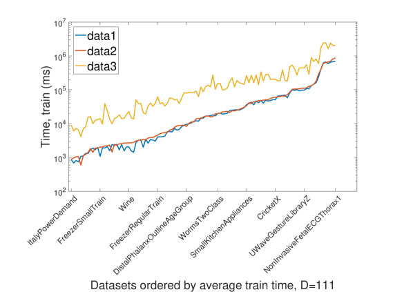
Figure 7: Train time for three TSF classifiers: sktime1 (data1); tsml (data2); and sktime2 (data3).

The configurable version is an order of magnitude slower than the fixed version, which is approximately equivalent to the java based tsml. We are not entirely sure as to the reason for this slowdown with the composite. We suspect it is due to excessive unpacking and packing of data into pandas, but it merits further investigation and detailed profiling, particularly as the accuracy is marginally, although not significantly, higher.

4 Frequency Based: RISE [17]

RISE is similar to TSF in that it is an ensemble of decision tree classifiers. The difference lies in the feature space used for each base classifier. RISE selects a single random interval for each base classifier, then transforms the time series in that interval into the power spectrum and autocorrelation features. As with TSF, there are two ways of building RISE.

     import sktime.classifiers.interval_based.tsf as ib  from sklearn.preprocessing import FunctionTransformer  from sklearn.tree import DecisionTreeClassifier  from statsmodels.tsa.stattools import acf  from sktime.transformers.compose import RowwiseTransformer  from sktime.transformers.segment import RandomIntervalSegmenter  from sktime.transformers.compose import ColumnTransformer  from sktime.transformers.compose import Tabulariser  from sktime.pipeline import Pipeline  from sktime.pipeline import FeatureUnion  from sktime.classifiers.compose import TimeSeriesForestClassifier    #method 1: fixed classifier  rise = fb.RandomIntervalSpectralForest(n_trees=100)       

     #method 2: configurable classifier  steps = [   (’segment’,RandomIntervalSegmenter(n_intervals=1, min_length=5)),   (’transform’,FeatureUnion([    (’acf’,RowwiseTransformer(FunctionTransformer(func=acf_coefs,                                                 validate=False))),    (’ps’,RowwiseTransformer(FunctionTransformer(func=powerspectrum,                                                 validate=False)))   ])),    (’tabularise’, Tabulariser()),    (’clf’, DecisionTreeClassifier())    ]  base_estimator = Pipeline(steps)  rise = TimeSeriesForestClassifier(base_estimator=base_estimator,                                      n_estimators=100)    def acf_coefs(x, maxlag=100):      x = np.asarray(x).ravel()      nlags = np.minimum(len(x) - 1, maxlag)      return acf(x, nlags=nlags).ravel()    def powerspectrum(x, **kwargs):      x = np.asarray(x).ravel()      fft = np.fft.fft(x)      ps = fft.real * fft.real + fft.imag * fft.imag      return ps[:ps.shape[0] // 2].ravel()     The composite version requires the definition of the acf and power spectrum functions. We will make this better encapsulated in the next release. To validate these implementations, we again benchmark against the tsml Java version, using RISE with 50 trees. Using the built in numpy functions for sktime2 creates a problem with some datasets: if a zero variance interval is passed to the numpy functions, an exception is thrown. In sktime1 and tsml we can manually adjust for this circumstance. The nature of the composite sktime2 makes this harder to manage. This means we are only able to compare on 68 datasets. Figures 8, 9 and 10 show there is no significant difference in accuracy between the three classifiers. However, there is greater variance in the difference in accuracy than observed for TSF.

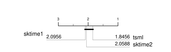
Figure 8: Average ranks for three RISE implementations. Two from sktime (sktime1 using method 1 and sktime2 using method 2) and one from tsml. There is no significant difference between the three classifiers (as tested with a pairwise wilcoxon test with Holm correction, $\alpha=0.05$).

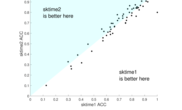
Figure 9: RISE sktime2 vs sktime1 scatterplot of test accuracies. sktime2 Wins/Draw/Losses: 34/5/29

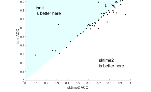
Figure 10: RISE tsml vs sktime2 scatterplot of test accuracies. sktime2 Wins/Draw/Losses: 25/5/38

The timing comparison for RISE, shown in Figure 11, highlights two curious characteristics. Firstly, sktime2 is an order of magnitude faster than both sktime1 and tsml. We believe this is due to to the efficient numpy implementations used, although it merits further investigation. Secondly, tsml has much higher variance than the sktime implementations, and seems to take an unexpectedly long time on some small problems. This also merits further investigation.

Figure 11: Train time for three RISE classifiers: sktime1 (data2); tsml (data3); and sktime2 (data1).

5 Dictionary Based: BOSS [23]

The BOSS implementation contains two components, BOSSIndividual and the BOSSEnsemble (what we refer to as BOSS). Individual BOSS classifiers create a histogram of words from each series using the SFA transform over sliding windows. A one nearest neighbour classifier using a bespoke BOSS distance is then used for classification. The BOSSEnsemble is an ensemble of BOSSIndividual classifiers. The ensemble members are selected through a grid search of individual BOSS parameters, with classifiers below 92% accuracy of the best classifier removed.

We also implement a faster and more configurable version of the classifier cBOSS [21], replacing the grid search with a filtered random selection. This alternative method can be employed with the BOSSEnsemble by setting the randomised_ensemble parameter to true. Two parameters are associated with this version: the number of individual BOSS classifiers to be built n_parameter_samples and the maximum number of classifiers in the ensemble max_ensemble_size. cBOSS is also contractable, allowing a unit of time in minutes using the time_limit parameter to replace the n_parameter_samples.

Examples of how to construct BOSS and cBOSS are demonstrated in the following code sample.

     import sktime.classifiers.dictionary_based.boss as db    # By default the original BOSS algorithm is setup  boss = db.BOSSEnsemble()    # Configuration for recommended cBOSS settings  c_boss = db.BOSSEnsemble(randomised_ensemble=True,                     n_parameter_samples=250, max_ensemble_size=50)    # cBOSS contracted for 1 hour, input time must be in minutes  c_boss_contract = db.BOSSEnsemble(randomised_ensemble=True,                               time_limit=60, max_ensemble_size=50)     

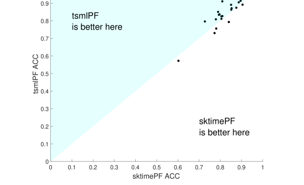
Figure 17: PF sktime vs tsml scatterplot of test accuracies.

Our primary goal is to test the correctness and efficiency of the standard implementations. To this end, we compare the implementations of BOSS in sktime and tsml. Figure 17 plots the accuracy of the two classifiers on 92 datasets. The accuracies are very similar (63 are identical and the differences are insignificant. We expected less variation in accuracy with the nearest neighbour classifier than the tree based classifiers, because there are fewer stochastic elements. This is indeed the case. However, the timing results displayed in Figure 18 show how much slower the sktime implementation is: approximately 10-40 times slower than tsml. This was also not unexpected. The implementation is mapped directly from Java and does not exploit any of the efficiency improvements that can be used in python. This is required future work.

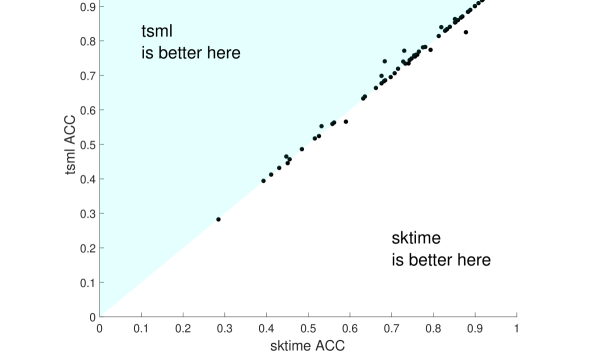
Figure 12: BOSS sktime vs tsml scatterplot of test accuracies. sktime Wins/Draw/Losses: 12/63/12.

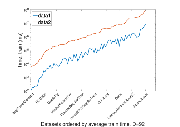
Figure 13: Train time for two BOSS classifiers: sktime (data2) and tsml (data1).

6 Shapelet Based: Shapelet Transform Classifier (STC) [11]

The shapelet transform classifier (ShapeletTransformClassifier in file stc.py) is a single pipeline of a shapelet transform (transformers/shapelets.py) and a classifier (by default, a random forest with 500 trees). The original shapelet transform performed a complete enumeration of the shapelet space, and used a heterogeneous ensemble for a classifier [11]. More recent research has shown that equivalent accuracy can be obtained through randomly searching for shapelets rather than a full enumeration [4]. The shapelet transform in sktime is contractable, in that you can specify an amount of time to search for shapelets before performing the transform. The default is 300 minutes. The latest STC in tsml uses a rotation forest classifier, since it has been shown to be best for this type of problem [2]. Rotation forest is not yet available in python (we are working on an alpha version), hence we use random forest for our comparison. We run STC in sktime and tsml with a 1000 minute time limit and use the sklearn amd Weka random forest implementations as the final classifier. Given both classifiers are contracted, we only compare the accuracies. Figure 14 shows that, overall, there is no significant difference between the two implementations. However, there is still some considerable variation. This may be down to evaluation over a single resample, or related to core differences in the underlying implementation. Further investigation is required.

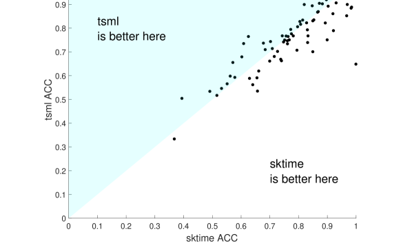
Figure 14: STC sktime vs tsml scatterplot of test accuracies. sktime Wins/Draw/Losses: 48/11/52

7 Distance Based: Elastic Ensemble (EE) and Proximity Forest (PF)

7.1 Elastic Ensemble [16]

The Elastic Ensemble (EE) [16] ensembles 11 different time series distance measures each coupled with a 1-nearest-neighbour (NN) classifier, together known as the constituents of EE. The variation in distance measure of each constituent injects diversity into the ensemble and provides superior classification performance over any individual constituent alone. EE uses the following distance measures: Euclidean distance, Dynamic Time Warping (DTW), Derivative DTW (DDTW) [15], DTW with cross-validated warping window (DTWCV) [22], DDTW with cross-validated warping window (DDTWCV), Lowest Common Sub-Sequence (LCSS) [12], Edit Distance with Real Penalty (ERP) [5], Move-Split-Merge (MSM) [26], and Time Warp Edit Distance (TWED) [20]. The latter eight of these distance measures benefit from hyper-parameter tuning. By default, EE employs a tuning process for each constituent over 100 parameter options using leave-one-out-cross-validation (LOOCV).

Comparing long time-series using distance measures can be time consuming, therefore both a cython and python version are provided in sktime. These are in distances.elastic.py and distances.elastic_cython.pyx. Further, sktime provides an extension to scikit-learn’s KNeighborsClassifier to enable usage with pandas dataframes and custom distance measures. The tuning of each constituent of EE can be time consuming also, therefore we provide capability to reduce the number of neighbours used in examination of parameter options and reduce the number of parameters per constituent overall. Both of these have been shown to significantly speed-up EE with no significant loss in classification performance.

         from sktime.classifiers.distance_based.elastic_ensemble          import ElasticEnsemble      from sktime.classifiers.distance_based.time_series_neighbors          import KNeighborsTimeSeriesClassifier      from sklearn.model_selection          import GridSearchCV,                 LeaveOneOut        # 1NN classifier with full DTW as the distance measure      dtw_nn = KNeighborsTimeSeriesClassifier(metric=’dtw’,          n_neighbors=1)        # 1NN classifier tuned for best accuracy over 100 DTW      # warping window options      dtwcv_nn = GridSearchCV(          estimator=KNeighborsTimeSeriesClassifier(metric=’dtw’,              n_neighbors=1),          param_grid={’metric_params’:              [{’w’: x / 100} for x in range(0, 100)]}          cv=LeaveOneOut(),          scoring=’accuracy’      )        # Default EE with full tuning effort      ee = ElasticEnsemble()        # Configuration for reducing tuning efforts of the EE      ee = ElasticEnsemble(proportion_of_param_options = 0.5,           proportion_of_train_in_param_finding = 0.1)     Even with cython, the full Elastic Ensemble is very slow in both absolute and relative terms. In practice, we never run it as a single classifier. Rather, we build each constituent in parallel and ensemble after each is complete.

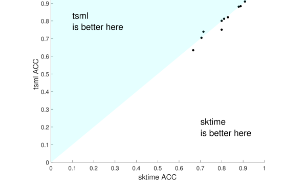
Figure 15: EE sktime vs tsml scatterplot of test accuracies.

Figure 16: Train time for two EE classifiers: sktime (data2) and tsml (data1).

7.2 Proximity Forest

Proximity Forest (PF) [19] is a competitor to EE and implements a forest of decision trees, known as Proximity Trees (PT), in a Random Forest like structure. A Proximity Tree (PT) partitions data by comparing the relative similarity of instances against a set of exemplar instances. At any given node in the PT, a one exemplar instance is randomly picked per class from the data passed down from the parent node. The data is partitioned based upon the similarity of data instances against exemplar instances, grouping similar instances. Each group of instances, along with the corresponding exemplar, are passed down as input data to a child node and the process repeats until leaf nodes are pure. This process is known as splitting.

The similarity of instances against exemplar instances is determined using distance measures. PF uses the same distance measures and corresponding parameter ranges as EE. Each split in a PT randomly chooses the distance measure and corresponding parameter set if required. This randomness can lead to poor splits, therefore a hyperparameter $r$ controls the evaluation of multiple splits at each node, choosing the best split based upon gini score. Each split can be seen as a PT of height 1, otherwise known as a Proximity Stump (PS).

The PF generates a set number of PTs and combines their predictions using a majority vote. The extreme randomisation across the PF produces classifier which can be built in a fraction of the time of EE and produce competitive prediction performance.

         from sktime.classifiers.distance_based.proximity_forest          import ProximityForest,                 ProximityStump,                 ProximityTree        # Proximity Stump (PT with 1 level of depth)      ps = ProximityStump()        # Proximity Tree with 5 split evaluations per tree node      pt = ProximityTree(n_stump_evaluations = 5)        # Proximity Forest with 100 trees and      #   5 split evaluations per tree node      pf = ProximityForest(n_trees = 100, n_stump_evaluations = 5)     

Figure 18: Train time for two PF classifiers: sktime (data2) and tsml (data1).

8 Conclusions and Future Directions

Developing time series classification algorithms is an active research field. Our goal in providing sktime is to make researching this field easier and more transparent. If researchers use a common framework, reproducability and comparison to the current state of the art becomes easy. In this way we hope to drive the field forward to help automatically answer the key questions for classifying time series: which is the best algorithm for the task at hand.

The classification component of sktime has broad functionality, but there is much that could be added and improved. Our work plan for the medium term is as follows.

8.1 Improved Classifier Functionality

It has taken a surprising amount of effort to get this far, but there is still much to do. This exercise has highlighted several issues with sktime that need resolving before the next release to master.

1. interval based: why is the composite version so much slower than the others?

2. frequency based: can we speed up RISE through matrix operations without exception being continually thrown?

3. dictionary based: can we speed up BOSS through a more pythonesque implementation?

4. shapelet based: can we improve accuracy by using rotation forest and improving the search efficiency through cython?

5. Can we improve EE performance through restricting the parameter search?

We also intend to improve the functionality by making all classifiers contractable and allow for efficient estimation of the test error from the train data. In addition to improving the existing set of classifiers in these ways, we intend porting in recently proposed alternative TSC algorithms such as FastEE, TS-CHIEF [25], WEASEL [24], Shapelet Forest [14] and HIVE-COTE [17]. We have implemented the range of distance functions and kernels described in [1] and the Matrix Profile distance MPDist [9]. We will evaluate these classifiers to examine how they perform in relation to those already implemented within the toolkit.

8.2 Handle Unequal Length Series

One of the primary motivators for our data model of pandas of series objects was to facilitate the easy incorporation of unequal length time series as classification problems. The current suite of available algorithms needs to be adjusted to allow for this use case. For some algorithms this will be fairly simple: BOSS, for example, can simply normalise the histograms and shapelets are independent of series length. However, these design choices may have an impact on accuracy and experimentation using the enhancements will be required.

8.3 Multivariate Time Series Classifiers

sktime already provides two composition interfaces for solving multivariate time series classification problems, including

• the ColumnConcatenator, a transformer that can be used to concatenate two or more time series columns into a single long time series column, so that one can then apply a classifier to the concatenated, univariate data, and

• the ColumnEnsembleClassifier, a meta-estimator that allows for column-wise ensembling in which a separate classifier is fitted for each time series column and their predictions are aggregated.

We have started to implement bespoke methods for specific estimators to handle multivariate time series input data and we aim to add more bespoke methods in future work, e.g. finding shapelets in multidimensional space or extending time series forest to extract features from multidimensional segments (or hyper-planes). There are also a multitude of bespoke methods for classifying time series. We shall draw up a candidate

8.4 Time series regression

The composite structure of many time series classifiers allows us to refactor them into their regressor counterparts. We have started implementing regression algorithms, including a TSF regressor and are currently working on adding more regressors.

References

- [1] A. Abanda, U. Mori, and J. Lozano. A review on distance based time series classification. Data Mining and Knowledge Discovery, 33(2):378–412, 2019.
- [2] A. Bagnall, A. Bostrom, G. Cawley, M. Flynn, J. Large, and J. Lines. Is rotation forest the best classifier for problems with continuous features? ArXiv e-prints, arXiv:1809.06705, 2018.
- [3] A. Bagnall, J. Lines, A. Bostrom, J. Large, and E. Keogh. The great time series classification bake off: a review and experimental evaluation of recent algorithmic advances. Data Mining and Knowledge Discovery, 31(3):606–660, 2017.
- [4] A. Bostrom and A. Bagnall. Binary shapelet transform for multiclass time series classification. Transactions on Large-Scale Data and Knowledge Centered Systems, 32:24–46, 2017.
- [5] L. Chen and R. Ng. On the marriage of Lp-norms and edit distance. In Proc. 30th International Conference on Very Large Databases (VLDB), 2004.
- [6] H. Dau, A. Bagnall, K. Kamgar, M. Yeh, Y. Zhu, S. Gharghabi, and C. Ratanamahatana. The UCR time series archive. ArXiv e-prints, arXiv:1810.07758, 2018.
- [7] J. Demšar. Statistical comparisons of classifiers over multiple data sets. Journal of Machine Learning Research, 7:1–30, 2006.
- [8] H. Deng, G. Runger, E. Tuv, and M. Vladimir. A time series forest for classification and feature extraction. Information Sciences, 239:142–153, 2013.
- [9] S. Gharghabi, S. Imani, A. Bagnall, A. Darvishzadeh, and E. Keogh. Matrix Profile XII: MPDist: A novel time series distance measure to allow data mining in more challenging scenarios. In Proc. 18th IEEE International Conference on Data Mining, 2018.
- [10] T. Górecki and M. Łuczak. Using derivatives in time series classification. Data Mining and Knowledge Discovery, 26(2):310–331, 2013.
- [11] J. Hills, J. Lines, E. Baranauskas, J. Mapp, and A. Bagnall. Classification of time series by shapelet transformation. Data Mining and Knowledge Discovery, 28(4):851–881, 2014.
- [12] D. Hirschberg. Algorithms for the longest common subsequence problem. Journal of the ACM, 24(4):664–675, 1977.
- [13] Y. Jeong, M. Jeong, and O. Omitaomu. Weighted dynamic time warping for time series classification. Pattern Recognition, 44:2231–2240, 2011.
- [14] I. Karlsson, Papapetrou P, and H. Boström. Generalized random shapelet forests. Data Mining and Knowledge Discovery, 30(5):1053–1085, 2016.
- [15] E. Keogh and M. Pazzani. Derivative dynamic time warping. In Proc. 1st SIAM International Conference on Data Mining (SDM), 2001.
- [16] J. Lines and A. Bagnall. Time series classification with ensembles of elastic distance measures. Data Mining and Knowledge Discovery, 29:565–592, 2015.
- [17] J. Lines, S. Taylor, and A. Bagnall. Time series classification with HIVE-COTE: The hierarchical vote collective of transformation-based ensembles. ACM Trans. Knowledge Discovery from Data, 12(5), 2018.
- [18] Markus Löning, Anthony Bagnall, Sajaysurya Ganesh, Viktor Kazakov, Jason Lines, and Franz J. Király. A unified interface for machine learning with time series. ArXiv e-prints, arXiv:1909.07872, 2019.
- [19] B. Lucas, A. Shifaz, C. Pelletier, L. O’Neill, N. Zaidi, B. Goethals, F. Petitjean, and G. Webb. Proximity forest: an effective and scalable distance-based classifier for time series. Data Mining and Knowledge Discovery, 33(3):607–635, 2019.
- [20] P. Marteau. Time warp edit distance with stiffness adjustment for time series matching. IEEE Transactions on Pattern Analysis and Machine Intelligence, 31(2):306–318, 2009.
- [21] M. Middlehurst, W. Vickers, and A. Bagnall. Scalable dictionary classifiers for time series classification. arXiv preprint arXiv:1907.11815, 2019.
- [22] C. Ratanamahatana and E. Keogh. Three myths about dynamic time warping data mining. In Proc. 5th SIAM International Conference on Data Mining, 2005.
- [23] P. Schäfer. The BOSS is concerned with time series classification in the presence of noise. Data Mining and Knowledge Discovery, 29(6):1505–1530, 2015.
- [24] P. Schäfer and U. Leser. Fast and accurate time series classification with weasel. In Proceedings of the 2017 ACM on Conference on Information and Knowledge Management, pages 637–646. ACM, 2017.
- [25] A. Shifaz, C. Pelletier, F. Petitjean, and G. Webb. TS-CHIEF: A scalable and accurate forest algorithm for time series classification. ArXiv e-prints, arXiv:1906.10329, 2019.
- [26] A. Stefan, V. Athitsos, and G. Das. The Move-Split-Merge metric for time series. IEEE Transactions on Knowledge and Data Engineering, 25(6):1425–1438, 2013.