2-loop RG evolution of $\mathcal{CP}$-violating 2HDM

Abstract

We use the recently developed code 2HDME to perform a 2-loop renormalization group analyzis of the $\mathcal{CP}$ violating Two-Higgs-doublet model (2HDM). Using parameter scans of several scenarios of $\mathbb{Z}_{2}$ symmetry breaking, we investigate the properties of 2HDMs under renormalization group evolution. Collider data constraints are implemented with HiggsBounds and HiggsSignals and we include all the important Barr-Zee diagram contributions to the electron’s electric dipole moment to put limits on the $\mathcal{CP}$ violation that is allowed both in the scalar and the Yukawa sector. As a result, we see that the $\mathcal{CP}$ violation spreads easily across the sectors during renormalization group evolution when one breaks the $\mathbb{Z}_{2}$ symmetry in either sector, putting additional constraints on the $\mathcal{CP}$ violating parameters.

1 Introduction

The Two-Higgs-Doublet Model (2HDM) is one of the most studied minimalistic extensions of the Standard Model (SM) of particle physics and serves as an effective theory for many Beyond the SM (BSM) models. It offers a rich scalar sector with its three neutral plus a charged pair of Higgs bosons. One of the neutral ones should make up the 125 GeV scalar particle that has been discovered at the Large Hadron Collider (LHC) by the ATLAS Aad:2012tfa and CMS Chatrchyan:2012xdj collaborations; that, so far, resembles the SM Higgs boson Khachatryan:2016vau . According to the LHC data, it is ruled out that the discovered particle is a pure $\mathcal{CP}$ odd scalar Khachatryan:2014kca ; however, there is still the possibility that it is a mixture of $\mathcal{CP}$ even and $\mathcal{CP}$ odd states.

While the 2HDM is well studied in the literature, it is most often the $\mathcal{CP}$ conserving one even though the 2HDM exhibits the possibility of $\mathcal{CP}$ violation. It is well known that, to fulfill the Sakharov’s criteria for baryogenesis Sakharov:1967dj , new sources of $\mathcal{CP}$ violation are needed to sufficiently explain the excess of matter over anti-matter in the universe. The possibility for $\mathcal{CP}$ violation in the 2HDM is therefore an intriguing feature, which was the original motivation for studying the 2HDM in the first place Lee:1973iz .

There are several experiments that limit the amount of $\mathcal{CP}$ violation one can have in the 2HDM. One of the most troublesome observables is that one easily generates a large Electric Dipole Moments (EDMs) for particles; which are severely constrained by experiments. The electron’s EDM (eEDM) has recently received an upper limit from the ACMEII collaboration Andreev:2018ayy ,

$$|d_{e}|<1.1\times 10^{-29}~{}\text{e cm}.$$ (1)

Another well known problem of the general 2HDM, not exclusive to the $\mathcal{CP}$ violating case, is the presence of Flavor-Changing-Neutral currents (FCNCs) and one popular solution is to impose a $\mathbb{Z}_{2}$ symmetry on the model Glashow:1976nt ; Paschos:1976ay ; although, often one allows for a soft $\mathbb{Z}_{2}$ symmetry breaking term.

In recent years, the softly broken $\mathbb{Z}_{2}$ symmetric 2HDM has been confronted with data from the LHC as well as the limits coming from EDMs Shu:2013uua ; Jung:2013hka ; Inoue:2014nva ; Cheung:2014oaa ; Ipek:2013iba ; Bian:2014zka ; Chen:2015gaa ; Fontes:2017zfn ; Egana-Ugrinovic:2018fpy . In this work, we investigate the complex, $\mathcal{CP}$ violating, 2HDM by probing its behavior under Renormalization Group (RG) evolution, while also revisiting the constraints from collider data and the eEDM. We focus on RG effects such as how different choices of $\mathbb{Z}_{2}$  symmetry can affect the energy range of validity and look for any symmetry breaking, or $\mathcal{CP}$ violation, that spreads across the Yukawa and scalar sectors.

There are many studies that analyze the 2HDM using 1-loop RG Equations (RGEs), e.g. refs. Dev:2014yca ; Penuelas:2017ikk ; Botella:2018gzy ; Gori:2017qwg ; Basler:2017nzu ; Ferreira:2015rha ; Bijnens:2011gd , but also some that use the 2-loop ones Chowdhury:2015yja ; Krauss:2018thf ; Oredsson:2018yho . We use the code 2HDME Oredsson:2018vio to perform the RG evolution at 2-loop order. It is essential to go to 2-loop order if one is interested in studying how all sectors affect each other during RG evolution; since the quartic couplings enter the Yukawa couplings’ RG Equations (RGEs) first at this order.

To investigate the parameter space of the 2HDM, we set up numerical parameter scans of different physical scenarios; each with their own level of $\mathbb{Z}_{2}$ symmetry in each sector. In addition to looking for Landau poles in the RG evolution, we perform tree-level checks of unitarity and stability. We also compute the oblique parameters $S$, $T$ and $U$; as well as the branching ratios for all Higgs decays with a modified version of 2HDMC Eriksson:2009ws . To check whether a parameter point is excluded by collider data, we use the codes HiggsBounds Bechtle:2008jh ; Bechtle:2011sb ; Bechtle:2013wla and HiggsSignals Bechtle:2013xfa . Finally, we use the eEDM as an additional constraint on the amount of $\mathcal{CP}$ violation. We calculate this observable by summing up all the relevant Barr-Zee diagrams Barr:1990vd that contribute. This calculation is also implemented in a recent update of 2HDME.

This paper is structured as follows: we begin in section 2 by giving a brief review of the 2HDM and present the notation that we use. We describe the different scenarios of parameter scans in section 3. The constraints that we implement are listed in section 4. To illustrate the characteristic change in behavior of the 2HDM when allowing for $\mathcal{CP}$ violation, we vary the amount of $\mathcal{CP}$ violation in an example point in section 5 and look at various observables. The main results of the parameter scans are presented in section 6 and we subsequently summarize our conclusions in section 7. Some plots of the generic basis of 2HDM in the first scenario are collected in appendix A. In appendix B, we list all the formulas for every Barr-Zee diagram that we use to calculate the eEDM.

2 The 2HDM

Since 2HDM is one of the most studied BSM theories, we will only briefly describe it here and for a full review we refer to ref. Branco:2011iw . Throughout this work, we use the notation employed in the basis independent treatment of the 2HDM in refs. Davidson:2005cw ; Haber:2006ue ; Haber:2010bw .

The most general gauge invariant renormalizable scalar potential for two hypercharge $+1/2$ Higgs doublets, $\Phi_{1,2}$, can be written

$$-\mathcal{L}_{V}= m_{11}^{2}\Phi_{1}^{\dagger}\Phi_{1}+m_{22}^{2}\Phi_{2}^{\dagger}\Phi_{2}-(m_{12}^{2}\Phi_{1}^{\dagger}\Phi_{2}+\text{h.c.})+\frac{1}{2}\lambda_{1}\left(\Phi_{1}^{\dagger}\Phi_{1}\right)^{2}+\frac{1}{2}\lambda_{2}\left(\Phi_{2}^{\dagger}\Phi_{2}\right)^{2}$$

$$+\lambda_{3}\left(\Phi_{1}^{\dagger}\Phi_{1}\right)\left(\Phi_{2}^{\dagger}\Phi_{2}\right)+\lambda_{4}\left(\Phi_{1}^{\dagger}\Phi_{2}\right)\left(\Phi_{2}^{\dagger}\Phi_{1}\right)$$

$$+\left[\frac{1}{2}\lambda_{5}\left(\Phi_{1}^{\dagger}\Phi_{2}\right)^{2}+\lambda_{6}\left(\Phi_{1}^{\dagger}\Phi_{1}\right)\left(\Phi_{1}^{\dagger}\Phi_{2}\right)+\lambda_{7}\left(\Phi_{2}^{\dagger}\Phi_{2}\right)\left(\Phi_{1}^{\dagger}\Phi_{2}\right)+\text{h.c.}\right],$$ (2)

where $m_{12}^{2}$ and $\lambda_{5,6,7}$ are potentially complex while all the other parameters are real; resulting in a total of 14 degrees of freedom.

After electroweak symmetry breaking, $SU(2)\times U(1)_{Y}\rightarrow U(1)_{\text{em}}$, both the scalar fields acquire a Vacuum Expectation Value (VEV). Using global $SU(2)_{L}$ and $U(1)$ rotations, the fields’ VEV take the forms

$$\left\langle\Phi_{1}\right\rangle=\frac{1}{\sqrt{2}}\left(\begin{array}[]{c}0\\ v_{1}\end{array}\right) \left\langle\Phi_{2}\right\rangle=\frac{1}{\sqrt{2}}\left(\begin{array}[]{c}0\\ v_{2}e^{i\xi}\end{array}\right),$$ and (7)

where $v=\sqrt{v_{1}^{2}+v_{2}^{2}}\approx 246$ GeV and we define $\tan\beta\equiv t_{\beta}\equiv v_{2}/v_{1}$. By convention, we take $0\leq\beta\leq\pi/2$ and $0\leq\xi\leq 2\pi$. Note that, if the two Higgs fields are identical by having equal quantum numbers, one is free to perform a Higgs flavor basis transformation and $\tan\beta$ is an unphysical parameter Haber:2006ue .

Minimizing the potential results in the tadpole equations

$$m_{11}^{2}=~{} m_{12}^{2}e^{i\xi}t_{\beta}-\frac{1}{2}v^{2}\left[\lambda_{1}c_{\beta}^{2}+(\lambda_{3}+\lambda_{4}+\lambda_{5}e^{2i\xi})s_{\beta}^{2}\right.$$

$$\hskip 85.35826pt\left.+(2\lambda_{6}e^{i\xi}+\lambda_{6}^{*}e^{-i\xi})s_{\beta}c_{\beta}+\lambda_{7}s_{\beta}^{2}t_{\beta}e^{i\xi}\right],$$ (8)

$$m_{22}^{2}=~{} m_{12}^{2}e^{i\xi}t_{\beta}^{-1}-\frac{1}{2}v^{2}\left[\lambda_{2}s_{\beta}^{2}+(\lambda_{3}+\lambda_{4}+\lambda_{5}^{*}e^{-2i\xi})c_{\beta}^{2}\right.$$

$$\hskip 85.35826pt\left.+(\lambda_{7}e^{i\xi}+2\lambda_{7}^{*}e^{-i\xi})s_{\beta}c_{\beta}+\lambda_{6}^{*}c_{\beta}^{2}t_{\beta}^{-1}e^{-i\xi}\right],$$ (9)

$$\text{Im}(m_{12}^{2}e^{i\xi})=~{} \frac{1}{2}v^{2}\left[\text{Im}(\lambda_{5}e^{2i\xi})s_{\beta}c_{\beta}+\text{Im}(\lambda_{6}e^{2i\xi})c_{\beta}^{2}+\text{Im}(\lambda_{7}e^{i\xi})s_{\beta}^{2}\right].$$ (10)

These are used to fix $m_{11}^{2}$, $m_{22}^{2}$ and $\xi$.

2.1 The Higgs basis

In eq. (2) the general scalar potential for the 2HDM is written in the generic basis. Another basis is the Higgs basis Branco:1999fs ; Davidson:2005cw , where only one Higgs field gets a VEV. The Higgs basis fields in terms of the previously defined generic basis fields are

$$H_{1}\equiv\hat{v}_{\bar{a}}^{*}\Phi_{a}, H_{2}\equiv\hat{w}_{\bar{a}}^{*}\Phi_{a},$$ (11)

where $\hat{w}_{b}\equiv\hat{v}_{\bar{a}}^{*}\epsilon_{ab}$ ( $\epsilon_{12}=-\epsilon_{21}=1$) and

$$\hat{v}_{a}\equiv\left(\begin{array}[]{c}c_{\beta}\\ s_{\beta}e^{i\xi}\end{array}\right).$$ (14)

These fields acquire the VEVs

$$\left\langle H_{1}^{0}\right\rangle=v/\sqrt{2}, \left\langle H_{2}^{0}\right\rangle=0.$$ (15)

The scalar potential in the Higgs basis takes a similar form as in the generic basis,

$$-\mathcal{L}_{V}=~{} Y_{1}H_{1}^{\dagger}H_{1}+Y_{2}H_{2}^{\dagger}H_{2}+\left(Y_{3}H_{1}^{\dagger}H_{2}+\text{h.c.}\right)+\frac{1}{2}Z_{1}(H_{1}^{\dagger}H_{1})^{2}+\frac{1}{2}Z_{2}(H_{2}^{\dagger}H_{2})^{2}$$

$$+\frac{1}{2}Z_{3}(H_{1}^{\dagger}H_{1})(H_{2}^{\dagger}H_{2})+\frac{1}{2}Z_{4}(H_{1}^{\dagger}H_{2})(H_{2}^{\dagger}H_{1})$$

$$+\left\{\frac{1}{2}Z_{5}(H_{1}^{\dagger}H_{2})^{2}+\left[Z_{6}(H_{1}^{\dagger}H_{1})+Z_{7}(H_{2}^{\dagger}H_{2})\right]H_{1}^{\dagger}H_{2}+\text{h.c.}\right\},$$ (16)

where $Y_{3}$ and $Z_{5,6,7}$ are potentially complex. The tree-level tadpole equations are given by

$$Y_{1}=-\frac{1}{2}Z_{1}v^{2}, Y_{3}=-\frac{1}{2}Z_{6}v^{2}.$$ (17)

The Higgs basis is unique up to a rephasing of $H_{2}$. During a Higgs flavor transformation of the generic basis, $\Phi_{a}\rightarrow U_{a\bar{b}}\Phi_{b}$, the Higgs fields transform as Haber:2006ue

$$H_{1}\rightarrow H_{1}, H_{2}\rightarrow(\det U)H_{2}.$$ (18)

Thus from inspection of the Higgs potential in eq. (2.1), it follows that $Y_{1,2},Z_{1-4}$ are invariant, while

$$\{Y_{3},Z_{6,7}\}\rightarrow(\det U)^{-1}\{Y_{3},Z_{6,7}\}, Z_{5}\rightarrow(\det U)^{-2}Z_{5}$$ (19)

are pseudo-invariants under the Higgs flavor transformation.

The Higgs doublets are expanded around the VEV and parameterized as

$$H_{1}=\left(\begin{array}[]{c}G^{+}\\ \frac{1}{\sqrt{2}}(v+\phi_{1}^{0}+iG^{0})\end{array}\right) H_{2}=\left(\begin{array}[]{c}G^{+}\\ \frac{1}{\sqrt{2}}(\phi_{2}^{0}+ia^{0})\end{array}\right),$$ and (24)

where $G^{0,+}$ are Goldstone bosons that will be eaten by $Z$ and $W^{\pm}$. The physical scalar degrees of freedom, after electroweak symmetry breaking, correspond to three neutral ones that we will order according to their mass and denote as $h_{1,2,3}$; and one $U(1)_{em}$ charged pair of Higgs bosons that we will denote as $H^{\pm}$. In the $\mathcal{CP}$-conserving case, the neutral mass eigenstates have definite $\mathcal{CP}$ properties; while all the neutral Higgs bosons mix and have indefinite $\mathcal{CP}$ properties in the $\mathcal{CP}$ violating case. The neutral mass matrix in the $\phi_{1}^{0}-\phi_{2}^{0}-a^{0}$ basis is

$$\mathcal{M}=v^{2}\left(\begin{array}[]{ccc}Z_{1}&\mathrm{Re}\left(Z_{6}\right)&-\mathrm{Im}\left(Z_{6}\right)\\ \mathrm{Re}\left(Z_{6}\right)&\frac{1}{2}\left[Z_{3}+Z_{4}+\mathrm{Re}\left(Z_{5}\right)\right]+Y_{2}/v^{2}&-\frac{1}{2}\mathrm{Im}\left(Z_{5}\right)\\ -\mathrm{Im}\left(Z_{6}\right)&-\frac{1}{2}\mathrm{Im}\left(Z_{5}\right)&\frac{1}{2}\left[Z_{3}+Z_{4}-\mathrm{Re}\left(Z_{5}\right)\right]+Y_{2}/v^{2}\end{array}\right),$$ (28)

which can be diagonalized with the rotation matrix

$$R=\left(\begin{array}[]{ccc}c_{12}c_{13}&-s_{12}c_{23}-c_{12}s_{13}s_{23}&-c_{12}c_{23}s_{13}+s_{12}s_{23}\\ s_{12}c_{13}&c_{12}c_{23}-s_{12}s_{13}s_{23}&-s_{12}c_{23}s_{13}-c_{12}s_{23}\\ s_{13}&c_{13}s_{23}&c_{13}c_{23}\end{array}\right),$$ (32)

where $s_{ij}(c_{ij})$ denotes $\sin\theta_{ij}(\cos\theta_{ij})$. From these angles, one can construct the Higgs flavor independent quantities $q_{kl}$ Davidson:2005cw :

$k$	$q_{k1}$	$q_{k2}$
1	$c_{12}c_{13}$	$-s_{12}-ic_{12}s_{13}$
2	$s_{12}c_{13}$	$c_{12}-is_{12}s_{13}$
3	$s_{13}$	$ic_{13}$
4	$i$	$0$

,

which we will use to parametrize various couplings. The angle $\theta_{23}$ is however not invariant under a $U(2)$ Higgs flavor transformation, but instead obeys

$$e^{i\theta_{23}}\rightarrow(\det U)^{-1}e^{i\theta_{23}}.$$ (33)

2.2 The Yukawa sector

In this work, we do not include any mechanism to provide masses for the neutrinos. The Yukawa sector that couples the Higgs fields to the fermion fields is in the generic basis

$$-\mathcal{L}_{Y}= \bar{Q}_{L}^{0}\cdot\tilde{\Phi}_{\bar{a}}\eta_{a}^{U,0}U_{R}^{0}+\bar{Q}_{L}^{0}\cdot\Phi_{a}\eta_{\bar{a}}^{D,0\dagger}D_{R}^{0}+\bar{L}_{L}^{0}\cdot\Phi_{a}\eta_{\bar{a}}^{L,0\dagger}E_{R}^{0}+\text{h.c.}~{},$$ (34)

where the left-handed fermion fields in the weak eigenbasis are

$$Q_{L}^{0}\equiv\left(\begin{array}[]{c}U_{L}^{0}\\ D_{L}^{0}\end{array}\right), L_{L}^{0}\equiv\left(\begin{array}[]{c}\nu_{L}^{0}\\ E_{L}^{0}\end{array}\right)$$ (39)

and $\tilde{\Phi}\equiv i\sigma_{2}\Phi^{*}$.

In the Higgs basis, the Yukawa sector takes the form

$$-\mathcal{L}_{Y}=~{} \bar{Q}_{L}\tilde{H}_{1}\kappa^{U}U_{R}+\bar{Q}_{L}H_{1}\kappa^{D\dagger}D_{R}+\bar{L}_{L}H_{1}\kappa^{L\dagger}E_{R}$$

$$+\bar{Q}_{L}\tilde{H}_{2}\rho^{U}U_{R}+\bar{Q}_{L}H_{2}\rho^{D\dagger}D_{R}+\bar{L}_{L}H_{2}\rho^{L\dagger}E_{R}+\text{h.c.},$$ (40)

where we have performed a biunitary transformation to go to the fermion mass eigenbasis such that the $\kappa^{F}=V_{L}^{F}\kappa^{F,0}V_{R}^{F\dagger}$ matrices are diagonal. In the end, the $\kappa^{F}$ matrices are related to $\eta^{F}$ by

$$\kappa^{U}=~{} \hat{v}_{\bar{a}}^{*}\eta_{a}^{U}=\frac{\sqrt{2}}{v}\text{diag}(m_{u},m_{c},m_{t}),$$

$$\kappa^{D}=~{} \hat{v}_{\bar{a}}^{*}\eta_{a}^{D}=\frac{\sqrt{2}}{v}\text{diag}(m_{d},m_{s},m_{b}),$$

$$\kappa^{L}=~{} \hat{v}_{\bar{a}}^{*}\eta_{a}^{L}=\frac{\sqrt{2}}{v}\text{diag}(m_{e},m_{\mu},m_{\tau}),$$ (41)

and $\rho^{F}=\hat{w}_{\bar{a}}^{*}\eta_{a}^{F}$, where

$$\eta_{a}^{F}\equiv V_{L}^{F}\eta_{a}^{F,0}V_{R}^{F\dagger}.$$ (42)

The unitarity transformation matrices are defined by

$$F_{L}\equiv V_{L}^{F}F_{L}^{0}, F_{R}\equiv V_{R}^{F}F_{R}^{0},$$ (43)

where $F\in\{U,D,E\}$ denotes each fermion species. The CKM matrix is composed out of the left-handed transformation matrices, $V_{CKM}\equiv V_{L}^{U}V_{L}^{D\dagger}$.

The $\kappa^{F}$ matrices are, of course, invariant under Higgs flavor transformations, while $\rho^{F}$ transforms as

$$\rho^{F}\rightarrow(\det U)\rho^{F}.$$ (44)

In general, each $\rho^{F}$ is left as an arbitrary 3-by-3 complex matrix.

Couplings to mass eigenstates

We parameterize the couplings of neutral Higgs bosons, $k=1,2,3$, to fermions as

$$-\mathcal{L}=\bar{F}\left(c_{k}^{F}+\tilde{c}_{k}^{F}i\gamma_{5}\right)Fh_{k},$$ (45)

where $F$ corresponds to $U$, $D$ and $L$, which are the Dirac fermions as vectors in generation space. These couplings can be expressed in a basis-independent way as

$$c_{k}^{U}=~{} \frac{1}{\sqrt{2}}\left[\kappa^{U}q_{k1}+\frac{1}{2}(q_{k2}^{*}e^{i\theta_{23}}\rho^{U}+q_{k2}e^{-i\theta_{23}}\rho^{U\dagger})\right],$$ (46)

$$\tilde{c}_{k}^{U}=~{} \frac{i}{2\sqrt{2}}\left(q_{k2}e^{-i\theta_{23}}\rho^{U\dagger}-q_{k2}^{*}e^{i\theta_{23}}\rho^{U}\right),$$ (47)

$$c_{k}^{D}=~{} \frac{1}{\sqrt{2}}\left[\kappa^{D}q_{k1}+\frac{1}{2}(q_{k2}^{*}e^{i\theta_{23}}\rho^{D}+q_{k2}e^{-i\theta_{23}}\rho^{D\dagger})\right],$$ (48)

$$\tilde{c}_{k}^{D}=~{} \frac{i}{2\sqrt{2}}\left(q_{k2}^{*}e^{i\theta_{23}}\rho^{D}-q_{k2}e^{-i\theta_{23}}\rho^{D\dagger}\right),$$ (49)

$$c_{k}^{L}=~{} \frac{1}{\sqrt{2}}\left[\kappa^{L}q_{k1}+\frac{1}{2}(q_{k2}^{*}e^{i\theta_{23}}\rho^{L}+q_{k2}e^{-i\theta_{23}}\rho^{L\dagger})\right],$$ (50)

$$\tilde{c}_{k}^{L}=~{} \frac{i}{2\sqrt{2}}\left(q_{k2}^{*}e^{i\theta_{23}}\rho^{L}-q_{k2}e^{-i\theta_{23}}\rho^{L\dagger}\right),$$ (51)

The couplings of charged Higgs to fermions is of the form

$$-\mathcal{L}=\bar{U}\left(c_{H^{+}}^{Q}+\tilde{c}_{H^{+}}^{Q}i\gamma_{5}\right)DH^{+}+\bar{\nu}\left(c_{H^{+}}^{L}+\tilde{c}_{H^{+}}^{L}i\gamma_{5}\right)EH^{+}+\text{h.c.},$$ (52)

where

$$c_{H^{+}}^{Q}=~{} \frac{1}{2}\left(V_{CKM}\rho^{D\dagger}-\rho^{U\dagger}V_{CKM}\right),$$ (53)

$$\tilde{c}_{H^{+}}^{Q}=~{} -\frac{i}{2}\left(V_{CKM}\rho^{D\dagger}+\rho^{U\dagger}V_{CKM}\right),$$ (54)

$$c_{H^{+}}^{L}=~{} \frac{1}{2}\rho^{L\dagger},$$ (55)

$$\tilde{c}_{H^{+}}^{L}=~{} -\frac{i}{2}\rho^{L\dagger}.$$ (56)

The three scalar coupling of neutral to charged Higgs, is parameterized as

$$\mathcal{L}=-\lambda_{kH^{\pm}}vh_{k}H^{+}H^{-},$$ (57)

with

$$\lambda_{kH^{\pm}}=q_{k1}Z_{3}+\text{Re}\left(q_{k2}e^{-i\theta_{23}}Z_{7}\right).$$ (58)

Finally, we write the coupling of neutral Higgs to vector bosons as

$$\mathcal{L}=g_{kVV}h_{k}\left(\frac{2m_{W}^{2}}{v}W_{\mu}W^{\mu}+\frac{m_{Z}^{2}}{v}Z_{\mu}Z^{\mu}\right),$$ (59)

where $g_{kVV}=q_{k1}$.

Flavor-changing-neutral currents and $\mathbb{Z}_{2}$  symmetry

Since the $\rho^{F}$ matrices are in general completely arbitrary, the 2HDM suffers from FCNCs at tree-level. The most popular solution is to impose a $\mathbb{Z}_{2}$ symmetry on the 2HDM Glashow:1976nt ; Paschos:1976ay . By making one Higgs odd and the other even under the $\mathbb{Z}_{2}$ symmetry, there are four different choices of charge assignments of the fermions as listed in table 1. With such a symmetry, the $\rho^{F}$ matrices become proportional to the diagonal $\kappa^{F}$ matrices; hence solving the problem of having tree-level FCNCs.

Type	$U_{R}$	$D_{R}$	$L_{R}$	$a^{U}$	$a^{D}$	$a^{L}$
I	+	+	+	$\cot\beta$	$\cot\beta$	$\cot\beta$
II	+	$-$	$-$	$\cot\beta$	$-\tan\beta$	$-\tan\beta$
Y	+	$-$	+	$\cot\beta$	$-\tan\beta$	$\cot\beta$
X	+	+	$-$	$\cot\beta$	$\cot\beta$	$-\tan\beta$

Table 1: Different $\mathbb{Z}_{2}$ symmetries that can be imposed on the 2HDM. $\Phi_{1}$ is odd($-1$) and $\Phi_{2}$ is even($+1$). For every type of $\mathbb{Z}_{2}$ symmetry, the $\rho^{F}$ matrices become proportional to the diagonal mass matrices, $\rho^{F}=a_{F}\kappa^{F}$.

One can also make the ansatz of having an aligned Yukawa sector by itself Pich:2009sp . Then one has

$$\rho^{F}=a_{F}\kappa^{F},$$ (60)

with $a_{F}$ being completely arbitrary complex coefficients. It is well known that this alignment ansatz is not stable during RG evolution Jung:2010ik ; Ferreira:2010xe ; Botella:2015yfa ; Oredsson:2018yho , but at one particular energy scale it results in diagonal Yukawa couplings. Though, if one allows for complex $a_{F}$ coefficients, one runs into the trouble of inducing a large eEDM BowserChao:1997bb ; as we will show in more detail later.

Another solution is the Cheng-Sher ansatz PhysRevD.35.3484 , where one parameterizes the $\rho^{F}$ Yukawa couplings as

$$\rho^{F}\equiv\lambda_{ij}^{F}\frac{\sqrt{2m_{i}m_{j}}}{v}.$$ (61)

This allows for mass suppressed FCNCs when the $\lambda_{ij}^{F}$ are of the same magnitude. Neutral meson oscillations sets a rough upper limit of $\lambda_{i\neq j}^{F}\lesssim 0.1$ Bijnens:2011gd . We will use this parameterization when looking at the sizes of non-diagonal Yukawa couplings, since it gives a clear estimate of how large they are.

3 $\mathcal{CP}$ violation scenarios

The scalar potential and vacuum are $\mathcal{CP}$-conserving if and only if Davidson:2005cw ; Gunion:2005ja ; Lavoura:1994fv ; Botella:1994cs

$$\mathrm{Im}\left(Z_{5}^{*}Z_{6}^{2}\right)=\mathrm{Im}\left(Z_{5}^{*}Z_{7}^{2}\right)=\mathrm{Im}\left(Z_{6}^{*}Z_{7}\right)=0.$$ (62)

These quantities are of course base invariant. Furthermore, we will use these as a measure of the amount of $\mathcal{CP}$ violation in the scalar sector.

To get a quantitative estimate on the amount of $\mathcal{CP}$ violation that is allowed in the 2HDM and see how it affects the RG evolution, we set up parameter scans for a number of physical scenarios with different levels of $\mathbb{Z}_{2}$ symmetry. In this work, we only investigate bottom-up RG running; in that we impose different starting conditions at the EW scale and then run up. One could also consider scenarios where the starting conditions are fixed at some high energy UV scale and one instead run down to the EW scale. In a way, that would seem more natural, since a more symmetric model at the UV scale might be a more realistic scenario. However, we assume the RG effects to be symmetrical, e.g. the symmetry breaking parameters spread in equal amounts in bottom-up and top-down running. This has also been checked in some of the cases below. To perform top-down running is computationally more expensive; since one has to fit the evolved parameters to physical observables. This is the reason why we limit ourselves to bottom-up scenarios to investigate the RG effects.

Imposing an exact $\mathbb{Z}_{2}$ symmetry fixes the Yukawa structure and forbids the $m_{12}^{2}$ and $\lambda_{6,7}$ parameters in the scalar potential. With these being forbidden, the only potentially complex parameter is $\lambda_{5}$; which can be rendered real by a Higgs flavor transformation. Hence, the strict $\mathbb{Z}_{2}$ symmetric 2HDM does not allow for any explicit $\mathcal{CP}$ violation. One can, however, allow for a softly $\mathbb{Z}_{2}$ breaking non-zero $m_{12}^{2}$ term. Then, one cannot rotate away all the complex phases and hence we will only investigate scenarios with at least a softly broken $\mathbb{Z}_{2}$ symmetry. We will also require aligned VEVs, without loss of generality, by setting $\xi=0$ and we use one of the tadpole equations to fix the phase of $m_{12}^{2}$.

When performing RG evolution of a complex 2HDM, an interesting question is how the phases spread during the evolution. By inspection of the 2-loop RGEs, one finds that there is no parameter that depends on the phase of $\lambda_{5}$ in the softly broken $\mathbb{Z}_{2}$ symmetry case. One needs a hard $\mathbb{Z}_{2}$ breaking in either the Yukawa or scalar sector to allow for parameters being rendered complex during the RG running.

We construct the following scenarios for investigation:

Scenario I: softly broken $\mathbb{Z}_{2}$ symmetry

The simplest scenario is the softly broken $\mathbb{Z}_{2}$ symmetric 2HDM. This is also the most studied 2HDM. Here, we scan over the free parameters in the scalar potential. This is done in the generic basis with a flat random distribution. The Yukawa sector is fixed to type I or type II.

We will also restrict ourselves to scenarios where all $|\lambda_{i}|\lesssim 2$. The opposite case with large scalar couplings is often problematic in that it exhibits large radiative corrections and many tree-level calculations cannot be trusted Braathen:2017jvs ; Oredsson:2018yho ; Kainulainen:2019kyp . In the $\mathcal{CP}$ conserving case, this is related to the decoupling limit Haber:1989xc ; Gunion:2002zf , where the lightest Higgs boson resembles the 125 GeV SM one and the others are heavier.

The parameter ranges are:

$$\lambda_{i}\in[-2,2], |m_{12}^{2}|\in[10^{2},2\times 10^{5}], \beta\in[\text{atan}(0.5),\text{atan}(50)],$$ (63)

where $\lambda_{5}$ has a random phase and the phase of $m_{12}^{2}$ is fixed from one of the tadpole equations.

Scenario II: hard $\mathbb{Z}_{2}$ symmetry breaking in the scalar potential

This is the same as scenario I, but with an addition of small hard $\mathbb{Z}_{2}$ symmetry breaking complex parameters, $\lambda_{6,7}$, in the scalar potential at the electroweak scale. We restrict these to be in the range $|\lambda_{6,7}|<0.5$, with random phases.

Scenario III: hard $\mathbb{Z}_{2}$ symmetry breaking in the Yukawa sector

Here, we have a $\mathcal{CP}$ conserved scalar potential with a softly broken $\mathbb{Z}_{2}$ symmetry. The parameters of the potential are distributed as in scenario I, but all are real. The Yukawa sector will be aligned as in eq. (60) at the EW scale. The $a_{F}$ parameters are equal to the $\mathbb{Z}_{2}$ symmetric values in magnitude; however, we let them be complex with independent phases. We will investigate type I, II and X as listed in table 1.

This can be seen as a hard $\mathbb{Z}_{2}$ symmetry breaking in the Yukawa sector and consequently $\lambda_{6,7}$ and non-diagonal Yukawa couplings will be generated in the RG running.

4 Constraints

There is a considerable amount of freedom when choosing the parameters of the 2HDM. To constrain the parameter space we will use a number of theoretical and experimental constraints.

It is well known that the mass of $m_{H^{\pm}}$ gets a lower bound from weak radiative $B$-meson decays Deschamps:2009rh ; Mahmoudi:2009zx ; Hermann:2012fc ; Misiak:2015xwa ; Misiak:2017bgg , e.g. from $b\rightarrow s\gamma$ interactions. With a type I Yukawa symmetry, the bound is heavily $\tan\beta$ dependent and becomes irrelevant for us when $\tan\beta\gtrsim 2$. For a type II 2HDM the bound is largely $\tan\beta$ independent; with a conservative lower value of 580 GeV Misiak:2017bgg . We will, however, not impose these constraints for the charged boson mass in this paper.

Consistency

On the theoretical side, we make basic checks to ensure tree-level stability of the scalar potential Ivanov:2006yq ; Ivanov:2007de and that the VEV is in a global minimum Ivanov:2015nea . We also check the unitarity of the scattering matrix for scalar particles at high energies Ginzburg:2005dt . These tests are implemented in 2HDME Oredsson:2018vio .

Collider data

The first check of each parameter point is that the lightest Higgs scalar falls in the range $m_{h_{1}}\in[120,130]$ GeV.

To check whether a parameter point is allowed by the current collider data from LEP, the Tevatron and LHC, we make use of the codes HiggsBounds Bechtle:2008jh ; Bechtle:2011sb ; Bechtle:2013wla and HiggsSignals Bechtle:2013xfa . HiggsBounds excludes models at a 95 % confidence level by comparing to experimental cross section limits and HiggsSignals ensures that the 125 GeV Higgs boson in the model resembles the one observed at the LHC. These codes require the calculations of the decay rates for each scalar particle, which we compute with 2HDMC Eriksson:2009ws .

Precision measurements

The oblique electroweak corrections to precision measurements, involving the $W$ and $Z$ bosons, are tightly constrained and simultaneously sensitive to additional scalar particles. We calculate the parameters $S$, $T$ and $U$ Peskin:1990zt ; Peskin:1991sw using the formulas for the 2HDM in ref. Haber:2010bw and make sure they are within the allowed 68 % confidence region of ref. Baak:2014ora .

Electric dipole moment of the electron

Figure 1: The structure of Barr-Zee diagrams, where $V=\{\gamma,Z,W^{\pm}\}$ and $S=\{h_{i},H^{\pm}\}$. Each diagram is denoted by $(d_{e})^{VS}_{l}$, where $l$ is the loop particle in the blob.

There is currently no direct evidence of an EDM for a fundamental particle and an observation would indicate a violation of $\mathcal{CP}$. It is a very difficult task to perform an experiment to measure the EDM of a charged particle. The electron serves as the easiest particle to try to measure the EDM of and the current limit in eq. (1) are set by the ACMEII collaboration Andreev:2018ayy using a system of ThO molecules. Even though the SM predicts a non-zero eEDM, it is many orders of magnitude below the current limit. New scalar particles and sources of $\mathcal{CP}$ violating phases in the 2HDM can quite easily generate EDMs of the order of $10^{-30}$ to $10^{-26}$ e cm; making a check vital for the survivability of any model.

There have been many studies of EDMs in the 2HDM Shu:2013uua ; Jung:2013hka ; Cheung:2014oaa ; Ipek:2013iba ; Bian:2014zka ; Chen:2015gaa ; Egana-Ugrinovic:2018fpy . It is a well known phenomenon, that while in general there can be a large contribution to the eEDM for a single Higgs boson, there are regions in parameter space which exhibit cancellations among all the contributions; thus, making regions with large $\mathcal{CP}$ violating phases allowed. Therefore we take into consideration all the Higgs bosons in the calculation of the EDM. The largest contributions, and the only ones relevant for this study, are the 2-loop Barr-Zee diagrams Barr:1990vd illustrated in figure 4. We have collected the necessary formulas and details of the calculation in appendix B. A numerical implementation of the computation is also available in 2HDME.

Renormalization group evolution

By evolving the 2HDM in energy, we investigate the energy range where the model is valid and thus probe the stability of the model. If the model is not complete and consequently breaks down in the evolution, it would signal the need for new physics at a higher energy scale. Sensitivity to starting conditions is also an indication of fine tuning in choosing the parameters.

The RG evolution is performed at 2-loop order using 2HDME. For technical details, we refer to refs. Oredsson:2018vio ; Oredsson:2018yho .

In the RG evolution, we look for a breakdown of tree-level stability and unitarity as mentioned above. We also check for the presence of Landau poles where a parameter of the model goes to infinity; which we will refer to as a violation of perturbativity. This is most effectively imposed as a limit of $|\lambda_{i}|<4\pi$. It should, however, not be interpreted as an exact perturbativity limit, but simply a numerical cut-off; evolving beyond this limit is more computationally demanding and yield no additional information. The true Landau pole will lie at a slightly higher energy scale.

5 Example of phase dependence

Allowing for $\mathcal{CP}$ violation can induce effects that are otherwise absent in a $\mathcal{CP}$ conserving 2HDM. The softly broken $\mathbb{Z}_{2}$ symmetric 2HDM contains only one phase in its scalar potential. By a Higgs flavor transformation, one can therefore fix all parameters to be real except for $\lambda_{5}$. Here, we show the phase dependence of different quantities by varying arg$(\lambda_{5})$ in a softly broken $\mathbb{Z}_{2}$ symmetric 2HDM of type I, using the fixed values

$$\tan\beta=~{} 2.5, M_{12}^{2}=~{} 73~{}000\text{ GeV}^{2},$$

$$\lambda_{1}=~{} 0.47, \lambda_{2}=~{} 0.40,$$

$$\lambda_{3}=~{} -0.17, \lambda_{4}=~{} 0.16,$$

$$|\lambda_{5}|=~{} 0.25, \lambda_{6}=~{} \lambda_{7}=0.$$ (64)

The Higgs boson masses are dependent on the phase of $\lambda_{5}$ as can be seen in the left plot in figure 2.

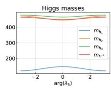
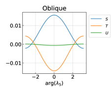
Figure 2: Higgs boson masses(left) and oblique parameters (right) for the parameter point in eq. (5) as a function of the phase of $\lambda_{5}$.

Varying arg$\lambda_{5}$ has a large effect on the oblique parameters $S$, $T$ and $U$, as can be seen in the right plot in figure 2. In figure 3, it is shown how a non-zero phase quickly induces a large EDM, $d_{e}$, for the electron. There can be non-trivial cancellations among the many contributions to $d_{e}$; with the lightest Higgs boson usually dominating. Including the $(d_{e})^{\gamma h_{2,3}}$ diagram is however important since it is at the same order of magnitude.

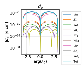
Figure 3: The eEDM as a function of arg$\lambda_{5}$ for the parameter point in eq. (5). The different contributions, $VS$, refers to the individual Barr-Zee diagrams, as in figure 4, summed over all different loop particles.

In figure 4 we show the branching ratios of the Higgs bosons as a function of arg$\lambda_{5}$. There are a number of new possible decays opening up when going to a $\mathcal{CP}$ violating 2HDM since the neutral Higgs bosons all mix together. For example, one can have $h_{2}$ and $h_{3}$ simultaneously decaying into $Zh_{1}$ as well as to $h_{1}h_{1}$.

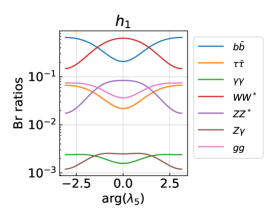
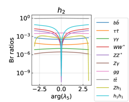
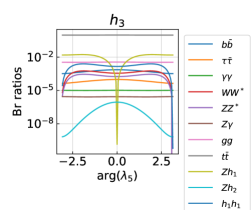
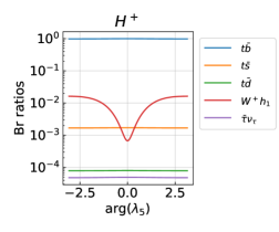
Figure 4: Branching ratios for the most important decays of the Higgs particles.

6 Results

In the parameter scan, we perform the RG evolution from the top mass scale until the evolution breaks down. We define the energy scale $\Lambda$ as the breakdown energy scale; meaning the energy where either perturbativity, stability or unitarity is violated.

If nothing else if mentioned, the figures presented below are constructed from the parameter points that are allowed by HiggsBounds and HiggsSignals as well as within the limits of $S$, $T$ and $U$.

Scenario	$\mathbb{Z}_{2}$	Pass HB	Pass HS	Pass ST	Pass eEDM	Pass all
I	type I	43%	9%	80%	9%	1.3%
I	type II	39%	7%	80%	6%	0.5%
II	type I	38%	8%	74%	5%	0.7%
II	type II	36%	6%	74%	2%	0.2%
III	type I	44%	9%	80%	3%	0.4%
III	type II	44%	8%	79%	1%	0.01%
III	type X	43%	8%	79%	1%	0.01%

Table 2: Statistics of the parameter scans of scenario I-III. HB (HS) refers to HiggsBounds (HiggSignals). There is a total of 50 000 points in each scenario. The $\mathbb{Z}_{2}$ symmetry for scenario III sets the magnitude for the complex $a_{F}$ coefficients.

The fraction of points that survives the different constraints at the starting scale of the parameter scans is shown in table 2 for all the scenarios. In table 3, we also list the three largest contributions to the eEDM.

Scenario	$\mathbb{Z}_{2}$	1st	2nd	3rd
I	type I	$\gamma h_{1}(W)$: 85 %	$\gamma h_{2}(W)$: 10 %	$\gamma h_{2}(t)$: 3 %
I	type II	$\gamma h_{1}(W)$: 60 %	$\gamma h_{1}(t)$: 24 %	$\gamma h_{2}(t)$: 5 %
II	type I	$\gamma h_{1}(W)$: 79 %	$\gamma h_{2}(W)$: 12 %	$\gamma h_{2}(t)$: 5 %
II	type II	$\gamma h_{1}(W)$: 58 %	$\gamma h_{1}(t)$: 20 %	$\gamma h_{2}(t)$: 11 %
III	type I	$\gamma h_{2}(t)$: 31 %	$\gamma h_{3}(t)$: 22 %	$\gamma h_{1}(W)$: 19 %
III	type II	$\gamma h_{2}(t)$: 31 %	$\gamma h_{1}(W)$: 25 %	$\gamma h_{3}(t)$: 22 %
III	type X	$\gamma h_{2}(t)$: 31 %	$\gamma h_{2}(W)$: 25 %	$\gamma h_{3}(t)$: 23 %

Table 3: Statistics of the top three largest contributions to the eEDM for all 50 000 parameter points in each scenario. The notation is according to figure 4, i.e. $VS$(loop particle).

6.1 Scenario I

Scenario I
type I type II

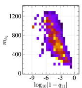
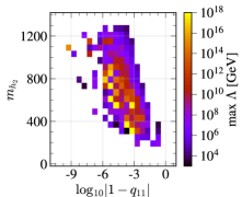
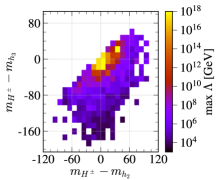
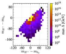
Figure 5: The maximum breakdown energy $\Lambda$ as a function of masses, mass differences and the $q_{11}$ parameter for type I (left) and type II (right).

Scenario I
type I type II

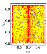
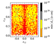
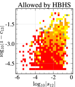
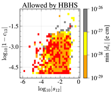
Figure 6: The minimum eEDM as a function of the angles $s_{12}$ and $c_{13}$ for type I (left) and type II (right). The top figures are all parameter points, while the bottom figures contain only points allowed by HiggsBounds and HiggsSignals. Red denotes eEDM below $10^{-29}$ e cm.

Scenario I
type I type II

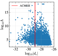
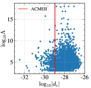
Figure 7: The relation between breakdown energy and eEDM for type I (left) and type II (right). The red line is the ACMEII eEDM limit, $1.1\times 10^{-29}$ e cm.

Scenario I
type I type II

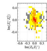
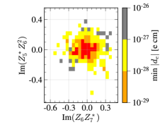
Figure 8: The minimum eEDM as a function of the base invariant quantities $Z_{5}^{*}Z_{6}^{2}$ and $Z_{6}^{*}Z_{7}$ for type I (left) and type II (right).

Scenario I
type I type II

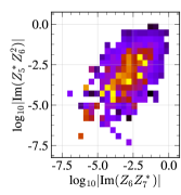
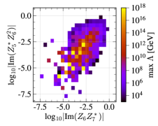
Figure 9: The maximum breakdown energy as a function of the base invariant quantities $Z_{5}^{*}Z_{6}^{2}$ and $Z_{6}^{*}Z_{7}$ for type I (left) and type II (right).

Because of the small quartic couplings, the mass spectrum falls easily into an aligned scenario with $q_{11}\sim 1$. It is easy to find parameter points with heavy $h_{2,3}$ and $H^{\pm}$ as can be seen in figure 5; however, heavier masses implies that the model is more aligned, i.e. $q_{11}$ goes to 1 as the masses increase. In the figure, the maximum breakdown energy in each bin is shown as a function of the masses, mass differences as well as $q_{11}$. From the figure, it is also clear that only models with small mass differences between the heavy Higgses can be evolved to high scales. There is also a preference for $q_{11}$ being very close to 1.

The general property that only very aligned models are viable at the starting scale is because these are the only ones allowed by HiggsBounds and HiggsSignals. To illustrate this, we show the eEDM as a function of the angles $s_{12}$ and $c_{13}$ in figure 6. There, two figures for each Yukawa symmetry are displayed: one before running the parameter points through HiggsBounds and HiggsSignals and one with only the points allowed by these programs. The allowed points with a small eEDM all fall in the aligned region of $s_{12}\sim 0$ and $c_{13}\sim 1$.

To see if a small eEDM also implies a 2HDM that can be evolved to high energies, we show a scatter plot of the breakdown energy and eEDM in figure 7. As can be seen from the figure, this is not the case; there is no definite correlation saying that small eEDM gives a high $\Lambda$. Most points have a too high eEDM and points that are valid up to the Planck scale exist, presumably, in the entire region.

Even though there is only one phase in scenario I, $\arg\lambda_{5}$, that is the source of $\mathcal{CP}$ violation in the scalar potential, we find that the base invariant quantities in eq. (62) are better measures of the amount of $\mathcal{CP}$ violation in the 2HDM. This is because they are also dependent on $\tan\beta$ and other quartic couplings that for example also influence the eEDM; in addition, it also simplifies the comparison between different scenarios. All parameter points that pass the ACMEII bound have these quantities at the order of $0.1$. The eEDM as a function of Im$(Z_{5}^{*}Z_{6}^{2})$ and Im$(Z_{6}^{*}Z_{7})$ is shown in figure 8. In figure 9, we show the maximum breakdown energy as a function of the same $\mathcal{CP}$ violating quantities and there one can see that all parameter points that are valid all the way to the Planck scale have Im$(Z_{5}^{*}Z_{6}^{2})\sim$Im$(Z_{6}^{*}Z_{7})\sim 10^{-2}$, thus constraining these parameters even further.

6.2 Scenario II

Scenario II
type I type II

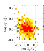
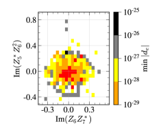
Figure 10: The minimum eEDM as a function of the base invariant quantities $Z_{5}^{*}Z_{6}^{2}$ and $Z_{6}^{*}Z_{7}$ for type I (left) and type II (right).

The results of scenario II are largely following that of scenario I; one gets the same mass spectrum characteristics and the parameter points that survive are aligned in a similar way as in figure 5. The addition of non-zero $\lambda_{6,7}$ parameters does, however, have some effects.

We first note that base-invariant quantities $Z_{5}^{*}Z_{6}^{2}$ and $Z_{6}^{*}Z_{7}$ get additional contributions from $\lambda_{6}$ and $\lambda_{7}$. In figure 10 we see that this increases the allowed range of the imaginary parts of these quantities, while still having an allowed eEDM.

Scenario II
type I type II

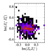
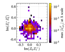
Figure 11: The maximum induced non-diagonal Yukawa element in the Cheng-Sher parameterization as a function of the base invariant quantities $Z_{5}^{*}Z_{6}^{2}$ and $Z_{6}^{*}Z_{7}$ for type I (left) and type II (right).

Scenario II
type I type II

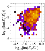
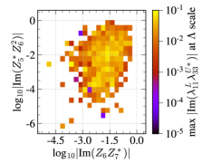
Figure 12: The maximum induced imaginary part of $\lambda_{33}^{L}\lambda_{33}^{U*}$ at the breakdown energy scale as a function of the base invariant quantities $Z_{5}^{*}Z_{6}^{2}$ and $Z_{6}^{*}Z_{7}$ for type I (left) and type II (right).

Since the $\lambda_{6,7}$ parameters break the $\mathbb{Z}_{2}$ symmetry hard, the symmetry breaking spreads in the RG running to the Yukawa sector as well. This does not have a huge impact, however, since the quartic couplings enter the Yukawa couplings RGEs first at 2-loop order. The maximum induced non-diagonal Yukawa coupling as a function of the imaginary parts of $Z_{5}^{*}Z_{6}^{2}$ and $Z_{6}^{*}Z_{7}$ is shown in figure 11. There we see that although the effect is much larger with a type II Yukawa sector, one does not get size-able FCNCs after RG running. For type I (type II) the maximum generated non-diagonal Yukawa element is $\lambda_{i\neq j}^{F}\sim 10^{-3}(10^{-2})$ at the breakdown energy scale. Similar findings are presented in ref. Oredsson:2018yho in the $\mathcal{CP}$ conserving case. In this $\mathcal{CP}$ violating case, one can generate a non-trivial amount of $\mathcal{CP}$ violation in the Yukawa sector though. To see this, we show the maximum generated imaginary part of the base invariant quantity $\lambda_{11}^{L}\lambda_{33}^{U*}$ in figure 12. This parameter is chosen because it needs to be small to not yield a too large eEDM; as is discussed in scenario III.

Scenario II
type I type II

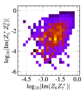
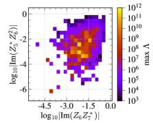
Figure 13: The maximum breakdown energy as a function of the base invariant quantities $Z_{5}^{*}Z_{6}^{2}$ and $Z_{6}^{*}Z_{7}$ for type I (left) and type II (right).

The imaginary parts of $Z_{5}^{*}Z_{6}^{2}$ and $Z_{6}^{*}Z_{7}$ serves as good measures of the amount of $\mathcal{CP}$ violation in the 2HDM as seen in figure 10; all the points that satisfy the eEDM bound are centered around them being zero. The parameter points that are valid up to the highest energies also exhibit small Im$(Z_{5}^{*}Z_{6}^{2})$ and Im$(Z_{6}^{*}Z_{7})$ as can be seen in figure 13.

6.3 Scenario III

Scenario III
type I type II type X

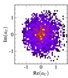
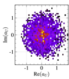
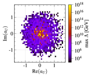
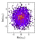
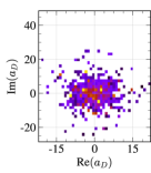
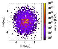
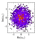
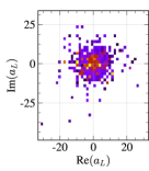
Figure 14: The maximum breakdown energy as a function of $a_{U}$, $a_{D}$ and $a_{L}$ for type I (left), type II (middle) and type X (right).

Scenario III
type I type II type X

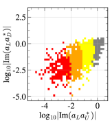
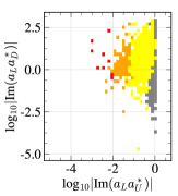
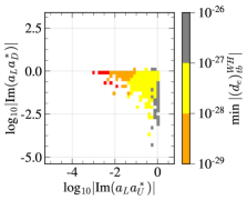
Figure 15: The minimum contribution from $(d_{e})^{WH}_{tb}$ to the eEDM as a function of the imaginary parts of $a_{L}a_{U}^{*}$ and $a_{L}a_{D}^{*}$ for type I (left), type II (middle) and type X (right).

Scenario III
type I type II type X

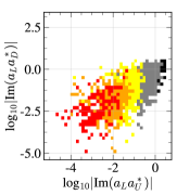
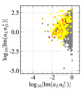
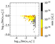
Figure 16: The minimum eEDM as a function of the imaginary parts of $a_{L}a_{U}^{*}$ and $a_{L}a_{D}^{*}$ for type I (left), type II (middle) and type X (right).

Scenario III
type I type II type X

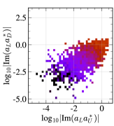
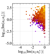
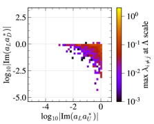
Figure 17: The maximum induced non-diagonal Yukawa couplings in the Cheng-Sher ansatz as a function of the imaginary parts of $a_{L}a_{U}^{*}$ and $a_{L}a_{D}^{*}$ for type I (left), type II (middle) and type X (right).

Scenario III
type I type II type X

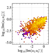
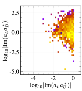
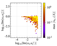
Figure 18: The maximum induced hard $\mathbb{Z}_{2}$ symmetry breaking parameters $\lambda_{6,7}$ as a function of the imaginary parts of $a_{L}a_{U}^{*}$ and $a_{L}a_{D}^{*}$ for type I (left), type II (middle) and type X (right).

Scenario III
type I type II type X

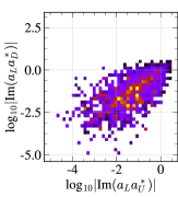
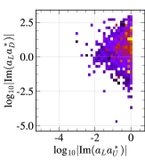
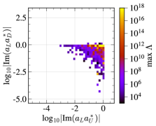
Figure 19: The maximum breakdown energy as a function of the imaginary parts of $a_{L}a_{U}^{*}$ and $a_{L}a_{D}^{*}$ for type I (left), type II (middle) and type X (right).

The maximum breakdown energy as function of the aligned coefficients $a_{F}$ is shown in figure 14 for the three different types. The results are largely independent on the phase of each $a_{F}$, while the regions around zero tend to be better for higher breakdown energies. For type I, this means that $\tan\beta$ has to be quite large since $|a_{F}|=1/\tan\beta$, whereas for type II and X there is a balance between $|a_{U}|=1/\tan\beta$ being small and at the same time $|a_{D}|=\tan\beta$ and/or $|a_{L}|=\tan\beta$ not being too large ($\lesssim 10$).

As measure of the $\mathcal{CP}$ violation, we use the base invariant quantities Im$(a_{L}a_{U}^{*})$ and Im$(a_{L}a_{D}^{*})$. These give the contribution $(d_{e})^{WH}_{tb}$ in eq. (B); which is the largest contribution in $\sim 10$ % of the parameter points. The term involving $a_{U}$ is the dominant one because of the top mass and therefore one gets a very clear limit on Im$(a_{L}a_{U}^{*})$ as can be seen in figure 15, where the single contribution $(d_{e})^{WH}_{tb}$ is shown as a function of Im$(a_{L}a_{U}^{*})$ and Im$(a_{L}a_{D}^{*})$. There, the Im$(a_{L}a_{U}^{*})$ needs to be below $\sim 0.01$ for all types to be within the limits of ACMEII. In figure 16 we show the total eEDM as a function of the same parameters. Although, there are some cancellations that make the limit on Im$(a_{L}a_{U}^{*})$ fuzzier, the eEDM still gives quite a severe constraint; especially for type I, although for type II and X we are facing the problem of running out of statistics. For type II and X there are some points with large Im$(a_{L}a_{U}^{*})$ and Im$(a_{L}a_{D}^{*})$ that still give an allowed eEDM. There could even be regions for these last types that could pass all constraints and still be valid all the way to the Planck scale; although this requires more study.

Breaking the $\mathbb{Z}_{2}$ symmetry in the Yukawa sector can give rise to non-diagonal Yukawa couplings. In figure 17, this is shown as a function of Im$(a_{L}a_{U}^{*})$ and Im$(a_{L}a_{D}^{*})$. Similarly as in scenario II, type II is generating the most FCNCs in the RG evolution. The regions in type I that are within the eEDM limits generate a very low amount of FCNCs.

The hard $\mathbb{Z}_{2}$ symmetry breaking quartic couplings $\lambda_{6,7}$ are also generated in general; as seen in figure 18, where max$(\lambda_{6,7})$ as a function of Im$(a_{L}a_{U}^{*})$ and Im$(a_{L}a_{D}^{*})$ is plotted. All scenarios generate size-able $\lambda_{6,7}$ easily.

7 Conclusions

We have analyzed the $\mathcal{CP}$ violating 2HDM by performing numerical parameter scans in three different physical scenarios. Using 2HDME, we have performed 2-loop RG running to study the properties under RG evolution looking for Landau poles as well as a breakdown of unitarity or stability. Experimental collider data has been used to restrict the parameter space with the codes HiggsBounds and HiggsSignals and we also checked the oblique parameters $S$, $T$ and $U$. The amount of $\mathcal{CP}$ violation was constrained by calculating the eEDM; which now is an implemented feature of 2HDME.

The physical scenarios we have investigated start from a 2HDM with a softly broken $\mathbb{Z}_{2}$ symmetry and quartic couplings $|\lambda_{i}|\leq 2$, to which we add additional sources of (hard) $\mathbb{Z}_{2}$ breaking.

With a softly broken $\mathbb{Z}_{2}$ symmetry and $\mathcal{CP}$ violation in the scalar potential, we found that having $|\lambda_{i}|\leq 2$ gives an aligned 2HDM with the alignment parameter $q_{11}\rightarrow 1$ as the BSM Higgs masses become heavy. We also find that the amount of $\mathcal{CP}$ violation is severely constrained by the eEDM. The limit from ACMEII requires the base invariant quantities Im$(Z_{5}^{*}Z_{6}^{2})$ and Im$(Z_{6}Z_{7}^{*})$ to be $\sim 0.1$ for parameter points to be allowed. For the points that are valid up to the Planck scale, these quantities are even further constrained, $\sim 0.01$.

We also investigated the complex 2HDM with a small hard breaking of the $\mathbb{Z}_{2}$ symmetry in the scalar potential by having non-zero $\lambda_{6,7}$ at the EW scale. While finding similar findings as the softly broken symmetry case, one also gets the effect of inducing a $\mathbb{Z}_{2}$ symmetry breaking in the Yukawa sector during the RG running. Although, we found that there are no sizeable FCNCs being produced, the $\mathcal{CP}$ violation in the scalar sector can spread to the Yukawa sector by a non-trivial amount.

Lastly, we investigated three scenarios of aligned Yukawa sector based on type I, II and X, but with complex coefficients. For the type I based scenario, we find that it is severely constrained by the eEDM, which requires Im$(a_{L}a_{U}^{*})\lesssim 10^{-2}$. This is most easily satisfied if $\tan\beta$ is large. For the type II and X based scenarios, the constraint on Im$(a_{L}a_{U}^{*})$ tends to be weaker due to cancellations between different contributions to the eEDM. At the same time, these scenarios are in general much worse than that of type I. During RG running, the symmetry breaking spreads to the scalar sector and induces complex $\lambda_{6,7}$ as well as FCNCs. The FCNCs are, however, not very large for parameter points that have an allowed eEDM.

Appendix A Generic basis in scenario I

Scenario I

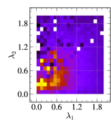
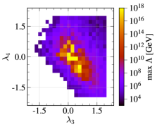
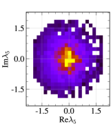
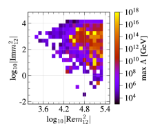
Figure 20: The maximum breakdown energy as a function of the parameters in the generic basis in scenario I with a type I $\mathbb{Z}_{2}$ symmetry.

The parameter scans are generating the scalar potential in the generic basis with flat random distributions. The breakdown energy scale as a function of the quartic couplings and $m_{12}^{2}$ is shown in figure 20.

Appendix B Barr-Zee diagrams for EDM

The largest contributions to light fermions’ EDM comes from 2-loop Barr-Zee diagrams Barr:1990vd , as shown in figure 4. The computation of these diagrams in the context of the 2HDM was first done in ref. Chang:1990sf . A general framework to compute them is presented in ref. Nakai:2016atk . The results for the 2HDM can be found in various sources, e.g. ref. Inoue:2014nva . Most of the literature, however, deal with a softly broken $\mathbb{Z}_{2}$ symmetry. We found that these results are incomplete, e.g. when investigating the 2HDM with a complex aligned Yukawa sector, and therefore compliment the EDM computation with diagrams involving $W^{\pm},H^{\pm}$ and a fermion loop. This additional contribution as well as all other contributions, for completeness, are presented below.

We denote each contribution to the electrons EDM as

$$(d_{e})^{VS}_{l},$$ (65)

where $l$ denotes the particles of the 1-loop blob in figure 4. Although some formulas below are written for a general loop particle, diagrams with light particles participating in the loops are very suppressed. Therefore we only include the third generation in the total electron EDM; which then reduces to

$$d_{e}=\sum_{h}\left\{\sum_{f=t,b,\tau}\left[(d_{e})^{\gamma h}_{f}+(d_{e})^{Zh}_{f}\right]+(d_{e})^{\gamma h}_{W}+(d_{e})^{\gamma h}_{H}+(d_{e})^{Zh}_{H}+(d_{e})_{hH}^{WH}\right\}+(d_{e})^{WH}_{tb},$$ (66)

where $H$ denotes the charged Higgs.

The tree-level Higgs masses vary with renormalization scale. To circumvent this, we always use the Higgs mass which satisfies $m_{h}(\mu)=\mu$, which is independent on renormalization scale.

All the couplings in each contribution are defined at the mass scale of the heaviest particle participating in the loop diagram and we use full 2-loop RGEs to run between the energy scales. The theoretical uncertainty in the calculation is rather high since the running of couplings change some quantities rather dramatically and the choice of renormalization scale for each diagram is somewhat arbitrary. To get an estimate, we varied the renormalization scale for each diagram to be twice or half the highest participating mass in the loop, which can change $d_{e}$ by a factor of 2. This is, however, good enough for any conclusions we make in this work.

Fermion loops

For each fermion $f$, the contribution to the electrons EDM is

$$(d_{e})^{\gamma h}_{f}=~{} \frac{N_{c}Q_{f}^{2}e^{3}}{32\pi^{4}m_{f}}\times\sum_{k=1}^{3}\left[f(z_{f}^{k})(c_{k}^{F})_{ff}(\tilde{c}_{k}^{L})_{ee}+g(z_{f}^{k})(\tilde{c}_{k}^{F})_{ff}(c_{k}^{L})_{ee}\right],$$ (67)

where the loop functions are listed at the end of this section. We define the ratio of masses as $z_{x}^{k}\equiv m_{x}^{2}/m_{h_{k}}^{2}$.

The similar diagram with a $Z$ boson instead of the internal $\gamma$ is

$$(d_{e})^{Zh}_{f}=~{} \frac{N_{c}eg_{Zee}^{V}g_{Zff}^{V}}{32\pi^{4}m_{f}}\times\sum_{k=1}^{3}\left[\tilde{f}(z_{f}^{k},m_{f}^{2}/m_{Z}^{2})(c_{k}^{F})_{ff}(\tilde{c}_{k}^{L})_{ee}+\tilde{g}(z_{f}^{k},m_{f}^{2}/m_{Z}^{2})(\tilde{c}_{k}^{F})_{ff}(c_{k}^{L})_{ee}\right],$$ (68)

where $g_{Zff}^{V}=g(T_{3}^{f}-2Q_{f}\sin^{2}\theta_{W})/(2\cos\theta_{W})$.

For a general Yukawa sector, there is also an important contribution coming from a $W^{\pm}-H^{\pm}$ diagram with a fermion loop. This single contribution is investigated in ref. BowserChao:1997bb , where they only keep the term proportional $\rho^{U}$. We have computed this again with the framework in ref. Nakai:2016atk and kept also the $\rho^{D}$ term. The result for the third generation fermions is

$$(d_{e})^{WH}_{tb}=~{} \frac{N_{c}e^{3}|(V_{CKM})_{tb}|^{2}}{512\pi^{4}\sin^{2}\theta_{W}(m_{H^{\pm}}^{2}-m_{W}^{2})}\int_{0}^{1}\mathrm{d}x\left[Q_{t}x+Q_{b}(1-x)\right]$$

$$\times\left\{\text{Im}\left[(\rho^{L})_{ee}(\rho^{U})^{*}_{tt}\right]m_{t}x(1+x)+\text{Im}\left[(\rho^{L})_{ee}(\rho^{D})^{*}_{bb}\right]m_{b}x(1-x)\right\}$$

$$\times\left[G\left(\frac{m_{t}^{2}}{m_{H^{\pm}}^{2}},\frac{m_{b}^{2}}{m_{H^{\pm}}^{2}}\right)-G\left(\frac{m_{t}^{2}}{m_{W}^{2}},\frac{m_{b}^{2}}{m_{W}^{2}}\right)\right].$$ (69)

This is the same formula as one gets for the case of magnetic dipole moment, derived in ref. Ilisie:2015tra ; except that it is the imaginary part of the couplings instead of the real part.

$W$ loops

With a $W$ internal gauge boson, one gets the contributions

$$(d_{e})^{\gamma h}_{W}=~{} -\frac{e^{3}}{128\pi^{4}v}\sum_{k=1}^{3}\left[\left(6+\frac{1}{z_{W}^{k}}\right)f(z_{W}^{k})+\left(10-\frac{1}{z_{W}^{k}}\right)g(z_{W}^{k})\right]g_{kVV}(\tilde{c}_{k}^{L})_{ee}.$$ (70)

and

$$(d_{e})^{Zh}_{W}=~{} \frac{eg_{ZWW}g_{Zee}^{V}}{128\pi^{4}v}\sum_{k=1}^{3}\left[\left(6-\text{sec}^{2}\theta_{W}+\frac{2-\text{sec}^{2}\theta_{W}}{2z_{W}^{k}}\right)\tilde{f}(z_{W}^{k},\cos^{2}\theta_{W})\right.$$

$$\left.+\left(10-3\text{sec}^{2}\theta_{W}-\frac{2-\text{sec}^{2}\theta_{W}}{2z_{W}^{k}}\right)\tilde{g}(z_{W}^{k},\cos^{2}\theta_{W})\right]g_{kVV}(\tilde{c}_{k}^{L})_{ee},$$ (71)

where $g_{ZWW}\equiv e\cot\theta_{W}$.

Scalar loops

The charged scalar contribution is

$$(d_{e})^{\gamma h}_{H}=~{} -\frac{e^{3}v}{128\pi^{4}m_{H^{\pm}}^{2}}\sum_{k=1}^{3}\left[f(z_{H}^{k})-g(z_{H}^{k})\right]\lambda_{kH^{\pm}}(\tilde{c}_{k}^{L})_{ee}$$ (72)

and

$$(d_{e})^{Zh}_{H}=~{} -\frac{evg_{Zee}^{V}g_{ZH^{\pm}}}{128\pi^{4}m_{H^{\pm}}^{2}}\sum_{k=1}^{3}\left[\tilde{f}(z_{H}^{k},m_{H^{\pm}}^{2}/m_{Z}^{2})-\tilde{g}(z_{H}^{k},m_{H^{\pm}}^{2}/m_{Z}^{2})\right]\lambda_{kH^{\pm}}(\tilde{c}_{k}^{L})_{ee},$$ (73)

where $g_{ZH^{\pm}}\equiv e\cot\theta_{W}(1-\tan^{2}\theta_{W})/2$.

The gauge invariant contribution from charged and neutral scalars has been calculated in ref. Abe:2013qla ,

$$(d_{e})_{hH}^{WH}=~{} \frac{e}{256\pi^{4}v}\times\sum_{k=1}^{3}\left[\frac{e^{2}}{2\sin^{2}\theta_{W}}\mathcal{I}_{4}(m_{h_{k}}^{2},m_{H^{\pm}}^{2})g_{kVV}-\mathcal{I}_{5}(m_{h_{k}}^{2},m_{H^{\pm}}^{2})\lambda_{kH^{\pm}}\right](\tilde{c}_{k}^{L})_{ee}.$$ (74)

Miscellaneous functions

$$f(z)=~{} \frac{z}{2}\int_{0}^{1}\mathrm{d}x\frac{1-2x(1-x)}{x(1-x)-z}\log\left(\frac{x(1-x)}{z}\right),$$ (75)

$$g(z)=~{} \frac{z}{2}\int_{0}^{1}\mathrm{d}x\frac{1}{x(1-x)-z}\log\left(\frac{x(1-x)}{z}\right),$$ (76)

$$\tilde{f}(x,y)=~{} \frac{yf(x)}{y-x}+\frac{xf(y)}{x-y},$$ (77)

$$\tilde{g}(x,y)=~{} \frac{yg(x)}{y-x}+\frac{xg(y)}{x-y},$$ (78)

$$G(r_{1},r_{2})=\frac{\log\left(\frac{r_{1}x+r_{2}(1-x)}{x(1-x)}\right)}{x(1-x)-r_{1}x-r_{2}(1-x)},$$ (79)

$$\mathcal{I}_{4,5}(m_{1}^{2},m_{2}^{2})=~{} \frac{m_{W}^{2}}{m_{H^{\pm}}^{2}-m_{W}^{2}}\left[I_{4,5}(m_{W}^{2},m_{1}^{2})-I_{4,5}(m_{2}^{2},m_{1}^{2})\right],$$ (80)

$$I_{4}(m_{1}^{2},m_{2}^{2})=~{} \int_{0}^{1}\mathrm{d}z(1-z)^{2}\left(z-4+z\frac{m_{H^{\pm}}^{2}-m_{2}^{2}}{m_{W}^{2}}\right)$$

$$\times\frac{m_{1}^{2}}{m_{W}^{2}(1-z)+m_{2}^{2}z-m_{1}^{2}z(1-z)}\log\left(\frac{m_{W}^{2}(1-z)+m_{2}^{2}z}{m_{1}^{2}z(1-z)}\right),$$ (81)

$$I_{5}(m_{1}^{2},m_{2}^{2})=~{} \int_{0}^{1}\mathrm{d}z\frac{m_{1}^{2}z(1-z)^{2}}{m_{W}^{2}(1-z)+m_{2}^{2}z-m_{1}^{2}z(1-z)}\log\left(\frac{m_{W}^{2}(1-z)+m_{2}^{2}z}{m_{1}^{2}z(1-z)}\right).$$ (82)

References

- (1) ATLAS Collaboration, G. Aad et. al., Observation of a new particle in the search for the Standard Model Higgs boson with the ATLAS detector at the LHC, Phys. Lett. B716 (2012) 1–29, [arXiv:1207.7214].
- (2) CMS Collaboration, S. Chatrchyan et. al., Observation of a new boson at a mass of 125 GeV with the CMS experiment at the LHC, Phys. Lett. B716 (2012) 30–61, [arXiv:1207.7235].
- (3) ATLAS, CMS Collaboration, G. Aad et. al., Measurements of the Higgs boson production and decay rates and constraints on its couplings from a combined ATLAS and CMS analysis of the LHC pp collision data at and 8 TeV, JHEP 08 (2016) 045, [arXiv:1606.02266].
- (4) CMS Collaboration, V. Khachatryan et. al., Constraints on the spin-parity and anomalous HVV couplings of the Higgs boson in proton collisions at 7 and 8 TeV, Phys. Rev. D92 (2015), no. 1 012004, [arXiv:1411.3441].
- (5) A. D. Sakharov, Violation of CP Invariance, C asymmetry, and baryon asymmetry of the universe, Pisma Zh. Eksp. Teor. Fiz. 5 (1967) 32–35. [Usp. Fiz. Nauk161,no.5,61(1991)].
- (6) T. D. Lee, A Theory of Spontaneous T Violation, Phys. Rev. D8 (1973) 1226–1239. [,516(1973)].
- (7) ACME Collaboration, V. Andreev et. al., Improved limit on the electric dipole moment of the electron, Nature 562 (2018), no. 7727 355–360.
- (8) S. L. Glashow and S. Weinberg, Natural Conservation Laws for Neutral Currents, Phys. Rev. D15 (1977) 1958.
- (9) E. A. Paschos, Diagonal Neutral Currents, Phys. Rev. D15 (1977) 1966.
- (10) J. Shu and Y. Zhang, Impact of a CP Violating Higgs Sector: From LHC to Baryogenesis, Phys. Rev. Lett. 111 (2013), no. 9 091801, [arXiv:1304.0773].
- (11) M. Jung and A. Pich, Electric Dipole Moments in Two-Higgs-Doublet Models, JHEP 04 (2014) 076, [arXiv:1308.6283].
- (12) S. Inoue, M. J. Ramsey-Musolf, and Y. Zhang, CP-violating phenomenology of flavor conserving two Higgs doublet models, Phys. Rev. D89 (2014), no. 11 115023, [arXiv:1403.4257].
- (13) K. Cheung, J. S. Lee, E. Senaha, and P.-Y. Tseng, Confronting Higgcision with Electric Dipole Moments, JHEP 06 (2014) 149, [arXiv:1403.4775].
- (14) S. Ipek, Perturbative analysis of the electron electric dipole moment and CP violation in two-Higgs-doublet models, Phys. Rev. D89 (2014), no. 7 073012, [arXiv:1310.6790].
- (15) L. Bian, T. Liu, and J. Shu, Cancellations Between Two-Loop Contributions to the Electron Electric Dipole Moment with a CP-Violating Higgs Sector, Phys. Rev. Lett. 115 (2015) 021801, [arXiv:1411.6695].
- (16) C.-Y. Chen, S. Dawson, and Y. Zhang, Complementarity of LHC and EDMs for Exploring Higgs CP Violation, JHEP 06 (2015) 056, [arXiv:1503.01114].
- (17) D. Fontes, M. Mühlleitner, J. C. Romão, R. Santos, J. P. Silva, and J. Wittbrodt, The C2HDM revisited, JHEP 02 (2018) 073, [arXiv:1711.09419].
- (18) D. Egana-Ugrinovic and S. Thomas, Higgs Boson Contributions to the Electron Electric Dipole Moment, arXiv:1810.08631.
- (19) P. S. Bhupal Dev and A. Pilaftsis, Maximally Symmetric Two Higgs Doublet Model with Natural Standard Model Alignment, JHEP 12 (2014) 024, [arXiv:1408.3405]. [Erratum: JHEP11,147(2015)].
- (20) A. Peñuelas and A. Pich, Flavour alignment in multi-Higgs-doublet models, JHEP 12 (2017) 084, [arXiv:1710.02040].
- (21) F. J. Botella, F. Cornet-Gomez, and M. Nebot, Flavour Conservation in Two Higgs Doublet Models, arXiv:1803.08521.
- (22) S. Gori, H. E. Haber, and E. Santos, High scale flavor alignment in two-Higgs doublet models and its phenomenology, JHEP 06 (2017) 110, [arXiv:1703.05873].
- (23) P. Basler, P. M. Ferreira, M. Mühlleitner, and R. Santos, High scale impact in alignment and decoupling in two-Higgs doublet models, Phys. Rev. D97 (2018), no. 9 095024, [arXiv:1710.10410].
- (24) P. Ferreira, H. E. Haber, and E. Santos, Preserving the validity of the Two-Higgs Doublet Model up to the Planck scale, Phys. Rev. D92 (2015) 033003, [arXiv:1505.04001]. [Erratum: Phys. Rev.D94,no.5,059903(2016)].
- (25) J. Bijnens, J. Lu, and J. Rathsman, Constraining General Two Higgs Doublet Models by the Evolution of Yukawa Couplings, JHEP 1205 (2012) 118, [arXiv:1111.5760].
- (26) D. Chowdhury and O. Eberhardt, Global fits of the two-loop renormalized Two-Higgs-Doublet model with soft Z2 breaking, JHEP 11 (2015) 052, [arXiv:1503.08216].
- (27) M. E. Krauss, T. Opferkuch, and F. Staub, The Ultraviolet Landscape of Two-Higgs Doublet Models, arXiv:1807.07581.
- (28) J. Oredsson and J. Rathsman, breaking effects in 2-loop RG evolution of 2HDM, JHEP 02 (2019) 152, [arXiv:1810.02588].
- (29) J. Oredsson, 2 Higgs Doublet Model Evolver - Manual, arXiv:1811.08215.
- (30) D. Eriksson, J. Rathsman, and O. Stål, 2HDMC: Two-Higgs-Doublet Model Calculator Physics and Manual, Comput. Phys. Commun. 181 (2010) 189–205, [arXiv:0902.0851].
- (31) P. Bechtle, O. Brein, S. Heinemeyer, G. Weiglein, and K. E. Williams, HiggsBounds: Confronting Arbitrary Higgs Sectors with Exclusion Bounds from LEP and the Tevatron, Comput. Phys. Commun. 181 (2010) 138–167, [arXiv:0811.4169].
- (32) P. Bechtle, O. Brein, S. Heinemeyer, G. Weiglein, and K. E. Williams, HiggsBounds 2.0.0: Confronting Neutral and Charged Higgs Sector Predictions with Exclusion Bounds from LEP and the Tevatron, Comput. Phys. Commun. 182 (2011) 2605–2631, [arXiv:1102.1898].
- (33) P. Bechtle, O. Brein, S. Heinemeyer, O. Stål, T. Stefaniak, G. Weiglein, and K. E. Williams, : Improved Tests of Extended Higgs Sectors against Exclusion Bounds from LEP, the Tevatron and the LHC, Eur. Phys. J. C74 (2014), no. 3 2693, [arXiv:1311.0055].
- (34) P. Bechtle, S. Heinemeyer, O. Stål, T. Stefaniak, and G. Weiglein, : Confronting arbitrary Higgs sectors with measurements at the Tevatron and the LHC, Eur. Phys. J. C74 (2014), no. 2 2711, [arXiv:1305.1933].
- (35) S. M. Barr and A. Zee, Electric Dipole Moment of the Electron and of the Neutron, Phys. Rev. Lett. 65 (1990) 21–24. [Erratum: Phys. Rev. Lett.65,2920(1990)].
- (36) G. Branco, P. Ferreira, L. Lavoura, M. Rebelo, M. Sher, et. al., Theory and phenomenology of two-Higgs-doublet models, Phys.Rept. 516 (2012) 1–102, [arXiv:1106.0034].
- (37) S. Davidson and H. E. Haber, Basis-independent methods for the two-Higgs-doublet model, Phys. Rev. D72 (2005) 035004, [hep-ph/0504050]. [Erratum: Phys. Rev.D72,099902(2005)].
- (38) H. E. Haber and D. O’Neil, Basis-independent methods for the two-Higgs-doublet model. II. The Significance of tan, Phys. Rev. D74 (2006) 015018, [hep-ph/0602242]. [Erratum: Phys. Rev.D74,no.5,059905(2006)].
- (39) H. E. Haber and D. O’Neil, Basis-independent methods for the two-Higgs-doublet model III: The CP-conserving limit, custodial symmetry, and the oblique parameters S, T, U, Phys. Rev. D83 (2011) 055017, [arXiv:1011.6188].
- (40) G. C. Branco, L. Lavoura, and J. P. Silva, CP Violation, Int. Ser. Monogr. Phys. 103 (1999) 1–536.
- (41) A. Pich and P. Tuzon, Yukawa Alignment in the Two-Higgs-Doublet Model, Phys. Rev. D80 (2009) 091702, [arXiv:0908.1554].
- (42) M. Jung, A. Pich, and P. Tuzon, Charged-Higgs phenomenology in the Aligned two-Higgs-doublet model, JHEP 11 (2010) 003, [arXiv:1006.0470].
- (43) P. M. Ferreira, L. Lavoura, and J. P. Silva, Renormalization-group constraints on Yukawa alignment in multi-Higgs-doublet models, Phys. Lett. B688 (2010) 341–344, [arXiv:1001.2561].
- (44) F. J. Botella, G. C. Branco, A. M. Coutinho, M. N. Rebelo, and J. I. Silva-Marcos, Natural Quasi-Alignment with two Higgs Doublets and RGE Stability, Eur. Phys. J. C75 (2015) 286, [arXiv:1501.07435].
- (45) D. Bowser-Chao, D. Chang, and W.-Y. Keung, Electron electric dipole moment from CP violation in the charged Higgs sector, Phys. Rev. Lett. 79 (1997) 1988–1991, [hep-ph/9703435].
- (46) T. P. Cheng and M. Sher, Mass-matrix ansatz and flavor nonconservation in models with multiple higgs doublets, Phys. Rev. D 35 (Jun, 1987) 3484–3491.
- (47) J. F. Gunion and H. E. Haber, Conditions for CP-violation in the general two-Higgs-doublet model, Phys. Rev. D72 (2005) 095002, [hep-ph/0506227].
- (48) L. Lavoura and J. P. Silva, Fundamental CP violating quantities in a SU(2) x U(1) model with many Higgs doublets, Phys. Rev. D50 (1994) 4619–4624, [hep-ph/9404276].
- (49) F. J. Botella and J. P. Silva, Jarlskog - like invariants for theories with scalars and fermions, Phys. Rev. D51 (1995) 3870–3875, [hep-ph/9411288].
- (50) J. Braathen, M. D. Goodsell, M. E. Krauss, T. Opferkuch, and F. Staub, -loop running should be combined with -loop matching, Phys. Rev. D97 (2018), no. 1 015011, [arXiv:1711.08460].
- (51) K. Kainulainen, V. Keus, L. Niemi, K. Rummukainen, T. V. I. Tenkanen, and V. Vaskonen, On the validity of perturbative studies of the electroweak phase transition in the Two Higgs Doublet model, arXiv:1904.01329.
- (52) H. E. Haber and Y. Nir, Multiscalar Models With a High-energy Scale, Nucl. Phys. B335 (1990) 363–394.
- (53) J. F. Gunion and H. E. Haber, The CP conserving two Higgs doublet model: The Approach to the decoupling limit, Phys. Rev. D67 (2003) 075019, [hep-ph/0207010].
- (54) O. Deschamps, S. Descotes-Genon, S. Monteil, V. Niess, S. T’Jampens, and V. Tisserand, The Two Higgs Doublet of Type II facing flavour physics data, Phys. Rev. D82 (2010) 073012, [arXiv:0907.5135].
- (55) F. Mahmoudi and O. Stal, Flavor constraints on the two-Higgs-doublet model with general Yukawa couplings, Phys. Rev. D81 (2010) 035016, [arXiv:0907.1791].
- (56) T. Hermann, M. Misiak, and M. Steinhauser, in the Two Higgs Doublet Model up to Next-to-Next-to-Leading Order in QCD, JHEP 11 (2012) 036, [arXiv:1208.2788].
- (57) M. Misiak et. al., Updated NNLO QCD predictions for the weak radiative B-meson decays, Phys. Rev. Lett. 114 (2015), no. 22 221801, [arXiv:1503.01789].
- (58) M. Misiak and M. Steinhauser, Weak radiative decays of the B meson and bounds on in the Two-Higgs-Doublet Model, Eur. Phys. J. C77 (2017), no. 3 201, [arXiv:1702.04571].
- (59) I. P. Ivanov, Minkowski space structure of the Higgs potential in 2HDM, Phys. Rev. D75 (2007) 035001, [hep-ph/0609018]. [Erratum: Phys. Rev.D76,039902(2007)].
- (60) I. P. Ivanov, Minkowski space structure of the Higgs potential in 2HDM. II. Minima, symmetries, and topology, Phys. Rev. D77 (2008) 015017, [arXiv:0710.3490].
- (61) I. P. Ivanov and J. P. Silva, Tree-level metastability bounds for the most general two Higgs doublet model, Phys. Rev. D92 (2015), no. 5 055017, [arXiv:1507.05100].
- (62) I. F. Ginzburg and I. P. Ivanov, Tree-level unitarity constraints in the most general 2HDM, Phys. Rev. D72 (2005) 115010, [hep-ph/0508020].
- (63) M. E. Peskin and T. Takeuchi, A New constraint on a strongly interacting Higgs sector, Phys. Rev. Lett. 65 (1990) 964–967.
- (64) M. E. Peskin and T. Takeuchi, Estimation of oblique electroweak corrections, Phys. Rev. D46 (1992) 381–409.
- (65) Gfitter Group Collaboration, M. Baak, J. Cúth, J. Haller, A. Hoecker, R. Kogler, K. Mönig, M. Schott, and J. Stelzer, The global electroweak fit at NNLO and prospects for the LHC and ILC, Eur. Phys. J. C74 (2014) 3046, [arXiv:1407.3792].
- (66) D. Chang, W.-Y. Keung, and T. C. Yuan, Two loop bosonic contribution to the electron electric dipole moment, Phys. Rev. D43 (1991) R14–R16.
- (67) Y. Nakai and M. Reece, Electric Dipole Moments in Natural Supersymmetry, JHEP 08 (2017) 031, [arXiv:1612.08090].
- (68) V. Ilisie, New Barr-Zee contributions to in two-Higgs-doublet models, JHEP 04 (2015) 077, [arXiv:1502.04199].
- (69) T. Abe, J. Hisano, T. Kitahara, and K. Tobioka, Gauge invariant Barr-Zee type contributions to fermionic EDMs in the two-Higgs doublet models, JHEP 01 (2014) 106, [arXiv:1311.4704]. [Erratum: JHEP04,161(2016)].