TT Arietis: 40 years of photometry

Abstract

In an effort to characterize variations on the time scale of hours and smaller during the high and low states of the novalike variable TT Ari, light curves taken over the course of more than 40 yr are analyzed. It is found that the well known negative superhump observed during the high state persists until the present day at an average period of 0.13295 d which is slightly variable from year to year and exhibits substantial amplitude changes. The beat period between superhump and orbital period is also seen. QPOs occur at a preferred quasi-period of 18 – 25 min and undergo a systematic frequency evolution during a night. The available data permit for the first time a detailed investigation of the low state which is highly structured on time-scales of tens of days. On hourly time scales the light curve exhibits strong variations which are mostly irregular. However, during an interval of several days at the start of the low state, coherent 1.2 mag oscillations with a period of 8.90 h are seen. During the deep low state quiet phases and strong (1.5 – 3 mag), highly structured flares alternate in irregular intervals of roughly 1 day. The quiet phases are modulated on the orbital period of TT Ari, suggesting reflection of the light of the primary component off the secondary. This is the first time that the orbital period is seen in photometric data.

1 Introduction

TT Ari (= BD+14^o341), detected as a variable star by Strohmeier, Kippenhahn & Geyer (1957), is one of the brightest and best studied members of the novalike subclass of cataclysmic variables (CVs). As such, it consists of a late type dwarf star (the secondary) that transfers matter via Roche lobe overflow to a white dwarf (the primary), forming an accretion disk around the latter. For a comprehensive overview of all aspects of CVs and their various subtypes, see Warner (1995).

Due to a high mass transfer rate from the secondary, the accretion disk in novalike variables remains in a high brightness state, disabling instabilities which give rise to outbursts such as those observed in dwarf novae (Lasota, 2001). Thus, in general, their long term light curve does not contain strong variations. However, in some systems, named after their prototype VY Scl, the mass transfer rate sometimes is reduced to much lower values and the luminosity of the accretion disk falls by up to several magnitudes. The occurrence and the duration of these low states is unpredictable. TT Ari belongs to the VY Scl stars. Drops from the high state at $V\approx 10.8$ mag to a low state reaching down to $V\approx 16.3$ mag (noting that just as in all VY Scl stars the low state brightness does not remain constant but is highly variable) have been observed in 1979 – 1985 and 2009 – 2011. Wu et al. (2002) derive component masses of $M_{1}=1.24\ M_{\odot}$, $M_{2}=0.23\ M_{\odot}$ and an orbital inclination of $i=29^{\rm o}$, but warn that these values may be uncertain. The distance, based on the Second Gaia Data Release, is $256\pm 5$ pc (Bailer-Jones et al., 2018).

Regular variations with a period of about 3.2 h were first observed during the high state by Smak & Stepien (1969). These were initially considered to be orbital in nature. However, spectroscopic observations by (1975), later confirmed by Thorstensen, Smak & Hessman (1985), revealed the true orbital period to be slightly longer. The currently most accurate value is $P_{\rm orb}=0.13755040\pm 1.7\times 10^{-7}$ d (3.3012086 h; Wu et al., 2002). Nowadays, the photometric modulation is interpreted as a negative superhump, caused by the variation of the depth within the gravitational potential of the white dwarf of the impact point of the transferred matter onto an accretion disk which is inclined with respect to the orbital plane and therefore suffers nodal precession in the fixed reference frame of the binary star (Wood & Burke, 2007). The superhump period is then the beat period between the precession and the orbital periods. This negative superhump of TT Ari has been studied many times in the past (Smak & Stepien, 1969; Sztajno, 1979; Semeniuk et al., 1987; Rößiger, 1988; Udalski, 1988; Volpi et al., 1988; , 1992; Andronov et al., 1999; Tremko et al., 1992; Kraicheva et al., 1999; , 2009; Weingrill et al., 2009; Belova et al., 2013)

While the negative superhump has been present during most of the observational history of TT Ari when it was in the high state, in the time interval between 1997 and 2004 it was replaced by another modulation at a period slightly longer than the orbital period. First detected by Skillman et al. (1998), and later also characterized by Kraicheva et al. (1999), Wu et al. (2002) and Belova et al. (2013), it is interpreted as a positive superhump. This phenomenon, commonly seen in SU UMa type dwarf novae during superoutbursts, is thought to be caused by the apsidal precession of an elliptically deformed accretion disk (Whitehurst, 1988; Hirose & Osaki, 1990). Theory predicts that such ellipticity can only be induced into the disk if its radius attains the one third resonance radius with the orbit of the secondary star. This would restrict the occurrence of elliptical disks to short orbital period systems with a low secondary-to-primary mass ratio (Whitehurst & King, 1991). It is therefore an unsolved question why positive superhumps are also occasionally observed in systems with a much higher mass ratio and a wider orbit. Prominent examples are, among others, UU Aqr (Patterson et al., 2005), V603 Aql (Bruch & Cook, 2018, and references therein), KR Aur (Kozhevnikov, 2007), TV Col (Rette, et al., 2003), V751 Cyg (Patterson et al., 2001; Papadaki et al., 2009), V795 Her (Patterson & Skillman, 1994; Papadaki et al., 2006), and V378 Peg (Kozhevnikov, 2012). TT Ari another case.

Apart from superhumps, strong flickering, ubiquitous in CVs, modulates the light of TT Ari. Not well separated from flickering are flaring events which occur on the time-scale of roughly 20 min and are termed quasi-periodic oscillations (QPOs) in the literature. Along with the superhumps they have also been subject to many of the studies cited above.

Compared to the high state, the low states of TT Ari are much less investigated. The 1979 – 1985 low state was covered by Shafter et al. (1985), Hutchings & Cote (1985), and Gänsicke et al. (1999). The only detailed paper dedicated to the 2009 – 2011 low state was published by Melikian et al. (2010). The low state photometry of Shafter et al. (1985) reveals flickering, indicating residual mass transfer even during the lowest observed brightness, while Melikian et al. (2010) report strong flares superposed on a baseline level of about the same magnitude.

In the present paper I analyse extensive archival photometric observations spanning more than 40 yr, in order to further characterize variations on various time-scales. In Sect. 2 the data are briefly presented. Subsequently, in Sect. 3 the high state data are investigated with emphasis on the negative superhumps, noting that from now on, the term ’superhump’, unless explicitly stated otherwise, always is meant to refer to the negative superhump. QPOs and flickering are also being looked at in some details. The 2009 – 2011 low state is subject of Sect. 4, investigating the rich and so far untapped observational data collected in particular by the American Association of Variable Star Observers (AAVSO). Conclusions are summarized in Sect. 5.

2 The data

This study is based on data originating from a variety of sources. The bulk was retrieved from the AAVSO International Database which contains the long term light curve of TT Ari since 1977. While until the year 2000 almost all AAVSO data consist of visual magnitudes which are not used here, in later years a growing number of observations were performed in (or reduced to the) the $V$ band and, to a lesser degree, the $B$, $R$ and $I$ bands. A few observations performed in the $U$ band are not considered. Many of the $B$, $V$ and $R$ band observations represent time resolved light curves, i.e., continuous data sets spanning several hours at a time resolution between 10 and 120 s.

To these data I add light curves taken from miscellaneous sources. Apart from the publically available $R$ band data first investigated by (2009), I use light curves kindly provided by a variety of observers. These include unpublished white light data from E. Nather, $B$ and $U$ band data from I. Semeniuk [partly discussed in Semeniuk et al. (1987) and Schwarzenberg-Czerny et al. (1988)], S. Rößiger ($B$ band; see Rößiger, 1987), A. Hollander (light curves in the Walraven system, discussed in Hollander & van Paradijs, 1992), unpublished $UBV$ data taken by T. Schimpke, and light curves observed in the Stiening photometric system (Horne & Stiening, 1985), provided by E. Robinson. The latter have an extremely high time resolution of 0.5 s and were binned here into intervals of 5 s in order to reduce noise.

The entire data set comprises more than 160 000 individual data points. This is arguably the largest ensemble of observations of TT Ari ever investigated.

The time stamps of all data were reduced to Barycentric Julian Date on the Barycentric Dynamical Time scale, using the online tool of Eastman, Siverd & Gaudi (2010). This was not necessary for the (2009) light curves because these are already expressed in Heliocentric Julian Date (thus neglecting the small difference between barycentric and heliocentric time).

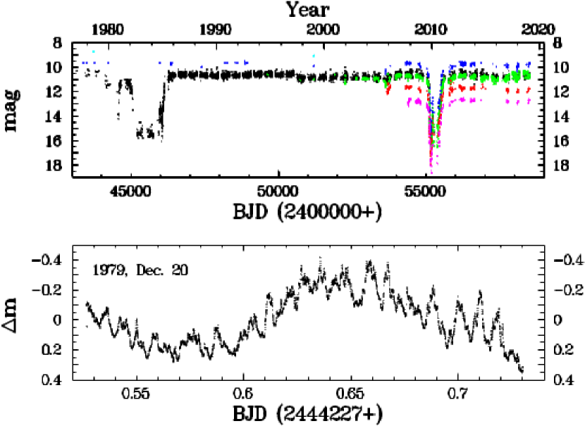
Figure 1: Top: The long term light curve of TT Ari binned in 1 d intervals. The black dots represent visual magnitudes. $U$, $B$, $V$, $R$ and $I$ measurements are shown in cyan, blue, green, red and magenta, respectively. For clarity, the $B$ and $U$ band data are shifted upwards by 1 mag and and $R$ and $I$ band data downwards by 1 and 2 mag, respectively. Bottom: Time resolved light curve of 1979 December 20 as a typical example, showing clear superhump variations together with flickering and QPOs.

Fig. 1 (top) contains the overall long term light curve. Visual magnitudes are shown as black dots. $I$, $R$, $V$, $B$ and (the few) $U$ data are colour coded in magenta, red, green, blue and cyan, respectively. For clarity, the $B$ and $U$ band data are shifted upwards by 1 mag, and the $R$ and $I$ band data downwards by 1 and 2 mag, respectively. All magnitudes have been binned in 1 day intervals. Since the data provided by E. Nather, I. Semeniuk, and E. Robinson are not calibrated, an average magnitude is assigned to them. As an example of the typical variations of TT Ari on the time-scale of hours, the lower frame of Fig. 1 shows the (unfiltered) light curve of 1979 December 20. The variations caused by the 3.2 h superhump are outstanding. Superposed is random flickering and (not clearly separated from flickering) a flaring activity with a limited regularity, identified as QPOs.

During most of the more than 40 yr of observations TT Ari remained in an almost stable (except for some small glitches) state of high brightness. However, as is well documented in the literature, during two time intervals it went into a deep low state, first for a prolonged period between the end of 1979 and the beginning of 1985, and then again for a shorter time between September 2009 and February 2011. The first of these was covered only by visual observations with a coarse time resolution. It is therefore not regarded here. The second low state, however, was extensively observed in $B$, $V$, $R$ and $I$, many times at a high time resolution. These observations reveal some interesting new features of TT Ari (see Sect. 4).

3 The high state

3.1 Superhumps

As mentioned in Sect. 1, TT Ari is well known to exhibit negative superhumps during most of the time it spends in the high state. Only during the brief interval between 1997 – 2004 they were replaced by positive superhumps. While they have been documented several times in the literature, the present data set permits a more rigorous assessment of its properties and evolution than has been possible in the past.

3.1.1 The extensive AAVSO data of 2012, 2014 and 2017

By far the most high state data, best suited for the purpose of this study, refer to the years after the second low state. Most of them consist of time resolved light curves, spanning up to several hours. For a timing analysis of the superhumps in these data I restrict myself to the $V$ band, and then only to the time resolved light curves having a resolution of better than 100 s and spanning at least 1 h. The most extensive data refer to the 2012 observing season, encompassing a total of 112 light curves (see Fig. 2, upper left frame). Most of the scatter in magnitude seen during individual nights is due to regular variations which can readily be identified as being caused by the superhump. Superposed, slight variations on longer time-scales are seen. These appear not to be random, indicating that differences in the calibration of individual light curves, which may be expected considering that the data were obtained by a variety of observers, remain small.

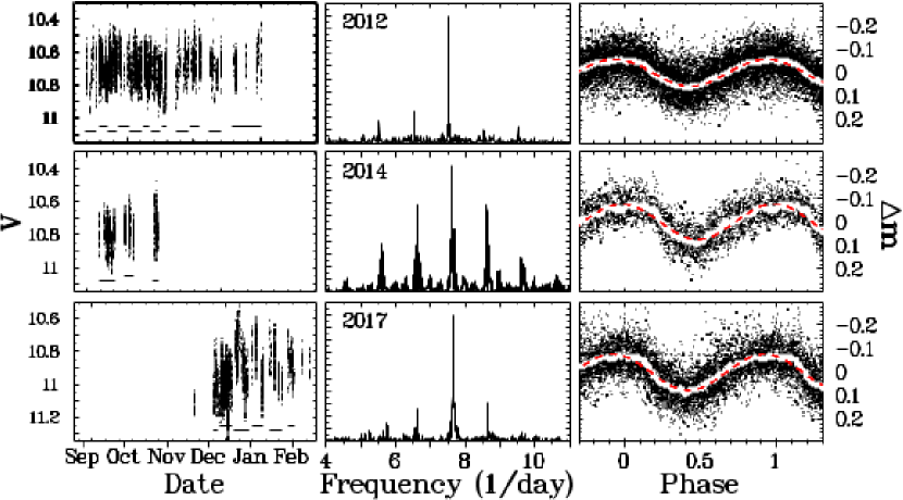
Figure 2: Left column: Combined $V$ band light curves observed during the 2012 (top), 2014 (middle) and 2017 (bottom) observing seasons. The bars beneath the light curves indicate the intervals used to search for possible variations of the superhump period (see text). Central column: Power spectra of the combined light curves. Right column: Light curves after subtraction of the night-to-night variations, folded on the period corresponding to the dominant peak in the power spectra. The white ribbons represent the same light curves, binned in phase intervals of width 0.01. The red broken graph is a least squares sine fit to the binned light curves.

In a first step the nightly mean was subtracted from the individual light curves. Then a Lomb-Scargle periodogram (Lomb, 1976; Scargle, 1982, hereafter also referred to as power spectrum) of the combined data set was calculated. A sharp peak dominating the spectrum provided the preliminary period of the superhump variations which are clearly seen in the individual light curves. In the next step a sine curve of the form $V=a\sin\left(2\pi(t-t_{o})/P\right)+\gamma$ was fit to each light curve. Here, $a$ is the half amplitude, $t$ the time of the observations, $t_{o}$ the zero point of phase, $P$ the period fixed to the preliminary value, and $\gamma$ is an offset in magnitude. This offset was then subtracted from each light curve. This procedure provides a better subtraction of night-to-night variations than simply subtracting the mean. The resulting combined data set was again submitted to the Lomb-Scargle algorithm, and the resulting power spectrum is shown in the upper central frame of Fig. 2.

The power spectrum is dominated by a strong peak, accompanied by secondary peaks at both sides which are 1 d^-1 aliases. The maximum provides the superhump period $P_{\rm SH}=0.1328743$ d, listed in the second column of Table 1 together with the error that (here and in all similar cases later) is propagated from the error in frequency, conservatively defined as the standard deviation of a Gaussian fit to the maximum in the power spectrum. The light curve, cleaned from night-to-night variations and folded on this period, is shown in the right upper frame of Fig. 2, where the maximum of the superhump waveform is taken to be the zero point of phase. The white ribbon in the folded light curve represents a binned version, using intervals of 0.01 in phase. The red broken line is a least squares sine fit, yielding a full amplitude $A_{\rm sh}$ of the modulation listed in the last but one column of Table 1.

Table 1: Properties of negative superhumps and related structure in the TT Ari light curves of observing seasons 2012, 2014 and 2017. Periods are expressed in days, amplitudes in magnitudes. The difference between $P_{\rm long}$ and $P_{\rm prec}$ is expressed in units of its statistical error.

year	$P_{\rm SH}$	$P_{\rm long}$	$P_{\rm prec}$	$P_{\rm long}-P_{\rm prec}$	$A_{\rm SH}$	$A_{\rm long}$
2012	0.132874	3.98	3.90858	–1.91	0.116	0.065
	$\pm$0.000037	$\pm$0.02	$\pm$0.03208		$\pm$0.003	$\pm$0.006
2014	0.132799	3.83	3.84456	–0.08	0.152	0.074
	$\pm$0.000139	$\pm$0.17	$\pm$0.11295		$\pm$0.011	$\pm$0.008
2017	0.132643	4.12	3.71806	3.50	0.154
	$\pm$0.000092	$\pm$0.09	$\pm$0.40344		$\pm$0.001

A close inspection of the folded light curve reveals that the superhump wave form is not quite sinusoidal. The decline from maximum is slightly steeper than the ascent. This asymmetry should be reflected in the power spectrum as signals at harmonic frequencies of the main peak. Indeed, it contains a weak maximum at $2f_{\rm SH}=15.052$ d^-1.

Next, the stability of the period was investigated. For this purpose, 12 sections of the whole 2012 light curve (marked by horizontal lines below the light curve in Fig. 2) were subjected to the Lomb-Scargle analysis. These sections are identified in Table 2 which also lists the superhump periods. The forth column contains the difference between the average period during the observing season and the period measured in the specific light curve section, expressed in units of the $1\sigma$ uncertainty of that difference. In only one section (BJD 2456227 – 2456230) no consistent periodic variations were obvious and in one other section (BJD 2456213 – 2456217) the peak frequency is significantly different from the average of the entire data set. All other subsections exhibit peak frequencies comfortably consistent within their error margins with the overall frequency. Therefore, there is no evidence for variations of the superhump period over the entire $\approx$4 month spanning the observations. The last column of the table contains the amplitudes of the modulations in the respective sections. They exhibit erratic variations which are significantly larger than their formal errors, these being of the order of 2 mmag.

Table 2: Periods (in days) and amplitudes (in magnitudes) of negative superhumps in restricted sections of the TT Ari light curves of observing seasons 2012, 2014 and 2017. The last but one column contains the difference between the period within a section and the average seasonal period, expressed in units of its statistical error.

Year	BJD	Period	Diff.	Amplitude
2012	2456169 – 177	0.132857	–0.03	0.156
	2456179 – 185	0.132700	–0.26	0.131
	2456185 – 192	0.132758	–0.19	0.131
	2456193 – 202	0.133184	0.46	0.110
	2456202 – 211	0.132431	–0.64	0.119
	2456213 – 217	0.133921	1.61	0.101
	2456219 – 226	0.133035	0.28	0.136
	2456227 – 230	–	–	0.00–
	2456236 – 246	0.132797	–0.14	0.085
	2456248 – 255	0.132691	–0.31	0.120
	2456262 – 271	0.132848	–0.04	0.122
	2456279 – 301	0.132800	–0.17	0.126
2014	2456909 – 921	0.132862	–0.02	0.160
	2456928 – 935	0.131581	–1.67	0.106
	2456949 – 953	0.132857	–0.01	0.195
2017	2458090 – 094	0.132380	–0.20	0.163
	2458095 – 105	0.132475	–0.41	0.173
	2458106 – 117	0.133037	0.22	0.140
	2458119 – 128	0.132505	–0.50	0.195
	2458132 – 142	0.132709	–0.23	0.174
	2458146 – 151	0.133145	0.21	0.149

In order to search for other periodic signals in the light curve, the best fitting sine curve with a period fixed to the superhump period was subtracted from each individual light curve and then the offset $\gamma$ of the fitted sine was added again. In this way the superhump variations are removed, but the combined light curve still contains variations on longer (and shorter) time scales. The corresponding power spectrum is shown in the upper left frame of Fig. 3. As listed in the third column of Table 1, the strongest peak corresponds to a period of $P_{\rm long}=3.9808$ d. On the other hand, the orbital period together with $P_{\rm SH}$ yield a beat period, interpreted as the precession period of the accretion disk, of $P_{\rm prec}=3.90857$ d (column 4 of Table 1). Thus, the difference $P_{\rm long}-P_{\rm prec}=-1.91\sigma$ (column 5 of Table 1), where $\sigma$ is the error of $P_{\rm long}-P_{\rm prec}$. Although $P_{\rm long}$ is not quite identical to $P_{\rm prec}$, considering the formal error limits, it appears that the precession of the accretion disk induces a slight variability in the brightness of the system, confirming earlier results of Semeniuk et al. (1987), Udalski (1988) and (1997). The light curve folded on $P_{\rm long}$ is shown in the upper right frame of Fig. 3. The white dots are a binned version of the folded light curves, using intervals of width 0.01 in phase. The red solid line is a least squares sine fit to the binned light curve. The amplitude is listed in the last column of Table 1.

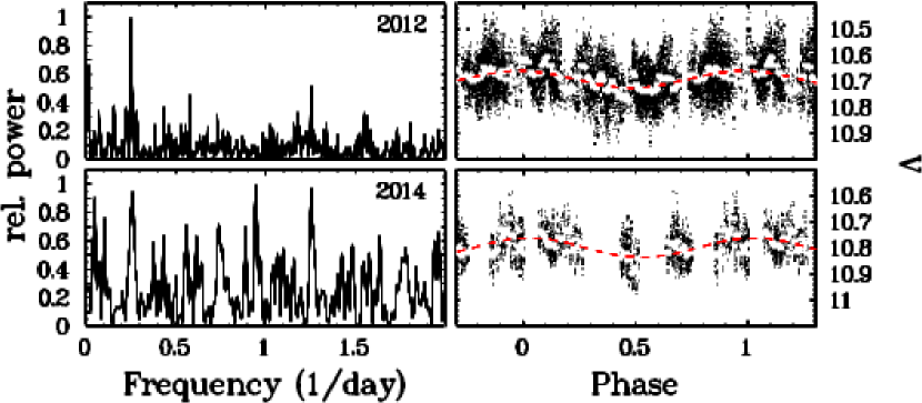
Figure 3: Left: Power spectra of the combined 2012 (top) and 2014 (bottom) light curves after removal of the superhump modulations. Right, combined lines curves, folded on the period corresponding to the power spectrum peak close to 0.25 d^-1. The white dots represent the same data, binned in phase intervals of width 0.01. The red curves are least squares sine fits to the binned light curves.

Similar exercises were performed for the 2014 and 2017 observing seasons, using 16 light curves observed between 2014 September 8 and October 22, and 48 light curve obtained between 2017 November 18 and 2018 February 12. The results are shown in Fig. 2 and listed in Tables 1 and 2. The superhump amplitude is similar in both seasons, but higher than observed in 2012. The waveform of the superhump deviates from a pure sine in the same way as in 2012. No significant period changes occur during the smaller observing intervals, but in 2017 the average period is slightly smaller than in previous seasons.

The power spectra of the residual light curves, after removing the superhump variation, do not reveal the beat frequency between orbit and superhump as clearly as in 2012. In 2014 (lower frames of Fig. 3) two peaks at different frequencies (not obviously related to other periodicities in the system) are about as strong as the maximum at 0.2612 d^-1 which I take to correspond to $P_{\rm long}$. However the close coincidence between $P_{\rm long}$ and $P_{\rm prec}$ and the amplitude of the corresponding variations which is quite similar to that measured in 2012 lend some confidence that a brightness modulation on the precession period really exists.

In 2017 this issue is less clear. The power spectrum of the residual light curve is rather inconclusive because the average magnitude of TT Ari varied much more during this season than in previous years (see Fig. 2). It is unclear whether these night-to-night variations are real or caused by uncertainties of the magnitude calibration of the light curves compiled from different sources. The power spectrum has only a minor peak close to the expected precession frequency. The corresponding period is quoted tentatively in Table 1 (in italics, in order to distinguish it from other, more reliable entries in the table), but the difference $P_{\rm long}-P_{\rm prec}$ being 3.5 times the error margin casts doubt on the presence of a modulation on the disk precession period. It is not sensible to quantify the amplitude of the light curve folded on that period in view of the much stronger night-to-night variations.

3.1.2 Re-analysis of the Kim et al. (2009) data

(2009) observed TT Ari in the $R$ band during 48 nights between 2005 October 27 and 2006 March 6. These data cover the recovery of the system from a minor downward glitch in its magnitude (see Fig. 1). TT Ari rose from an average magnitude of $R=11.25$ to a local brightness maximum of $R=10.3$ and then settled down at an intermediate level of about $R=10.7$ (see fig. 1 of , 2009). (2009) used times of minima in the light curves to measure the superhump period, but did not comment on the fact that superhumps were not present during the entire period of their observations.

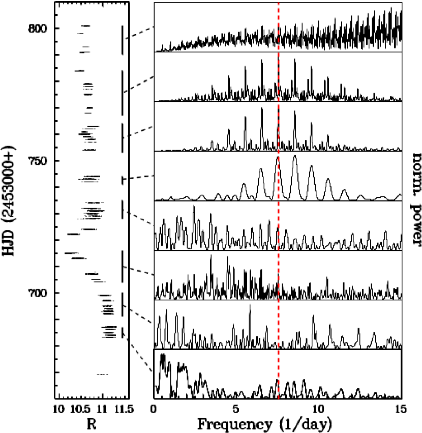
Figure 4: The combined light curves observed by (2009) (left) is shown together with power spectra (right) calculated from the light curve sections marked by vertical bars. The broken vertical line marks the frequency of the superhump modulation derived from the combined light curves in the interval HJD 2453741 – 84).

A re-analysis of their data, following the same procedures outlined in Sect. 3.1.1, reveals the evolution of superhumps over time. This is shown in Fig. 4. On the left hand side, the light curve is repeated. Vertical bars indicate intervals referring to the power spectra drawn on the right hand side of the diagram. These clearly show that a periodic signal at the superhump frequency (the broken vertical line, derived from the power spectrum of the combined data in the interval HJD 2453741 – 84) is at most marginally present during the faint state of TT Ari until just after the local maximum. Thereafter, the superhump evidently dominates the light curves. Somewhat surprisingly, during the end of the entire interval covered by (2009), it may still be present but is no longer outstanding. The development of the fully grown superhump occurs remarkably fast. Some trace may be present in the interval HJD 2453714 – 35, but only 6 d later (HJD 2453741) it is the dominant feature in the power spectrum. These time-scales should provide limits for models explaining their formation and destruction.

The superhump period of $0.132624\pm 0.000150$ d, derived from the light curve of the time interval when the superhump is clearly present, is slightly longer than that quoted by (2009) who used a different method for its determination. The amplitude is 0.094 mag. When comparing it to the amplitude observed at other epochs it should be remembered that it refers to $R$ band observations. As observed in most of the AAVSO data, the superhump waveform is slightly asymmetrical with a slower rise to maximum and a faster decline to minimum. No convincing evidence for a brightness modulation on the beat period between orbit and superhump was found.

3.1.3 Smaller data sets observed between 1977 and 2004

Smaller data sets are available for several other observing seasons. They are briefly discussed here. In most but not all cases the power spectra contain more or less clear evidence for superhumps. While the corresponding peaks are not always the strongest, but aliases, the closeness to the well established period seen at other epoch lends confidence in their reality. The resulting periods are summarized in Table 3 which also contains results compiled from the literature (see Sect. 3.1.4). It also lists the amplitude of the modulation as determined from a least squares sine fit, and the passband to which the amplitude refers. Depending on the distribution of the individual light curves within the observing window cycle counts are sometimes uncertain and thus the correct choice among the alias peaks in the periodogram is not always unique. Therefore, errors based on the width of the peaks will be misleading and are not quoted in the table. The left hand side of Fig. 5 shows the power spectra for each investigated season while the right hand side contains the phase folded light curves, binned in intervals of width 0.01 and a least square sine fit. The red (right) vertical line indicates the long-term average frequency of the negative superhump modulation (see Sect. 3.1.4), while the blue (left) vertical line is the positive superhump frequency as measured by Skillman et al. (1998).

In no case an assessment of the presence of variations on the beat period between superhump and orbit is possible due to the small number of nightly light curves and because many of them are nor calibrated and therefore lack a common magnitude scale.

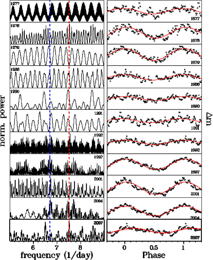
Figure 5: Left: Power spectra of fragmentary light curves observed in various years. The red (right) vertical line indicates the long-term average frequency of the negative superhump, while the blue (left) vertical line is the positive superhump frequency. Right: Light curves of the respective years, after subtraction of the nightly mean, folded on the period listed in Table 3 and binned in intervals of 0.01 in phase. The vertical scale of each diagram encompasses 0.3 mag, except for 1979 where it is twice this value. The red curves are least squares sine fits to the data.

1977: Three unfiltered (’white light’) light curves provided by E. Nather, observed between 1977 August 9 and December 15 yield a power spectrum with a peak (although not quite the highest) corresponding to a period of 0.134049 d, close to but still somewhat longer than the average superhump period.

1978: Two $U$ band and two $B$ band light curves observed between August 2 and 25 were kindly provided by I. Semeniuk. The $U$ band data are also listed by Schwarzenberg-Czerny et al. (1988). The power spectrum has a significant peak quite close to the expected superhump frequency. Folding the light curves on the respective periods indicates that the satellite peaks on both sides of the main one can be discarded as representing the true period. The folded light curve shown in Fig. 5 and the amplitude quoted in Table 3 only refer to the $U$ band where the superhump is more clearly expressed than in $B$.

1979: Only two light curves observed in white light, kindly provided by E. Nather, are available. However, obtained within four days on 1979 December 20 and 24, they are of extremely high quality and exhibit regular variations very clearly. Due to the insufficient time coverage the power spectrum of the combined light curves contains a forest of alias peaks which makes it impossible to select the “correct” one without pre-knowledge. The highest peak leads to a period of 0.150347 d, far from the expected negative superhump period, but remarkably close to the positive superhump period observed 2 yr later. However, there are no other reports indicating that the negative has been replaced by a positive superhump during this observing season. Only about two weeks earlier, Semeniuk et al. (1987) observed a negative superhump, albeit at a period somewhat higher than the average (see Sect. 3.1.4). The currently discussed light curve has a peak, only slightly lower than the highest one, which corresponds to $P=0.130953$ d, similar to the period identified by Semeniuk et al. (1987) and which is listed in Table 3. The amplitude of the modulations is at 0.33 mag much higher than observed at other epochs.

1985: Six $B$ band light curves provided by I. Semeniuk and S. Rössiger are available. However, although in some of the individual light curves systematic variations on time-scales roughly comparable to the expected superhump period are present, the overall light curve does not lead to a consistent picture. Therefore, these data are not considered further here.

1988: Three Walraven light curves observed between 1988 August 16 and 27 were kindly provided by A. Hollander. They have been discussed by Hollander & van Paradijs (1992). The power spectrum is dominated by a multitude of alias peaks. The maximum at 7.5152 d^-1, which I adopt here as the most relevant, is not the strongest one, but the corresponding period (0.13306 d) is very close to the expected negative superhump period. The closest and slightly stronger alias peak corresponds to 0.1299 d, much smaller than ever observed for the superhump. Moreover, the light curve folded on the adopted period supports the presence of consistent variations on this period. Its amplitude, listed in Table 3 refers to the $B$ band and was transformed from flux units as provided by the Walraven photometer (Walraven & Walraven, 1960; Rijf, Tinbergen & Walraven, 1969) into magnitudes.

1990: Six light curves observed in the Stiening system, kindly provided by E. Robinson are available. Five of them were observed between 1990 October 12 and 18. The last one is not considered here because of the long time difference of 64 d to the others which complicates the power spectrum significantly. The most prominent peaks in the power spectrum correspond to a period of 0.133831 d (rather far away from the superhump period observed in other years) and to its 1 d^-1 alias. The folded light curve, even after binning, is quite noisy and has a low amplitude, making it difficult to assess if the periodic modulation is spurious or real. Keeping this caveat in mind, the results are listed in Table 3

1991: The situation in 1991 is quite similar to that in the previous year. Again, six Stiening light curves are available, with 5 of them observed in the time window between 1991 October 4 and 12, and the last one in 1991 December. The latter is disregarded for the same reason as above. The power spectrum does not provide a clear picture. The highest peak corresponds to a period of 0.159425 d, far away from any expected superhump period. One of its aliases corresponds to 0.137334 d, more compatible but still significantly different from the superhump period in other seasons. Again, the folded light curve is of low amplitude and noisy, and is thus not quite convincing. Therefore, the same caveat expressed earlier must be kept in mind.

1992: Two data sets observed in 1992 are available. The first one consists of five $UBV$ light curves, kindly provided by T. Schimpke, observed between 1992 August 10 and 17. Four light curves in the Stiening system, provided by E. Robinson, obtained between September 24 and November 29 constitute the second set. The power spectrum is complex. However, the strongest peak corresponds to a period very close to the expected superhump period.

1997: By 1997, the negative superhump in TT Ari gave way to a positive superhump (Skillman et al., 1998). This is confirmed by five AAVSO light curves observed between 1997 December 1 and 1998 January 22. This time window is part of the larger window covered by Skillman et al. (1998). It is therefore not surprising that the dominant power spectrum peak yields a period of 0.14931 day, i.e., within the error limit of the period quoted by Skillman et al. (1998), based on more extensive data.

2001: The power spectrum of three light curves observed between 2001 December 4 and 24 has its strongest peak at a frequency corresponding to a period of 0.170048 d. However, there is an alias peak corresponding to 0.148441 d. While this is significantly different from the period observed in 1997, it is well known that in superoutburst of SU UMa type dwarf novae the (positive) superhump period is not stable but evolves over time (see, e.g., Kato et al., 2009). The same may be expected here. Moreover, between 2000 August and 2001 January, Stanishev, Kraicheva & Genkov (2001) observed a superhump period of 0.148815 d in the light curve as well as in the equivalent width of various emission lines. Therefore, the modulation in the present data seen at 0.148441 d may confidently be identified as the positive superhump in TT Ari. Its amplitude is similar to that observed in 1997.

2004: The power spectrum of six light curves observed between 2004 December 4 and 25 shows that the positive superhump still persists (see also Andronov et al., 2005). The amplitude appears to be slightly smaller than in previous years.

2007: Eight light curves are available for this season. They were observed in a comparatively small time window between 2007 October 23 and November 6. The superhump modulation is clearly present. The waveform deviates more strongly from a pure sine curve than in other seasons and in the opposite sense. It has a steeper rise to maximum and a more gradual decrease.

3.1.4 The long term properties of superhumps

The period of the negative superhumps has been measured many times at many different epochs. Therefore, its stability and systematic or stochastic variations can be assessed. In their table 3, Tremko et al. (1996) present a list of period determinations up to 1988. Since then, further measurements have become available which warrant an update, presented here in Table 3 together with the results of the present study. The table also includes (in italics) periods of the positive superhump observed between 1997 and 2004. A plot of the negative superhump period vs. time (not shown) does not suggest a systematic variation over more than half a century covered by data, but rather some small scale scatter. Averaged over the total time base the period is $0.13295\pm 0.00067$ days.

Table 3: Compilation of superhump periods and their amplitudes of TT Ari measured in different observing seasons since 1961

Year	Period	Amp.	Pass-	Reference
	(days)	(mag)	band
1961	0.1329			Smak & Stepien (1975)
1966	0.1327			Smak & Stepien (1975)
1977	0.1338			Semeniuk et al. (1987)
1977	0.13405	0.079	white	this work
1978	0.13280	0.176	$U$	this work
1978	0.1326	0.2	$B$	Sztajno (1979)
1979	0.13095	0.327	white	this work
1985	0.132771			Rößiger (1988)
1985	0.132765			Udalski (1988)
1985	0.1328			Semeniuk et al. (1987)
1986	0.13298			Volpi et al. (1988)
1987	0.132957			Udalski (1988)
1988	0.132816			(1992)
1988	0.132953			Tremko et al. (1992)
1988	0.13306	0.076	$B$	this work
1990	0.13383	0.059	$B$	this work
1991	0.13386	0.055	$B$	this work
1992	0.13215	0.061	$B$	this work
1994	0.133160	0.102	$B$	Andronov et al. (1999)
1994	0.1323	0.18a	$B$	Belova et al. (2013)
1995	0.1338	0.13b	$B$	Belova et al. (2013)
1995	0.13369	0.108	$B$	Kraicheva et al. (1999)
1996	0.13424	0.082	$B$	Kraicheva et al. (1999)
1997	0.14926	0.13c	$V$	Skillman et al. (1998)
1997	0.14931	0.150	$V$	this work
1997	0.14923	0.136	$B$	Kraicheva et al. (1999)
1998	0.14961	0.130	$B$	Kraicheva et al. (1999)
1999	0.14890			Wu et al. (2002)
2001	0.14844	0.169	$V$	this work
2001	0.1500	0.15d	$V$	Belova et al. (2013)
2004	0.14860	0.136	$V$	this work
2004	0.1483	0.20d	$R$	Belova et al. (2013)
2005	0.132322			(2009)
2005	0.132624	0.094	$V$	this work
2007	0.1324			Weingrill et al. (2009)
2007	0.13302	0.102	$V$	this work
2012	0.132874	0.116	$V$	this work
2014	0.132799	0.152	$V$	this work
2017	0.132643	0.154	$V$	this work
a estimated from fig. 3 of Belova et al. (2013)
b estimated from fig. 4 of Belova et al. (2013)
d estimated from fig. 1 of Skillman et al. (1998)
d estimated from fig. 2 of Belova et al. (2013)

The precession period of a tilted disk depends on the mass ratio of the stellar components, the tilt angle and the mass distribution in the disk. In the approximation of Larwood (1998) the latter resumes to the disk radius. Keeping the tilt angle and, of course, the mass ratio fixed, eq. (4) of Larwood (1998) shows that, in order to explain the observed scatter of the superhump period, changes of the disk radius of the order of 10 percent (or less, considering that a significant part of the scatter may be due to uncertainties to measure the period in small data sets) are required.

Whenever the corresponding information is available, the full amplitude of the modulation is also listed in table 3 together with the photometric band to which it refers. The negative superhump amplitude is quite variable with no clear systematic trends. Particularly striking is the huge amplitude observed in 1979. The 1992 data, consisting of five $UBV$ light curves and four light curves observed in the Stiening system, permit an assessment of the colours of the superhump. Neglecting the slight differences of the effective wavelengths of the passbands in the two systems, I find an average amplitude of $\Delta U=0.31$, $\Delta B=0.35$, $\Delta V=0.42$ and $\Delta R=0.53$. Thus, it increases to the red, suggesting that the modulation arises mainly in the outer, cooler parts of the accretion disk.

3.2 QPOs and flickering

Smak & Stepien (1969) were the first to draw attention to QPOs in TT Ari occurring on a time-scale of 14 – 20 min. They are readily visible in many light curves as flares with an amplitude of the order of 0.2 mag (see, e.g., the lower frame of Fig. 1), although they often cannot unequivocally be separated from random flickering.

Much effort has been invested in the past to characterize these QPOs and to find some regularity in their behaviour. While some authors content themselves to quote some favoured periods seen in their light curves (e.g., Williams, 1966; Udalski, 1988; Hollander & van Paradijs, 1992), others searched for systematic features in their long term behaviour (, 1997, 2009). Semeniuk et al. (1987) claim the detection of a systematic decrease of the QPO period from 27 m in 1961 to 17 m in 1985. This is contested by Tremko et al. (1996) who instead of a systematic trend suspect the presence of several preferred QPO frequencies. This view is also supported by Andronov et al. (1999) who find that the power spectra of their data contain significant peaks in the wide range between 24 and 139 d^-1 with the highest of them corresponding to periods of 21 and 30 m. Kraicheva et al. (1999) also found the QPOs to be highly unstable with a coherency limited to 3 – 8 cycles and power spectrum peaks detected in the 40 – 120 d^-1 range. From an autoregressive analysis they suggest that the QPOs are most probably generated by some stochastic process such as flickering. This blurs the border line between the two phenomena (see also Bruch, 2014).

3.2.1 QPO frequencies and their evolution

The wealth of the present data confirms the notion that not much regularity exists in the occurrence of the QPOs, except for a preference for a broad but limited frequency range. This is exemplified in Fig. 6 which contains the power spectra of a selection of light curves on different time-scales. For the left hand column, combined seasonal light curves of 5 different years were used, with intervals of roughly a decade between them (noting that the number of contributing individual light curves differs greatly). The central column contains the power spectra of the different time intervals in 2017, as defined in Table 2. Finally, the right hand column is based on the light curves of the individual nights of the last two time intervals. The coloured vertical lines, corresponding to periods of 15 (red, right), 20 (green, middle) and 30 (blue, left) minutes, are not meant to indicate specific features in the power spectra but have the sole purpose to guide the eye through the multitude of structures. The great variety of the power spectra in the figure indicates the chaotic frequency behaviour of the QPOs.

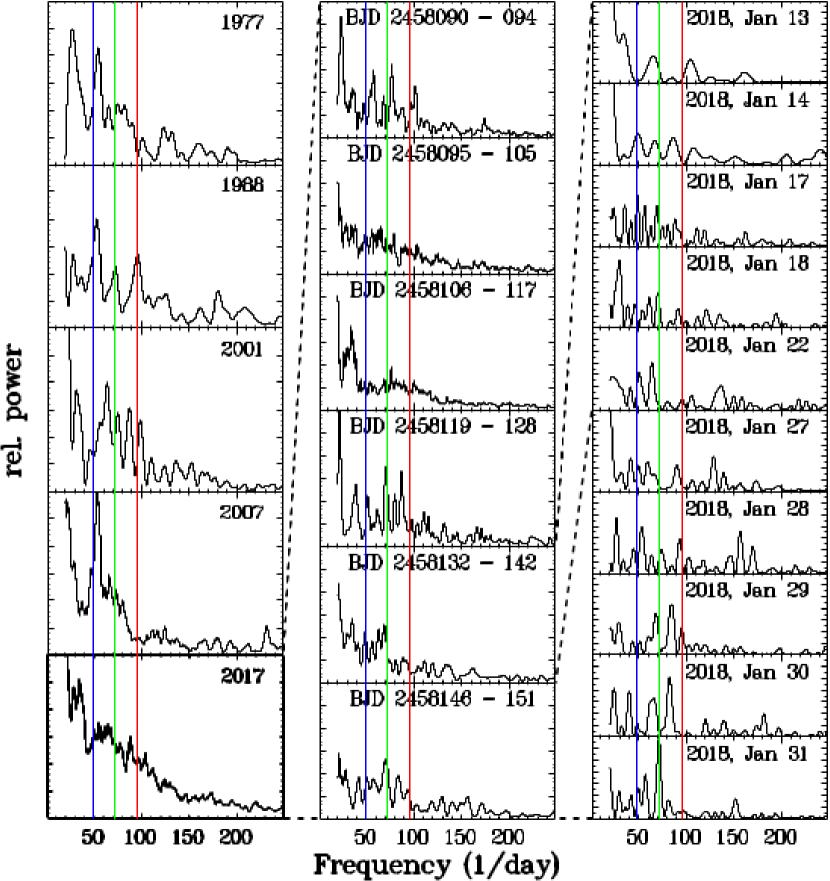
Figure 6: Examples of power spectra of light curves sampled on different time-scales: combined seasonal light curves (left), combined light curves of intervals encompassing several days (middle), and light curves of individual nights. The frequency range is restricted to the domain occupied by QPOs. The coloured vertical lines have the sole purpose to guide the eye and correspond to periods of 15 (red, right), 20 (green, middle) and 30 (blue, left) minutes.

The overall frequency range occupied by the QPOs can be assessed from the weighted average of the power spectra of all individual light curves, choosing a weight proportional to the total time base encompassed by the nightly data sets. The normalized sum of all power spectra, shown as a black graph in Fig. 7, has a dominant broad peak with its maximum corresponding to a period of 21.4 m and a total width corresponding to a period range between 18 and 25 m. Both, at lower and at higher frequencies, fainter peaks appear. Without trying to assess their formal significance, they indicate that QPOs appear to occur within some preferred period intervals between about 15 and 50 m, as claimed previously by Tremko et al. (1996) and Andronov et al. (1999).

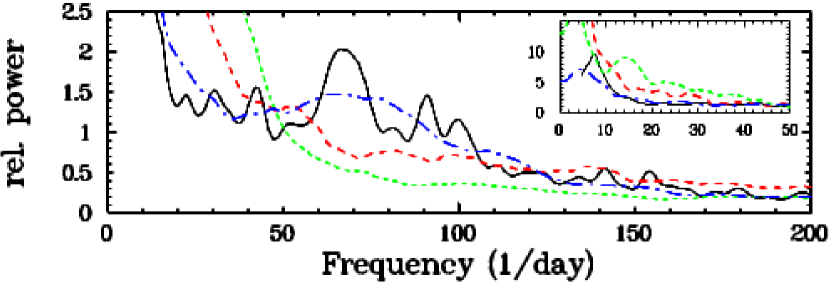
Figure 7: Normalized weighted average of the power spectra of individual light curves of TT Ari. The black graph refers the high state, the coloured ones to sections 1 (red, dashed), 2 (green, dotted) and 3 (blue, dashed-dotted) of the 2009 – 2011 low state (see text for details). The insert shows the low frequency part of the spectra on an expanded scale.

Assessing QPOs on the basis of power spectra of nightly light curves may be misleading. Stacked power spectra permit a more detailed view of their evolution over the time-scale of hours. For this purpose I selected some long and high quality data sets: two unfiltered light curves taken in 1977 by E. Nather and the $B$ band of two Stiening light curves observed in 1992 by E. Robinson. First, a filtered version, using a Savitzky-Golay filter (Savitzky & Golay, 1964), was subtracted from the original data, removing all modulations on time-scales above about 90 min (thus, the superhumps). Then, Lomb-Scargle periodograms for sections of a data train, 0.04 d long, were constructed, allowing for a strong overlap of 0.039 d between subsequent sections. Thus, each segment covers approximately 3 cycles of a typical QPO. The individual power spectra were then stacked on top of each other, resulting in a 2D representation (frequency vs. time) (for a more detailed description of this technique, see Bruch, 2014).

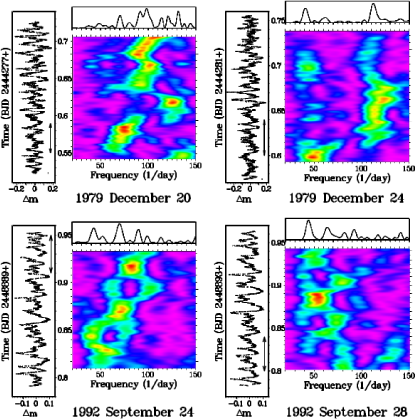
Figure 8: Stacked power spectra of TT Ari in four nights. The images show the power (colour coded) as a function of frequency (horizontal axis) and time (vertical axis). On the left, the light curves are shown after subtraction of variations on time-scales of more than 90 min. The double arrow indicates the length of the individual sections used to calculated the stacked power spectra. Thus vertical structures in the 2D images extending over less than the length of the arrow are not independent. On top of each stacked power spectrum the ’conventional’ periodogram of the entire data set it drawn.

The results are shown in Fig. 8 which, for each of the four nights, shows the high-pass filtered light curve in the left frames, the ’conventional’ power spectrum (using the entire light curve) on top, and the stacked power spectrum as a 2D colour coded image. The double arrow drawn beneath the light curves indicates the length of the individual data segments used to calculate the power spectra. Thus, any vertical structures in the images smaller than this length are not independent from each other.

The stacked power spectra suggest patterns in the occurrence of the QPOs. On 1977 December 20 (top left), and 1992 September 24 and 28 (bottom) there appears to be an evolution of the QPO frequency to higher or lower values over the time interval covered by the light curves. On 1977 December 20, this is interrupted by the short appearance of a signal at higher frequencies but is then resumed, while on 1992 September 24, the QPOs occasionally seem to split into two branches. On 1977 December 24 (top right), QPOs at two distinct frequencies are present, one getting fainter when the other grows stronger. The 1992 September 24 results are a good example of a misleading ’conventional’ power spectrum. It suggests the presence of three distinct frequencies, while the stacked version rather indicates an evolution of both, the frequency and the strength of the QPOs. Semeniuk et al. (1987) claim coherence of the QPOs over intervals of at least 6 h (and possibly even from night to night). While the present data, in most cases, cannot confirm coherence, they show that the same train of events may persist over several hours, gradually changing frequency.

3.2.2 Flickering and QPO amplitudes

The definition of the amplitude (or strength) of the ubiquitous flickering in the light curves of cataclysmic variables is not trivial and, to my knowledge, has never been done rigorously and objectively. The standard deviation, variance or rms-scatter of individual magnitude measurements in a light curve is occasionally taken to be a measure of the flickering strength (e.g., Dobrzycka, Kenyon & Milone, 1996; Dobrotka, Mineshige & Ness, 2015). This is certainly to be preferred to simply adopting the magnitude difference between the peaks of flickering flares and the troughs between them, since the latter depends more strongly on individual and random features in a light curve, while the former take into account their average. Even so, there are some pitfalls which a more rigorous approach has to consider.

Postponing a more detailed description to an upcoming paper (Bruch, in preparation) I hereafter briefly summarize the method used to quantify the strength of the flickering in CVs. Most importantly, variations unrelated to flickering have to be removed. If these have longer time-scales (e.g., orbital modulations or superhumps) this is easily done by subtracting a filtered version of the original data. I use a Savitzky-Golay filter with a cut-off time-scale of 60 minutes. In the case of TT Ari this does not separate the QPOs from flickering (if such a separation is meaningful at all; see the brief discussion in Bruch, 2014). Thus, here I will study the combined strength of QPOs and flickering which is in most light curve dominated by the QPOs. Variations on short time scales, distinct from flickering (such as dwarf nova oscillation, see Warner, 2004) are only resolved in high time resolution light curves and generally of low amplitude. They can therefore be neglected. A histogram is constructed from the individual magnitude data in the high-pass filtered light curve. As is shown in the left frame of Fig. 9, it can in general well be approximated by a Gaussian. I take the full width at half maximum (FWHM) as a proxy of the flickering strength and denote it as $A_{60}$, considering that it only contemplates variations on time-scales smaller than 60 min. Note that $A_{60}$ is smaller than but proportional to the average amplitude of flickering flares. It enables the comparison of the flickering strength in different light curves and in different systems.

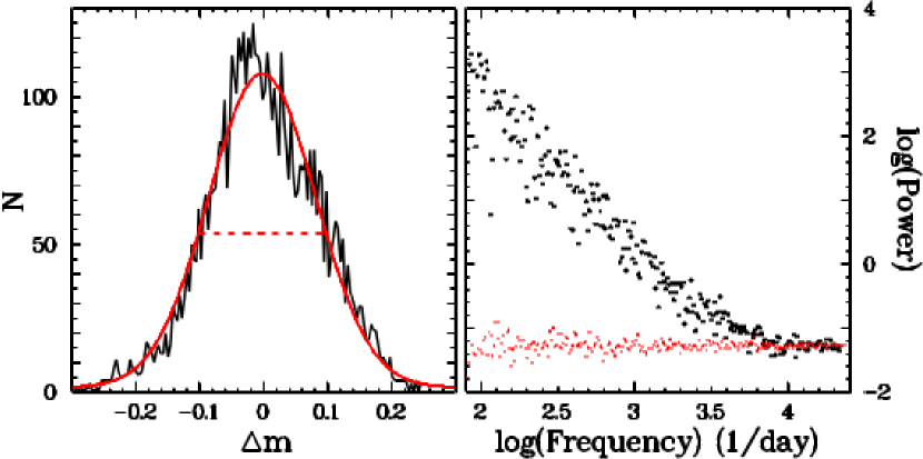
Figure 9: Left: Illustration for the measurement of the flickering strength: Histogram of the distribution of data points in a flickering light curve (black) and best fit Gauss curve (solid red). Its FWHM (broken red line) is defined as the flickering amplitude. Right: Illustration for the determination of the noise level in a flickering light curve: Black dots are a log-log representation of its power spectrum. The smaller red dots represent the average power spectra of 10 light curves of pure Gaussian noise, sampled in the same way as the real light curve, with the noise amplitude adjusted to the flat high frequency part of the power spectrum of the real light curve.

$A_{60}$ is a measure similar to the variance of data points in a light curve. However, some corrections are required. The most obvious one is a correction for noise in the data which widens the distribution of data points. If the noise can be regarded as Gaussian, the variance of the observed data is simply the sum of the variance due to noise and to real variations. A correction is then easy. The problem obviously lies in the determination of the noise level in the data. Here, the well known red noise characteristic of flickering helps. As shown in the right frame of Fig. 9, the power spectrum of a flickering light curve (larger black dots), drawn on a double-logarithmic scale, slopes downward linearly at high frequencies, but levels off to a constant at very high frequencies, where it is dominated by white noise. Generating a power spectrum of pure Gaussian noise (smaller red dots in the figure), sampled in the same way as the real light curve, with an amplitude such that it matches the flat part of the flickering light curve power spectrum, provides the noise level in the data.

Another correction concerns the time resolution of the data. Larger integration times act as a filter reducing the height and depth of extrema. Thus, a reduction of $A_{60}$ to a reference time resolution, which I define to be 5 s, is required. This effect depends on the time-scale on which flickering events predominantly occur, which may differ from one object to the other. It can be accounted for, determining a correction factor as a function of the time resolution. For this purpose, a high quality light curve observed with the reference (or higher) time resolution is binned into intervals, simulating a reduced resolution. Comparing $A_{60}$ measured at the reference and at other time-scales provides the correction factor.

A third correction, required in some cases, can be omitted here. It concerns the contribution of the secondary star light that dilutes the flickering. However, in TT Ari in the high state it is wholly negligible.

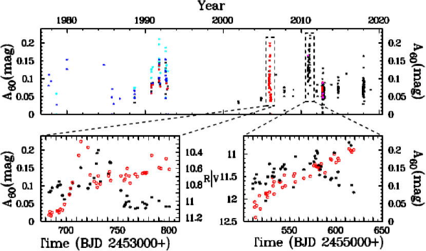
Figure 10: Top: Flickering amplitude $A_{60}$ as a function of time for observations taken in $U$ (cyan), $B$ or white light (blue), $V$ black, $R$ (red) and $I$ (magenta). Bottom: Amplified view of two limited time intervals in 2005 and 2010 – 2011 marked in the upper frame. In addition to $A_{60}$ (black dots) the mean nightly magnitudes are shown as red circles.

$A_{60}$ was measured in all high state light curves of TT Ari and is shown as a function of time in the upper frame of Fig. 10. The colours reflect the observed passbands: $U$ (cyan), $B$ or white light (blue), $V$ (black), $R$ (red) and $I$ (magenta). $A_{60}$ scatters significantly. This is partly due to measurement errors caused mainly by two effects: (i) in light curves with a comparatively small number of data points the histogram of their distribution is not well defined, leading to uncertainties of the FWHM of the fitted Gaussian; and (ii) in light curves with a coarse time resolution the Nyquist frequency is such that the useful part of the power spectrum does not reach the plateau at high frequencies, enabling only to determine an upper limit to the noise level. However, these effects cannot mask real and systematic variations of the flickering amplitude which are particularly evident in two sections of the long term light curve.

These sections are shown in more detail in the lower frames of Fig. 10. Here, the red circles indicate the average magnitude of the respective light curves. Both sections correspond to periods when TT Ari underwent particular phases in its long term behaviour. The left frame refers to the data of (2009). As was mentioned in Sect. 3.1.2, TT Ari recovered from a minor excursion to fainter magnitudes. $A_{60}$ assumed an intermediate level when the system was still at the bottom of this excursion, goes through the maximum and then settles at a lower level when TT Ari assumed its long-term high state magnitude after a short term maximum. It is interesting to note that the maximum of $A_{60}$ is assumed only about two weeks after the maximum in brightness. Thus, there is no strict correlation between flickering amplitude and system magnitude. This is also seen in the second section (right lower frame of Fig. 10) which corresponds to the very end of the recovery of TT Ari from the low state in 2009 – 2011. Here, $A_{60}$ rises from an intermediate level, goes through a maximum, and then declines to the same level as before, while the brightness of the system rises steadily during the entire time interval.

Concluding this section, I briefly investigate the wavelength dependence of the flickering amplitude. For this purpose I restrict myself to the simultaneous multicolour observations provided by A. Hollander (Walraven system), T. Schimpke (Johnson $UBV$) and E. Robinson (Stiening $UBVR$ system) in order not to mix data of different passbands obtained at different epochs. The slight differences of the effective wavelengths of the passbands in the three photometric systems are neglected, adopting the effective wavelengths of the $UBVRI$ system as tabulated by Bessell (2005). The average value of $A_{60}$ in the $UBVR$ passbands is shown as a function of wavelength in Fig. 11 which reflects the well known flickering property in CVs to increase in strength to the blue and UV. The error bars are mean errors of the mean which are a better representation for the accuracy of the average value than the standard deviation. It must be noted, however, that the figure does not reflect directly the spectral energy distribution (SED) of the flickering light source. This would only be true if the constant (i.e., not flickering) components of the system (basically the quiet light of the accretion disk), upon which flickering is superposed, had the same SED. This is not necessarily the case.

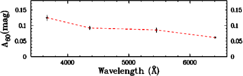
Figure 11: Wavelength dependence of the flickering amplitude in TT Ari.

4 The 2009 – 2011 low state

In contrast to the high state, the two deep low states observed in TT Ari in 1979 — 1985 and 2009 – 2011 have received much less attention. The first one was treated in some detail by Shafter et al. (1985) and later by Gänsicke et al. (1999), while Hutchings & Cote (1985) presented some complementary observations. To my knowledge, the only paper discussing observations of the 2009 – 2011 low state was published by Melikian et al. (2010). Apart from some time resolved light curves observed by Shafter et al. (1985) not much detailed photometry performed in this state has been studied. In particular, the AAVSO data of the first low state consist only of isolated visual observations which are of little use for the investigation of variations on short time-scales. This is different when it comes to the second low state, parts of which have extensively been covered with high time resolution light curves obtained by AAVSO observers.

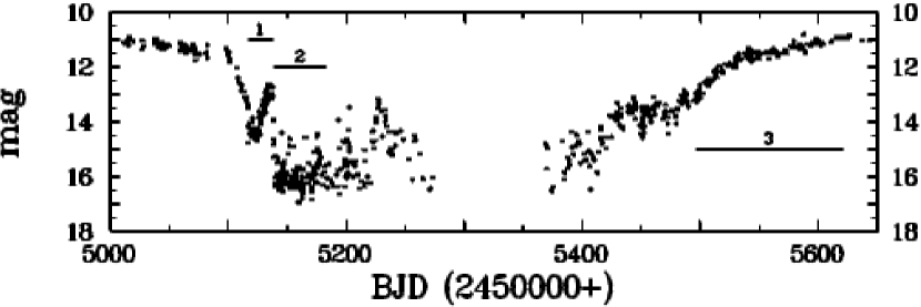
Figure 12: Light curve of TT Ari during its 2009 – 2011 low state, binned into 1 day intervals. The horizontal lines indicate 3 sections discussed in more detail in the text.

An expanded view of the long-term light curve during the 2009 – 2011 low state is shown in Fig. 12, where the data have been binned in 1 day intervals. In view of the strong variations in comparison to the colour indices of TT Ari, for visualization purposes measurements in different passbands are not distinguished in the figure. The overall evolution is such that an initial drop by 3.3 mag, lasting 26 d, is followed by a $\approx$8 d plateau and a subsequent steady rise by 1.7 mag over $\approx$12 d. This is reminiscent of the start of the 1979 – 1985 low state (Fig. 1) when TT Ari also recovered almost to the high state magnitude after an initial drop, albeit on longer time scales. This first recovery is followd by a precipitously drop by 3.3 mag to $\approx$16.3 mag within less than 3 d. After a plateau lasting about 80 d (much of the scatter in this phase is caused by the specific sampling of strong intra-night variations; see below) a rapid brightness increase to another local maximum and a subsequent drop to the same low level is observed. Following the seasonal gap in the observations, TT Ari starts a continuous recovery from the low state, exhibiting four phases with distinct gradients in the light curve.

Three sections of the low state light curve are of particular interests. These are marked by horizontal lines in Fig. 12, and will subsequently be discussed in more detail.

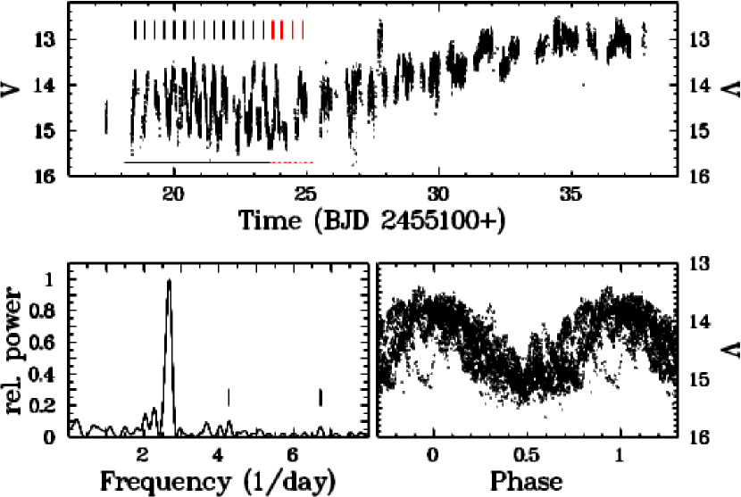
Figure 13: $V$ band light curve of the plateau phase and the subsequent rise after the initial drop of TT Ari into the low state (upper frame). The horizontal line below the light curve indicates a section with strong oscillations which are coherent at first (black) but later loose coherence (dotted red). The vertical tick marks are the predicted times of maxima calculated using the period corresponding to the peak frequency of the power spectrum (lower left frame; the two marked features are discussed in the text) based on the part of the light which exhibits coherent modulations. The lower right frame contains the light curve folded on the period.

4.1 Coherent large amplitude modulations

The first section refers to the short lived plateau and subsequent rise after the initial plunge from the high state. The upper frame of Fig. 13 presents an expanded view of this section, maintaining the original time resolution. Apparently periodic large amplitude variations are immediately evident during the plateau phase. It turns out that they lose coherence towards the end. Therefore two intervals of the plateau phase were defined, distinguished by the black and dotted red horizontal lines below the light curve. The power spectrum of the first of these intervals is shown in the left lower frame of Fig. 13. The outstanding peak corresponds to a period of $0.372\pm 0.011$ d. The vertical bars in the upper frame of the figure, spaced with this period, indicate the excellent alignment with the light curve maxima in the first interval, which is lost during the latter part of the plateau phase. The lower right frame shows the coherent part of the light curve, folded on the period. The total amplitude of the variations amounts to $\approx$1.2 mag.

The power spectrum contains many minor peaks that, however, are all statistically significant. For most of them no simple relation between their frequencies is evident. It is worthwhile, however, to draw attention to a small peak (but still with a maximum power more than 10 times stronger than the 0.0001 false alarm probability level as calculated using the prescription of Bruch, 2016) close to 6.7 d^-1 (marked with a vertical bar in the figure), corresponding to a period of $0.1487\pm 0.0014$ d. Coincidence or not, this is very close to the centre of the period range of the positive superhumps observed in 1997 – 2004. Moreover, curiously, this period and the main period of 0.372 d, within less than 1 percent of their formal errors, are multiples (2$\times$ and 5$\times$, respectively) of a basic period of 0.0744 days. They may therefore be regarded as overtones of each other. Another peak (also marked in the figure) corresponds to a period of $0.233\pm 0.003$ d, close to (but beyond the formal error limit) three times this basic period. I leave it open if the relationship of these periods with the positive superhump period has any physical meaning, or if I am over interpreting the data.

After the plateau phase a steady increase of the brightness sets in. While intra night variation on the level of some tenths of a magnitude still occur, no evidence of any regularity from night to night could be detected. Flickering is present during the entire section discussed here.

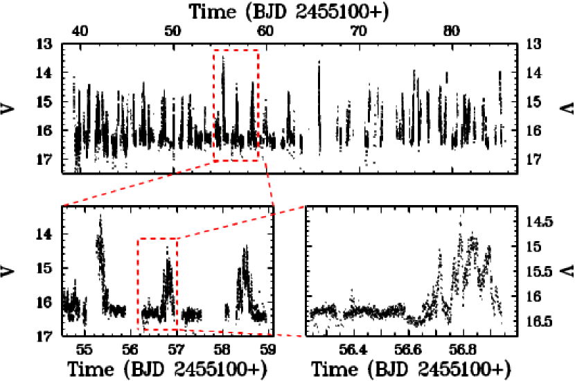
Figure 14: Light curve during the deep low state of TT Ari together with views with increasing time resolution of a light curve section.

4.2 The deep low state

The second section refers to the bottom of the low state (hereafter: the deep low state) after the second rapid drop in brightness. The upper frame of Fig. 14 contains the light curve of the entire section, while a small part of it is shown in increasing detail in the lower frames. Disregarding some excursions to even lower magnitudes (which may well be due to measurement uncertainties at this quite low brightness level for the instruments used by many AAVSO observers) the light curve shows a quite well defined lower limit of about 16.3 mag.

Using observations taken during the 1979 – 1985 low state, Gänsicke et al. (1999) estimate the visual magnitude of the secondary star to be 19.07 mag and the temperature of the white dwarf as 39 000 K. The latter is a close match to EC 11437-3124 which, at a temperature of 38 810 K (Gianninas, Bergeron & Ruiz, 2011), has $V=17.32$. At 208.6 pc (Bailer-Jones et al., 2018) its distance is slightly less than that of TT Ari. Correcting for this difference it should have $V=17.53$ at the distance of TT Ari. This is an upper limit for the brightness of the TT Ari white dwarf because Gianninas, Bergeron & Ruiz (2011) estimate a mass of $0.69\ M_{\odot}$ for EC 11437-3124, less than the (uncertain) mass of TT Ari that should thus have a smaller radius and be less luminous. The combined light of the stellar components of TT Ari should therefore not be brighter than $V=17.3$, a magnitude fainter than the observed lower limit in the light curve. This implies (an) additional light source(s) in the system, which may be a residual accretion disk.

4.2.1 Intermittent activity

The lower brightness limit of 16.3 mag is defined by quiet phases with are interrupted by strong flares with amplitudes typically of $\approx$1.5 mag but that can reach almost 3 mag. There is no strict periodicity in the occurrence of the latter, but the median interval of 1 d between them is quite well defined, and they last for about 5 – 8 h. As is best seen in the lower right frame of Fig. 14, individual flares are heavily structured. Melikian et al. (2010) have already drawn attention to this flaring activity of TT Ari during the low state. However, their limited amount of data did not permit a more thorough characterization of this behaviour.

The quiet phases are seen only during a limited time interval, covering most of the minimum between the first and the second re-brightening during the low state. The sampling of the light curve becomes less dense during the second half of the section shown in Fig. 14, but it appears that the number and duration of the quiet phases decreases. At later times (not show in detail), the sampling becomes even less complete which makes any statement about the occurrence of quiet phases less secure. However the last time resolved light curve without significant variability was observed on 2009 December 25, i.e., before the second re-brightening. All subsequent observations contain strong irregular variations on the time-scale of hours.

The lack of observations makes it difficult to assess if the alternation of quiet phases and strong flaring activity also occurred during the first deep low state of TT Ari. The AAVSO long term light curve, restricted to visual magnitude estimates, does not have sufficient time resolution to answer this question. But it contains some points which lie about 1 mag above the mean low state level, suggesting flares. Moreover, the limited time resolved observations discussed by Shafter et al. (1985) includes light curves at a similar brightness level as the present quiet phases with only low-scale flickering over time intervals of $\approx$3 h. Thus, the overall behaviour may have been similar during the 1979 – 1985 low state.

The alternation between quiet and flaring phases during the low state of VY Scl stars is not unheard of. While in most such systems the available low state observations are not sufficient to explore this question, the long uninterrupted high cadence observations of MV Lyr by the Kepler satellite enabled (2017) to detect a similar behaviour in that star. The variations seen in the bottom frame of their fig. 1 bear much resemblance with the TT Ari deep low state behaviour, although some differences are also obvious. Even not being strictly periodic, the flares occur much more regularly in MV Lyr. The burst duration and typical intervals are 30 m and 2 h, respectively, versus 5 – 8 h and 1 d in TT Ari. These numbers make the duty cycle of the flares quite similar in both systems. The flare amplitudes are also similar, being typically $\approx$1.5 mag and occasionally even larger.

(2017) explain the flaring behaviour of MV Lyr within a magnetic gating model, where a magnetic field of the primary star disrupts the inner disk out to the co-rotation radius, forming a centrifugal barrier. Matter in the disk then accumulates outside the barrier, increasing the pressure until it is overcome, permitting accretion onto the white dwarf and releasing bursts in the process. (2017) show that, depending mainly on the mass accretion rate and the white dwarf spin period, a magnetic field as low as 22 kG, too small to be directly detectable, may be sufficient to create the barrier. Once the accretion rate rises above a certain limit and thus the system becomes brighter, the magnetic field is no more able to create the barrier and the intermittent flaring behaviour stops.

A similar model may be able to explain the deep low state behaviour of TT Ari. Not knowing important system parameters, in particular the rotation period of the white dwarf which determines the co-rotation radius, it is difficult to assess if the model is compatible with the details of the observations along the lines investigated for MV Lyr by (2017). An argument in favour of the presence of a weak magnetic field is the finding of Thomas & Wood (2015) in their SHP simulations that a field in the kilogauss regime can lead to the emergence of negative superhumps in novalike systems. On the other hand, if matter accumulates outside the centrifugal barrier between flares, a gradual increase of the system brightness during the non-flaring phases may be expected but is not seen. This is equivalent to the lack of brightening, contrary to theoretical predictions, of dwarf novae between outbursts (Lasota, 2001).

A further drawback of the magnetic gating model is the fact that, while explaining the alternation between quiet and flaring phases during the deep low state, another explanation is required for the continuous strong and either a-periodic or periodic (see Sect. 4.1) variations seen at higher brightness levels throughout the low state. Assuming as a single mechanism modulations of residual mass transfer from the secondary star may be able to account for both. The involved time-scales of hours are easily compatible with dynamical (free fall) time-scales in the binary system.

While it is a broadly accepted view that the low states in VY Scl stars (as well as those observed in some members of the magnetic subclass of CVs) are caused by a decrease or cessation of mass transfer from the secondary components, the reason for this decrease are less clear. The most thoroughly discussed scenario, first elaborated by Livio & Pringle (1994), is that of star spots crossing the L₁ region. The cooler gas in the spots has a smaller scale height than the undisturbed stellar atmosphere. It can therefore detach from the L₁ point, reducing or inhibiting mass transfer. Elaborating this scenario further and applying it to the low state of AM Her, Hessman, Gänsicke & Mattei (2000) assume not a single spot but a heavily structure star spot region to be responsible for strong variations of the mass transfer rate in AM Her and consequently of the brighness during this state. A similar situation may explain the low state variations occurring over the course of weeks in TT Ari. The strong modulations on the time-scale of hours may then be due to hydromagnetic exchange instabilities, as already speculated by Livio & Pringle (1994). This leaves open only the reason for the strict periodicity seen in the first part of section 1.

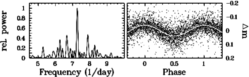
Figure 15: Left: Power spectrum of non-flaring phases of the light curve of TT Ari during the deep low state. The dominant peak occurs at the orbital frequency. Right: Low state light curve folded on the orbital period. The white line is a least squares sine fit.

4.2.2 Orbital variations

During the quiet phases the brightness of TT Ari is not quite constant. In spite of the significant noise at this low light level, some light curves clearly exhibit variability. It is different, however, from the flickering activity observed by Shafter et al. (1985) at a similar magnitude and noise level. While flickering may still be present in the data discussed here, but may be more difficult to detect above the noise because of a much lower time resolution than that of the Shafter et al. (1985) data, more obvious are consistent variations on the time-scale of hours. I selected eight light curves in the time interval between 2009 November 17 and 25, where these modulations are best seen. After subtracting night-to-night variations they were subjected to the Lomb-Scargle algorithm. The resulting power spectrum is shown in the left frame of Fig. 15 and is dominated by a strong peak at 7.270 d^-1. The secondary peaks are either 1 d^-1 aliases or can be explained as being caused by the window function.

The peak frequency corresponds exactly to the spectroscopic orbital period of TT Ari. Thus, for the first time, a clear photometric manifestation of the binary revolution is observed. The light curve, folded on the orbital period, is shown in the right frame of Fig. 15. A formal sine fit (white curve) yields a total amplitude of 0.078 mag for the modulation. The epoch of the maximum is BJD 2455152.716. The spectroscopically determined epoch of the inferior conjunction of the primary component, closest to the epoch of the present observations, cited in table 3 of Wu et al. (2002), together with their orbital period, yields a phase difference of $0.06\pm 0.03$ between conjunction and light curve maximum. Here, the error includes only the formal period uncertainty. The true error may be larger. Thus, the modulations are consistent with an illumination of the secondary star by the white dwarf, this extra light being best visible to the observer at the inferior conjunction of the latter.

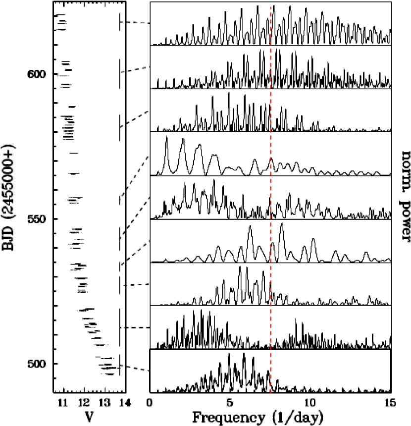
Figure 16: Light curve during the rise from the low to the high state (left) together with power spectra (right) calculated from the light curve sections marked by vertical bars. The red vertical line indicates the average frequency of the superhump modulation, derived from Table 3.

4.3 The rise towards the high state

The third section refers to the rise from the low to the high state. The entire rise phase, starting even before section 3, can clearly be separated into four parts: a gradual rise followed by a plateau; thereafter a steeper rise with a gradient of $0.034\,{\rm mag\,d{{}^{-1}}}$ sets in, before TT Ari approaches the high state at a much slower pace of $0.009\,{\rm mag\,d{{}^{-1}}}$.

The steep part and then the much flatter final rise are reminiscent of the observations of Honeycutt & Kafka (2004) who found distinct gradients during the start and/or the end of low states in several other VY Scl stars, with the steeper slope always occurring when the system was fainter. Within the star spot scenario for the low states Honeycutt & Kafka (2004) interpret the different gradients as being caused by the passage of the umbra (steeper slope) and penumbra (flatter slope) underneath the L₁ point. A similar situation may be realized in TT Ari. However, the behaviour at the onset of the rise points at a more complex situation (see also Sect. 4.2.1).

Section 3 was also selected because it is of interest in order to investigate if and, in case, when and at which brightness level TT Ari develops the superhumps seen at later epochs. For this purpose, the light curves were subjected to the same analysis which has been applied to the Kim et al. (2009) data in Sect. 3.1.2. The results are shown in Fig. 16 which is organized in the same way as Fig. 4. No consistent picture emerges. At most, the power spectra contain some indications that modulations on the time-scales of hours repeat over a few nights. In particular, although in some of the spectra a peak aligns approximately with the red vertical line which indicates the average superhump frequency calculated from Table 3, these may well be chance alignments.

4.4 Stochastic variations during the low state

Except for the strong 0.372 d oscillations observed during the first part of section 1 and the slight orbital modulations during the quiet phases of the deep low state, no regularly repeating variations could be detected during the low state. However, the average power spectra of the individual light curves within the three sections defined in Fig. 12, calculated in the same way as has been done for the high state light curves (Sect. 3.2.1), exhibit systematic differences. They are shown in Fig. 7 as red (dashed), green (dotted)0 and blue (dashed-dotted) lines for sections 1, 2 and 3, respectively. During section 2 only the flaring parts of the light curves were considered. Since due to the smaller number of individual light curves the average power spectra are rather noisy they have been smoothed in frequency by a bock filter of half-width 6 d^-1. The insert in the figure contains the low frequency part of the power spectra (unsmoothed) on an expanded vertical scale.

The average power spectrum of section 1 (red) exhibits, after a steep decline from a strong maximum at low frequencies (a reflection of the 0.372 d oscillations), a steady decline towards higher frequencies. On a double logarithmic scale it is strictly linear, as is the case for flickering activity in CVs in general. During section 2 (green), when quiet intervals alternate with strong flares, the high frequency part also shows a behaviour typical of flickering, but there is a pronounced peak (see insert in Fig. 7) centred on 13.4 d^-1 ($\approx$1.8 h), reflecting the time-scale of the main structures within flares. In both, section 1 and 2, no indication for the occurrence of QPOs as observed during the high state is seen. Finally, during section 3 (blue), while TT Ari recovers from the low state, the average power spectrum contains a distinct hump between 40 and 90 d^-1 which apparently indicates the re-appearance of QPOs. It is already present in the steeper part of the recovery from the low state, but becomes stronger during the final rise.

5 Conclusions

Complementing previous studies, I have investigated variations in the novalike variable TT Arietis with an emphasis on time-scale of hours and smaller, using an unprecedented wealth of data obtained over more then 40 yr during high and low states. During most of the time interval covered by the observations, the system remained in its normal high state, suffering only slight variations around its average magnitude. The main findings during this stage are:

1. The well known negative superhump, being replaced by a positive superhump only during the limited time interval between 1997 and 2004, persists to the present day. While within a given observing season its period was found to be stable, small variations occur from year to year. The long term average period is $0.13295\pm 0.00067$ d (3.1908 h). The full amplitude is quite variable, ranging from a staggering 0.33 mag in 1979 to low values of about 0.06 mag in several other years. Confirming earlier reports based on smaller data sets, in the two observing seasons, when the quantity and quality of the present observations permit a respective statement, a modulation on the precession period of the inclined accretion disk is also seen.

2. In observations taken during the 2005 observing season, when TT Ari recovered from a short lived excursion to a fainter magnitude and went through a local maximum before settling down to the average high state brightness, the superhump was initially absent but then rapidly emerged on the time-scale of only a few days.

3. QPOs are present during the entire high state. They occur preferentially in the quasi-period range between 18 and 25 m. In some light curves the evolution of their frequency and amplitude could be followed for several hours. In most of them a systematic evolution towards higher or lower frequencies is seen, while in one night two distinct frequencies appear to alternate.

Of the two deep low states suffered by TT Ari, that of 2009 – 2011 was very well covered by observations, permitting for the first time a detailed characterization:

1. The overall low state light curve is strongly structured on the time scale of tens of days. The rise to the high state occurs in four stages with distinct gradients.

2. After the first plunge into the low state, but still a magnitude above the deep low state attained later, during about five days TT Ari undergoes coherent large scale oscillations with an amplitude of $\approx$1.2 mag and a period of 8.93 h.

3. During the deep minimum at 16.3 mag TT Ari alternates on time-scales of roughly one day between quiet phases and strong (1.5 – 3 mag) flares. These last for 5 – 8 h and are highly structured on a preferred time-scale of 1.8 h. During the quiet phases the brightness is modulated on the orbital period. The phasing of these variations is consistent with reflection of radiation of the hot primary off the secondary star.

4. Strong variations on the time-scale of hours are seen throughout the low state, except during the quiet phase at its deepest parts. They are irregular but for the short coherent period at the beginning of the low state mentioned earlier. No clear signal of a superhump is seen even during the final rise to the high state. However, the $\approx$20 m QPOs first re-emerge during the steep part of the rise and grow stronger as the system approaches the high state.

References

- (1) Andronov I. L., Kolosov D. E., Movchan A. I., Rudenko A. N., 1992, SoSAO, 69, 79
- Andronov et al. (1999) Andronov I. L., et al., 1999, AJ, 117, 574
- Andronov et al. (2005) Andronov I. L., et al., 2005, IBVS, 5664, 1
- Bailer-Jones et al. (2018) Bailer-Jones C. A. L., Rybizki J., Fouesneau M., Mantelet G., Andrae R., 2018, AJ, 156, 58
- Belova et al. (2013) Belova A. I., et al., 2013, AstL, 39, 111
- Bessell (2005) Bessell M. S., 2005, ARA&A, 43, 293
- Bruch (2014) Bruch A., 2014, A&A, 566, A101
- Bruch (2016) Bruch A., 2016, NewA, 46, 60
- Bruch & Cook (2018) Bruch A., Cook L. M., 2018, NewA, 63, 1
- (10) Cowley A. P., Crampton D., Hutchings J. B., Marlborough J. M., 1975, ApJ, 195, 413
- Deeming (1975) Deeming T. J., 1975, Ap&SS, 36, 137
- Dobrotka, Mineshige & Ness (2015) Dobrotka A., Mineshige S., Ness J.-U., 2015, MNRAS, 447, 3162
- Dobrzycka, Kenyon & Milone (1996) Dobrzycka D., Kenyon S. J., Milone A. A. E., 1996, AJ, 111, 414
- Eastman, Siverd & Gaudi (2010) Eastman J., Siverd R., Gaudi B. S., 2010, PASP, 122, 935
- Gänsicke et al. (1999) Gänsicke B. T., Sion E. M., Beuermann K., Fabian D., Cheng F. H., Krautter J., 1999, A&A, 347, 178
- Gianninas, Bergeron & Ruiz (2011) Gianninas A., Bergeron P., Ruiz M. T., 2011, ApJ, 743, 138
- Hessman, Gänsicke & Mattei (2000) Hessman F. V., Gänsicke B. T., Mattei J. A., 2000, A&A, 361, 952
- Hirose & Osaki (1990) Hirose M., Osaki Y., 1990, PASJ, 42, 135
- Hollander & van Paradijs (1992) Hollander A., van Paradijs J., 1992, A&A, 265, 77
- Honeycutt & Kafka (2004) Honeycutt R. K., Kafka S., 2004, AJ, 128, 1279
- Horne & Stiening (1985) Horne K., Stiening R. F., 1985, MNRAS, 216, 933
- Hutchings & Cote (1985) Hutchings J. B., Cote T. J., 1985, PASP, 97, 847
- Kato et al. (2009) Kato T., et al., 2009, PASJ, 61, S395
- (24) Kim Y., Andronov I. L., Cha S. M., Chinarova L. L., Yoon J. N., 2009, A&A, 496, 765
- Kozhevnikov (2007) Kozhevnikov V. P., 2007, MNRAS, 378, 955
- Kozhevnikov (2012) Kozhevnikov V. P., 2012, NewA, 17, 38
- (27) Kraicheva Z., Stanishev V., Iliev L., Antov A., Genkov V., 1997, A&AS, 122, 123
- Kraicheva et al. (1999) Kraicheva Z., Stanishev V., Genkov V., Iliev L., 1999, A&A, 351, 607
- Larwood (1998) Larwood J., 1998, MNRAS, 299, L32
- Lasota (2001) Lasota J.-P., 2001, NewAR, 45, 449
- Livio & Pringle (1994) Livio M., Pringle J. E., 1994, ApJ, 427, 956
- Lomb (1976) Lomb N. R., 1976, Ap&SS, 39, 447
- Melikian et al. (2010) Melikian N. D., Tamazian V. S., Docobo J. A., Karapetian A. A., Kostandian G. R., Henden A. A., 2010, Ap, 53, 373
- Papadaki et al. (2006) Papadaki C., et al., 2006, A&A, 456, 599
- Papadaki et al. (2009) Papadaki C., Boffin H. M. J., Stanishev V., Boumis P., Akras S., Sterken C., 2009, JAD, 15, 1
- Patterson & Skillman (1994) Patterson J., Skillman D. R., 1994, PASP, 106, 1141
- Patterson et al. (2001) Patterson J., Thorstensen J. R., Fried R., Skillman D. R., Cook L. M., Jensen L., 2001, PASP, 113, 72
- Patterson et al. (2005) Patterson J., et al., 2005, PASP, 117, 1204
- Rette, et al. (2003) Retter A., et al., 2003, MNRAS, 340, 679
- Rijf, Tinbergen & Walraven (1969) Rijf R., Tinbergen J., Walraven T., 1969, BAN, 20, 279
- Rößiger (1987) Rößiger S., 1987, IBVS, 3007, 1
- Rößiger (1988) Rößiger S., 1988, MitVS, 11, 112
- Savitzky & Golay (1964) Savitzky A., Golay M. J. E., 1964, AnaCh, 36, 1627
- Scargle (1982) Scargle J. D., 1982, ApJ, 263, 835
- (45) Scaringi S., Maccarone T. J., D’Angelo C., Knigge C., Groot P. J., 2017, Nature, 552, 210
- Schwarzenberg-Czerny et al. (1988) Schwarzenberg-Czerny A., Semeniuk I., Tremko J., Urban Z., Zboril M., 1988, CoSka, 17, 49
- Semeniuk et al. (1987) Semeniuk I., Schwarzenberg-Czerny A., Duerbeck H., Hoffmann M., Smak J., Stepien K., Tremko J., 1987, Ap&SS, 130, 167
- Shafter et al. (1985) Shafter A. W., Szkody P., Liebert J., Penning W. R., Bond H. E., Grauer A. D., 1985, ApJ, 290, 707
- Skillman et al. (1998) Skillman D. R., et al., 1998, ApJL, 503, L67
- Smak & Stepien (1969) Smak J., Stepien K., 1969, CoKon, 65, 355
- Smak & Stepien (1975) Smak J., Stepien K., 1975, AcA, 25, 379
- Stanishev, Kraicheva & Genkov (2001) Stanishev V., Kraicheva Z., Genkov V., 2001, A&A, 379, 185
- Strohmeier, Kippenhahn & Geyer (1957) Strohmeier W., Kippenhahn R., Geyer E., 1957, Veröff. Remeis Sternw. Bamberg, 18
- Sztajno (1979) Sztajno M., 1979, IBVS, 1710, 1
- Thomas & Wood (2015) Thomas D. M., Wood M. A., 2015, ApJ, 803, 55
- Thorstensen, Smak & Hessman (1985) Thorstensen J. R., Smak J., Hessman F. V., 1985, PASP, 97, 437
- Tremko et al. (1992) Tremko J., Andronov I. L., Luthardt R., Pajdosz G., Patkos L., Rößiger S., Zola S., 1992, IBVS, 3763, 1
- Tremko et al. (1996) Tremko J., et al., 1996, A&A, 312, 121
- Udalski (1988) Udalski A., 1988, AcA, 38, 315
- Volpi et al. (1988) Volpi A., Natali G., D’Antona F., 1988, A&A, 193, 87
- Walraven & Walraven (1960) Walraven T., Walraven J. H., 1960, BAN, 15, 67
- Warner (1995) Warner B., 1995, CAS, 28
- Warner (2004) Warner B., 2004, PASP, 116, 115
- Weingrill et al. (2009) Weingrill J., et al., 2009, CoAst, 159, 114
- Whitehurst (1988) Whitehurst R., 1988, MNRAS, 232, 35
- Whitehurst & King (1991) Whitehurst R., King A., 1991, MNRAS, 249, 25
- Williams (1966) Williams J. O., 1966, PASP, 78, 279
- Wood & Burke (2007) Wood M. A., Burke C. J., 2007, ApJ, 661, 1042
- Wu et al. (2002) Wu X., Li Z., Ding Y., Zhang Z., Li Z., 2002, ApJ, 569, 418