pForest: In-Network Inference with Random Forests

Abstract.

When classifying network traffic, a key challenge is deciding when to perform the classification, i.e., after how many packets. Too early, and the decision basis is too thin to classify a flow confidently; too late, and the tardy labeling delays crucial actions (e.g., shutting down an attack) and invests computational resources for too long (e.g., tracking and storing features). Moreover, the optimal decision timing varies across flows.

We present pForest, a system for “As Soon As Possible” (ASAP) in-network classification according to supervised machine learning models on top of programmable data planes. pForest automatically classifies each flow as soon as its label is sufficiently established, not sooner, not later. A key challenge behind pForest is finding a strategy for dynamically adapting the features and the classification logic during the lifetime of a flow. pForest solves this problem by: (i) training random forest models tailored to different phases of a flow; and (ii) dynamically switching between these models in real time, on a per-packet basis. pForest models are tuned to fit the constraints of programmable switches (e.g., no floating points, no loops, and limited memory) while providing a high accuracy.

We implemented a prototype of pForest in Python (training) and P4 (inference). Our evaluation shows that pForest can classify traffic ASAP for hundreds of thousands of flows, with a classification score that is on-par with software-based solutions.

1. Introduction

Classifying network traffic in real time is an online classification problem which consists in predicting label(s) from a possibly unbounded stream of packets. Examples of classification tasks abound in networking and include: detecting attacks (e.g., DDoS) (Doshi et al., 2018), distinguishing mice flows from elephant flows (Zhang et al., 2021), identifying encrypted video streams (Schuster and Tromer, 2017), predicting flow length (Ðukic et al., 2019), website fingerprinting (Hayes and Danezis, 2016), device fingerprinting (Formby et al., 2016; Meidan et al., 2017), and many more.

A key challenge in online classification is deciding when to perform the classification, i.e., after how many packets. When done too early, the decision basis is too thin to classify a flow confidently. When done too late, the tardy labeling delays crucial actions. For instance, in the context of attacks, late classification might translate to service disruption (e.g., in the context of Pulse-Wave attacks (Seals, 2017)). Moreover, late classification wastes computational resources (e.g., tracking and storing features for unnecessarily long). Notably, the optimal decision timing varies across flows.

In an ideal world, network traffic flows would be classified whenever the label is sufficiently established – “As Soon As Possible”

(ASAP) – never sooner, never later. What makes ASAP classification hard, though, is that the optimal number of packets to consider for a classification task heavily depends on the traffic workload, the task itself, and even the individual flow. In short, a one-size-fits-all solution does not work. Nowadays, in-network classifiers do not support ASAP classification (we discuss related work at length in §10). Existing solutions either classify packets at the end of the flow (Lee and Singh, 2020), or classify all flows at the same packet count (Hullar et al., 2011; Bernaille et al., 2006b; Gómez Sena and Belzarena, 2009; Bernaille et al., 2006a), ignoring whether classification is possible on a per-flow basis. As our evaluation shows, both approaches are suboptimal in practice.

pForest  In this paper, we describe pForest, a system which enables programmable data planes to perform real-time, ASAP inference, accurately and at scale, according to supervised machine learning (ML) models. pForest takes as input a labeled dataset (e.g., an annotated traffic trace) and automatically trains a P4${}_{\text{}}$-based (Bosshart et al., 2014) online classifier that can run directly in the data plane and accurately infer labels on live traffic. Despite being performed in the data plane and as-soon-as-can-be, pForest’s inference is accurate. In fact, we show that it is as accurate as an offline, software-based classification using state-of-the-art ML frameworks such as scikit-learn (sci, 2022).

Challenges  Performing accurate ASAP inference in the data plane is challenging for at least three reasons. First, both the set and values of the relevant features change over a flow’s lifetime. As an example, the average packet length may be important to classify young flows, but for older flows, the total packet length may be more relevant. The values of the latter feature diverge as the flow progresses, so the optimal classification rules may change as well. ASAP inference therefore requires to dynamically adapt the selected features and ML models over the lifetime of a flow. pForest addresses this problem by training a sequence of random forests—dubbed “context-dependent random forests”—that maps to the different phases of a flow. The data plane applies this sequence during the life of a flow until the candidate label is certain enough; pForest decides on a per-flow basis when the soonest classification is possible.

Second, programmable switches are heavily limited in terms of the operations they support. In particular, they lack the ability to perform floating point computations which makes it hard to implement inference procedures for most ML models (e.g., neural networks) or to keep track of statistical features (e.g., the average or standard deviation). pForest addresses this problem by: (i) classifying traffic according to Random Forest ($RF$) models whose decision procedures (based on sequential comparisons) fit well within the pipeline of programmable switches; and (ii) automatically approximating statistical features. While pForest is restricted to $RFs$, we stress that $RFs$ are amongst the most powerful and successful ML models currently available (they can even emulate neural networks (Frosst and Hinton, 2017)) and tend to work well in practice (Biau et al., 2019; Arzani et al., 2020, 2016). Recent works have also successfully managed to apply $RFs$ to traffic classification tasks (e.g., (Ðukic et al., 2019; Hayes and Danezis, 2016; Arzani et al., 2020, 2016)), yet without supporting ASAP inference. Finally, $RFs$ are easily interpretable.

Third, programmable switches have a limited amount of memory (few tens of megabytes (Jin et al., 2017)) and do not support dynamic memory management. Yet, pForest needs to compute and store an unknown amount of features during inference in addition to storing the $RFs$. pForest addresses this problem by considering data-plane constraints while training the $RFs$ and selecting features that require small amounts of memory. A key insight is that this optimization does not come at the price of classification score. To further deal with the lack of dynamic memory, pForest relies on encoding techniques to pack multiple features in the same register.

We implemented pForest in P4₁₆ (data-plane inference) and in Python (training pipeline): given some hardware parameters, pForest automatically synthesizes all P4 code and dynamic CLI input necessary for inference in the data plane. Our implementation also supports dynamic model reloading.

Our evaluation shows that pForest can perform ASAP traffic classification at line rate, for hundreds of thousands of flows, and with an classification score that is on-par with software-based solutions. We further confirm that all the basic operations required by pForest are supported on existing hardware devices (Intel Tofino).

Note that pForest is a general framework that enables ASAP in-network inference. As such, it does not remove the need to obtain a representative training dataset. As for any ML model, poor input data will result in poor performance. We consider the problem of building a representative dataset as orthogonal to this paper.

Contributions  To sum up, our main contributions are:

• An optimization technique for computing random forest models and optimal feature sets tailored to perform as-soon-as-possible classification on programmable data planes (§4);

• A compilation technique for compiling random forest models to programmable network devices (§5);

• An allocation technique for dynamic memory management available for feature storage (§6);

• A prototype implementation in Python and P4${}_{\text{}}$, with a confirmation that pForest’s basic operations run on existing hardware (§7);

• An extensive evaluation using synthetic and real datasets (§8).

2. Background

In this section, we summarize the key concepts of programmable data planes (§2.1); we explain the gist of random forest classifiers (§2.2); and we define the notation (§2.3).

2.1. Programmable data planes

We implemented the data plane component of pForest in P4${}_{\text{}}$ (Bosshart et al., 2014), a programming language for network data planes. A P4${}_{\text{}}$ program consists of three main building blocks: a parser, which extracts header data from packets arriving at an ingress port; a match&action pipeline, which implements the program’s control logic with simple instructions and by applying match&action tables; and a deparser, which assembles and sends the final packet to an egress port. We describe key components and limitations of P4${}_{\text{}}$ below.

Tables  Match&action tables map keys (e.g., packet headers) to actions (e.g., set egress port). Adding and removing entries to tables is only possible via the control plane API.

Registers  Registers are stateful objects that are write- and readable both from the control plane and the data plane. They are organized as arrays of a fixed length and consist of entries with a fixed width. The size of registers needs to be declared at compilation time. Since there are no public specifications for the amount of memory in existing hardware devices, we report the results for units of 10MB.

Operations  P4${}_{\text{}}$ supports basic operations but no floating point computations or loops. pForest requires the following operations, all of which are supported by P4${}_{\text{16}}$ (P41, 2018) and bmv2 (Consortium, 2020): add, subtract, max, min, bit shift, bit slice.

Hardware architecture and resources  Programmable network devices implement the PISA architecture (Daly and Cascaval, 2017), which contains a fixed number of stages during which match&action tables are applied. The number of these stages limits the maximum number of tables that can be applied in sequence.

$$\begin{array}[]{lrcl}\lx@intercol\textbf{Flows}\hfil\lx@intercol\\[1.99997pt] \textit{(Flow)}&F&=&(\text{src IP},\text{dst IP},\\ &&&\;\;\text{src port},\text{dst port},\text{prot.})\\ \textit{(Packet)}&F[i]&&i^{\text{ th}}\text{ packet of the flow}\\ \textit{(Subflow)}&F[i:j]&&[F[i],F[i+1],\ldots,F[j-1]]\\ \textit{(Set of flows)}&\mathcal{F}&=&\{F_{1},F_{2},F_{3},\ldots\}\\ \textit{(Set of subflows)}&\mathcal{F}[i:j]&=&\{F_{1}[i:j],F_{2}[i:j],\ldots\}\\ &&&\\ \lx@intercol\textbf{Features}\hfil\lx@intercol\\[1.99997pt] \lx@intercol\textit{(Features of }\mathcal{F}\text{)}\hfil\lx@intercol&\operatorname{A}(\mathcal{F}),\quad\operatorname{A}\in\mathbb{R}^{m\times n}\\ &&&\\ \lx@intercol\textbf{Models}\hfil\lx@intercol\\[1.99997pt] \lx@intercol\textit{(Random forest)}\hfil\lx@intercol&RF\\ \lx@intercol\textit{(RF trained on }\operatorname{A}(\mathcal{F}[:i])\text{)}\hfil\lx@intercol&RF_{i}\\ \lx@intercol\textit{(RF applied to }F\text{)}\hfil\lx@intercol&RF(F)\\ \lx@intercol\textit{(Classifier)}\hfil\lx@intercol&\operatorname{C}&=&\{RF_{a},RF_{b},RF_{c},\ldots\},\\ &&&\{a,b,c,\ldots\}\subset\mathbb{N}\\ \lx@intercol\textit{(Decision tree)}\hfil\lx@intercol&DT\\ &&&\\ \lx@intercol\textbf{Metrics}\hfil\lx@intercol\\[1.99997pt] \lx@intercol\textit{(\{True,Predicted\} label)}\hfil\lx@intercol&\text{label}(F),\text{label}(RF(F))\\ \lx@intercol\textit{(Certainty)}\hfil\lx@intercol&\text{certainty}(RF(F))\\ \lx@intercol\textit{($F_{1}$ score)}\hfil\lx@intercol&\operatorname{F_{1}}(RF(\mathcal{F}))\\ &&&\\ \lx@intercol\textbf{Thresholds}\hfil\lx@intercol\\[1.99997pt] \textit{(Score threshold)}&\tau_{s}&\in&[0,1]\\ \textit{(Certainty threshold)}&\tau_{c}&\in&[0,1]\\ \end{array}$$

Figure 1. pForest notation and metrics

2.2. Random forest classifiers

A random forest ($RF$) (Ho, 1995) is a supervised ML classifier which consists of an ensemble of decision trees ($DTs$). To classify a sample, it applies all $DTs$ on the sample’s feature values, obtaining a label (i.e., estimated class) from each tree. Majority voting results in the final label. Additionally, each $DT$ can return a certainty score $\frac{x_{l}}{x_{tot}}$ where $x_{tot}$ is the number of training samples that ended up in the respective leaf node and $x_{l}$ is the size of the subset of them with the same label as the current sample. The $RF$’s certainty for this sample is the mean value of the individual certainties.

2.3. Notation

We depict our notation and definitions in Fig. 1. We identify a flow $F$ as a sequence of packets ($F[i]$ for $i\in[0,1,\ldots,|F|-1]$) sharing the same 5-tuple (source IP, destination IP, source port, destination port, protocol). A subflow is denoted as $F[i:j]$ and consequently the first $n$ packets of a flow are denoted by $F[0:n]$ or simply $F[:n]$. Sets of flows (as in the datasets that we use to train the classifier) are denoted as $\mathcal{F}$, sets of subflows as $\mathcal{F}[i:j]$.

Random forest models are abbreviated by $RF$, and a model that is trained with $\mathcal{F}[:n]$ is denoted as $RF_{n}$. $\text{label}(RF(F))$ denotes the label that $RF$ predicts for $F$, $\text{certainty}(RF(F))$ the certainty of the prediction, and $\operatorname{F_{1}}(RF)$ the F₁ macro-score of the model.

In training and inference, we use two thresholds: $\tau_{s}$ to denote the minimum F₁ score that is required to accept a model, and $\tau_{c}$ to denote the minimum certainty required to accept a label.

3. pForest overview

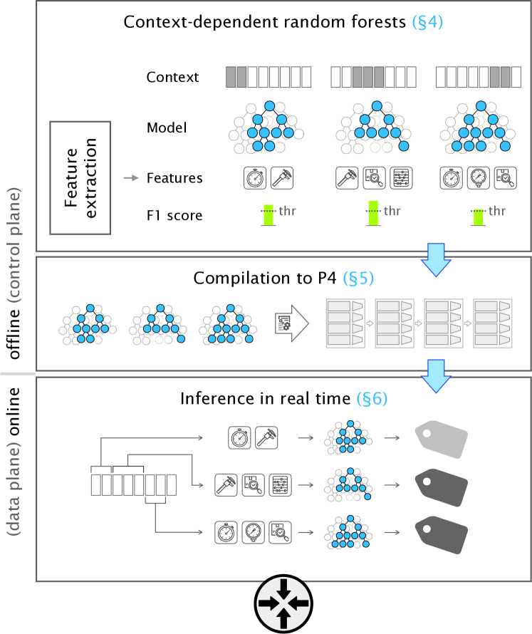
Figure 2. pForest overview. From a labeled training dataset, pForest extracts features and computes context-dependent $\boldsymbol{RFs}$. Afterwards, it compiles these models to program code and configurations for programmable network devices. These programmable network devices then apply the models in real time to network traffic.

In this section, we describe how pForest performs ASAP inference with $RF$ models entirely in the data plane of a network.

By ASAP inference, we refer to the concept of classifiying a flow as soon as a “confident” classification is possible. In the following, we go into more detail on (i) soon classification and on (ii) the notion of confidence behind possible classification, and then (iii) put both pieces together into as-soon-as-possible inference.

Soon classification  Observing an additional packet for a given flow can either improve the classification confidence or keep it at the same level, since strictly more information is given. Naturally, the most certain decision is possible after a flow has ended. Therefore, there exists a trade-off between classification confidence and classification speed. pForest allows for explicitly selecting a point in this trade-off via a threshold on the minimal confidence. With this threshold, it can decide on a per-flow level whether it has already observed enough packets to make a sufficiently confident decision, or whether it should wait for additional packets. However, this threshold on confidence is only conceptual. In reality, we cannot directly access a single confidence metric, but rather measure this concept as described in the next paragraph.

Possible classification  In order to assess the confidence for a flow’s candidate label, pForest uses a combination of two thresholds: First, a given $RF$ can report how certain it is about a label for a given sample. pForest can therefore only accept labels whose certainty exceeds a given threshold $\tau_{c}$. Second, if the $RF$ itself has a low quality, it may return a high certainty for wrong labels. Thus, pForest also applies a threshold $\tau_{s}$ to the $RF$ score.

ASAP inference  Putting the insights on soon and possible classification together, we arrive at ASAP inference. Concretely, it has two ingredients, namely context-dependent $RFs$ and certainty-based labeling. First, as established, the classification speed may vary across flows. Therefore, pForest needs to train a sequence of high-quality $RFs$ that can classify flows at various stages (context-dependent $RFs$). Recall that “high-quality” refers to exceeding $\tau_{s}$. This is the offline component of ASAP inference. Second, at runtime, pForest applies the $RF$ sequence throughout a flow’s progress. Each $RF$ reports a candidate label and how certain it is about this label. As soon as the certainty exceeds $\tau_{c}$, pForest accepts the label and stops the classification process (certainty-based labeling). This is the online component of ASAP inference.

Overall, this results in the following workflow, also depicted in Fig. 2: Initially, pForest takes a labeled training dataset and extracts features which are feasible to compute in programmable network devices. Based on these features, pForest computes context-dependent $RF$s which exceed a required minimum score, while minimizing the required hardware memory. Afterwards, pForest compiles the $RFs$ to data-plane programs. Note that we can perform all these operations offline in the control plane. Finally, pForest deploys the compiled models in programmable network devices which use them to perform runtime inference on the observed network traffic.

Feature extraction from the training data  pForest uses supervised ML and therefore requires a labeled dataset to train the $RFs$ which can support an arbitrary number of labels (i.e., traffic classes). Since the models match subflows of different lengths ($F[:n]$ for length $n\in\mathbb{N}$), the training dataset contains network traffic at packet level (e.g., in PCAP format without payload information).

pForest can use up to 18 popular network traffic features per subflow (i.e., $F[:n]$ for subflow length $n$) and it computes them in a way that is feasible in programmable network devices (e.g., replacing averages by moving averages).

Context-dependent RFs  During training, pForest trains multiple $RF$s for different contexts, i.e., different numbers of packets that have arrived for a flow. The goal is to maximize the score of each $RF$ while minimizing their required resources. As these objectives are opposed, pForest requires the operator to provide a score threshold $\tau_{s}$, turning one objective into a constraint. A high $\tau_{s}$ indicates that performance is more important than resource optimization (and vice-versa). pForest then reduces the resources allocated to a single $RF$ until any further reduction would drop its score below $\tau_{s}$.

pForest employs several methods to reduce the required resources, e.g., memory space. As an example, the same $RF$ is shared between multiple contexts if its score exceeds $\tau_{s}$ for all of them. Additionally, pForest removes redundant features and reuses them over different contexts to minimize the required feature memory.

Compiling RFs to data plane programs  After training context-dependent $RFs$ in software, pForest compiles them for use in programmable network devices. pForest implements the $DTs$ of the $RF$s as sequences of match&action tables, where each table contains the nodes of one stage. This allows us to leverage the pipeline architecture of programmable network devices and to apply all $DTs$ in parallel. As a result, the entire model is encoded in memory that can be changed at runtime (i.e., table entries), thus pForest allows for a seamless deployment of new or updated models.

Furthermore, pForest maximizes memory efficiency by dynamically allocating memory for required features, circumventing the fact that programmable network devices do not support dynamic memory management per se. In order to overcome this limitation, pForest applies a sophisticated encoding technique to store different features in a single register. On a high level, it reduces the precision (i.e., bit-width) of feature values, concatenates all features to one bitstring, and stores the feature positions in a register.

Runtime inference in the data plane  At runtime, there are again two opposing objectives. The goal is to classify flows as early as possible, while maximizing the classification score. In practice, there is no ground truth available, and thus the prediction score can not be computed at runtime. Instead, we take the prediction certainty as a proxy. It is available at the same time as the prediction.

Similar to before, these objectives are opposed to each other: Waiting for additional packets decreases classification speed, yet can increase the classification certainty, as more information becomes available. Thus, pForest requires the operator to provide a certainty threshold $\tau_{c}$, again turning one objective into a constraint. A subflow is only classified if the classification certainty is above

$\tau_{c}$, otherwise pForest waits for additional packets. As long as the certainty score is below a given value, pForest continues to track the flow, storing intermediate results such as averages in memory. As soon as the certainty exceeds $\tau_{c}$, the classification label is accepted, memory freed, and the flow is no longer tracked.

For example, assume that pForest has trained three $RF$s and compiled them to the data plane: $RF_{3},\ RF_{5},\ RF_{10}$, trained on $\mathcal{F}[:3],\ \mathcal{F}[:5],\ \mathcal{F}[:10]$ respectively, and the operator has chosen $\tau_{c}=0.9$. Now, packets of a single flow arrive. At packet 3, $RF_{3}$ computes a candidate label for the flow, and returns a certainty of $0.8$ for this label. Hence, the label is not accepted and pForest keeps tracking the flow. At packet 5, $RF_{5}$ computes the next candidate label with a certainty of $0.91$, thus exceeding $\tau_{c}$. Therefore, pForest accepts the label. This highlights the trade-off between speed and certainty: Had $\tau_{c}$ been $0.75$, the label would already have been accepted at packet 3.

4. Context-dependent random forests

In this section, we describe how we build the first component for ASAP inference, namely a classifier based on $RF$ models. On a high level, we do so with the following optimization problem: The classifier should maximize speed, i.e., classify a flow after few packets (as soon …); and it should provide a classification score above a given threshold (…as possible).

Moreover, it should minimize memory usage, and use models that can run on programmable network devices. In §4.1, we describe the optimization problem in detail; in §4.2, we explain how pForest approximates the optimal solution; and in §4.3, we describe how pForest trains context-dependent $RFs$.

4.1. Optimization problem

pForest computes and applies classifiers according to the following optimization problem. Given a labeled dataset $\mathcal{F}$ and a minimal threshold score $\tau_{s}$, find a classifier $\operatorname{C}$ such that $\operatorname{F_{1}}(\operatorname{C})\geq\tau_{s}$ and it is feasible to run $\operatorname{C}$ in programmable network devices while minimizing the required memory and maximizing the classification speed.

Objective I: Minimizing memory usage  As programmable network devices dispose of very limited memory resources, pForest minimizes the amount of per-flow memory. This size directly relates to the number of concurrent flows that pForest can classify.

Objective II: Maximizing classification speed  For many applications, online traffic classification is only useful if an ongoing flow is classified within its first few packets. Therefore, pForest classifies flows as early as possible.

Constraint I: Guaranteed score  pForest produces a classifier that exceeds a given score threshold, in terms of the F₁ macro score (i.e., the unweighted average over the F₁ scores of each class (skl, 2020b)).

Constraint II: Feasibility in hardware  pForest is designed to work in hardware devices supporting the P4${}_{\text{}}$ language and with realistic specifications (cf. §2.1).

Optimal solution  Maximizing classification speed implies that a flow needs to be classified after a few packets and without knowledge of the packets that will arrive afterwards. However, the packets that arrive afterwards can have an impact on the feature values and make individual features more or less relevant. Thus, waiting for one more packet (i.e., reducing the classification speed) could allow for using fewer features (i.e., increasing the memory efficiency).

Furthermore, the time at which a flow can be classified can differ for each flow, even if they belong to the same class. Therefore, finding the optimal solution would require to cover a search space of $\mathcal{O}\left(\textit{\# flows}\times\textit{flow length}\times\textit{\# features}\right)$. Because this is infeasible, pForest approximates the optimal solution through a greedy algorithm which we describe below.

4.2. pForest greedy algorithm

Instead of searching a globally optimal classifier, pForest generates multiple – locally optimal – $RF$ models and combines them. This reduces the size of the search space from exponential to linear (i.e., finding the best model in each context). A context of a flow is defined as the first $x$ packets of a flow (i.e., $F[:x]$). For each context, pForest therefore solves the following variant of the optimization problem: Given a labeled dataset $\mathcal{F}[:x]$ and a minimal threshold score $\tau_{s}$, find a classifier $RF$ such that $\operatorname{F_{1}}(RF(\mathcal{F}[:x]))\geq\tau_{s}$ and it is feasible to run $RF$ in programmable network devices while minimizing the required memory and maximizing the classification speed.

Guarantees  Each of the context-dependent $RFs$ is locally optimal in that it has a classification score $\operatorname{F_{1}}(RF(\mathcal{F}[:x]))\geq\tau_{s}$, but only uses the set of features necessary to exceed $\tau_{s}$, thus minimizing the memory consumption of the per-flow feature values. We do not directly optimize the combined classifier, but for the special case where the label of the first $RF$ is accepted in any case (i.e., irrespective of the certainty), the overall score is equal to the score of the first model and therefore $\geq\tau_{s}$. By combining multiple models, the overall score exceeds $\tau_{s}$, as we show in the evaluation.

4.3. Training context-dependent RFs

pForest trains context-dependent $RFs$ in the following steps: (i) it extracts the features; (ii) it groups redundant features; (iii) it selects the optimal representative feature from each group; (iv) it searches for the optimal model for a given set of features $\operatorname{A}(\mathcal{F}[:x])$, and increases $x$ until it finds a sufficiently good $RF_{x}$; (v) it retrains $RF_{x}$ with the selected features and adds it to the final classifier $\operatorname{C}$; and (vi) it tries to reuse $RF_{x}$ on $\mathcal{F}[:y]$, for increasing $y>x$, until the score drops below $\tau_{s}$. If the score has dropped below $\tau_{s}$ at $\mathcal{F}[:y]$, pForest checks whether one of the previously extracted models can be used. If so, it adds the best of them ($=:RF_{k}$) to $\operatorname{C}$ and jumps to (vi). If the score of $RF_{k}$ was below $\tau_{s}$, it jumps to (iii) instead.

The following paragraphs describe each step (cf. also Fig. 3).

Network traffic features  pForest’s feature extraction component extracts 18 popular network traffic features inspired by CICFlowMeter (Lashkari, 2022) and listed in Table 1. In contrast to (Lashkari, 2022), pForest extracts features per subflow (i.e., $F[:n]$ for $n=1,2,3,\ldots$) in order to allow context-dependent models based on subflows, and it respects the limitations of programmable network devices. In this stage, pForest also splits the features into a train and test dataset with 9:1 proportions (also for each individual label sort).

Grouping redundant features  It could happen that the $RF$ training selects a feature that is much harder to compute than an alternative, directly correlated feature. In order to avoid such situations, pForest clusters features into groups that carry very similar information, from which it later picks one representative (cf. next step). Concretely, it computes the mutual information $\operatorname{I}$ among the training features (e.g., feature $f_{i}$ and feature $f_{j}$) and constructs the normalized distance metric $d(f_{i},f_{j})=1-\frac{\operatorname{I}(f_{i};f_{j})}{\operatorname{H}(f_{i},f_{j})}$ with $\operatorname{H}(X,Y)$ being the joint entropy of discrete random variables $X$ and $Y$. This results in a distance matrix $D$ with entries $d_{ij}=d(f_{i},f_{j})$. It runs the DBSCAN algorithm (Ester et al., 1996) on this matrix to cluster the features.

Figure 3. pForest training algorithm

Selecting representative features  Given the groups of redundant features, pForest selects a representative feature for each group. Since the features within a group carry similar information, we can use additional trade-off metrics for the selection while expecting a similar classification score. We leverage this to optimize for memory usage, convergence speed, and number of distinct features:

• Memory usage: pForest prefers features which require less memory. To incorporate this, we define a metric $m_{\text{m}}=\text{(feature size in bits)}$. We derive the feature size from bmv2 (Consortium, 2020) (for averages, we add 2 bits to the field size for more accuracy; for counters we assume a maximum size of 127, i.e. 7 bits; stateless features do not require memory).

• Convergence speed: pForest prefers features whose values converge within few measurements (packets). The value of this metric ($m_{\text{c}}$) is determined by the number of packets that are needed in order to compute it (e.g., $m_{\text{c}}=1$ for the Pkt Len, $m_{\text{c}}=2$ for IAT and $m_{\text{c}}=3$ for the average IAT).

• Number of distinct features: pForest prefers features, which are used in previous models in order to reduce the number of features it needs to compute and store:

  $m_{\text{d}}=0\text{ if a previous model used this feature, else }m_{\text{d}}=1$

pForest computes these metrics for each feature in a group; normalizes them; computes a weighted average ($w_{m}\cdot m_{\text{m}}+w_{c}\cdot m_{\text{c}}+w_{d}\cdot m_{\text{d}}$); and selects the feature with the lowest total score as the representative of the group. The weights are initially set to $1$ ($w_{m}$ and $w_{c}$) and $0.5$ ($w_{d}$) and then decrease linearly in the number of models towards $0$. This mimics how the importance of metrics changes over time: For an $RF$ that appears later in the $RF$ sequence, it becomes more important that the same features are reused in comparison to convergence speed and memory usage.

Stateful features
IAT	Packet inter-arrival time (min, max, avg)
Pkt Len	Packet length (min, max, avg, total)
Pkt Count	Number of packets
Flag Count	TCP flag counts (SYN, ACK, PSH, FIN, RST, ECE)
Duration	Time since first packet
Stateless features
Port	TCP/UDP port (source, destination)
Pkt Len	Length of current packet

Table 1. Supported features

Model search  pForest optimizes the structure of the $RFs$ on the training dataset, and across three parameters: (i) the maximum depth of the trees; (ii) the number of trees; and (iii) the weights of the classes during training. (i) and (ii) can be defined such that the model fits onto a particular programmable network device. (iii) allows pForest to handle imbalanced datasets. pForest optimizes the F₁ macro score through a 6-fold cross validation, where the folds are chosen such that the classes are represented with the same percentage across all folds. Since it uses the F₁ macro score, the individual F₁ scores for all classes are weighed equally irrespective of their size, which further addresses the issue of imbalanced datasets.

It then constructs a model with the parameter choice that proved best, and retrains the model on the entire training dataset. It then checks whether the score on the test dataset exceeds $\tau_{s}$; if so, it selects the model into the sequence.

Model optimization  Once pForest has found a model with a score $\geq\tau_{s}$, it selects the minimal number of features necessary to achieve $\tau_{s}$. To do this, pForest ranks the features according to the mean decrease in impurity (MDI) (Louppe, 2015). It first trains the model with the most important feature, then with the two most important features and so on until the score of the trained model is $\geq\tau_{s}$. This type of memory optimization is a local optimization for the current $RF$. An optimization across the sequence of all $RF$s, i.e., $\operatorname{C}$, would require a simulation of how each feature selection fares in the future.

Longest-possible model reapplication  pForest reapplies the most recent $RF$ ($=:RF_{i}$) to $\mathcal{F}[:j]$, for increasing $j>i$, until the score drops below $\tau_{s}$. If the score has dropped below $\tau_{s}$ at $\mathcal{F}[:j]$, pForest tests all previously extracted $RF$s. If the best of them ($=:RF_{k}$) has a score above $\tau_{s}$, it reuses $RF_{k}$ ($=:RF_{j}$), and appends $RF_{k}$ to the extracted sequence $\operatorname{C}$. It then reapplies this $RF_{k}$ for as long as possible as well. If the score of $RF_{k}$ was below $\tau_{s}$, pForest again starts the search for a new model.

Property	Output type
Features
Extraction and computation	Code
Memory assignment	Configuration
Flows
Feature memory per flow	Code
Number of trackable flows	Code
Random forests
Maximum dimensions	Code
Models	Configuration
Classification thresholds	Configuration

Table 2. Compiler output

5. Compiling random forests to the data plane

This section explains how pForest compiles context-dependent $RF$ models to code and configuration for programmable network devices. We give an overview over the outputs of the pForest compiler (§5.1), describe how pForest encodes context-dependent $RFs$ in P4${}_{\text{}}$ (§5.2), and how it optimizes memory allocation (§5.3).

5.1. Compiler output

pForest compiles context-dependent $RFs$ to two types of output: program code, which runs on P4${}_{\text{}}$-programmable network devices, and program configuration which specifies the program’s behavior.

The key difference between code and configuration is that changing the code requires a restart of the device while changing the configuration can happen on-the-fly. pForest compiles $RFs$ to configuration so that they can be updated at any time. It only encodes those parts in code which P4${}_{\text{}}$ does not allow to be configured at runtime (e.g., the total size of feature memory). Configuring P4${}_{\text{}}$ applications is possible in two main ways: through entries in match&action tables and through values in stateful memory (i.e., registers).

Table 2 summarizes the outputs of the compiler and specifies whether they are in form of program code or configuration. The following sections describe each output in more detail.

5.2. Random forests in match&action tables

$RFs$ consist of multiple $DTs$ which output a label and a certainty for each given sample. An $RF$ model then computes the final label through majority voting by all the $DTs$ (cf. §2.2).

Encoding DTs  Applying $DTs$ resembles the match&action pipeline in programmable network devices (i.e., the PISA architecture (Daly and Cascaval, 2017)). In the latter, a packet traverses several stages of the pipeline. Each stage can read and modify attributes and influence the processing in the following stage. Applied to $DTs$, each stage represents one level of the tree and the packet conveys the feature values.

In each level of the $DT$, the model compares one of the features against a threshold specified by the matching node. This translates directly to match&action pipelines: tables match on the ID of the current node, define the threshold as well as the feature to compare, and – depending on the result of the comparison – the ID of the next node. At the end, leaf nodes assign the label and its certainty.

As illustrated in Fig. 4, pForest encodes decision trees in table entries of the following form:

$$(\texttt{prev node},\texttt{ prev comparison result})\mapsto\\ (\texttt{next node},\texttt{ feature to compare},\texttt{ threshold})$$

where prev comparison result is True iff the feature was larger than the threshold of the previous node. Leaf nodes map features to a label and a certainty:

$$(\texttt{prev node},\texttt{ prev comparison result})\mapsto\\ (\texttt{label},\texttt{ certainty})$$

Encoding RFs  Developing this approach further from one to multiple decision trees in an $RF$ is straightforward: pForest encodes each $DT$ in its own tables (i.e., one table per $DT$ and level). This allows to apply all $DTs$ in parallel. pForest then combines the labels and certainties of all individual $DTs$ to a final label and its certainty.

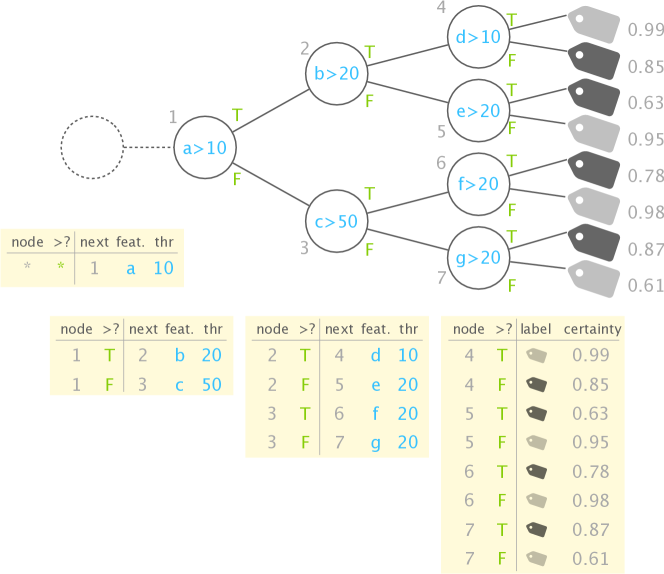
Figure 4. Encoding $\boldsymbol{RFs}$ in match&action tables

Encoding context-dependent RFs  Encoding multiple context-dependent $RFs$ is analogous to encoding one $RF$ as described above. It does not require additional tables because only one $RF$ is applied to each packet. pForest uses a table to map the current flow’s packet count to the applicable $RF$ for that phase.

5.3. Allocating feature memory

pForest applies two techniques in order to dynamically allocate the optimal number of bits for each feature despite the fact that P4${}_{\text{}}$ does not support dynamic memory management: (i) it adjusts the precision with which it stores each feature depending on the $RFs$; and (ii) it concatenates all required features into one bitstring.

Allocating the optimal number of bits per feature  $RFs$ do not require the absolute value of a feature. Instead, they only depend on the result of comparing feature values with thresholds. pForest leverages this for saving memory by reducing the precision and the range of the stored features in a way that allows precise comparisons with the thresholds in all models.

For positive feature values with strictly positive thresholds, and a given minimum comparison accuracy $a$, the minimum needed amount of bits $b$ is

(1) $$b=\left\lfloor{\log_{2}{\frac{2\cdot t_{max}}{t_{min}\cdot 0.5\cdot a}}}\right\rfloor+1$$

where $t_{max}$ and $t_{min}$ are the maximum and minimum thresholds with which the feature is compared. Accordingly, the amount of bits by which the feature in P4 needs to be shifted is

(2) $$s=\left\lfloor{\log_{2}{t_{min}\cdot 0.5\cdot a}}\right\rfloor$$

For counter features it holds that $a=1$ and $t_{min}=1$ because they are integers and need to be able to count from $1$. If several $RFs$ use the same features, the maximum and minimum thresholds are computed over all of them.

Example: If $RF_{3}$ and $RF_{5}$ (and no other $RFs$ in $\operatorname{C}$) use the average of the packet length as a feature, pForest looks for the overall maximum and minimum threshold $t_{max}$ and $t_{min}$ that could be applied to this feature in $RF_{3}$ and $RF_{5}$, as an example $1234.5$ and $67.8$. If the comparison accuracy is $0.01$, the resulting number of bits is $\left\lfloor{\log_{2}{\frac{2\cdot 1234.5}{67.8\cdot 0.5\cdot 0.01}}}\right\rfloor+1=13$.

Encoding all features in one bitstring  As explained above, pForest computes the number of bits that are required to store each feature. Instead of saving every feature in a separate register, pForest concatenates all values to one bitstring, which allows for dynamically allocating the per-flow memory and changin $RFs$ without re-compiling the program. In order to specify the location of each feature in this bitstring, pForest stores the positions (start and end index) in a register on the programmable network device.

6. ASAP Inference in the data plane

We now describe pForest’s data plane component, the runtime aspect of ASAP inference. Its code is partially automatically generated by the compiler (cf. §5). After an overview over the entire pipeline that a packet passes in a pForest device, we give special attention to how pForest extracts the features in the data plane, how it manages memory for them, and how it performs certainty-based labeling.

6.1. Pipeline overview

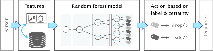
Figure 5. Packet processing pipeline in the data plane

Fig. 5 illustrates the packet processing pipeline which pForest runs in programmable network devices. Here, we summarize each processing step. The ensuing subsections provide detailed information.

Parsing  pForest extracts the Internet and transport layer header, as it contains information for some of the features. Further, it uses the 5-tuple (source IP, destination IP, source port, destination port, protocol) as an identifier for a flow.

Feature lookup  pForest computes several hashes of the flow ID and uses them to derive the storage location for the flow (§6.3.1).

Updating features  pForest computes the updated features based on the received packet (§6.2) and stores them in registers. The features are maintained in a compressed form (§6.3.2).

Applying the RF model  pForest sends the packet through the series of match&action tables which encode the $DTs$ of the $RF$ (cf.  §5). The packet count (one of the previously extracted features) determines the model used for the classification.

Deriving the label and certainty  pForest aggregates the labels (by majority-voting) and certainty scores (by summing) from the individual $DTs$ in the current $RF$ to one label and certainty.

Certainty-based labeling  pForest uses $\tau_{c}$ to determine whether it trusts the label or not, i.e., whether a definitive classification of this flow is already possible or not (§6.4).

Further actions based on label and certainty  pForest can apply arbitrary additional actions based on the label and the certainty, since this information is stored in the metadata of each packet. For example, traffic labeled as malicious could be sent to a security device for further inspection, traffic labeled as VoIP could be forwarded with higher priority, or flow IDs labeled as file transfers could be sent to a monitoring system. Adding such actions is straightforward and out of scope of this paper.

6.2. Feature extraction

pForest supports different types of features (cf.  Table 1): minimum values, maximum values, average values, counters, sums, differences and stateless metadata of the current packet. Most of them are straightforward to implement in P4${}_{\text{}}$.

However, the lack of division and floating point operations makes it challenging to compute average values. Because of this, pForest uses the exponentially weighted moving average (EWMA) as an approximation. The EWMA computes to

$${\displaystyle S_{t}={\begin{cases}Y_{1},&t=1\\ \alpha\cdot Y_{t}+(1-\alpha)\cdot S_{t-1},&t>1\end{cases}}}$$

where $S_{t}$ is the updated EWMA, $S_{t-1}$ the previous value, and $Y_{t}$ are the values to be averaged. The constant $\alpha\in[0,1]$ determines how much the current value influences the average, i.e., how fast past values are discounted. Since multiplications are not possible in many P4${}_{\text{}}$ targets, we use $\alpha=0.5$ such that multiplications can be replaced by bit shifts.

6.3. Feature memory management

We now describe how pForest solves the two challenges of dynamically and efficiently assigning (i) flows to a fixed number of memory cells, and (ii) parts of these memory cells to features.

pForest manages memory in two dimensions: per-flow memory is a bitstring of fixed size associated with each flow that pForest currently classifies. This bitstring contains per-feature memory blocks of dynamic size. Each of these blocks contains one stateful feature and pForest chooses the size of the block depending on the precision which the model requires for the respective feature (cf. §5.3).

6.3.1. Per-flow memory management

At compile time, pForest creates an array of registers to later store per-flow features. Each entry in this register contains the flow ID (a 32bit hash of the flow’s 5-tuple), the timestamp of the flow’s last packet, the packet count saying how many packets the switch received for this flow, and dynamically split space for multiple feature values.

Efficient allocation of flows to memory cells  Typically, the number of registers is much smaller than the number of possible flows (5-tuples). Since there are no linked lists or the like in P4${}_{\text{}}$, pForest implements an allocation strategy using hash-based indices.

Computing the index of a flow by using only one hash function is not efficient because of hash collisions (i.e., different flows hash to the same index). To avoid this, pForest computes multiple hashes of the flow ID using different hash functions. It then checks the register array at these indices for (I) whether it contains this flow ID; and (II) for whether its rows at these indices are usable. A row is usable if the slot is empty, or the last packet of the flow in the slot was more than a predefined timeout ago. If (I) fails, pForest uses the first-best usable row according to (II) to store the flow ID. If both conditions (I) and (II) fail, pForest cannot store stateful features and forwards the packet without classification. However, it adds a flag, which allows other devices to determine whether a flow was classified or not. That flag is stored in the Reserved Bit in the IP header. pForest implements this as a naive way of distributing the classification. More sophisticated approaches are out of scope for this paper, but we discuss ideas in §9.

6.3.2. Per-feature memory management

Besides the attributes that pForest needs to store for all random forest models (flow ID, last timestamp and packet count), pForest splits the remainder of the per-flow memory dynamically into fields in which it stores the other features. As explained in §5.3, this allows pForest to deploy a new $RF$ model based on other features without re-compiling the P4${}_{\text{}}$ program and without interrupting the network.

Concatenating all features into one bitstring and extracting them from the bitstring is possible using the bit slice operator in P4${}_{\text{16}}$, or bit shifts in P4${}_{\text{14}}$. As described in §5.3, the compiler defines the location of each feature in the bitstring and stores it in registers.

6.4. Certainty-based labeling

As described in §5.2, pForest implements $RFs$ through a series of match&action tables. They specify the feature and the threshold to compare in each node, as well as the following node depending on the result of the comparison.

Each arriving packet triggers a classification attempt of the respective flow, with the currently applicable $RF$ (if there is one, which might not be the case for the first few packets). pForest trusts the classification attempt if the certainty for the predicted label is above a threshold ($\tau_{c}$). Upon a trusted classification, pForest empties the space allocated to that flow such that it can store another flow.

7. Implementation

In this section, we outline the implementation of the training component, the data plane program, and the hardware prototype.

Feature extraction and training  Our implementation for extracting features, training context-dependent $RFs$, and compiling them to P4${}_{\text{}}$ consists of about 17 000 lines of Python code. We use dpkt (Song, 2019) for parsing network traffic and extracting features and scikit-learn (sci, 2022) for computing $RF$ models.

Inference in the data plane  The data plane component consists of about 1500 lines of P4${}_{\text{16}}$ code (for an $RF$ of 32 trees with maximum depth 10). This code runs in the behavioral model (Consortium, 2020), and we tested it using Mininet (Lantz et al., 2010).

Hardware prototype  In addition to an implementation in P4${}_{\text{16}}$, we verified that the basic operations of pForest run in real hardware. To do so, we implemented an $RF$ on Intel Tofino (Networks, 2020). Our implementation supports features of type counter (e.g., for ACK counter) and max/min (e.g., packet size) and $RFs$ up to depth 4.

8. Evaluation

In this section, we use real and synthetic datasets (§8.1) to showcase the functionality of pForest. We first confirm that the mechanisms behind ASAP inference work as intended: we show that (i) pForest’s training algorithm successfully creates context-dependent $RFs$, the offline component of ASAP inference (§8.2); and we establish that (ii) pForest successfully classifies each flow as-soon-as-possible using the certainty threshold, the online component of ASAP inference (§8.3). We also find that pForest achieves a high score both in software and hardware thanks to an accurate translation (§8.4), while it uses little memory (§8.5).

8.1. Datasets and methodology

Below, we describe each used dataset, the applied preprocessing steps, the settings for the machine learning models, and the simulation technique. We use three datasets (summarized in Table 3): a synthetic dataset that we generated ourselves and two public ones.

Synthetic dataset  The synthetic dataset consists of artificial feature values for 100’000 flows, each with nine packets. We directly generate the features for subflows $\operatorname{A}(\mathcal{F}[:i])$, $i\in{1,\ldots,9}$, and the corresponding labels with sklearn (skl, 2020a), such that different features are relevant in different phases of the flows. At packet count 4, we simulate that features ${\color[rgb]{.5,.5,.5}\mathsf{F\,1}}$ - ${\color[rgb]{.5,.5,.5}\mathsf{F\,3}}$ are redundant to the (subsequently) relevant features ${\color[rgb]{.5,.5,.5}\mathsf{F\,4}}$ - ${\color[rgb]{.5,.5,.5}\mathsf{F\,6}}$. Fig. 6 shows the relevant features for each packet of the flow. Additionally, the dataset contains 4 features which are statistically independent from the labels.

CICIDS  The CICIDS2017 dataset (Sharafaldin et al., 2018) consists of network traffic during five days and contains various attacks. Each day contains different attacks and the dataset comes with labels, which indicate the type (malicious or benign) of each flow.

UNIBS  The UNIBS-2009 dataset (of Brescia, 2009; Dusi et al., 2011; Gringoli et al., 2009) consists of network traffic from an edge router of the campus network of the University of Brescia on three consecutive days in 2009. The dataset comes with labels which indicate the protocol of each flow according to the DPI analysis by l7filter (et al., 2009).

Preprocessing  In the CICIDS dataset, we aggregated ”FTP-Patator” and ”SSH-Patator” into one attack type. In the UNIBS dataset, we ignored classes with less than $20$ samples. Here, merging is not reasonable because traffic classes represent different protocols.

Models  We used all stateful features from Table 1. In all the models, the number of trees never exceeded 32, and their depth never 20.

Simulation  §8.3 and §8.4 rely on runtime simulations of the classification, written in Python. In both sections, we compare a full-accuracy classification with a classification as it would happen in hardware (notably, without floating-point operations). In order to achieve the latter, we translate $RFs$ to their hardware counterpart, containing transformed integer thresholds with less accuracy (cf. §5.3). We also simulate the full feature extraction in hardware, including error propagation due to reduced accuracy. We then track each flow across packet counts as its features pass through the $RFs$, both for the full-accuracy and hardware mode.

Dataset	Description	PCAP Size	Flows
Synthetic
Crafted to showcase context-dependent RF		n/aa	1
CICIDS2017 (Sharafaldin et al., 2018)
Tue	FTP and SSH brute-force attacks	7.8 GB	282 418
Fri 1	botnet	8.3 GB	130 353
Fri 2	DDoS attacks	8.3 GB	114 836
Fri 3	port scan	8.3 GB	248 837
UNIBS-2009 (of Brescia, 2009)
Day 1	8 application-layer protocolsc	318 MBb	20 681
Day 2	8 application-layer protocolsc	237 MBb	19 657
Day 3	6 application-layer protocolsd	2.0 GBb	24 553
a only feature values
b packets without payload
c bittorrent, edonkey, http, imap, pop3, skype, smtp, ssl
d bittorrent, edonkey, http, pop3, skype, ssl

Table 3. Evaluation datasets

8.2. Context-dependent random forests

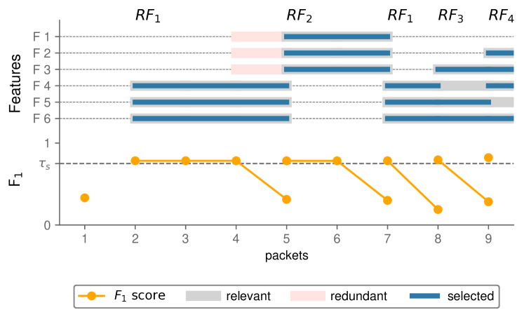
Figure 6. pForest selects relevant features and switches to a new model if the score drops below $\boldsymbol{\tau_{s}}$.

This experiment uses the synthetic dataset to show that pForest successfully implements the offline component of ASAP inference, i.e., the training of context-dependent $RFs$. The results in Fig. 6 indeed indicate that pForest (i) finds the first-possible $RF$, (ii) recycles $RFs$ as often as possible, and (iii) only selects relevant features.

First-possible RF use  pForest successfully selects the first $RF$ at packet count 2. This is the soonest a model can exceed the threshold score, according to the ASAP inference design objective.

Longest-possible RF reuse  pForest applies a found $RF$ as long as the features it uses are relevant and stable enough to allow for reusing the inferred thresholds – i.e., as long as its score is above $\tau_{s}$. Iff the features change so much that $RF_{i}$’s score is too low, pForest generates a new $RF$ (after 5, 7, 8 and 9 packets in Fig. 6). pForest successfully switches to a previously found $RF$ instead of generating a new one, if a sufficiently good one is available (here, for packet 7).

Locally minimal choice of necessary features  pForest never chooses any of the irrelevant or redundant features. Moreover, pForest only uses the necessary subset of relevant features to achieve $\tau_{s}$ (for instance, ${\color[rgb]{.5,.5,.5}\mathsf{F\,2}}$, ${\color[rgb]{.5,.5,.5}\mathsf{F\,3}}$, ${\color[rgb]{.5,.5,.5}\mathsf{F\,4}}$, ${\color[rgb]{.5,.5,.5}\mathsf{F\,6}}$ for packet count 9, even though ${\color[rgb]{.5,.5,.5}\mathsf{F\,5}}$ would also be relevant).

The efficacy of these mechanisms directly ties together with the optimization problem in §4.1 (objectives O1, O2, constraints C1, C2):

First, pForest optimizes for low memory consumption (O1): At runtime, applying the first $RF$ as soon as possible also gives the earliest-possible chance for de-allocating per-flow state after classification. Recycling $RFs$ as often as possible reduces the memory consumption of the overall $RF$ sequence; and only selecting the relevant features brings down the per-flow state.

Second, pForest’s training algorithm successfully contributes its part to maximizing classification speed (O2) by finding the first-possible $RF$. In order to allow for per-flow speed tuning at runtime, it also extracts an $RF$ sequence that can classify at later packet counts.

Third, the results inidicate that pForest’s training algorithm effectively constrains the model search with the threshold score $\tau_{s}$ (C1).

Fourth, by design, pForest allows for setting model constraints like the maximum tree depth, and only relies on features that are implementable in P4${}_{\text{}}$ to guarantee feasibility in hardware (C2).

8.3. Speed of ASAP inference at runtime

This experiment evaluates how quickly pForest classifies on a per-flow level, in terms of the packet count. We run pForest with the CICIDS and UNIBS dataset (cf. Table 3) and plot the results in Fig. 7.

The results show that pForest classifies the majority of the flows within their first few packets. In the CICIDS dataset, pForest classifies 99.1 % of the flows (Tue), 99.3 % (Fri 1), 89.3 % (Fri 2), and 82.5 % (Fri 3) after only 3 packets, with an F₁ score of 99.6 % (Tue), 99.3 % (Fri 1), 99.9 % (Fri 2), and 97.9 % (Fri 3). pForest finishes classifying all flows at 12, 16, and 10 packets with a total score of 99.6 %, 99.5 %, and 99.9 % for Tue, Fri 1 and Fri 2, respectively. For Fri 3, a small percentage (1.8 %) of flows is not classified up to a packet count of 45. In this case, the score for all classified flows is 98.2 %.

In the UNIBS dataset, pForest classifies 58.0 % (Day 1), 83.0 % (Day 2), and 66.9 % (Day 3) after 5, 5, and 7 packets with an F₁ score of 83.9 %, 87.1 % and 93.9 %, respectively. The models end up classifying 97.6 % (Day 1), 98.9 % (Day 2), and 98.6 % (Day 3) of the flows at 24, 10, and 45 packets, with a score of 84.8 %, 86.4 % and 84.1 %, respectively. This also shows that a lower $\tau_{s}$ may result in less certain decisions occurring more often, boosting the classification spread over several $RFs$.

All in all, for many of the considered datasets, one model would suffice to classify a large share of the traffic, and pForest indeed finds such a model. However, if required, pForest’s context-dependent models classify traffic in multiple stages. Day 1 of the UNIBS dataset shows such an example. There, 58.0 % of the flows are classified after 5 packets, 82.7 % after 7 packets, and 91.2 % after 10 packets. pForest therefore successfully defers uncertain decisions on a per-flow level to a later point, and indeed accepts labels when they are certain enough. This mechanism boosts the achieved overall classification score well above the threshold $\tau_{s}$. We can therefore confirm the successful interplay of context-dependent $RFs$ and certainty-based labeling, the two components of ASAP inference.

8.4. Score of ASAP inference at runtime

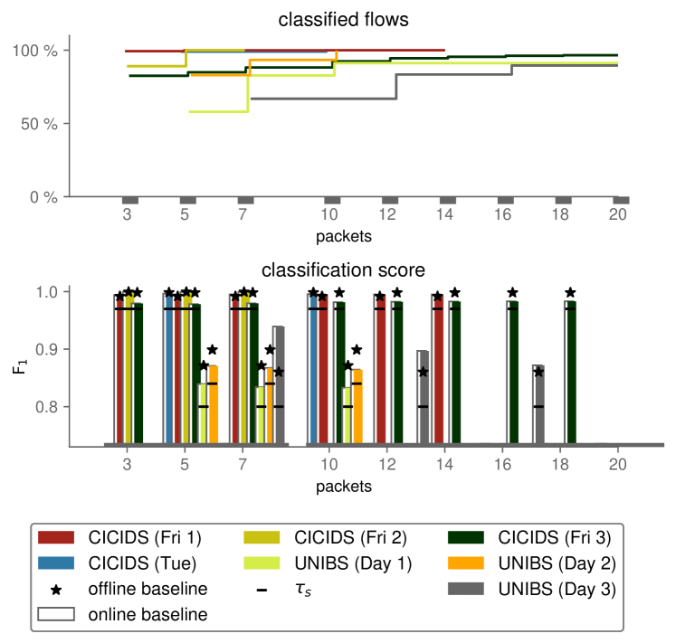
Figure 7. Percentage of classified flows and achieved accuracy. pForest classifies a large percentage of the flows after few packets with a high score (F₁ macro score over all classes).

Together with the classification speed (cf. above), we now report the achieved score for these classifications.

In this experiment, we compare pForest’s F₁ macro score over all traffic classes with an offline and an online baseline. The online baseline shows the case where the same models that pForest applies in the data plane are applied in software with floating point operations (while pForest reduces the precision of features in order to save memory and does not have floating point operations available, cf. §5). The offline baseline shows the case where the full flows are classified by a model that is trained on full flows (i.e., no ASAP classification) and with all features.

Fig. 7 visualizes the results of this experiment. We (i) compare with $\tau_{s}$ and the two baselines, (ii) discuss a general approximation of the baselines, and (iii) analyze the effect of $\tau_{c}$.

Comparison with the baselines and threshold score  We first note that pForest achieves a high score which is on-par with models running in software. pForest is never more than 0.03 % below the online baseline and never more than 7.9 % below the offline baseline. pForest exceeds the respective $\tau_{s}$ in all cases. For the CICIDS dataset, we observe that pForest is very close to the offline baseline (from 0.2 % for Fri 2 up to 2 % for Fri 3). For the CICIDS Tue, Fri 3, and UNIBS Day 1 and Day 2 datasets, there is zero difference between pForest’s inference and the online baseline; in these cases, a perfect translation was possible. For the UNIBS Day 3 dataset, pForest momentarily exceeds the offline baseline, showing that classifying subflows can actually improve the score. One possible explanation is that this is purely due to the certainty threshold, i.e., the fact that the online version only classifies a subset of flows while the offline version classifies all flows. Another possible factor could be that flows for different applications might show characteristic behavior mainly at the beginning, and that this signature fades out over time.

Arbitrary approximation of both baselines  First, pForest could approximate the offline baseline arbitrarily well: If one selects $\tau_{s}$ to be equal the offline baseline, one is guaranteed to find at the latest the offline model in the training process. Second, pForest can also approximate the online baseline by increasing the parameter for the translation precision (cf. §5.3). Trivially, this can incur a cost on the number of flows that can be stored concurrently, and on the classification speed. This highlights the trade-off of competing objectives that we laid out in the optimization problem (§4.1), namely a trade-off between classification score, memory usage, and speed.

Effect of $\boldsymbol{\tau_{c}}$  The results show that the certainty threshold allows to exceed the $\tau_{s}$ by far (e.g., 14 % for UNIBS Day 3, at packet count 7). Simultaneously, the certainty threshold allows to tune the percentage of classified flows. If $\tau_{c}$ was $0$, the overall performance would barely exceed $\tau_{s}$ since all flows (that fit into memory) would be classified with the first $RF$ in the sequence. Hence, each flow would occupy the memory for as little time as possibly achievable. Hence, varying $\tau_{c}$ over time is analogous to a control system on memory usage. pForest allows for an easy implementation of such a system via communication with the controller, since $\tau_{c}$ is adaptable at runtime. Such an extension lies beyond the scope of this paper.

8.5. Memory consumption of ASAP inference

In this experiment, we evaluate the amount of memory that pForest requires per flow in order to store its features, in dependency of different $\tau_{s}$ (Fig. 8). We again evaluate the UNIBS and CICIDS dataset.

The amount of per-flow memory consists of two parts: (i) a model-independent part for the flow ID and timestamp, requiring in 49 bits; and (ii) a model-dependent part for the feature storage.

The absolute number of bits per flow depends on the dataset and $\tau_{s}$. This is expected because depending on the dataset and $\tau_{s}$, pForest requires a different number and complexity of models.

Since a higher $\tau_{s}$ requires better models, the intuition is that this results in more features, and thus a higher memory consumption. Indeed, this is what we observe for e.g., the CICIDS Fri 1 dataset. However, interestingly, this is not the case for e.g., UNIBS Day 3.

We find that the main reason for this effect is the following: $\tau_{s}$ can be so high that one finds fewer $RFs$ that satisfy this requirement. For instance, for UNIBS Day 3, $\tau_{s}=0.6$ results in eight $RFs$ at packet counts $3,5,7,10,\ldots$ , but $\tau_{s}=0.8$ results in only four $RFs$ that are applicable at packet counts $5,7,10,22$, and $24$.

Note that since pForest relies on floating-point features, it is not possible to compare our allocation strategy with a “default” strategy for selecting the number of significant digits. Since pForest allocates the features based on the feature thresholds in the $RFs$, it is also not possible to estimate how much space non-selected features would consume if one stored them “just-in-case”.

Figure 8. Number of bits required to store per-flow features and number of trackable flows per 10MB of memory. pForest’s feature selection and optimization allows for tracking hundreds of thousands of flows per 10MB available memory.

9. Discussion

In this section, we discuss important properties, limitations and possible extensions of pForest.

Classifying other entities  In its current form, pForest classifies flows. However, the same approach works for classifying other entities (e.g., individual packets or hosts).

Resource exhaustion attacks  Because of the limited memory, pForest can only track a fixed number of concurrent flows. A malicious actor could initiate many different flows in order to exhaust the available memory. However, pForest can detect idle flows based on the timestamp of their last packet and it reuses their memory cells for another flow.

Distributing the classification  pForest implements a simple best-effort strategy to flag classified flows (cf. §6). A more sophisticated – and feasible – approach would be to actively route flows via devices that have capacity to classify them.

Other datasets  The absolute performance of pForest in terms of score and memory depends on the training dataset, but pForest computes models and feature sets that maximize the score and minimize memory requirements. Datasets can be obtained from a third party (e.g., (for Cybersecurity, 2017; ADF, 2013)) or recorded from the own network (with automated labeling (Lizhi et al., 2014; Gringoli et al., 2009)).

Different packet sampling strategies  Currently, pForest’s training algorithm creates an $RF$ sequence over sampled packet counts (at 1, 3, 5, …packets). This is just one example for a possible sampling granularity. Generally, the optimal sampling strategy depends on the available memory (since the number of $RFs$ correlates with the sampling density); the priority of classification speed; the expected variation of feature values over packet counts; constraints on the total training time; and the timing of the most relevant patterns for classification. A sampling strategy that takes all of these factors into account is an interesting avenue for future work.

10. Related work

This section compares pForest to closely related approaches. We start discussing approaches which also aim at performing inference with $RFs$ or $DTs$ on network switches before discussing other in-network machine learning approaches.

$\boldsymbol{RFs}$ and DTs on network switches  Zheng et al. and Xiong et al. have proposed several systems for $RFs$ and $DTs$ in the data plane (Xiong and Zilberman, 2019; Zheng and Zilberman, 2021; Zheng et al., 2022a, b), the most recent iteration being Ilsy (Zheng et al., 2022a) and Planter (Zheng et al., 2022b). None of these systems optimizes for early classification, unlike pForest. Indeed, Ilsy trains a single model and translates it to the data plane. Ilsy’s translation differs from pForest in that it partitions the feature space according to the subsequent trees’ decisions, and uses exact-match tables to map a flow’s feature values to the corresponding leaf node. This translation has pros and cons. On the one hand, Ilsy’s translation does not depend on the depth of the trees and, as such, it can theoretically support deeper models than pForest. On the other hand, Ilsy’s translation leads to large exact-match tables for features values that are wide-ranging. In the datasets we used for instance, some features (e.g., inter-arrival times) required more than 40 bits in the data plane.

Planter translates already-trained models and improves Ilsy’s translation strategy: It uses range-match instead of exact-match tables. This means that the feature table size now scales with the number of distinct feature thresholds used in the $RF$. However, range-match tables are located in TCAM, which is far more limited than the SRAM for exact-match tables. Since pForest generates an entire sequence of $RFs$, the number of thresholds may exceed what Planter expects to encounter: For instance, the packet length average feature for the CICIDS Tuesday dataset gets compared with a total of 5942 distinct thresholds. In contrast to Planter’s translation strategy, pForest directly stores the $RF$’s thresholds and compares the features explicitly. All in all, the best compilation strategy depends on the used features, the required model depth, and the number of thresholds per feature. It would be interesting to automatically select the best method on a case-by-case basis in future work.

Mousika (Xie et al., 2022) and (Kogan et al., 2016) compress already-trained models such that they fit into the data plane, but without optimizing for early classification, unlike pForest. That said, their compression techniques might help compressing pForest’s models further. Given its loss-freeness, (Kogan et al., 2016) compression might work out of the box on pForest model; this is not the case for Mousika though as it currently does not support stateful features.

FlowLens (Barradas et al., 2021) generates memory-efficient feature representations by aggregating them in bins and only using the most relevant bins. However, the bins’ value range corresponds to powers of 2 due to hardware restrictions. Hence, the ranges may be far off the feature threshold domains that pForest’s $RFs$ use, and therefore incur a high penalty in classification accuracy.

Homunculus (Swamy et al., 2022), pHeavy (Zhang et al., 2021), and SwitchTree (Lee and Singh, 2020) propose methods for training and translating $DTs$ or $RFs$ to the data plane.

Homunculus (Swamy et al., 2022) generates machine learning models according to hardware constraints, and translates them directly onto the switch. The authors showcase Homunculus with $RFs$. For the training, they use Bayesian optimization to explore the design space – however, they do not support generating a sequence of machine learning models. For the translation to match&action table platforms, they use Ilsy (see above). In contrast, pForest fully explores a non-sampled grid of eligible model parameters for each $RF$ meaning pForest solutions should be least as good as those found by Homunculus. In the future though, one could speed up the training process by relying on Homunculus’ strategy.

pHeavy (Zhang et al., 2021) spreads out the detection of heavy flows over several models. However, in order to confirm a flow is heavy, one needs to always apply the entire sequence. Since the models in the sequence specialize on different subsets of the training dataset, pHeavy does not attempt to reapply models for as long as possible, or to reuse them. In contrast, pForest attempts classification for all labels with each $RF$, and defers the decision only if it is uncertain.

SwitchTree (Lee and Singh, 2020) and (Xavier et al., 2021) train and implement $RFs$ or $DTs$, respectively, in switches. Unlike pForest. none of them not support early classification. Moreover, SwitchTree does not support automatic model parameter tuning.

NetPixel (Siddique et al., 2021) uses an in-switch $DT$ to classify images. Contrary to pForest, it does not classify flows, but instead performs inference on the sent data using a custom protocol.

Other in-network machine learning  Apart from $RFs$, there has been work to implement neural networks in NICs (Sanvito et al., 2018; Siracusano et al., 2018, 2022), switching chips (Siracusano and Bifulco, 2018; Qin et al., 2020; Saquetti et al., 2021), or even switches enhanced with optical matrix multiplication (Zhong et al., 2021); to translate clustering algorithms to switches (Friedman et al., 2021; Bremler-Barr et al., 2015) and to use reinforcement learning in NICs (Simpson and Pezaros, 2022). Since the best machine learning choice depends on the concrete task at hand, we view our work as complementary to these approaches. Indeed, $RFs$ have been successfully used for traffic classification (Arzani et al., 2020, 2016; Hayes and Danezis, 2016). Moreover, $RFs$ can be used for clustering (Shi and Horvath, 2006) or to approximate neural networks (Frosst and Hinton, 2017).

11. Conclusion

We presented pForest, a novel framework for performing ASAP in-network inference using $RFs$. Unlike existing in-network classifiers, pForest applies the classification after having seen the smallest amount of packets possible, and while still guaranteeing a high score. The key technical insight behind pForest is to train a sequence of $RFs$, and to automatically switch from one to the other as the flow progresses. pForest manages to optimize these models at training time according to the constraints of programmable data planes allowing them to run in existing hardware. As we show, this can be done without lowering the achieved classification score.

We implemented a prototype of pForest and showcased its practicality. Our evaluation shows that pForest manages to perform accurate ASAP classification for hundreds of thousands of flows.

Appendix A Training algorithm

The pseudocode below describes the pForest greedy algorithm (§4.3). The Python code for training consists of $\approx 17000$ lines of code, the P4 code for inference consists of $\approx 1500$ lines of code.

Input: $\mathtt{P}$, packet counts to analyse $\mathtt{F}=[\ldots,\operatorname{A}(\mathcal{F}[:p]),\ldots],p\in P$, List of features for up to p packets $\operatorname{A}(\mathcal{F})$, Features of completed flows $\mathtt{thr}$, F₁ Threshold $\text{label}(\mathcal{F})$, True labels $T$, initial trade-off parameters to select representative features

Output: $\mathtt{M}$, List of at which packet count to use what model with what features

  // ----- find redundant groups of features -----

$\operatorname{D}\leftarrow\textsc{mi\_distance}(\operatorname{A}(\mathcal{F}))$

  // information distance between features

$\mathtt{G}\leftarrow\textsc{dbscan}(distance\_matrix=\operatorname{D})$

  // redundant feature groups

$\mathtt{M}\leftarrow[]$

  // init extracted models

while $\mathtt{F}$ not empty do

      

        // ----- model search -----

       $s\leftarrow 0$

        // init score with 0

       while $\mathtt{F}$ not empty AND $s\leq\mathtt{thr}$ do

             $p\leftarrow\mathtt{P}.\text{pop}(0)$

              // get next packet count

             $f\leftarrow\mathtt{F}.\text{pop}(0)$

              // get next features

             $T\leftarrow\textsc{updateTradeOff}(T,p)$

            

              // ----- selecting representative features -----

             $f_{r}\leftarrow\textsc{representative}(\mathtt{G},T)$

            $(RF,s)\leftarrow\textsc{gridsearch}(r,\text{label}(\mathcal{F}))$

              // search for optimal RF and score

            

      if $\mathtt{F}$ is empty then

             break

      

        // ----- model optimization -----

       $f_{s}\leftarrow\textsc{SelectWithScore}(RF,f_{r},\mathtt{thr})$

        // select minimal features and retrain RF

       $f_{names}\leftarrow f_{s}.\text{names}$

        // get best feature names

       $T\leftarrow\textsc{updateUtility}(T,f_{names})$

        // increase likelihood of reselection

       $RF_{p}\leftarrow RF$

      $\mathtt{M}.\text{append}([p,RF_{p},f_{names}])$

      

        // ----- longest-possible model reapplication -----

       while $\mathtt{F}$ not empty AND $s>\mathtt{thr}$ do

             $p\leftarrow\mathtt{P}.\text{pop}(0)$

              // get next packet count

             $f\leftarrow\mathtt{F}.\text{pop}(0)$

              // get next features

             $f_{s}\leftarrow f.\text{keep}(f_{names})$

              // keep best features

            

            $s\leftarrow\textsc{score}(RF_{p},f_{s},\text{label}(\mathcal{F}))$

            if $s\leq\mathtt{thr}$ then

                   $RF_{old},f_{names\_old},s_{M}\leftarrow\textsc{BestOldRF}(\mathtt{M})$

                  if $s_{M}>\mathtt{thr}$ then

                         $RF_{p},f_{names}\leftarrow(RF_{old},f_{names\_old})$

                          // reuse old RF

                         $\mathtt{M}.\text{append}([p,RF_{p},f_{names}])$

                  else

                         $\mathtt{P}.\text{insert}(0,p)$

                          // reinsert current count at index 0

                         $\mathtt{F}.\text{insert}(0,f)$

                          // reinsert current features at index 0

                        

Algorithm 1 The pForest greedy algorithm

References

- (1)
- ADF (2013) 2013. ADFA IDS Datasets. https://research.unsw.edu.au/projects/adfa-ids-datasets.
- P41 (2018) 2018. P4-16 ~ Language Specification. https://p4.org/p4-spec/docs/P4-16-v1.1.0-spec.html.
- skl (2020a) 2020a. sklearn.datasets.make_classification. https://scikit-learn.org/stable/modules/generated/sklearn.datasets.make_classification.html.
- skl (2020b) 2020b. sklearn.metrics.f1_score. https://scikit-learn.org/stable/modules/generated/sklearn.metrics.f1_score.html.
- sci (2022) 2022. scikit-learn: machine learning in Python. https://scikit-learn.org.
- Analysis (2020) Center for Applied Internet Data Analysis. 2020. The CAIDA Anonymized Internet Traces Dataset 2008 - Ongoing.
- Arzani et al. (2016) Behnaz Arzani, Selim Ciraci, Boon Thau Loo, Assaf Schuster, and Geoff Outhred. 2016. Taking the Blame Game out of Data Centers Operations with NetPoirot. In Proceedings of the 2016 ACM SIGCOMM Conference. ACM, Florianopolis Brazil, 440–453. https://doi.org/10.1145/2934872.2934884
- Arzani et al. (2020) Behnaz Arzani, Selim Ciraci, Stefan Saroiu, Alec Wolman, Jack W Stokes, Geoff Outhred, and Lechao Diwu. 2020. PrivateEye: Scalable and Privacy-Preserving Compromise Detection in the Cloud. In 17th USENIX Symposium on Networked Systems Design and Implementation (NSDI 20). 797–815.
- Barradas et al. (2021) Diogo Barradas, Nuno Santos, Luis Rodrigues, Salvatore Signorello, Fernando M. V. Ramos, and André Madeira. 2021. FlowLens: Enabling Efficient Flow Classification for ML-based Network Security Applications. In Proceedings 2021 Network and Distributed System Security Symposium. Internet Society, Virtual. https://doi.org/10.14722/ndss.2021.24067
- Bernaille et al. (2006a) Laurent Bernaille, Renata Teixeira, Ismael Akodkenou, Augustin Soule, and Kave Salamatian. 2006a. Traffic Classification on the Fly. ACM SIGCOMM Computer Communication Review 36, 2 (April 2006), 23–26. https://doi.org/10.1145/1129582.1129589
- Bernaille et al. (2006b) Laurent Bernaille, Renata Teixeira, and Kave Salamatian. 2006b. Early Application Identification. In Proceedings of the 2006 ACM CoNEXT Conference on - CoNEXT ’06. ACM Press, Lisboa, Portugal. https://doi.org/10.1145/1368436.1368445
- Biau et al. (2019) Gérard Biau, Erwan Scornet, and Johannes Welbl. 2019. Neural Random Forests. Sankhya A 81, 2 (Dec. 2019), 347–386. https://doi.org/10.1007/s13171-018-0133-y
- Bosshart et al. (2014) Pat Bosshart, Dan Daly, Glen Gibb, Martin Izzard, Nick McKeown, Jennifer Rexford, Cole Schlesinger, Dan Talayco, Amin Vahdat, George Varghese, and David Walker. 2014. P4: Programming Protocol-Independent Packet Processors. ACM SIGCOMM Computer Communication Review 44, 3 (July 2014), 87–95. https://doi.org/10.1145/2656877.2656890
- Bremler-Barr et al. (2015) Anat Bremler-Barr, Yotam Harchol, David Hay, and Yacov Hel-Or. 2015. Ultra-Fast Similarity Search Using Ternary Content Addressable Memory. In Proceedings of the 11th International Workshop on Data Management on New Hardware. ACM, Melbourne VIC Australia. https://doi.org/10.1145/2771937.2771938
- Consortium (2020) The P4 Language Consortium. 2020. P4 bmw2 behavioral model. https://github.com/p4lang/behavioral-model.
- Daly and Cascaval (2017) Dan Daly and Calin Cascaval. 2017. P4 Architectures. https://opennetworking.org/wp-content/uploads/2020/12/p4-ws-2017-p4-architectures.pdf.
- Doshi et al. (2018) Rohan Doshi, Noah Apthorpe, and Nick Feamster. 2018. Machine Learning DDoS Detection for Consumer Internet of Things Devices. In 2018 IEEE Security and Privacy Workshops (SPW). 29–35. https://doi.org/10.1109/SPW.2018.00013
- Dusi et al. (2011) Maurizio Dusi, Francesco Gringoli, and Luca Salgarelli. 2011. Quantifying the Accuracy of the Ground Truth Associated with Internet Traffic Traces. Computer Networks 55, 5 (April 2011), 1158–1167. https://doi.org/10.1016/j.comnet.2010.11.006
- Ester et al. (1996) Martin Ester, Hans-Peter Kriegel, and Xiaowei Xu. 1996. A Density-Based Algorithm for Discovering Clusters in Large Spatial Databases with Noise. (1996).
- et al. (2009) Justin Levandoski et al. 2009. L7-Filter: Application Layer Packet Classifier for Linux. http://l7-filter.sourceforge.net/.
- for Cybersecurity (2017) Canadian Institute for Cybersecurity. 2017. Intrusion Detection Evaluation Dataset (CIC-IDS2017). https://www.unb.ca/cic/datasets/ids-2017.html.
- Formby et al. (2016) David Formby, Preethi Srinivasan, Andrew Leonard, Jonathan Rogers, and Raheem Beyah. 2016. Who’s in Control of Your Control System? Device Fingerprinting for Cyber-Physical Systems. In Proceedings 2016 Network and Distributed System Security Symposium. Internet Society, San Diego, CA. https://doi.org/10.14722/ndss.2016.23142
- Friedman et al. (2021) Roy Friedman, Or Goaz, and Ori Rottenstreich. 2021. Clustreams: Data Plane Clustering. In Proceedings of the ACM SIGCOMM Symposium on SDN Research (SOSR). Association for Computing Machinery, New York, NY, USA, 101–107.
- Frosst and Hinton (2017) Nicholas Frosst and Geoffrey Hinton. 2017. Distilling a Neural Network Into a Soft Decision Tree.
- Gómez Sena and Belzarena (2009) Gabriel Gómez Sena and Pablo Belzarena. 2009. Early Traffic Classification Using Support Vector Machines. In Proceedings of the 5th International Latin American Networking Conference on - LANC ’09. ACM Press, Pelotas, Brazil. https://doi.org/10.1145/1636682.1636693
- Gringoli et al. (2009) F. Gringoli, Luca Salgarelli, M. Dusi, N. Cascarano, F. Risso, and k. c. claffy. 2009. GT: Picking up the Truth from the Ground for Internet Traffic. ACM SIGCOMM Computer Communication Review 39, 5 (Oct. 2009), 12–18. https://doi.org/10.1145/1629607.1629610
- Hayes and Danezis (2016) Jamie Hayes and George Danezis. 2016. K-Fingerprinting: A Robust Scalable Website Fingerprinting Technique. 25th USENIX Security Symposium (USENIX Security 16) (2016), 1187–1203.
- Ho (1995) Tin Kam Ho. 1995. Random Decision Forests. In Proceedings of 3rd International Conference on Document Analysis and Recognition, Vol. 1. 278–282 vol.1. https://doi.org/10.1109/ICDAR.1995.598994
- Hullar et al. (2011) Bela Hullar, Sandor Laki, and Andras Gyorgy. 2011. Early Identification of Peer-to-Peer Traffic. In 2011 IEEE International Conference on Communications (ICC). https://doi.org/10.1109/icc.2011.5963023
- Jin et al. (2017) Xin Jin, Xiaozhou Li, Haoyu Zhang, Robert Soulé, Jeongkeun Lee, Nate Foster, Changhoon Kim, and Ion Stoica. 2017. NetCache: Balancing Key-Value Stores with Fast In-Network Caching. In Proceedings of the 26th Symposium on Operating Systems Principles. ACM, Shanghai China, 121–136. https://doi.org/10.1145/3132747.3132764
- Kogan et al. (2016) Kirill Kogan, Sergey I. Nikolenko, Ori Rottenstreich, William Culhane, and Patrick Eugster. 2016. Exploiting Order Independence for Scalable and Expressive Packet Classification. IEEE/ACM Transactions on Networking 24, 2 (April 2016), 1251–1264. https://doi.org/10.1109/TNET.2015.2407831
- Lantz et al. (2010) Bob Lantz, Brandon Heller, and Nick McKeown. 2010. A Network in a Laptop: Rapid Prototyping for Software-Defined Networks. In Proceedings of the Ninth ACM SIGCOMM Workshop on Hot Topics in Networks - Hotnets ’10. ACM Press, Monterey, California. https://doi.org/10.1145/1868447.1868466
- Lashkari (2022) Arash Habibi Lashkari. 2022. Ahlashkari/CICFlowMeter. https://github.com/ahlashkari/CICFlowMeter.
- Lee and Singh (2020) Jong-Hyouk Lee and Kamal Singh. 2020. SwitchTree: In-Network Computing and Traffic Analyses with Random Forests. Neural Computing and Applications (Nov. 2020). https://doi.org/10.1007/s00521-020-05440-2
- Lizhi et al. (2014) Peng Lizhi, Zhang Hongli, Yang Bo, Chen Yuehui, and Wu Tong. 2014. Traffic Labeller: Collecting Internet Traffic Samples with Accurate Application Information. China Communications 11, 1 (Jan. 2014), 69–78. https://doi.org/10.1109/CC.2014.6821309
- Louppe (2015) Gilles Louppe. 2015. Understanding Random Forests: From Theory to Practice.
- Meidan et al. (2017) Yair Meidan, Michael Bohadana, Asaf Shabtai, Juan David Guarnizo, Martín Ochoa, Nils Ole Tippenhauer, and Yuval Elovici. 2017. ProfilIoT: A Machine Learning Approach for IoT Device Identification Based on Network Traffic Analysis. In Proceedings of the Symposium on Applied Computing. ACM, Marrakech Morocco, 506–509. https://doi.org/10.1145/3019612.3019878
- Networks (2020) Barefoot Networks. 2020. Barefoot Tofino. https://www.barefootnetworks.com/products/brief-tofino/.
- of Brescia (2009) University of Brescia. 2009. The UNIBS Anonymized 2009 Internet Traces.
- Qin et al. (2020) Qiaofeng Qin, Konstantinos Poularakis, Kin K. Leung, and Leandros Tassiulas. 2020. Line-Speed and Scalable Intrusion Detection at the Network Edge via Federated Learning. In 2020 IFIP Networking Conference (Networking). 352–360.
- Sanvito et al. (2018) Davide Sanvito, Giuseppe Siracusano, and Roberto Bifulco. 2018. Can the Network Be the AI Accelerator?. In Proceedings of the 2018 Morning Workshop on In-Network Computing. ACM, Budapest Hungary, 20–25. https://doi.org/10.1145/3229591.3229594
- Saquetti et al. (2021) Mateus Saquetti, Ronaldo Canofre, Arthur F. Lorenzon, Fábio D. Rossi, José Rodrigo Azambuja, Weverton Cordeiro, and Marcelo C. Luizelli. 2021. Toward In-Network Intelligence: Running Distributed Artificial Neural Networks in the Data Plane. IEEE Communications Letters (2021). https://doi.org/10.1109/LCOMM.2021.3108940
- Schuster and Tromer (2017) Roei Schuster and Eran Tromer. 2017. Beauty and the Burst: Remote Identification of Encrypted Video Streams. 26th USENIX Security Symposium (USENIX Security 17) (2017), 1357–1374.
- Seals (2017) Tara Seals. 2017. Pulse-Wave DDoS Attacks Mark a New Tactic in Q2. https://www.infosecurity-magazine.com/news/pulsewave-ddos-attacks-mark-q2/.
- Sharafaldin et al. (2018) Iman Sharafaldin, Arash Habibi Lashkari, and Ali A. Ghorbani. 2018. Toward Generating a New Intrusion Detection Dataset and Intrusion Traffic Characterization:. In Proceedings of the 4th International Conference on Information Systems Security and Privacy. SCITEPRESS - Science and Technology Publications, Funchal, Madeira, Portugal, 108–116. https://doi.org/10.5220/0006639801080116
- Shi and Horvath (2006) Tao Shi and Steve Horvath. 2006. Unsupervised Learning With Random Forest Predictors. Journal of Computational and Graphical Statistics 15, 1 (March 2006), 118–138. https://doi.org/10.1198/106186006X94072
- Siddique et al. (2021) Hisham Siddique, Miguel Neves, Carson Kuzniar, and Israat Haque. 2021. Towards Network-accelerated ML-based Distributed Computer Vision Systems. In 2021 IEEE 27th International Conference on Parallel and Distributed Systems (ICPADS). 122–129. https://doi.org/10.1109/ICPADS53394.2021.00021
- Simpson and Pezaros (2022) Kyle A Simpson and Dimitrios P Pezaros. 2022. Revisiting the Classics: Online RL in the Programmable Dataplane. NOMS 2022-2022 IEEE/IFIP Network Operations and Management Symposium (2022).
- Siracusano and Bifulco (2018) Giuseppe Siracusano and Roberto Bifulco. 2018. In-Network Neural Networks.
- Siracusano et al. (2022) Giuseppe Siracusano, Salvator Galea, Davide Sanvito, and Mohammad Malekzadeh. 2022. Re-Architecting Traffic Analysis with Neural Network Interface Cards. In 19th USENIX Symposium on Networked Systems Design and Implementation (NSDI 22). 513–533.
- Siracusano et al. (2018) Giuseppe Siracusano, Davide Sanvito, Salvator Galea, and Roberto Bifulco. 2018. Deep Learning Inference on Commodity Network Interface Cards. Proc. Workshop Syst. ML Open Source Softw. NeurIPS (2018).
- Song (2019) Dug Song. 2019. dpkt. https://dpkt.readthedocs.io/.
- Swamy et al. (2022) Tushar Swamy, Annus Zulfiqar, Luigi Nardi, Muhammad Shahbaz, and Kunle Olukotun. 2022. Homunculus: Auto-Generating Efficient Data-Plane ML Pipelines for Datacenter Networks. (June 2022). https://doi.org/10.48550/arXiv.2206.05592
- Ðukic et al. (2019) Vojislav Ðukic, Sangeetha Abdu Jyothi, Bojan Karlaš, Muhsen Owaida, Ce Zhang, and Ankit Singla. 2019. Is Advance Knowledge of Flow Sizes a Plausible Assumption? 16th USENIX Symposium on Networked Systems Design and Implementation (NSDI 19) (2019), 565–580.
- Xavier et al. (2021) Bruno Missi Xavier, Rafael Silva Guimarães, Giovanni Comarela, and Magnos Martinello. 2021. Programmable Switches for In-Networking Classification. In IEEE INFOCOM 2021 - IEEE Conference on Computer Communications. https://doi.org/10.1109/INFOCOM42981.2021.9488840
- Xie et al. (2022) Guorui Xie, Qing Li, Yutao Dong, Guanglin Duan, Yong Jiang, and Jingpu Duan. 2022. Mousika: Enable General In-Network Intelligence in Programmable Switches by Knowledge Distillation. In IEEE INFOCOM 2022 - IEEE Conference on Computer Communications. 1938–1947. https://doi.org/10.1109/INFOCOM48880.2022.9796936
- Xiong and Zilberman (2019) Zhaoqi Xiong and Noa Zilberman. 2019. Do Switches Dream of Machine Learning?: Toward In-Network Classification. In Proceedings of the 18th ACM Workshop on Hot Topics in Networks. ACM, Princeton NJ USA, 25–33. https://doi.org/10.1145/3365609.3365864
- Zhang et al. (2021) Xiaoquan Zhang, Lin Cui, Fung Po Tso, and Weijia Jia. 2021. pHeavy: Predicting Heavy Flows in the Programmable Data Plane. IEEE Transactions on Network and Service Management 18, 4 (Dec. 2021), 4353–4364. https://doi.org/10.1109/TNSM.2021.3094514
- Zheng et al. (2022a) Changgang Zheng, Zhaoqi Xiong, Thanh T. Bui, Siim Kaupmees, Riyad Bensoussane, Antoine Bernabeu, Shay Vargaftik, Yaniv Ben-Itzhak, and Noa Zilberman. 2022a. IIsy: Practical In-Network Classification.
- Zheng et al. (2022b) Changgang Zheng, Mingyuan Zang, Xinpeng Hong, Riyad Bensoussane, Shay Vargaftik, Yaniv Ben-Itzhak, and Noa Zilberman. 2022b. Automating In-Network Machine Learning.
- Zheng and Zilberman (2021) Changgang Zheng and Noa Zilberman. 2021. Planter: Seeding Trees within Switches. In Proceedings of the SIGCOMM ’21 Poster and Demo Sessions (SIGCOMM ’21). Association for Computing Machinery, New York, NY, USA, 12–14. https://doi.org/10.1145/3472716.3472846
- Zhong et al. (2021) Zhizhen Zhong, Weiyang Wang, Manya Ghobadi, Alexander Sludds, Ryan Hamerly, Liane Bernstein, and Dirk Englund. 2021. IOI: In-network Optical Inference. In Proceedings of the ACM SIGCOMM 2021 Workshop on Optical Systems. ACM, Virtual Event USA, 18–22. https://doi.org/10.1145/3473938.3474508