Lead-Lag-Shaped Interactive Force Estimation by Equivalent Output Injection of Sliding-Mode

Abstract

Estimation of interactive forces, which are mostly unavailable for direct measurement on the interface between a system and its environment, is an essential task in various motion control applications. This paper proposes an interactive force estimation method, based on the well-known equivalent output injection of the second-order sliding mode. The equivalent output injection is used to obtain a frequency-unshaped quantity that appears as a matched external disturbance and encompasses the interactive forces. Afterwards, a universal lead-lag shaper, depending on dynamics of the motion control system coupled with its environment, is used to extract an interactive force quantity. Once identified, the lead-lag shaper can be applied to the given system structure. An experimental case study, using a valve-controlled hydraulic cylinder counteracted by the dynamic load, is demonstrated with an accurate estimation of the interactive force, that in comparison to the reference measurement.

I INTRODUCTION AND BACKGROUND

Motion control applications are often dealing with weakly known interactive forces, which directly affect the controlled system performance and can, in worst case, even provoke instabilities. The control technologies, where complying forces between the system and its environment are crucial for a predefined and safe operation, range from the nanoscale touching devices [1] and medical mechatronics [2, 3] to the humanoid-like [4, 5] and industrial [6] robotics, equally as bulky hydraulic systems [7, 8], here just to refer to some of them. While structural differences between the motion- and force-controlled systems and their relationship to mechanical impedance [9], by interaction with environment, have been highlighted in an elegant way in [10], the issues related to coupling of the interactive forces proved to be challenging. This is especially when shaping the desired endpoint impedance in the real-world servo-systems, see e.g. [11]. Besides, more recent experimental studies, e.g. [12] in robotics, demonstrate that an accurate and robust estimation of the contact, correspondingly external, forces and torques remains a non-trivial task, even for relatively simple (that case rigid) environmental couplings and specific tuning of the modeled disturbance dynamics.

I-A Interaction with environment

For analyzing couplings of an interactive force, occurring on the environmental interface, consider a generic two-port representation $\mathbf{S}$ of the actuated motion system (i.e. servomechanism) which interacts with its environment, see block diagram shown in Fig. 1. Recall that the two-port models, correspondingly networks, with the associated effort $(F_{1},F_{2})$ and flow $(V_{1},V_{2})$ variables, and their product representing the instantaneous input and output power and, hence, energy transfer, are particulary useful for modeling interaction between servomechanisms and environments. That allows specifying a mechanical impedance and designing an impedance controller [9] which, when has a varying closed-loop stiffness, can be seen as a general form of the motion control [10].

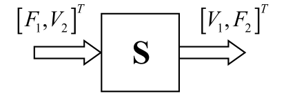
Figure 1: Generic two-port of servomechanism with its environment.

Considering, in the most simple case, a linear two-port model of an interactive motion system (cf. Fig. 1), one can recognize that the $2\times 2$ square matrix $\mathbf{S}$ will contain the transfer functions relating to each other the velocity and force at each port, cf. [11]. It is evident that while $S_{ii}$ describe the transfer characteristics of a servomechanism and environment, correspondingly, the $S_{ij}$ transfer functions with $i\neq j$ are responsible for the cross-couplings between both. Assuming $i=1,2$ for the servomechanism and environment, respectively, and $\mathbf{S}$ to be regular in terms of invertibility, one can write

$$\left[\begin{array}[]{c}F_{1}\\ V_{2}\\ \end{array}\right]=\mathbf{S}^{-1}\left[\begin{array}[]{c}V_{1}\\ F_{2}\\ \end{array}\right]$$ (1)

for reverse transfer characteristics of the coupled interactive system. Introducing $\bar{\mathbf{S}}\equiv\mathbf{S}^{-1}$, one can recognize that the forces of the servomechanism and environmental are additionally balanced by the rate of induced relative motion, meaning $F_{1}=\bar{S}_{12}F_{2}+\bar{S}_{11}V_{1}$. It is evident that an unconstrained relative motion, i.e. $\bar{S}_{12}\,\vee\,F_{2}=0$, allows to determine the flow quantity of servomechanisms from its effort counterpart and vice versa. As implication, the forward transfer function $\bar{S}_{11}$ is mostly assumed to be known, correspondingly identified, for the used nominal servomechanism. On the contrary, the cross-coupling transfer characteristics $\bar{S}_{12}$ of environmental interconnection can be barely available and, as implication, hinder the estimation of external effort variables. Therefore, an appropriate estimation, or approximation, of the environmental couplings can be crucial for properly reconstructing the interactive forces which affect the overall controlled system.

Since an interface between the system and its environment is application-specific, in the most cases, a suitable reshaping of the interactive force estimate is required, once the effort variable $F_{2}$ is of a primary interest. It is worth noting that in the most simple case of a directly matched interactive force (here one can think on an absolutely rigid manipulator hitting a stiff obstacle with unity restitution coefficient and zero damping) $\bar{S}_{12}$ will yield the unity or constant transfer characteristics. On the other hand, when thinking about a standard solid (also called Zener) model of the viscoelastic type, see e.g. [13] for fundamentals, one can assume

$$\bar{S}_{12}(s)=a\,\frac{b\,s+1}{c\,s+1},$$

where $a,\,b,\,c>0$ coefficients bear the corresponding elasticity and viscosity constants of the associated environment. Obviously $s$ is the Laplace variable of the transfer function. One can recognize that the above transfer function coincides with the lead or lag element, for $c<b$ or $c>b$ respectively. With the same line of argumentation, various structural properties of environmental interfaces, like for example thermo-rheological, creeping and relaxation, equally as visco-elasto-plastic effects, can be incorporated into shaping the external interactive forces. In general, we assume a generic lead-lag shaper

$$\bar{S}_{12}(s)=a\,\prod_{k=1}^{n}\frac{b_{k}\,s+1}{c_{k}\,s+1},$$ (2)

with $a>0$ and $b_{k},\,c_{k}\geq 0$, while the lead-lag order $n\geq 1$ is the free structural parameter, depending on principles and mechanisms of the interactive force couplings.

I-B Contribution and structure of the paper

This paper is contributing to robust estimation of the interactive forces, associated with environmental impact and constrained response, when no explicit parametric modeling of the environment interface is provided. The principal structural properties of an interactive force, which is back-propagated to the actuator dynamics of controlled motion system, are assumed as general lead-lag characteristics, cf. Section I-A. The corresponding order of the lead-lag shaper is understood to be rather case-specific, that means depending on the principal behavior of both, motion control system and its environment. The proposed method relies on the so-called equivalent output injection, see e.g. [14, 15] for details, of the second-order sliding mode [16, 17]. Recall that the latter is robust to the unknown bounded perturbations, has a finite-time convergence property, and is suitable for using the single output of second-order systems, for maintaining those in the sliding-mode. It should also be noted that an equivalent approach, but involving more detailed explicit modeling of nominal system dynamics, has been recently shown [18] for the same experimental data.

Following assumptions are made for the rest of the paper. (i) a time-continuous system dynamics is uniformly considered, despite all real-time implementations are using the forward Euler discretization scheme. (ii) initial conditions are negligible so that the transient phases, equally as convergence phase to the sliding-mode, are taken out evaluation, correspondingly performance assessment. (iii) neither noise by-effects nor sliding-mode related chattering are within the scope of the recent work and, therefore, neglected in both the analysis and experimental evaluation. (iv) for the sake of generality, especially in relation to a robust shaper design in frequency-domain and lack of an accurate friction identification (see e.g. [19] for more details on frictional uncertainties) the dynamic friction effects are taken out of consideration.

The main content of the paper is organized as follows. In Section II the second-order sliding mode, correspondingly the associated exact differentiator, are summarized for the sake of clarity. An optimal parameter setting, according to [20], is briefly addressed. The proposed estimation of interactive forces is described in Section III, together with the corresponding lead-lag shaping of equivalent output injection. An experimental case study, dedicated to predicting the interactive load forces in a controlled hydraulic cylinder system, is provided in Section IV. The paper is concluded by Section V.

II SECOND-ORDER SLIDING MODE

The so-called second-order sliding mode, see e.g. [16, 17] for fundamentals, appears when a sliding variable $\sigma$ satisfies

$$\sigma=\dot{\sigma}=0,$$ (3)

while $\sigma=\sigma(t,\mathbf{x})\in\mathbb{R}$ is a sufficiently smooth function of time $t$ and system states $\mathbb{x}$, and understood in the Filippov sense [21]. The main issue with using higher (than first) order sliding modes is the demand on system states to be available, correspondingly measurable. This means for fulfilling (3), both $\sigma$ and $\dot{\sigma}$ should be determinable as from the system states, cf. with Chapter 3 in [16]. Single exception is the well-known super-twisting algorithm (STA) [24] which needs the measurement of $\sigma$ only, for steering the system into the second-order sliding mode. STA drives both $\sigma,\,\dot{\sigma}\rightarrow 0$ in finite time, so that a second-order sliding mode occurs after the system reaches the globally stable origin $(\sigma,\,\dot{\sigma})=\mathbf{0}$.

Based thereupon, the first-order robust differentiator, introduced by Levant in [25], can be written as

$$\dot{\hat{x}}_{1} = K_{1}\sqrt{|e|}\,|e|^{-1}e+\hat{x}_{2},$$ (4)

$$\dot{\hat{x}}_{2} = K_{2}\,|e|^{-1}e.$$ (5)

It aims at providing an exact estimation of unavailable $\dot{\sigma}(t>T)\equiv\hat{x}_{2}$ quantity, after a finite convergence time $T>0$. The estimator dynamics, given by (4), (5), is driven by the output error $e=\sigma-\hat{x}_{1}$, while only the sliding variable $\sigma(t)$ is available from the system measurements. For the appropriately chosen estimator gains $K_{1},K_{2}>0$, which are the STA parameters [25], the robust exact differentiator ensures convergence of the states estimation, i.e. $e=\dot{e}=0$, and that after finite-time transients. This is generally valid for an upper bounded second-order dynamics, where $|\ddot{\sigma}|\leq L=\mathrm{const}<\infty$ denotes the Lipschitz constant to be known. The positive constant $L$ is understood to upper bound the matched, but unknown, disturbances of the nominal second-order dynamics.

For an optimal STA gain setting, one can assume

$$K_{1}=2.028\sqrt{K_{2}},\quad K_{2}=1.1L,$$ (6)

as has been described and analyzed in detail in [20]. Here is is worth noting that the STA gain setting (6) aims for minimizing the amplitude of fast oscillations, i.e. amplitude of chattering, in the closed-loop of STA estimator. Further, one can notice that the above $K_{2}$-selection, with respect to $L$, is the standard one, also for the HOSM derivatives, as initially proposed in [25] and later confirmed in multiple works, see e.g. [22, 26, 20]. The optimal gain setting (6) has also been recently evaluated with experiments in [27]. From the above, it is obvious that an appropriate gains assignment requires the upper bound of the disturbed second-order dynamics to be known. This is a well-known and studied issue when designing the STA-based estimators, equally as control algorithms, see e.g. [28]. If $L$ is unavailable from some nominal system description, correspondingly design, its approximative estimation is to be obtained based on the experimental data. An example of such identification approach aimed for determining $L$ is shown further on in Section IV, within the provided experimental case study.

III ESTIMATION OF INTERACTIVE FORCES

For estimating the interactive forces of environment, consider a perturbed second-order dynamic system as

$$\ddot{\sigma}=f(u,\sigma,\dot{\sigma},t)+\xi(t).$$ (7)

The unperturbed (nominal) system dynamics is captured by $f(\cdot)$, including the linear scaling factor of the inertial mass $m$. The most simple case, of an actuated unconstrained motion, one assumes $f=m^{-1}\bigl{(}u-d(\dot{\sigma})\bigr{)}$ where an available input value is equivalent to the controlled force of the servomechanism, i.e. $u\equiv F_{1}$. The induced motion dynamics is counteracted by the velocity-dependent damping $d(\cdot)$, that is (mostly) the Coulomb and/or viscous friction, both inherent for the moving bodies with bearings, correspondingly contact surfaces, of an actuated relative displacement. For a controlled servomechanism coupled with its environment, the interactive forces are provoking an unknown, yet upper bounded, perturbation $\xi(t)$. The boundedness assumption of the perturbation dynamics follows directly from the naturally limited interactive forces, for which $|F_{2}|<F_{\max}$ is guaranteed for the finite system accelerations, input excitations, and some constant $F_{\max}$. The boundedness assumption argues again in favor of the lead-lag shaped couplings with environment, cf. (2), meaning it excludes the free integrators or differentiators when determining $\bar{S}_{12}$. We also stress that due to the boundedness assumption of the perturbed second-order dynamics, the second-order sliding mode appears particulary suitable for a robust estimation of the unknown interactive forces.

For the perturbed case of an exact differentiator (4), (5) we introduce the state estimation error $\tilde{x}_{2}=\dot{\sigma}-\hat{x}_{2}$ which dynamics is, consequently, governed by

$$\dot{\tilde{x}}_{2}=f(\cdot)+\xi(t)-K_{2}\,|e|^{-1}e.$$ (8)

Note that the nominal system dynamics, here and in the following, is written without explicit arguments, this for the sake of simplicity and for not forcing oneself to have time-varying and full-state-dependent dynamics. The finite-time convergence to the second-order sliding mode set ensures that there exists a time constant $T>0$ such that for all $t\geq T$ the following identity holds $0\equiv\dot{\tilde{x}}_{2}$ [15], thus leading to

$$K_{2}\,|e|^{-1}e=f(\cdot)+\xi(t).$$ (9)

Thereupon, an equivalent output injection, cf. [15], is

$$\chi\equiv K_{2}\,\mathrm{sign}(e)=f(\cdot)+\xi(t).$$ (10)

Theoretically, an equivalent output injection is determined by an infinite switching frequency of the discontinuous term, which is maintaining the converged second-order sliding mode. It implies that the spectral distribution of equivalent output injection contains both, the known part of the motion dynamics and unknown coupled interactive forces, in addition to high-frequent oscillations of the sliding-mode known as chattering [16, 17]. Since the practical finite-sampling of an estimator (in original work [15] also called observer) produces a high but finite switching frequency, the necessity to apply a filter to $\chi$ becomes self-evident. Most simple case, a finite impulse response (FIR) unity gain low-pass filter, denoted by $h$, can be designed in frequency domain and used as a chattering cut-off operator. This, rather standard [17], filtering approach that allows using an equivalent output injection, will indispensably provoke an additional phase lag in the estimate

$$\hat{\xi}(t)\equiv h\bigl{[}\chi(t)-f(\cdot)(t)\bigr{]}=\xi(t)+\varepsilon(t).$$

Here $\varepsilon(t)$ is the dynamic perturbation difference caused by the filtering process, while $\varepsilon(s)\rightarrow 0$ for $\omega\rightarrow 0$, for $\omega$ to be the angular frequency. Therefore, the filtering by $h$ causes no errors in the lower frequencies.

Instead of low-pass filtering the equivalent output injection, we make use of the lead-lag transfer characteristics of the environmental couplings, cf. Section I-A. Without loss of generality and needs of specifying the polynomial coefficients and order of (2), we can distinguish two principally different classes of environmental interfaces – of the lead- or of the lag-type at higher angular frequencies $\omega$. While both will approach the $a$-gain at steady-state, i.e. for $\omega\rightarrow 0$, an application-specific finite gain enhancement will be otherwise expected for the lead-type interfaces at $\omega\rightarrow\infty$. Consequently logical, a lag-type environmental interface will exhibit a finite gain-reduction at high frequencies, i.e. at $\omega\rightarrow\infty$. Falling back on a viscoelasticity type interface modeling, as explained in Section I-A, some general remarks can be drawn to attention. If, during the principal behavior of environmental interface, the elasticity will be dominating over viscosity, a lag-type coupling of the interactive forces can be expected. On the contrary, a lead-type environmental coupling is to be expected when the viscosity effects on the interface dominate over elasticities in the structure. One should keep in mind that the above distinguishing between the lead- and lag-type interfaces refer to an upper bound of the excitation frequencies. At the same time, an application-specific shaping of the overall transfer characteristics of the coupling interface is required for $0<\omega<\infty$, thus giving reasoning to the generic shaper (2).

The above considerations allow for using the lead-lag shaper and, with the introduced transfer function $G(s)\equiv m\,\bar{S}_{12}^{-1}(s)$, designing an infinite impulse response (IIR) filter $g(\cdot)$, which is the inverse Laplace transform of $G$. It is worth emphasizing that the transfer characteristics, captured by $G$, do not reflect an (artificially) injected low-pass filter, but have a direct relationship to the coupling interface properties of the system $\mathbf{S}$, cf. Section I-A. Hence, the estimated interactive force can be obtained from the equivalent output injection as

$$\hat{F}_{2}(t)=g\bigl{(}K_{2}\,\mathrm{sign}(e)(t)-f(\cdot)(t)\bigr{)}.$$ (11)

An essential point, to be equally mentioned here, is that an unavailable system state can enter the nominal dynamics $f(\cdot)$. This case, the state estimate, e.g. $\hat{x}_{2}$, has to be used instead of the unmeasurable system quantity. Yet this leads to a feedback-coupled estimator dynamics and, as a logical consequence, to an additional initial perturbations $f(\hat{x}_{2})(t)-f(\dot{\sigma})(t)$ for $t<T$, i.e. before the finite-time convergence of the robust differentiator, cf. Section II. Still, when fairly requiring the boundedness of an initial state discrepancy and BIBO characteristics of the nominal dynamic map $f(\cdot)$, one can neglect the transient phase $t<T$ and assumes $f(\hat{x}_{2})\approx f(\dot{\sigma})$ $\forall\,t>T$, i.e. once the system is in sliding-mode. For the related convergence analysis and observer stability, in spite of a feedback-coupled estimation dynamics, an interested reader is referred to [29].

IV EXPERIMENTAL CASE STUDY

The experimental case study is accomplished on a valve-controlled hydraulic cylinder system, counteracted by another cylinder which appears as a dynamic system load. Both cylinders are rigidly coupled to each other via a sensing force-cell, that allows for direct reference measurement of the interactive forces which we aim to estimate, correspondingly predict. More technical details on the experimental setup of hydraulic system in use can be found in [30, 31].

The single system parameter identified prior to the experimental study is the overall lumped moving mass $m$, which appears as a scaling factor in the total force balance. Both, the shaping lead-lag dynamics

$$G(s)=1.7\,\frac{2.84\times 10^{-5}\,s+1}{0.00137\,s+1}\cdot\frac{2.38\times 10^{-5}\,s+1}{0.01284\,s+1},$$ (12)

and the unknown Coulomb friction coefficient $\gamma$, resulting in

$$f=m^{-1}\bigl{(}u-\gamma\,\mathrm{sign}(\hat{x}_{2})\bigr{)}=0.5882\bigl{(}u-160\,\mathrm{sign}(\hat{x}_{2})\bigr{)},$$ (13)

are identified simultaneously, by a standard numerical minimization routine, using the measured reference force data.

Since $L$ remains the single unknown design parameter of the STA-based estimator, the proposed approach aims at determining it via numerical optimization. That is performed on experimental data of the single measured output. Here it is worth to recall that the reference force measurement can be unavailable during the design stage. Solving minimization

$$\underset{L}{\min}\sum\limits_{i=1}^{N}e(L)^{2},$$ (14)

of the squared output error yields $L=3.1$. Here $N$ is the size of the measured and STA-estimated data, while the output error $e$ depends on the $L$-assignment affecting the STA-gains cf. (6). The cumulative squared error (14) is shown in Fig. 2 against the varying $L$, out of which an optimal $L$-value is read off.

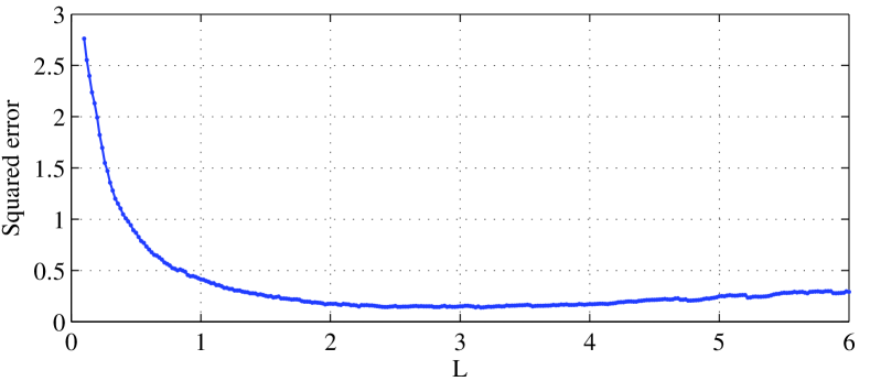
Figure 2: Cumulative squared error against varying $L$.

The reference measured interactive force, used for the above parameters identification, is shown versus the estimated one in Fig. 3. One can recognize both time series are well in accord with each other, and that for transient, oscillating, and quasi steady-state values of lower (about 1000 N) and higher (about 6000 N) amplitudes.

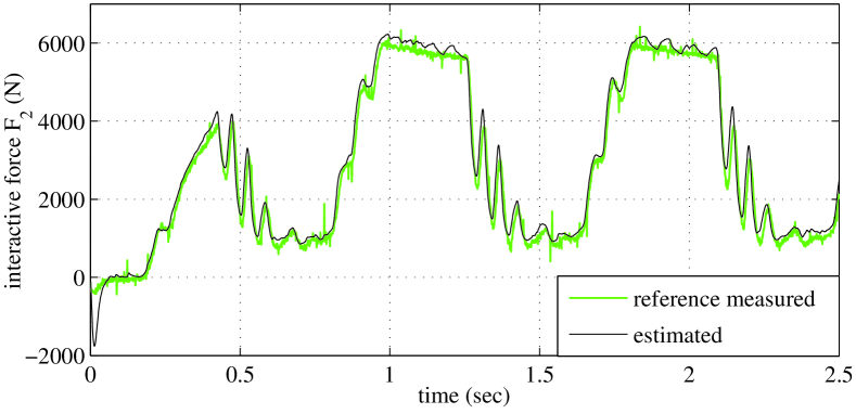
Figure 3: Estimated interactive force $\hat{F}_{2}$ versus reference measured $F_{2}$.

The corresponding motion profile, with the measured and estimated quantities of relative displacement and velocity, are shown in Fig. 4 (a) and (b) respectively. One can recognize a relatively high level of the displacement measurement noise which indirectly argues in favor of the robust sliding-mode-based estimation scheme. From Fig. 4 (b) one can further recognize, that the relative motion is with relatively low velocity amplitudes. The velocity pattern is frequently oscillating in a stick-slip manner, also with multiple sporadic zero-crossings, that is typical for slower displacements under impact of a high process noise and external perturbations, cf. Fig. 4 (a).

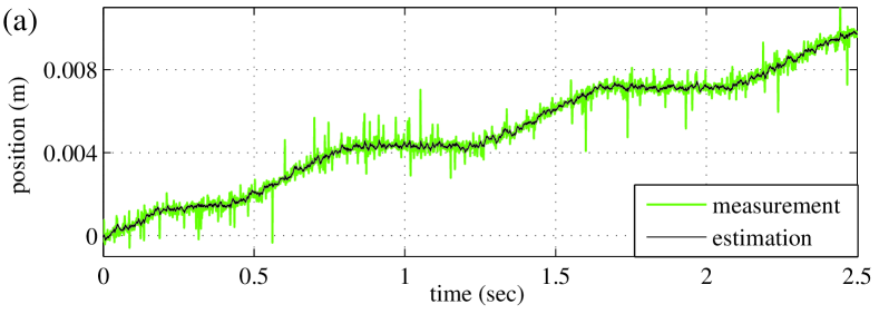
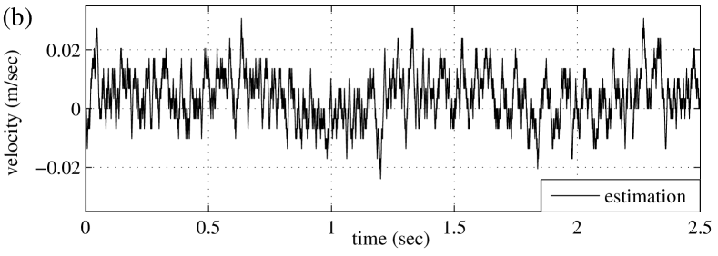
Figure 4: Trajectories of induced motion with interactive force, measured versus estimated relative displacement (a) and estimated relative velocity (b)

Another set of unseen data, i.e. not involved into parameters identification, has been equally used for evaluating the estimation of an interactive force. Here the estimated and reference measured interactive force values are shown opposite to each other in Fig. 5.

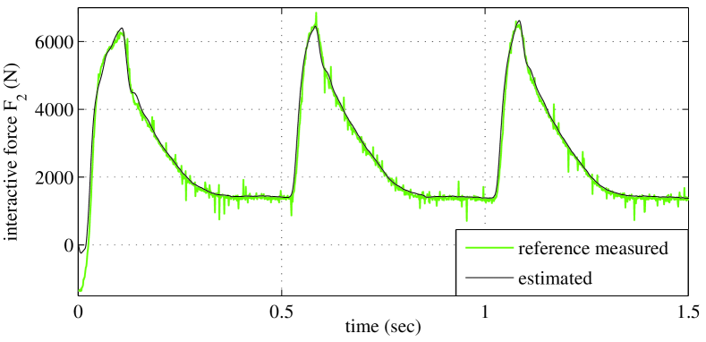
Figure 5: Estimated interactive force $\hat{F}_{2}$ versus reference measured $F_{2}$.

This time, the interactive force has more steeply periodic peaks, coming from the saw-shaped profile of the applied counteracting load, and the longer steady-state plateaus in-between, cf. Fig. 5. Also here one can recognize a good accord between the estimation and measurement.

V CONCLUSIONS

For robust estimation of the unknown interactive forces, a method based of the second-order sliding-mode and associated equivalent output injection principles has been proposed. It is shown that, depending on the system dynamics and interactive force couplings, which appear as matched perturbations, the equivalent output injection can be reshaped via the standard lead-lag transfer characteristics. Design of the estimation method is presented along with the parametrization of an exact differentiator [25] and the proposed strategy of reshaping the equivalent output injection quantity. An experimental case study, showing an accurate estimation of the interactive force in the dynamically loaded valve-controlled hydraulic cylinder with high measurement and process noise, is provided for evaluation of the proposed method.

References

- [1] M. Sitti and H. Hashimoto, “Teleoperated touch feedback from the surfaces at the nanoscale: modeling and experiments,” IEEE/ASME Trans. on Mechatronics, vol. 8, no. 2, pp. 287–298, 2003.
- [2] S. Katsura, W. Iida, and K. Ohnishi, “Medical mechatronics - an application to haptic forces,” Annual Reviews in Control, vol. 29, no. 2, pp. 237–245, 2005.
- [3] N. Zemiti, G. Morel, T. Ortmaier, and N. Bonnet, “Mechatronic design of a new robot for force control in minimally invasive surgery,” IEEE/ASME Trans. on Mechatronics, vol. 12, no. 2, pp. 143–153, 2007.
- [4] D. Prattichizzo, M. Malvezzi, M. Gabiccini, and A. Bicchi, “On motion and force controllability of precision grasps with hands actuated by soft synergies,” IEEE Trans. on Robotics, vol. 29, pp. 1440–1456, 2013.
- [5] F. Abi-Farraj, B. Henze, C. Ott, P. R. Giordano, and M. A. Roa, “Torque-based balancing for a humanoid robot performing high-force interaction tasks,” IEEE Robotics and Automation Letters, vol. 4, no. 2, pp. 2023–2030, 2019.
- [6] A. Alcocer, A. Robertsson, A. Valera, and R. Johansson, “Force estimation and control in robot manipulators,” IFAC Proceedings Volumes, vol. 36, no. 17, pp. 55–60, 2003.
- [7] N. Niksefat and N. Sepehri, “Designing robust force control of hydraulic actuators despite system and environmental uncertainties,” IEEE Control Systems Magazine, vol. 21, no. 2, pp. 66–77, 2001.
- [8] J. Koivumäki and J. Mattila, “Stability-guaranteed force-sensorless contact force/motion control of heavy-duty hydraulic manipulators,” IEEE Trans. on Robotics, vol. 31, no. 4, pp. 918–935, 2015.
- [9] N. Hogan, “Impedance control: An approach to manipulation,” Journal of dynamic systems, measurement, and control, vol. 107, no. 1, 1985.
- [10] K. Ohnishi, N. Matsui, and Y. Hori, “Estimation, identification, and sensorless control in motion control system,” Proceedings of the IEEE, vol. 82, no. 8, pp. 1253–1265, 1994.
- [11] S. P. Buerger and N. Hogan, “Complementary stability and loop shaping for improved human–robot interaction,” IEEE Trans. on Robotics, vol. 23, no. 2, pp. 232–244, 2007.
- [12] A. Wahrburg, J. Bös, K. D. Listmann, F. Dai, B. Matthias, and H. Ding, “Motor-current-based estimation of cartesian contact forces and torques for robotic manipulators and its application to force control,” IEEE Trans. on Autom. Science and Eng., vol. 15, pp. 879–886, 2018.
- [13] N. W. Tschoegl, The phenomenological theory of linear viscoelastic behavior: an introduction. Springer Science, 2012.
- [14] C. Edwards, S. K. Spurgeon, and R. J. Patton, “Sliding mode observers for fault detection and isolation,” Automatica, vol. 36, no. 4, pp. 541–553, 2000.
- [15] J. Davila, L. Fridman, and A. Poznyak, “Observation and identification of mechanical systems via second order sliding modes,” Int. Journal of Control, vol. 79, no. 10, pp. 1251–1262, 2006.
- [16] W. Perruquetti and J. P. Barbot, Sliding mode control in engineering. M. Dekker Publisher, 2002.
- [17] Y. Shtessel, C. Edwards, L. Fridman, and A. Levant, Sliding mode control and observation. Springer, 2014.
- [18] M. Ruderman, L. Fridman, and P. Pasolli, “Virtual sensing of load forces in hydraulic actuators using second- and higher-order sliding modes,” Control Engineering Practice, vol. NN, no. pp, 2019.
- [19] M. Ruderman and M. Iwasaki, “Observer of nonlinear friction dynamics for motion control,” IEEE Trans. on Industrial Electronics, vol. 62, no. 9, pp. 5941–5949, 2015.
- [20] U. P. Ventura and L. Fridman, “Design of super-twisting control gains: a describing function based methodology,” Automatica, vol. 99, pp. 175–180, 2019.
- [21] A. Filippov, Differential equations with discontinuous right-hand sides. Kluwer Academic Publishers, 1988.
- [22] A. Levant, “Higher-order sliding modes, differentiation and output-feedback control,” Int. Journal of Control, vol. 76, pp. 924–941, 2003.
- [23] E. Cruz-Zavala and J. A. Moreno, “Levant’s arbitrary order exact differentiator: A Lyapunov approach,” IEEE Trans. on Automatic Control, pp. 1–1, 2018.
- [24] A. Levant, “Sliding order and sliding accuracy in sliding mode control,” Int. Journal of Control, vol. 58, no. 6, pp. 1247–1263, 1993.
- [25] A. Levant, “Robust exact differentiation via sliding mode technique,” Automatica, vol. 34, no. 3, pp. 379–384, 1998.
- [26] M. Reichhartinger and S. Spurgeon, “An arbitrary-order differentiator design paradigm with adaptive gains,” Int. Journal of Control, vol. 91, no. 9, pp. 2028–2042, 2018.
- [27] M. Ruderman and L. Fridman, “Use of second-order sliding mode observer for low-accuracy sensing in hydraulic machines,” in IEEE 15th Int. Workshop on Variable Structure Systems and Sliding Mode Control (VSS18), 2018, pp. 315–318.
- [28] A. Levant, “Principles of 2-sliding mode design,” Automatica, vol. 43, no. 4, pp. 576–586, 2007.
- [29] J. Davila, L. Fridman, and A. Levant, “Second-order sliding-mode observer for mechanical systems,” IEEE Trans. on Automatic Control, vol. 50, no. 11, pp. 1785–1789, 2005.
- [30] P. Pasolli and M. Ruderman, “Linearized piecewise affine in control and states hydraulic system: Modeling and identification,” in IEEE 44th Annual Conference of the Industrial Electronics Society, 2018, pp. 4537–4544.
- [31] P. Pasolli and M. Ruderman, “Hybrid state feedback position-force control of hydraulic cylinder,” in IEEE Int. Conference on Mechatronics (ICM), 2019, pp. 54–59.