Sparse Deep Neural Network Graph Challenge

Abstract

The MIT/IEEE/Amazon GraphChallenge.org encourages community approaches to developing new solutions for analyzing graphs and sparse data. Sparse AI analytics present unique scalability difficulties. The proposed Sparse Deep Neural Network (DNN) Challenge draws upon prior challenges from machine learning, high performance computing, and visual analytics to create a challenge that is reflective of emerging sparse AI systems. The Sparse DNN Challenge is based on a mathematically well-defined DNN inference computation and can be implemented in any programming environment. Sparse DNN inference is amenable to both vertex-centric implementations and array-based implementations (e.g., using the GraphBLAS.org standard). The computations are simple enough that performance predictions can be made based on simple computing hardware models. The input data sets are derived from the MNIST handwritten letters. The surrounding I/O and verification provide the context for each sparse DNN inference that allows rigorous definition of both the input and the output. Furthermore, since the proposed sparse DNN challenge is scalable in both problem size and hardware, it can be used to measure and quantitatively compare a wide range of present day and future systems. Reference implementations have been implemented and their serial and parallel performance have been measured. Specifications, data, and software are publicly available at GraphChallenge.org.

I Introduction

MIT/IEEE/Amazon GraphChallenge.org encourages community approaches to developing new solutions for analyzing graphs and sparse data. GraphChallenge.org provides a well-defined community venue for stimulating research and highlighting innovations in graph and sparse data analysis software, hardware, algorithms, and systems. The target audience for these challenges any individual or team that seeks to highlight their contributions to graph and sparse data analysis software, hardware, algorithms, and/or systems.

As research in artificial neural networks progresses, the sizes of state-of-the-art deep neural network (DNN) architectures put increasing strain on the hardware needed to implement them [1, 2]. In the interest of reduced storage and runtime costs, much research over the past decade has focused on the sparsification of artificial neural networks [3, 4, 5, 6, 7, 8, 9, 10, 11, 12, 13]. In the listed resources alone, the methodology of sparsification includes Hessian-based pruning [3, 4], Hebbian pruning [5], matrix decomposition [9], and graph techniques [12, 10, 11, 13].

Increasingly, large amounts of data are collected from social media, sensor feeds (e.g. cameras), and scientific instruments and are being analyzed with graph and sparse data analytics to reveal the complex relationships between different data feeds [14]. Many graph and sparse data analytics are executed in large data centers on large cached or static data sets. The processing required is a function of both the size of the and type of data being processed. There is also an increasing need to make decisions in real-time to understand how relationships represented in graphs or sparse data evolve. Previous research on streaming analytics has been limited by the amount of processing required. Graph and sparse analytic updates must be performed at the speed of the incoming data. Sparseness can make the application of analytics on current processors extremely inefficient. This inefficiency has either limited the size of the data that can be addressed to only what can be held in main memory or requires an extremely large cluster of computers to make up for this inefficiency. The development of a novel sparse AI analytics system has the potential to enable the discovery of relationships as they unfold in the field rather than relying on forensic analysis in data centers. Furthermore, data scientists can explore associations previously thought impractical due to the amount of processing required.

The Subgraph Isomorphism Graph Challenge [15] and the Stochastic Block Partition Challenge [16] have enabled a new generation of graph analysis systems by highlighting the benefits of novel innovations in these systems. Similarly, the proposed Sparse DNN Challenge seeks to highlight innovations that are applicable to emerging sparse AI and machine learning.

Challenges such as YOHO [17], MNIST [18], HPC Challenge [19], ImageNet [20] and VAST [21, 22] have played important roles in driving progress in fields as diverse as machine learning, high performance computing and visual analytics. YOHO is the Linguistic Data Consortium database for voice verification systems and has been a critical enabler of speech research. The MNIST database of handwritten letters has been a bedrock of the computer vision research community for two decades. HPC Challenge has been used by the supercomputing community to benchmark and acceptance test the largest systems in the world as well as stimulate research on the new parallel programing environments. ImageNet populated an image dataset according to the WordNet hierarchy consisting of over 100,000 meaningful concepts (called synonym sets or synsets) [20] with an average of 1000 images per synset and has become a critical enabler of vision research. The VAST Challenge is an annual visual analytics challenge that has been held every year since 2006; each year, VAST offers a new topic and submissions are processed like conference papers. The Sparse DNN Graph Challenge seeks to draw on the best of these challenges, but particularly the VAST Challenge in order to highlight innovations across the algorithms, software, hardware, and systems spectrum.

The focus on graph analytics allows the Sparse DNN Graph Challenge to also draw upon significant work from the graph benchmarking community. The Graph500 (Graph500.org) benchmark (based on [23]) provides a scalable power-law graph generator [24] (used to build the world’s largest synthetic graphs) with the goal of optimizing the rate of building a tree of the graph. The Firehose benchmark (see http://firehose.sandia.gov) simulates computer network traffic for performing real-time analytics on network traffic. The PageRank Pipeline benchmark [25, 26] uses the Graph500 generator (or any other graph) and provides reference implementations in multiple programming languages to allow users to optimize the rate of computing PageRank (1st eigenvector) on a graph. Finally, miniTri (see mantevo.org) [27, 28] takes an arbitrary graph as input and optimizes the time to count triangles.

The organization of the rest of this paper is as follows. Section II provides information on the relevant DNN mathematics and computations. Section III describes the synthetic DNNs used in the Challenge. Section IV provides the specifics of the input feature dataset based on MNIST images. Section V lays out the Sparse DNN Challenge steps and example code. Section VI discusses relevant metrics for the Challenge. Section VII summarizes the work and describes future directions.

II Deep Neural Networks

Machine learning has been the foundation of artificial intelligence since its inception [29, 30, 31, 32, 33, 34, 35, 36]. Standard machine learning applications include speech recognition [31], computer vision [32], and even board games [33, 37].

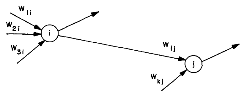
Figure 1: Typical network elements $i$ and $j$ showing connection weights $w$ (reproduced from [30])

Drawing inspiration from biological neurons to implement machine learning was the topic of the first paper presented at the first machine learning conference in 1955 [29, 30] (see Figure 1). It was recognized very early on in the field that direct computational training of neural networks was computationally unfeasible with the computers that were available at that time [35]. The many-fold improvement in neural network computation and theory has made it possible to create neural networks capable of better-than-human performance in a variety of domains [38, 39, 40, 41]. The production of validated data sets [42, 43, 44] and the power of graphic processing units (GPUs) [45, 46, 47, 48] have allowed the effective training of deep neural networks (DNNs) with 100,000s of input features, $N$, and 100s of layers, $L$, that are capable of choosing from among 100,000s categories, $M$ (see Figure 2).

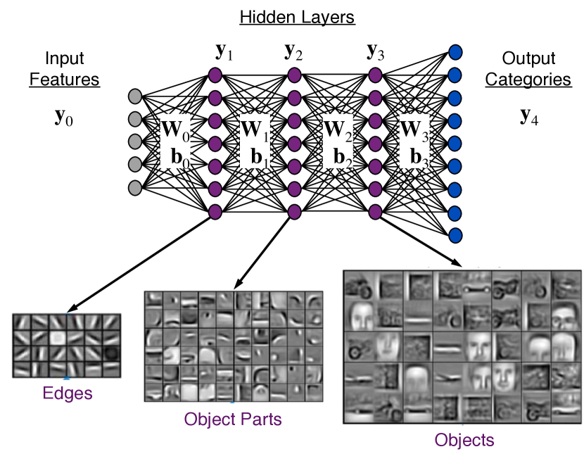
Figure 2: Four layer ($L=4$) deep neural network architecture for categorizing images. The input features ${\bf y}_{0}$ of an image are passed through a series of network layers ${\bf W}_{\ell=0,1,2,3}$, with bias terms ${\bf b}_{\ell=0,1,2,3}$, that produce scores for categories ${\bf y}_{L=4}$. (Figure adapted from [49])

The impressive performance of large DNNs provides motivation to explore even larger networks. However, increasing $N$, $L$, and $M$ each by a factor 10 results in a 1000-fold increase in the memory required for a DNN. Because of these memory constraints, trade-offs are currently being made in terms of precision and accuracy to save storage and computation [50, 51, 52, 11]. Thus, there is significant interest in exploring the effectiveness of sparse DNN representations where many of the weight values are zero. As a comparison, the human brain has approximately 86 billion neurons and 150 trillion synapses [53]. Its graph representation would have approximately 2,000 edges per node, or a density of $2\times 10^{3}/86\times 10^{9}=0.000002\%$.

If a large fraction of the DNN weights can be set to zero, storage and computation costs can be reduced proportionately [6, 54]. The interest in sparse DNNs is not limited to their computational advantages. There has also been extensive theoretical work exploring the potential neuromorphic and algorithmic benefits of sparsity [55, 56, 57, 8, 58].

The primary mathematical operation performed by a DNN network is the inference, or forward propagation, step. Inference is executed repeatedly during training to determine both the weight matrix ${\bf W}_{\ell}$ and the bias vectors ${\bf b}_{\ell}$ of the DNN. The inference computation shown in Figure 2 is given by

$${\bf y}_{\ell+1}=h({\bf y}_{\ell}{\bf W}_{\ell}+{\bf b}_{\ell})$$

where $h()$ is a nonlinear function applied to each element of the vector. The Sparse DNN Challenge uses the standard graph community convention whereby ${\bf W}(i,j)\neq 0$ implies a connection between neuron $i$ and neuron $j$. In this convention ${\bf y}_{\ell}$ are row vectors and left matrix multiply is used to progress through the network. Standard AI definitions can be used by transposing all matrices and multiplying on the right. A commonly used function is the rectified linear unit (ReLU) given by

$$h({\bf y})=\max({\bf y},0)$$

which sets values less that 0 to 0 and leaves other values unchanged. For the Sparse DNN challenge, $h()$ also has an upper limit set to 32. When training a DNN, or performing inference on many different inputs, it is usually necessary to compute multiple ${\bf y}_{\ell}$ vectors at once in a batch that can be denoted as the matrix ${\bf Y}_{\ell}$. In matrix form, the inference step becomes

$${\bf Y}_{\ell+1}=h({\bf Y}_{\ell}{\bf W}_{\ell}+{\bf B}_{\ell})$$

where ${\bf B}_{\ell}$ is a replication of ${\bf b}_{\ell}$ along columns given by

$$\mathbf{B}_{\ell}=\mathbf{b}_{\ell}|\mathbf{Y}_{\ell}\mathbf{1}|_{0}$$

and $\mathbf{1}$ is a column array of 1’s, and $|~{}|_{0}$ is the zero norm.

III Neural Network Data

Scale is an important driver of the Graph Challenge and graphs with billions to trillions of edges are of keen interest. Real sparse neural networks of this size are difficult to obtain from real data. Until such data is available, a reasonable first step is to simulate data with the desired network properties with an emphasis on the difficult part of the problem, in this case: large sparse DNNs.

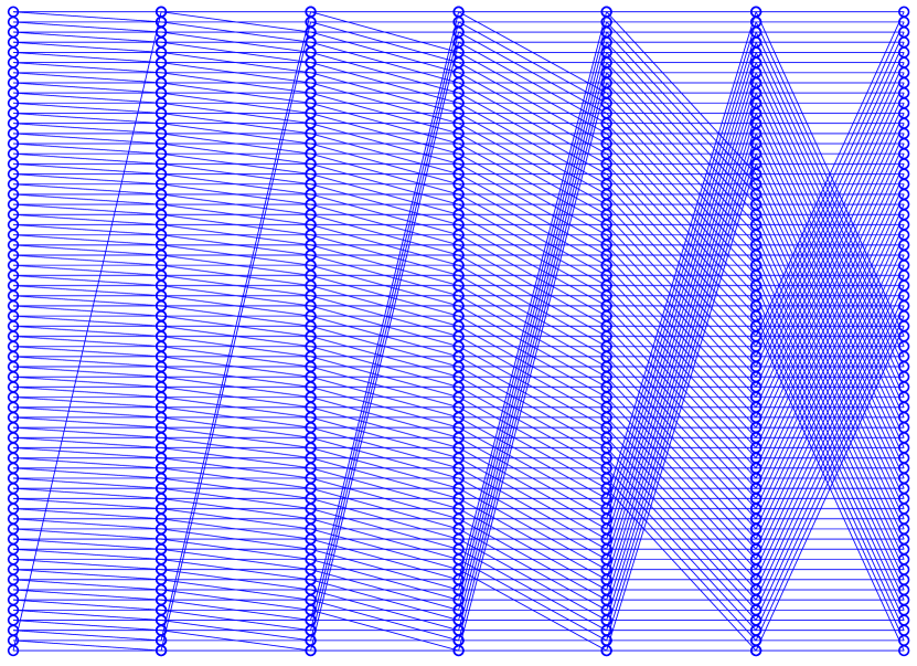
Figure 3: 6 layer, 64 neurons per layer, 2 connections per neuron RadiX-Net DNN produced from Radix set [[2,2,2,2,2,2]]. The Kronecker product of this DNN with [16,16,16,16,16,16,16] produces a 6 layer, 1024 neurons per layer DNN with 32 connections per neuron.

The RadiX-Net synthetic sparse DNN generator is used [59] to efficiently generate a wide range of pre-determined DNNs. RadiX-Net produces DNNs with a number of desirable properties, such as equal number of paths between all inputs, outputs, and intermediate layers. The RadiX-Net DNN generation algorithm uses mixed radices to generate DNNs of specified connectedness (see Figure 3) which are then expanded via Kronecker products into larger DNNs. For the Sparse DNN Challenge different DNNs were created with different numbers of neurons per layer. The RadiX-Net parameters used to create the base DNNs are given in Table I. The base DNNs are then grown to create much deeper DNNs by repeatedly randomly permuting and appending the base DNNs. The permutation process preserves the base DNN properties. The scale of the resulting large sparse DNNs are shown Table II.

Radix Set	Kronecker Set	Layers	Neurons/Layer	Density	Bias
[[2,2,2,2,2,2]]	[16,16,16,16,16,16,16]	6	1024	0.03	-0.30
[[2,2,2,2,2,2,2,2]]	[16,16,16,16,16,16,16,16,16]	8	4096	0.008	-0.35
[[2,2,2,2,2,2,2,2,2,2]]	[16,16,16,16,16,16,16,16,16,16,16]	10	16384	0.002	-0.40
[[2,2,2,2,2,2,2,2,2,2,2,2]]	[16,16,16,16,16,16,16,16,16,16,16,16,16]	12	65536	0.0005	-0.45

Table I: RadiX-Net radix and Kronecker parameters and resulting base DNNs layers, neurons per layer, fraction of non-zeros in weight matrices (density), and bias value. All DNNs have 32 connections per neurons.

	Neurons	Neurons	Neurons	Neurons
Layers	1024	4096	16384	65536
120	3,932,160	15,728,640	62,914,560	251,658,240
480	15,728,640	62,914,560	251,658,240	1,006,632,960
1920	62,914,560	251,658,240	1,006,632,960	4,026,531,840

Table II: Total number of connections = 32x(Layers)x(Neurons) for different large sparse DNNs used in the Sparse DNN Challenge.

IV Input Data Set

Executing the Sparse DNN Challenge requires input data or feature vectors $\mathbf{Y}_{0}$. MNIST (Modified National Institute of Standards and Technology) is a large database of handwritten digits that is widely used for training and testing DNN image processing systems [18]. MNIST consists of 60,000 28$\times$28 pixel images. The Sparse DNN Graph Challenge uses interpolated sparse versions of this entire corpus as input (Figure 5). Each 28$\times$28 pixel image is resized to 32$\times$32 (1024 neurons), 64$\times$64 (4096 neurons), 128$\times$128 (16384 neurons), and 256$\times$256 (65536 neurons). The resized images are thresholded so that all values are either 0 or 1. The images are flattened into a single row to form a feature vector. The non-zero values are written as triples to a .tsv file where each row corresponds to a different image, each column is the non-zero pixel location and the value is 1.

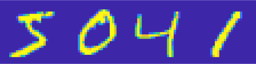
Figure 4: MNIST data set consists of 60,000 handwritten digits [18]. (top) Original 28$\times$28 pixel images of four MNIST images. (bottom) 256$\times$256 resampled thresholded versions of the same images.

V Sparse DNN Challenge

The core the Sparse DNN Challenge is timing DNN inference using the provided DNNs on the provide MNIST input data and verifying the output with provided truth categories. The complete process for performing the challenge consists of the following steps

• Download from GraphChallenge.org: DNN weight matrices $\mathbf{W}_{\ell}$, sparse MNIST input data $\mathbf{Y}_{0}$, and truth categories

• Load a DNN and its corresponding input

• Create and set the appropriate sized bias vectors $\mathbf{b}_{\ell}$ from the table

• Timed: Evaluate the DNN equation for all layers

  $${\bf Y}_{\ell+1}=h({\bf Y}_{\ell}{\bf W}_{\ell}+{\bf B}_{\ell})$$

• Timed: Identify the categories (rows) in final matrix with entries $>0$

• Compare computed categories with truth categories to check correctness

• Compute rate for the DNN: (# inputs) $\times$ (# connections) / time

• Report time and rate for each DNN measured

Reference serial implementations in various programming languages are available at GraphChallenge.org. The Matlab serial reference of the inference calculation is a follows

 

function Y = inferenceReLUvec(W,bias,Y0);

YMAX = 32;

Y = Y0;

for i=1:length(W)

Z = Y*W{i};

b = bias{i};

Y = Z + (double(logical(Z)) .* b);

Y(Y < 0) = 0;

Y(Y > YMAX) = YMAX;

end

end

 

For a given implementation of the Sparse DNN Challenge an implementor should keep the following guidance in mind.

Do

• Use an implementation that could work on real-world data

• Create compressed binary versions of inputs to accelerate reading the data

• Split inputs and run in data parallel mode to achieve higher performance (this requires replicating weight matrices on every processor and can require a lot of memory)

• Split up layers and run in a pipeline parallel mode to achieve higher performance (this saves memory, but requires communicating results after each group of layers)

• Use other reasonable optimizations that would work on real-world data

Avoid

• Exploiting the repetitive structure of weight matrices, weight values, and bias values

• Exploiting layer independence of results

• Using optimizations that would not work on real-world data

VI Computational Metrics

Submissions to the Sparse DNN Challenge will be evaluated on the overall innovations highlighted by the implementation and two metrics: correctness and performance.

VI-A Correctness

Correctness is evaluated by comparing the reported categories with the ground truth categories provided.

VI-B Performance

The performance of the algorithm implementation should be reported in terms of the following metrics:

• Total number of non-zero connections in the given DNN: This measures the amount of data processed

• Execution time: Total time required to perform DNN inference.

• Rate: Measures the throughput of the implementation as the ratio of the number of inputs (e.g., number of MNIST images) times the number of connections in the DNN divided by the execution time.

• Processor: Number and type of processors used in the computation.

VI-C Timing Measurements

Serial timing measurements of the Matlab code are shown in Table III and provide one example for reporting results. Parallel implementations of the Sparse DNN benchmark were developed and tested on the MIT SuperCloud TX-Green supercomputer using pMatlab [60].

Neurons	Layers	Connections	Time	Rate
per Layer		(edges)	(seconds)	(inputs$\times$edges/sec)
1024	120	3,932,160	626	376$\times 10^{6}$
1024	480	15,728,640	2440	386$\times 10^{6}$
1024	1920	62,914,560	9760	386$\times 10^{6}$
4096	120	15,728,640	2446	385$\times 10^{6}$
4096	480	62,914,560	10229	369$\times 10^{6}$
4096	1920	251,658,240	40245	375$\times 10^{6}$
16384	120	62,914,560	10956	344$\times 10^{6}$
16384	480	251,658,240	45268	333$\times 10^{6}$
16384	1920	1,006,632,960	179401	336$\times 10^{6}$
65536	120	251,658,240	45813	329$\times 10^{6}$
65536	480	1,006,632,960	202393	299$\times 10^{6}$
65536	1920	4,026,531,840

Table III: Serial timing measurements of inference rate on different sparse DNNs.

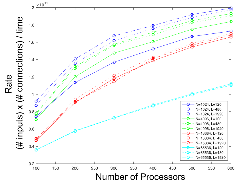
Figure 5: Inference rate versus number of processors for various DNN sizes.

VII Summary

The MIT/IEEE/Amazon GraphChallenge.org encourages community approaches to developing new solutions for analyzing graphs and sparse data. Sparse AI analytics presents unique scalability difficulties. The machine learning, high performance computing, and visual analytics communities have wrestled with these difficulties for decades and developed methodologies for creating challenges to move these communities forward. The proposed Sparse Deep Neural Network (DNN) Challenge draws upon prior challenges from machine learning, high performance computing, and visual analytics to create a challenge that is reflective of emerging sparse AI systems. The Sparse DNN Challenge is a based on a mathematically well-defined DNN inference kernel and can be implemented in any programming environment. Sparse DNN inference is amenable to both vertex-centric implementations and array-based implementations (e.g., using the GraphBLAS.org standard). The computations are simple enough that performance predictions can be made based on simple computing hardware models. The input data sets are derived from the MNIST handwritten letters. The surrounding I/O and verification provide the context for each sparse DNN inference that allows rigorous definition of both the input and the output. Furthermore, since the proposed sparse DNN challenge is scalable in both problem size and hardware, it can be used to measure and quantitatively compare a wide range of present day and future systems. Reference implementations been implemented and their serial and parallel performance have been measured. Specifications, data, and software are publicly available at GraphChallenge.org.

References

- [1] C. Szegedy, Wei Liu, Yangqing Jia, P. Sermanet, S. Reed, D. Anguelov, D. Erhan, V. Vanhoucke, and A. Rabinovich. Going deeper with convolutions. In 2015 IEEE Conference on Computer Vision and Pattern Recognition (CVPR), pages 1–9, June 2015.
- [2] Jeremy Kepner, Vijay Gadepally, Hayden Jananthan, Lauren Milechin, and Sid Samsi. Sparse deep neural network exact solutions. In High Performance Extreme Computing Conference (HPEC). IEEE, 2018.
- [3] Yann LeCun, John S Denker, and Sara A Solla. Optimal brain damage. In Advances in neural information processing systems, pages 598–605, 1990.
- [4] Babak Hassibi and David G Stork. Second order derivatives for network pruning: Optimal brain surgeon. In Advances in neural information processing systems, pages 164–171, 1993.
- [5] Nitish Srivastava, Geoffrey Hinton, Alex Krizhevsky, Ilya Sutskever, and Ruslan Salakhutdinov. Dropout: a simple way to prevent neural networks from overfitting. The Journal of Machine Learning Research, 15(1):1929–1958, 2014.
- [6] Forrest N Iandola, Song Han, Matthew W Moskewicz, Khalid Ashraf, William J Dally, and Kurt Keutzer. Squeezenet: Alexnet-level accuracy with 50x fewer parameters and¡ 0.5 mb model size. arXiv preprint arXiv:1602.07360, 2016.
- [7] Suraj Srinivas and R. Venkatesh Babu. Data-free parameter pruning for deep neural networks. CoRR, abs/1507.06149, 2015.
- [8] Song Han, Huizi Mao, and William J. Dally. Deep compression: Compressing deep neural network with pruning, trained quantization and huffman coding. CoRR, abs/1510.00149, 2015.
- [9] Baoyuan Liu, Min Wang, H. Foroosh, M. Tappen, and M. Penksy. Sparse convolutional neural networks. In 2015 IEEE Conference on Computer Vision and Pattern Recognition (CVPR), pages 806–814, June 2015.
- [10] Jeremy Kepner and John Gilbert. Graph Algorithms in the Language of Linear Algebra. SIAM, 2011.
- [11] Jeremy Kepner, Manoj Kumar, José Moreira, Pratap Pattnaik, Mauricio Serrano, and Henry Tufo. Enabling massive deep neural networks with the graphblas. In High Performance Extreme Computing Conference (HPEC). IEEE, 2017.
- [12] M Kumar, WP Horn, J Kepner, JE Moreira, and P Pattnaik. Ibm power9 and cognitive computing. IBM Journal of Research and Development, 2018.
- [13] J Kepner and H Jananthan. Mathematics of Big Data: Spreadsheets, Databases, Matrices, and Graphs. MIT Press, 2018.
- [14] DARPA. Hierarchical Identify Verify Exploit. https://www.fbo.gov/index?s=opportunity&mode=form&id=e3d5ebb6da9795cd0697cb24293f9302, 2017. [Online; accessed 01-January-2017].
- [15] S. Samsi, V. Gadepally, M. Hurley, M. Jones, E. Kao, S. Mohindra, P. Monticciolo, A. Reuther, S. Smith, W. Song, D. Staheli, and J. Kepner. Static graph challenge: Subgraph isomorphism. In 2017 IEEE High Performance Extreme Computing Conference (HPEC), pages 1–6, Sep. 2017.
- [16] Edward Kao, Vijay Gadepally, Michael Hurley, Michael Jones, Jeremy Kepner, Sanjeev Mohindra, Paul Monticciolo, Albert Reuther, Siddharth Samsi, William Song, Diane Staheli, and Steven Smith. Streaming Graph Challenge - Stochastic Block Partition. Sept 2017.
- [17] J. P. Campbell. Testing with the yoho cd-rom voice verification corpus. In 1995 International Conference on Acoustics, Speech, and Signal Processing, volume 1, pages 341–344 vol.1, May 1995.
- [18] C. Cortes Y. LeCun and C. J.C. Burges. The MNIST Database. http://www.hpcchallenge.org, 2017. [Online; accessed 01-January-2017].
- [19] HPC Challenge. http://yann.lecun.com/exdb/mnist/, 2017. [Online; accessed 01-January-2017].
- [20] Olga Russakovsky, Jia Deng, Hao Su, Jonathan Krause, Sanjeev Satheesh, Sean Ma, Zhiheng Huang, Andrej Karpathy, Aditya Khosla, Michael Bernstein, Alexander C. Berg, and Li Fei-Fei. ImageNet Large Scale Visual Recognition Challenge. International Journal of Computer Vision (IJCV), 115(3):211–252, 2015.
- [21] Kristin A. Cook, Georges Grinstein, and Mark A. Whiting. The VAST Challenge: History, Scope, and Outcomes: An introduction to the Special Issue. Information Visualization, 13(4):301-312, Oct 2014.
- [22] Jean Scholtz, Mark A. Whiting, Catherine Plaisant, and Georges Grinstein. A Reflection on Seven Years of the VAST Challenge. In Proceedings of the 2012 BELIV Workshop: Beyond Time and Errors - Novel Evaluation Methods for Visualization, BELIV ’12, pages 13:1–13:8. ACM, 2012.
- [23] D Bader, Kamesh Madduri, John Gilbert, Viral Shah, Jeremy Kepner, Theresa Meuse, and Ashok Krishnamurthy. Designing scalable synthetic compact applications for benchmarking high productivity computing systems. Cyberinfrastructure Technology Watch, 2:1–10, 2006.
- [24] Jurij Leskovec, Deepayan Chakrabarti, Jon Kleinberg, and Christos Faloutsos. Realistic, mathematically tractable graph generation and evolution, using kronecker multiplication. In European Conference on Principles of Data Mining and Knowledge Discovery, pages 133–145. Springer, 2005.
- [25] Patrick Dreher, Chansup Byun, Chris Hill, Vijay Gadepally, Bradley Kuszmaul, and Jeremy Kepner. Pagerank pipeline benchmark: Proposal for a holistic system benchmark for big-data platforms. In Parallel and Distributed Processing Symposium Workshops, 2016 IEEE International, pages 929–937. IEEE, 2016.
- [26] Mauro Bisson, Everett Phillips, and Massimiliano Fatica. A cuda implementation of the pagerank pipeline benchmark. In High Performance Extreme Computing Conference (HPEC), 2016 IEEE, pages 1–7. IEEE, 2016.
- [27] M. M. Wolf, J. W. Berry, and D. T. Stark. A task-based linear algebra building blocks approach for scalable graph analytics. In 2015 IEEE High Performance Extreme Computing Conference (HPEC), pages 1–6, Sept 2015.
- [28] M. M. Wolf, H. C. Edwards, and S. L. Olivier. Kokkos/qthreads task-parallel approach to linear algebra based graph analytics. In 2016 IEEE High Performance Extreme Computing Conference (HPEC), pages 1–7, Sept 2016.
- [29] Willis H Ware. Introduction to session on learning machines. In Proceedings of the March 1-3, 1955, western joint computer conference, pages 85–85. ACM, 1955.
- [30] WESLEY A Clark and Bernard G Farley. Generalization of pattern recognition in a self-organizing system. In Proceedings of the March 1-3, 1955, western joint computer conference, pages 86–91. ACM, 1955.
- [31] Oliver G Selfridge. Pattern recognition and modern computers. In Proceedings of the March 1-3, 1955, western joint computer conference, pages 91–93. ACM, 1955.
- [32] GP Dinneen. Programming pattern recognition. In Proceedings of the March 1-3, 1955, western joint computer conference, pages 94–100. ACM, 1955.
- [33] Allen Newell. The chess machine: an example of dealing with a complex task by adaptation. In Proceedings of the March 1-3, 1955, western joint computer conference, pages 101–108. ACM, 1955.
- [34] John McCarthy, Marvin L Minsky, Nathaniel Rochester, and Claude E Shannon. A proposal for the dartmouth summer research project on artificial intelligence, august 31, 1955. AI magazine, 27(4):12, 2006.
- [35] Marvin Minsky and Oliver G Selfridge. Learning in random nets. In Information theory : papers read at a symposium on information theory held at the Royal Institution, London, August 29th to September 2nd, pages 335–347. Butterworths, London, 1960.
- [36] Marvin Minsky. Steps toward artificial intelligence. Proceedings of the IRE, 49(1):8–30, 1961.
- [37] Arthur L Samuel. Some studies in machine learning using the game of checkers. IBM Journal of research and development, 3(3):210–229, 1959.
- [38] Richard Lippmann. An introduction to computing with neural nets. IEEE Assp magazine, 4(2):4–22, 1987.
- [39] Douglas A Reynolds, Thomas F Quatieri, and Robert B Dunn. Speaker verification using adapted gaussian mixture models. Digital signal processing, 10(1-3):19–41, 2000.
- [40] Alex Krizhevsky, Ilya Sutskever, and Geoffrey E Hinton. Imagenet classification with deep convolutional neural networks. In Advances in neural information processing systems, pages 1097–1105, 2012.
- [41] Yann LeCun, Yoshua Bengio, and Geoffrey Hinton. Deep learning. Nature, 521(7553):436–444, 2015.
- [42] Joseph P Campbell. Testing with the yoho cd-rom voice verification corpus. In Acoustics, Speech, and Signal Processing, 1995. ICASSP-95., 1995 International Conference on, volume 1, pages 341–344. IEEE, 1995.
- [43] Yann LeCun, Corinna Cortes, and Christopher JC Burges. The mnist database of handwritten digits, 1998.
- [44] Jia Deng, Wei Dong, Richard Socher, Li-Jia Li, Kai Li, and Li Fei-Fei. Imagenet: A large-scale hierarchical image database. In Computer Vision and Pattern Recognition, 2009. CVPR 2009. IEEE Conference on, pages 248–255. IEEE, 2009.
- [45] Murray Campbell, A Joseph Hoane, and Feng-hsiung Hsu. Deep blue. Artificial intelligence, 134(1-2):57–83, 2002.
- [46] Michael P McGraw-Herdeg, Douglas P Enright, and B Scott Michel. Benchmarking the nvidia 8800gtx with the cuda development platform. HPEC 2007 Proceedings, 2007.
- [47] Andrew Kerr, Dan Campbell, and Mark Richards. Gpu performance assessment with the hpec challenge. In HPEC Workshop 2008, 2008.
- [48] Edward A Epstein, Marshall I Schor, BS Iyer, Adam Lally, Eric W Brown, and Jaroslaw Cwiklik. Making watson fast. IBM Journal of Research and Development, 56(3.4):15–1, 2012.
- [49] Honglak Lee, Roger Grosse, Rajesh Ranganath, and Andrew Y Ng. Convolutional deep belief networks for scalable unsupervised learning of hierarchical representations. In Proceedings of the 26th annual international conference on machine learning, pages 609–616. ACM, 2009.
- [50] Baoyuan Liu, Min Wang, Hassan Foroosh, Marshall Tappen, and Marianna Pensky. Sparse convolutional neural networks. In Proceedings of the IEEE Conference on Computer Vision and Pattern Recognition, pages 806–814, 2015.
- [51] Andrew Lavin and Scott Gray. Fast algorithms for convolutional neural networks. In Proceedings of the IEEE Conference on Computer Vision and Pattern Recognition, pages 4013–4021, 2016.
- [52] Norman P Jouppi, Cliff Young, Nishant Patil, David Patterson, Gaurav Agrawal, Raminder Bajwa, Sarah Bates, Suresh Bhatia, Nan Boden, Al Borchers, et al. In-datacenter performance analysis of a tensor processing unit. arXiv preprint arXiv:1704.04760, 2017.
- [53] Frederico A.C. Azevedo, Ludmila R.B. Carvalho, Lea T. Grinberg, Jos Marcelo Farfel, Renata E.L. Ferretti, Renata E.P. Leite, Wilson Jacob Filho, Roberto Lent, and Suzana Herculano-Houzel. Equal numbers of neuronal and nonneuronal cells make the human brain an isometrically scaled-up primate brain. The Journal of Comparative Neurology, 513(5):532–541, 2009.
- [54] Shaohuai Shi and Xiaowen Chu. Speeding up convolutional neural networks by exploiting the sparsity of rectifier units. arXiv preprint arXiv:1704.07724, 2017.
- [55] Honglak Lee, Chaitanya Ekanadham, and Andrew Y Ng. Sparse deep belief net model for visual area v2. In Advances in neural information processing systems, pages 873–880, 2008.
- [56] Marc’aurelio Ranzato, Y-lan Boureau, and Yann L Cun. Sparse feature learning for deep belief networks. In Advances in neural information processing systems, pages 1185–1192, 2008.
- [57] Xavier Glorot, Antoine Bordes, and Yoshua Bengio. Deep sparse rectifier neural networks. In Aistats, volume 15, page 275, 2011.
- [58] Dong Yu, Frank Seide, Gang Li, and Li Deng. Exploiting sparseness in deep neural networks for large vocabulary speech recognition. In Acoustics, Speech and Signal Processing (ICASSP), 2012 IEEE International Conference on, pages 4409–4412. IEEE, 2012.
- [59] Ryan Robinett and Jeremy Kepner. Radix-net: Structured sparse matrices for deep neural networks. In Proceedings of the 2015 IEEE International Parallel and Distributed Processing Symposium Workshop, IPDPSW ’19. IEEE Computer Society, 2019.
- [60] Jeremy Kepner. Parallel MATLAB for Multicore and Multinode Computers. SIAM, 2009.