ā€ ā€ thanks: astrid.ordell@thep.lu.seā€ ā€ thanks: roman.pasechnik@thep.lu.seā€ ā€ thanks: hugo.serodio@thep.lu.se

Classification of anomaly-free 2HDMs with a gauged Uā€‹(1)ā€²š‘ˆsuperscript1ā€²U(1)^{\prime} symmetry

Franz Nottensteiner Department of Astronomy and Theoretical Physics, Lund University, SE-223 62 Lund, Sweden ā€ƒā€ƒ Astrid Ordell Department of Astronomy and Theoretical Physics, Lund University, SE-223 62 Lund, Sweden ā€ƒā€ƒ Roman Pasechnik Department of Astronomy and Theoretical Physics, Lund University, SE-223 62 Lund, Sweden ā€ƒā€ƒ Hugo SerĆ“dio Department of Astronomy and Theoretical Physics, Lund University, SE-223 62 Lund, Sweden
(March 19, 2024)
Abstract

Two-Higgs-doublet models (2HDMs) with a flavored Uā€‹(1)ā€²š‘ˆsuperscript1ā€²U(1)^{\prime} gauge symmetry are a popular extension to the Standard Model (SM), yet they currently lack a complete survey. In this paper, we present a full classification of anomaly-free 2HDMs within the SM fermion content, resulting in a total of eleven distinct models. Four of these are relatively well-studied, while the rest either partially, or entirely, lack previous treatment. We study these textures under a variety of experimental bounds, focusing mainly on the previously unexplored models. This work is intended to act as a catalog to models worth considering in greater detail.

ā€ ā€ preprint: LU TP 19-42

I Introduction

With the discovery of the Higgs bosonĀ AadĀ etĀ al. (2012a); ChatrchyanĀ etĀ al. (2012), the Standard Model (SM) has reinforced itself as the most accurate description of high-energy physics. While the SM has endured all kinds of experimental scrutiny, it still leaves room for sizable new physics (NP) effects. For the past decades, many extensions have been proposed. One of the most popular SM extensions is the two-Higgs-doublet model (2HDM)Ā BrancoĀ etĀ al. (2012); Ivanov (2017), where a single additional copy of the Higgs doublet is added to the SM. Such a simple scenario introduces, nevertheless, new types of interactions; a general 2HDM implementation is plagued by tree-level flavor-changing neutral currents (FCNCs) mediated by the new scalarsĀ CrivellinĀ etĀ al. (2013). To circumvent such a problem, the Yukawa textures are constrained with various additional symmetries. In the so-called natural flavor-conserving 2HDM implementations, an additional ā„¤2subscriptā„¤2\mathbb{Z}_{2} is added, leading to the complete absence of tree-level FCNCsĀ GlashowĀ andĀ Weinberg (1977); Paschos (1977). Larger symmetries can also be introduced, and a popular scenario is the one known as the Branco-Grimus-Lavoura (BGL) modelĀ BrancoĀ etĀ al. (1996), where a ā„¤nā‰„3subscriptā„¤š‘›3\mathbb{Z}_{n\geq 3} symmetry is used. In the BGL, there are FCNCs present at tree level; however, due to the specific symmetry implementation, they turn out to be highly suppressed Ć  la minimal flavor violationĀ BurasĀ etĀ al. (2001); Dā€™AmbrosioĀ etĀ al. (2002).

A complete survey of 2HDMs with an Abelian flavor symmetry, either discrete or continuous, has been done by Ferreira and SilvaĀ FerreiraĀ andĀ Silva (2011) (later confirmed through different methods in Refs.Ā SerĆ“dio (2013); IvanovĀ andĀ Nishi (2013)). From the initially available 318superscript3183^{18} model implementations, and under the imposition of physical constraints in the quark sector, the authors were able to reduce this number down to 246246246 model candidates. In the vast majority of these implementations, the symmetry group is either the Uā€‹(1)š‘ˆ1U(1) or a ā„¤nā‰„3subscriptā„¤š‘›3\mathbb{Z}_{n\geq 3}, which from the scalar potential point of view is not distinguishable and will always lead to the presence of an accidental Goldstone bosonĀ IvanovĀ etĀ al. (2012). Since many of these implementations use the global version of the symmetry, a common practice is to softly break it in the scalar potential. Another way is to promote the symmetry to a local one, turning the extra Goldstone boson into the longitudinal component of the new gauge field, i.e.Ā the Zā€²superscriptš‘ā€²Z^{\prime} boson. Some of the pioneering work on anomaly-free 2HDMs with a gauged Abelian symmetry can be found in Refs.Ā DavidsonĀ etĀ al. (1979a, b); DavidsonĀ andĀ Wali (1980).

In the present work, we look into the general classification and phenomenology of flavored Uā€‹(1)ā€²š‘ˆsuperscript1ā€²U(1)^{\prime} gauge symmetries in the context of 2HDMs. This was initiated as a master thesis project, and some of the details on the procedure can be found in Ref.Ā Teichmann (2017).111Note that the authorā€™s family name has been changed from Teichmann to Nottensteiner. We find that, out of the 246246246, only 111111 distinct models survive anomaly cancellation. Out of this small subset, five of the models can be found in the literature with partial or complete phenomenological studies. The remaining scenarios were virtually unexplored until now. All these findings assumed only the SM fermionic content. Neutrinos can get their mass by a large number of different mechanisms and, therefore, deserve a detailed study on their own.

The paper is organized as follows: In Sec.Ā II, we introduce the framework, notation and the general procedure used for the classification. Section III contains a detailed implementation of all 11 viable models, while, in Sec.Ā IV, we present an analysis of phenomenological constraints of the new models. The results in this section serve as a first step in the phenomenological validation of such models with relatively light NP fields. We conclude and summarize our findings in Sec.Ā VI. Additional details on the scalar potential and the anomaly conditions can be found in the Appendixes.

II Abelian Flavor symmetries in 2HDMs

II.1 2HDM Yukawa sector

In this work, we consider a 2HDM with an additional gauged Uā€‹(1)ā€²š‘ˆsuperscript1ā€²U(1)^{\prime} symmetry. There is always at least one Higgs doublet charged under Uā€‹(1)ā€²š‘ˆsuperscript1ā€²U(1)^{\prime}; however, if the only scale entering into its spontaneous breaking is the electroweak (EW) scale, it becomes extensively challenging to accommodate a relatively heavy Zā€²superscriptš‘ā€²Z^{\prime} gauge boson without deviating from the SM Zš‘Z currents.222Scenarios where the Zā€²superscriptš‘ā€²Z^{\prime} are exceedingly light, due to a very small gauge coupling, can be an alternative. However, in the models presented here, the meson observables would anyway place very strong constraints on such scenarios (see Sec.Ā IV). We do not further explore this option. The particle content, in the scalar sector, is thus enlarged by an additional scalar singlet Sš‘†S, charged under the new Abelian symmetry.

We parameterize the scalar fields as

Ī¦a=12ā€‹(2ā€‹Ļ•a+vaā€‹eiā€‹Ī±a+Ra+iā€‹Ia),S=12ā€‹(vSā€‹eiā€‹Ī±S+Ļ+iā€‹Ī·),formulae-sequencesubscriptĪ¦š‘Ž12matrix2subscriptsuperscriptitalic-Ļ•š‘Žsubscriptš‘£š‘Žsuperscriptš‘’š‘–subscriptš›¼š‘Žsubscriptš‘…š‘Žš‘–subscriptš¼š‘Žš‘†12subscriptš‘£š‘†superscriptš‘’š‘–subscriptš›¼š‘†šœŒš‘–šœ‚\displaystyle\begin{split}\Phi_{a}&=\frac{1}{\sqrt{2}}\begin{pmatrix}\sqrt{2}\phi^{+}_{a}\\ v_{a}\,e^{i\alpha_{a}}+R_{a}+iI_{a}\end{pmatrix}\,,\\[2.27621pt] S&=\frac{1}{\sqrt{2}}\left(v_{S}\,e^{i\alpha_{S}}+\rho+i\eta\right)\,,\end{split} (1)

with a=1,2š‘Ž12a=1,2, va,Ssubscriptš‘£š‘Žš‘†v_{a,S} the vacuum expectation values (VEVs) of the scalar fields and v12+v22=vā‰ƒ246ā€‹GeVsuperscriptsubscriptš‘£12superscriptsubscriptš‘£22š‘£similar-to-or-equals246GeV\sqrt{v_{1}^{2}+v_{2}^{2}}=v\simeq 246\,\text{GeV}. The presence of two Abelian symmetries allows us to rephase the scalar fields such that Ī±1=Ī±2=0subscriptš›¼1subscriptš›¼20\alpha_{1}=\alpha_{2}=0 and Ī±Sā‰ 0subscriptš›¼š‘†0\alpha_{S}\neq 0 can be chosen without the loss of generality. This choice for the phases will be used throughout this paper. Note that the inclusion of the scalar singlet, even though essential for phenomenological tests, does not effect the model classification. For details on the scalar potential, see Appendix A.

The Yukawa interactions for quarks and charged leptons are, in the flavor basis, given by

āˆ’ā„’Yukawa=qL0ĀÆā€‹Ī“aā€‹Ī¦aā€‹dR0+qL0ĀÆā€‹Ī”aā€‹Ī¦~aā€‹uR0+ā„“L0ĀÆā€‹Ī aā€‹Ī¦aā€‹eR0+H.c.,formulae-sequencesubscriptā„’YukawaĀÆsuperscriptsubscriptš‘žL0subscriptĪ“š‘ŽsubscriptĪ¦š‘Žsubscriptsuperscriptš‘‘0RĀÆsuperscriptsubscriptš‘žL0subscriptĪ”š‘Žsubscript~Ī¦š‘Žsubscriptsuperscriptš‘¢0RĀÆsuperscriptsubscriptā„“L0subscriptĪ š‘ŽsubscriptĪ¦š‘Žsubscriptsuperscriptš‘’0RHc\displaystyle\begin{split}-\mathcal{L}_{\mathrm{Yukawa}}&=\overline{q_{\mathrm{L}}^{0}}\,\Gamma_{a}\Phi_{a}\,d^{0}_{\mathrm{R}}+\overline{q_{\mathrm{L}}^{0}}\,\Delta_{a}\tilde{\Phi}_{a}\,u^{0}_{\mathrm{R}}\\ &+\overline{\ell_{\mathrm{L}}^{0}}\,\Pi_{a}\Phi_{a}\,e^{0}_{\mathrm{R}}+\mathrm{H.c.}\,,\end{split} (2)

with Ī¦~a=iā€‹Ļƒ2ā€‹Ī¦aāˆ—subscript~Ī¦š‘Žš‘–subscriptšœŽ2superscriptsubscriptĪ¦š‘Ž\tilde{\Phi}_{a}=i\sigma_{2}{\Phi}_{a}^{*}, where Ļƒ2subscriptšœŽ2\sigma_{2} is the Pauli matrix. As stated in the introduction, the fermionic content is the SM one with the fields defined in the generic flavor basis. After EW symmetry breaking, the mass matrices take the form

Mu=12ā€‹(v1ā€‹Ī”1+v2ā€‹Ī”2),Md=12ā€‹(v1ā€‹Ī“1+v2ā€‹Ī“2),Me=12ā€‹(v1ā€‹Ī 1+v2ā€‹Ī 2).formulae-sequencesubscriptš‘€š‘¢12subscriptš‘£1subscriptĪ”1subscriptš‘£2subscriptĪ”2formulae-sequencesubscriptš‘€š‘‘12subscriptš‘£1subscriptĪ“1subscriptš‘£2subscriptĪ“2subscriptš‘€š‘’12subscriptš‘£1subscriptĪ 1subscriptš‘£2subscriptĪ 2\displaystyle\begin{split}M_{u}&=\frac{1}{\sqrt{2}}\left(v_{1}\Delta_{1}+v_{2}\Delta_{2}\right)\,,\\ M_{d}&=\frac{1}{\sqrt{2}}\left(v_{1}\Gamma_{1}+v_{2}\Gamma_{2}\right)\,,\\ M_{e}&=\frac{1}{\sqrt{2}}\left(v_{1}\Pi_{1}+v_{2}\Pi_{2}\right)\,.\end{split} (3)

These matrices are then diagonalized via the unitary field transformations fLā€‹(R)0=ULā€‹(R)ā€‹fLā€‹(R)subscriptsuperscriptš‘“0LRsubscriptš‘ˆLRsubscriptš‘“LRf^{0}_{\mathrm{L(R)}}=U_{\mathrm{L(R)}}f_{\mathrm{L(R)}}, such that

UfLā€ ā€‹Mfā€‹UfR=Dfwithf={u,d,e},formulae-sequencesuperscriptsubscriptš‘ˆfLā€ subscriptš‘€š‘“subscriptš‘ˆfRsubscriptš·š‘“withš‘“š‘¢š‘‘š‘’\displaystyle U_{\mathrm{fL}}^{\dagger}M_{f}U_{\mathrm{fR}}=D_{f}\quad\text{with}\quad f=\{u,d,e\}\,, (4)

where Dfsubscriptš·š‘“D_{f} is a diagonal matrix with the ordered masses.

In the 2HDM there is a unique orthogonal combination, per fermionic sector, that can be defined and that carries all the information about flavor-changing iterations in the mass eigenbasis, namely,

Nu=12ā€‹UuLā€ ā€‹(v2ā€‹Ī”1āˆ’v1ā€‹Ī”2)ā€‹UuR,Nd=12ā€‹UdLā€ ā€‹(v2ā€‹Ī“1āˆ’v1ā€‹Ī“2)ā€‹UdR,Ne=12ā€‹UeLā€ ā€‹(v2ā€‹Ī 1āˆ’v1ā€‹Ī 2)ā€‹UeR.formulae-sequencesubscriptš‘š‘¢12superscriptsubscriptš‘ˆuLā€ subscriptš‘£2subscriptĪ”1subscriptš‘£1subscriptĪ”2subscriptš‘ˆuRformulae-sequencesubscriptš‘š‘‘12superscriptsubscriptš‘ˆdLā€ subscriptš‘£2subscriptĪ“1subscriptš‘£1subscriptĪ“2subscriptš‘ˆdRsubscriptš‘š‘’12superscriptsubscriptš‘ˆeLā€ subscriptš‘£2subscriptĪ 1subscriptš‘£1subscriptĪ 2subscriptš‘ˆeR\displaystyle\begin{split}N_{u}&=\frac{1}{\sqrt{2}}U_{\mathrm{uL}}^{\dagger}\left(v_{2}\Delta_{1}-v_{1}\Delta_{2}\right)U_{\mathrm{uR}}\,,\\ N_{d}&=\frac{1}{\sqrt{2}}U_{\mathrm{dL}}^{\dagger}\left(v_{2}\Gamma_{1}-v_{1}\Gamma_{2}\right)U_{\mathrm{dR}}\,,\\ N_{e}&=\frac{1}{\sqrt{2}}U_{\mathrm{eL}}^{\dagger}\left(v_{2}\Pi_{1}-v_{1}\Pi_{2}\right)U_{\mathrm{eR}}\,.\end{split} (5)

Any off-diagonal component in Eq.Ā (5) can be further emphasized by presenting it in the following form

Nu=tĪ²ā€‹Duāˆ’(tĪ²+tĪ²āˆ’1)ā€‹v22ā€‹UuLā€ ā€‹Ī”2ā€‹UuR,Nd=tĪ²ā€‹Ddāˆ’(tĪ²+tĪ²āˆ’1)ā€‹v22ā€‹UdLā€ ā€‹Ī“2ā€‹UdR,Ne=tĪ²ā€‹Deāˆ’(tĪ²+tĪ²āˆ’1)ā€‹v22ā€‹UeLā€ ā€‹Ī 2ā€‹UeR,formulae-sequencesubscriptš‘š‘¢subscriptš‘”š›½subscriptš·š‘¢subscriptš‘”š›½superscriptsubscriptš‘”š›½1subscriptš‘£22superscriptsubscriptš‘ˆuLā€ subscriptĪ”2subscriptš‘ˆuRformulae-sequencesubscriptš‘š‘‘subscriptš‘”š›½subscriptš·š‘‘subscriptš‘”š›½superscriptsubscriptš‘”š›½1subscriptš‘£22superscriptsubscriptš‘ˆdLā€ subscriptĪ“2subscriptš‘ˆdRsubscriptš‘š‘’subscriptš‘”š›½subscriptš·š‘’subscriptš‘”š›½superscriptsubscriptš‘”š›½1subscriptš‘£22superscriptsubscriptš‘ˆeLā€ subscriptĪ 2subscriptš‘ˆeR\displaystyle\begin{split}N_{u}&={t}_{\beta}D_{u}-\left({t}_{\beta}+{t}_{\beta}^{-1}\right)\frac{v_{2}}{\sqrt{2}}\;U_{\mathrm{uL}}^{\dagger}\Delta_{2}U_{\mathrm{uR}}\,,\\ N_{d}&={t}_{\beta}D_{d}-\left({t}_{\beta}+{t}_{\beta}^{-1}\right)\frac{v_{2}}{\sqrt{2}}\;U_{\mathrm{dL}}^{\dagger}\Gamma_{2}U_{\mathrm{dR}}\,,\\ N_{e}&={t}_{\beta}D_{e}-\left({t}_{\beta}+{t}_{\beta}^{-1}\right)\frac{v_{2}}{\sqrt{2}}\;U_{\mathrm{eL}}^{\dagger}\Pi_{2}U_{\mathrm{eR}}\,,\end{split} (6)

with tĪ²ā‰”tanā”Ī²=v2/v1subscriptš‘”š›½š›½subscriptš‘£2subscriptš‘£1{t}_{\beta}\equiv\tan\beta=v_{2}/v_{1}, and where the latter term can be expressed in terms of projectors on the quark mass matrices. For further convenience, we can single out the sources of tree-level FCNCs mediated by scalar fields into the dimensionless quantities

š’¦u=UuLā€ ā€‹Ī”2ā€‹UuR,š’¦d=UdLā€ ā€‹Ī“2ā€‹UdR,š’¦e=UeLā€ ā€‹Ī 2ā€‹UeR.\displaystyle\begin{split}\mathcal{K}_{u}=&U_{\mathrm{uL}}^{\dagger}\Delta_{2}U_{\mathrm{uR}}\,,\quad\mathcal{K}_{d}=U_{\mathrm{dL}}^{\dagger}\Gamma_{2}U_{\mathrm{dR}}\,,\\ \mathcal{K}_{e}=&U_{\mathrm{eL}}^{\dagger}\Pi_{2}U_{\mathrm{eR}}\,.\end{split} (7)

The specific form for these quantities is texture dependent and will be specified for all models in Sec.Ā III.

II.2 The new gauge sector

In this section, we introduce the relevant interactions of the new gauge field, in addition to discussing the role played by the scalar singlet. Under the corresponding Abelian symmetry, the field transformations are given by

qL0jā†’eiā€‹Ī±ā€‹Xqjā€‹qL0j,dR0jā†’eiā€‹Ī±ā€‹Xdjā€‹dR0j,uR0jā†’eiā€‹Ī±ā€‹Xujā€‹uR0j,ā„“L0jā†’eiā€‹Ī±ā€‹Xā„“jā€‹ā„“L0j,eR0jā†’eiā€‹Ī±ā€‹Xejā€‹eR0jĪ¦aā†’eiā€‹Ī±ā€‹XĪ¦aā€‹Ī¦a,Sā†’eiā€‹Ī±ā€‹XSā€‹S.formulae-sequenceformulae-sequenceā†’subscriptsuperscriptsubscriptš‘žL0š‘—superscriptš‘’š‘–š›¼subscriptš‘‹subscriptš‘žš‘—subscriptsuperscriptsubscriptš‘žL0š‘—formulae-sequenceā†’subscriptsuperscriptsubscriptš‘‘R0š‘—superscriptš‘’š‘–š›¼subscriptš‘‹subscriptš‘‘š‘—subscriptsuperscriptsubscriptš‘‘R0š‘—formulae-sequenceā†’subscriptsuperscriptsubscriptš‘¢R0š‘—superscriptš‘’š‘–š›¼subscriptš‘‹subscriptš‘¢š‘—subscriptsuperscriptsubscriptš‘¢R0š‘—formulae-sequenceā†’subscriptsuperscriptsubscriptā„“L0š‘—superscriptš‘’š‘–š›¼subscriptš‘‹subscriptā„“š‘—subscriptsuperscriptsubscriptā„“L0š‘—ā†’subscriptsuperscriptsubscriptš‘’R0š‘—superscriptš‘’š‘–š›¼subscriptš‘‹subscriptš‘’š‘—subscriptsuperscriptsubscriptš‘’R0š‘—subscriptĪ¦š‘Žā†’superscriptš‘’š‘–š›¼subscriptš‘‹subscriptĪ¦š‘ŽsubscriptĪ¦š‘Žā†’š‘†superscriptš‘’š‘–š›¼subscriptš‘‹š‘†š‘†\displaystyle\begin{split}&{q_{\mathrm{L}}^{0}}_{j}\rightarrow e^{i\alpha X_{q_{j}}}{q_{\mathrm{L}}^{0}}_{j},\;{d_{\mathrm{R}}^{0}}_{j}\rightarrow e^{i\alpha X_{d_{j}}}{d_{\mathrm{R}}^{0}}_{j},\;{u_{\mathrm{R}}^{0}}_{j}\rightarrow e^{i\alpha X_{u_{j}}}{u_{\mathrm{R}}^{0}}_{j},\\ &{\ell_{\mathrm{L}}^{0}}_{j}\rightarrow e^{i\alpha X_{\ell_{j}}}{\ell_{\mathrm{L}}^{0}}_{j},\;\;{e_{\mathrm{R}}^{0}}_{j}\rightarrow e^{i\alpha X_{e_{j}}}{e_{\mathrm{R}}^{0}}_{j}\\ &\Phi_{a}\rightarrow e^{i\alpha X_{\Phi_{a}}}\Phi_{a},\;S\rightarrow e^{i\alpha X_{S}}S\,.\end{split} (8)

The charges of the fields are, in general, flavor dependent and denoted by the label of the corresponding field. We will, throughout the paper, use a compact matrix notation for the charges. For example, for qLsubscriptš‘žLq_{\mathrm{L}},

š’³qā‰”diagā€‹(Xq1,Xq2,Xq3),superscriptš’³š‘ždiagsubscriptš‘‹subscriptš‘ž1subscriptš‘‹subscriptš‘ž2subscriptš‘‹subscriptš‘ž3\displaystyle\mathcal{X}^{q}\equiv\text{diag}(X_{q_{1}},X_{q_{2}},X_{q_{3}})\,, (9)

and similarly for all the other fields.

A convenient basis to write the relevant Lagrangian for the gauge sector is the would-be SM basis, i.e. the mass eigenbasis for the Zš‘Z gauge boson in the absence of mixing with the new Zā€²superscriptš‘ā€²Z^{\prime} boson. In such a basis, the fields and free parameters carry a hat. The neutral gauge interactions after EW symmetry breaking are then given by

ā„’Zā€²=āˆ’14ā€‹Z^Ī¼ā€‹Ī½ā€‹Z^Ī¼ā€‹Ī½āˆ’14ā€‹Z^Ī¼ā€‹Ī½ā€²ā€‹Z^ā€²ā£Ī¼ā€‹Ī½+12ā€‹M^Z2ā€‹Z^Ī¼ā€‹Z^Ī¼+12ā€‹M^Zā€²2ā€‹Z^Ī¼ā€²ā€‹Z^ā€²ā£Ī¼+Ī“ā€‹M^ZZā€²2ā€‹Z^Ī¼ā€‹Z^ā€²ā£Ī¼āˆ’Z^Ī¼(ā€²)ā€‹ĻˆĀÆā€‹Ī³Ī¼ā€‹Q^Z(ā€²)Ļˆā€‹Ļˆāˆ’Z^Ī¼(ā€²)ā€‹(āˆ‚Ī¼Ļ•ā€ ā€‹Q^Z(ā€²)Ļ•ā€‹Ļ•āˆ’Ļ•ā€ ā€‹Q^Z(ā€²)Ļ•ā€‹āˆ‚Ī¼Ļ•),subscriptā„’superscriptZā€²14subscript^š‘šœ‡šœˆsuperscript^š‘šœ‡šœˆ14subscriptsuperscript^š‘ā€²šœ‡šœˆsuperscript^š‘ā€²šœ‡šœˆ12superscriptsubscript^š‘€Z2subscript^š‘šœ‡superscript^š‘šœ‡12superscriptsubscript^š‘€superscriptZā€²2subscriptsuperscript^š‘ā€²šœ‡superscript^š‘ā€²šœ‡š›æsuperscriptsubscript^š‘€superscriptZZā€²2subscript^š‘šœ‡superscript^š‘ā€²šœ‡subscriptsuperscript^š‘ā€²šœ‡ĀÆšœ“superscriptš›¾šœ‡superscriptsubscript^š‘„superscriptZā€²šœ“šœ“subscriptsuperscript^š‘ā€²šœ‡subscriptšœ‡superscriptitalic-Ļ•ā€ superscriptsubscript^š‘„superscriptZā€²italic-Ļ•italic-Ļ•superscriptitalic-Ļ•ā€ superscriptsubscript^š‘„superscriptZā€²italic-Ļ•subscriptšœ‡italic-Ļ•\displaystyle\begin{split}\mathcal{L}_{\mathrm{Z^{\prime}}}=&-\frac{1}{4}\hat{Z}_{\mu\nu}\hat{Z}^{\mu\nu}-\frac{1}{4}\hat{Z}^{\prime}_{\mu\nu}\hat{Z}^{\prime\mu\nu}\\ &+\frac{1}{2}\hat{M}_{\mathrm{Z}}^{2}\hat{Z}_{\mu}\hat{Z}^{\mu}+\frac{1}{2}\hat{M}_{\mathrm{Z^{\prime}}}^{2}\hat{Z}^{\prime}_{\mu}\hat{Z}^{\prime\mu}+\delta\hat{M}_{\mathrm{ZZ^{\prime}}}^{2}\hat{Z}_{\mu}\hat{Z}^{\prime\mu}\\ &-\hat{Z}^{(\prime)}_{\mu}\,\overline{\psi}\,\gamma^{\mu}\hat{Q}_{\mathrm{Z^{(\prime)}}}^{\psi}\,\psi\\ &-\hat{Z}^{(\prime)}_{\mu}\left(\partial_{\mu}\phi^{\dagger}\,\hat{Q}_{\mathrm{Z^{(\prime)}}}^{\phi}\,\phi-\phi^{\dagger}\,\hat{Q}_{\mathrm{Z^{(\prime)}}}^{\phi}\,\partial_{\mu}\phi\right)\,,\end{split} (10)

in addition to all quartic interactions, where Ļˆ={uL/R0,dL/R0,eL/R0,Ī½L0}šœ“subscriptsuperscriptš‘¢0LRsubscriptsuperscriptš‘‘0LRsubscriptsuperscriptš‘’0LRsubscriptsuperscriptšœˆ0L\psi=\{u^{0}_{\mathrm{L/R}},d^{0}_{\mathrm{L/R}},e^{0}_{\mathrm{L/R}},\nu^{0}_{\mathrm{L}}\} and Ļ•={Ļ•a+,Ra,Ia,Ļ,Ī·}italic-Ļ•superscriptsubscriptitalic-Ļ•š‘Žsubscriptš‘…š‘Žsubscriptš¼š‘ŽšœŒšœ‚\phi=\{\phi_{a}^{+},R_{a},I_{a},\rho,\eta\} and where we assume the gauge kinetic mixing to be zero.

The first and second line of Eq.Ā (10) includes the mass terms for the Z^āˆ’Z^ā€²^š‘superscript^š‘ā€²\hat{Z}-\hat{Z}^{\prime} system, which in the would-be SM basis are explicitly given by

M^Z2=14ā€‹f^2ā€‹v2,M^Zā€²2=gā€²ā£2ā€‹(va2ā€‹XĪ¦a2+vS2ā€‹XS2),Ī“ā€‹M^ZZā€²2=āˆ’12ā€‹f^ā€‹gā€²ā€‹(va2ā€‹XĪ¦a),\displaystyle\begin{split}\hat{M}_{\mathrm{Z}}^{2}=&\frac{1}{4}\hat{f}^{2}v^{2}\,,\quad\hat{M}_{\mathrm{Z^{\prime}}}^{2}=g^{\prime 2}\left(v_{a}^{2}X_{\Phi_{a}}^{2}+v_{S}^{2}X_{S}^{2}\right)\,,\\ \delta\hat{M}_{\mathrm{{Z}{Z}^{\prime}}}^{2}=&-\frac{1}{2}\hat{f}g^{\prime}\left(v_{a}^{2}X_{\Phi_{a}}\right)\,,\end{split} (11)

with f^=e^/sĪøā€‹cĪø^š‘“^š‘’subscriptš‘ šœƒsubscriptš‘šœƒ\hat{f}=\hat{e}/s_{\theta}c_{\theta}, where e^^š‘’\hat{e} is the electromagnetic charge in the would-be SM basis. In the absence of mass mixing, i.e. Ī“ā€‹M^2=0š›æsuperscript^š‘€20\delta\hat{M}^{2}=0, the gauge boson Z^^š‘\hat{Z} is identified with the SM Zš‘Z boson and we can lose the hat notation. We would then have the MSĀÆĀÆMS\overline{\text{MS}} weak mixing angle sĪø2ā‰ƒ0.231157ā€‹(23)similar-to-or-equalssuperscriptsubscriptš‘ šœƒ20.23115723s_{\theta}^{2}\simeq 0.231157(23), while the on-shell weak mixing angle, extracted by Ī½ā€‹Nšœˆš‘\nu N experimentsĀ TanabashiĀ etĀ al. (2018), is given by sW2ā‰”1āˆ’mW2/mZ2=sĪø2āˆ’ā€EW-loopā€ā‰ƒ0.2237ā€‹(9)superscriptsubscriptš‘ š‘Š21superscriptsubscriptš‘šš‘Š2superscriptsubscriptš‘šš‘2superscriptsubscriptš‘ šœƒ2ā€EW-loopā€similar-to-or-equals0.22379s_{W}^{2}\equiv 1-m_{W}^{2}/m_{Z}^{2}=s_{\theta}^{2}-\text{"EW-loop"}\simeq 0.2237(9). For a nonzero mass mixing, the value of sĪøsubscriptš‘ šœƒs_{\theta} gets modifiedĀ BabuĀ etĀ al. (1998) (see Sec.Ā IV for more details).

In the most general scenario, the mixing between Z^^š‘\hat{Z} and Z^ā€²superscript^š‘ā€²\hat{Z}^{\prime} is removed through the orthogonal field transformation

(Z^Ī¼Z^Ī¼ā€²)=(cMsMāˆ’sMcM)ā€‹(ZĪ¼ZĪ¼ā€²),sMā‰”sinā”(ĪøM),formulae-sequencematrixsubscript^š‘šœ‡subscriptsuperscript^š‘ā€²šœ‡matrixsubscriptš‘š‘€subscriptš‘ š‘€subscriptš‘ š‘€subscriptš‘š‘€matrixsubscriptš‘šœ‡subscriptsuperscriptš‘ā€²šœ‡subscriptš‘ š‘€subscriptšœƒš‘€\displaystyle\begin{pmatrix}\hat{Z}_{\mu}\\ \hat{Z}^{\prime}_{\mu}\end{pmatrix}=\begin{pmatrix}c_{M}&s_{M}\\ -s_{M}&c_{M}\end{pmatrix}\begin{pmatrix}Z_{\mu}\\ Z^{\prime}_{\mu}\end{pmatrix}\,,\quad s_{M}\equiv\sin(\theta_{M})\,, (12)

with

tanā”(2ā€‹ĪøM)=2ā€‹Ī“ā€‹M^ZZā€²2M^Zā€²2āˆ’M^Z2,2subscriptšœƒš‘€2š›æsuperscriptsubscript^š‘€superscriptZZā€²2superscriptsubscript^š‘€superscriptZā€²2superscriptsubscript^š‘€Z2\displaystyle\tan(2\theta_{M})=\frac{2\delta\hat{M}_{\mathrm{ZZ^{\prime}}}^{2}}{\hat{M}_{\mathrm{Z^{\prime}}}^{2}-\hat{M}_{\mathrm{Z}}^{2}}\,, (13)

such that, in the mass eigenbasis for the gauge fields, the masses of Zš‘Z and Zā€²superscriptš‘ā€²Z^{\prime} are given by

mZ(ā€²)2=M^Z(ā€²)2āˆ’(+)tMā€‹Ī“ā€‹M^Zā€‹Zā€²2.superscriptsubscriptš‘šsuperscriptš‘ā€²2fragments()superscriptsubscript^š‘€superscriptš‘ā€²2subscriptš‘”š‘€š›æsubscriptsuperscript^š‘€2š‘superscriptš‘ā€²\displaystyle\begin{split}m_{Z^{(\prime)}}^{2}&=\hat{M}_{Z^{(\prime)}}^{2}\mathbin{\vbox{\hbox{\oalign{\hfil$\scriptstyle-$\hfil\cr\kern-2.15277pt\cr$\scriptscriptstyle({+})$\cr}}}}t_{M}\delta\hat{M}^{2}_{ZZ^{\prime}}\,.\end{split} (14)

In the final two lines of Eq.Ā (10) we have interactions between the massive neutral gauge bosons and the fermionic and bosonic matter, respectively. The couplings are matrices in flavor space, explicitly given by

Q^Zi=f^ā€‹(T3iāˆ’sĪø2ā€‹Qi),Q^Zā€²i=gā€²ā€‹š’³i,\displaystyle\begin{split}\hat{Q}_{\mathrm{Z}}^{i}&=\hat{f}(T^{i}_{3}-s_{\theta}^{2}Q^{i})\,,\quad\hat{Q}_{\mathrm{Z^{\prime}}}^{i}=g^{\prime}\mathcal{X}^{i}\,,\end{split} (15)

with i=uL,R,dL,R,ā„“L,eLš‘–subscriptš‘¢LRsubscriptš‘‘LRsubscriptā„“Lsubscriptš‘’Li=u_{\mathrm{L,R}},\;d_{\mathrm{L,R}},\;\ell_{\mathrm{L}},\;e_{\mathrm{L}}. In the mass eigenbasis for the gauge fields, we then have that

QZi=cMā€‹Q^Ziāˆ’sMā€‹Q^Zā€²i,QZā€²i=sMā€‹Q^Zi+cMā€‹Q^Zā€²i,\displaystyle\begin{split}Q_{\mathrm{Z}}^{i}=&c_{M}\hat{Q}_{\mathrm{Z}}^{i}-s_{M}\hat{Q}_{\mathrm{Z^{\prime}}}^{i}\,,\quad Q_{\mathrm{Z^{\prime}}}^{i}=s_{M}\hat{Q}_{\mathrm{Z}}^{i}+c_{M}\hat{Q}_{\mathrm{Z^{\prime}}}^{i}\,,\end{split} (16)

where T3subscriptš‘‡3T_{3} is the isospin and Qš‘„Q the electric charge, and with Qā‰”T3+Yš‘„subscriptš‘‡3š‘ŒQ\equiv T_{3}+Y, where Yš‘ŒY is the hypercharge.

Note that, in the mass eigenbasis for the matter fields, Q^Zisuperscriptsubscript^š‘„Zš‘–\hat{Q}_{\mathrm{Z}}^{i} retain its form, while Q^Zā€²isuperscriptsubscript^š‘„superscriptZā€²š‘–\hat{Q}_{\mathrm{Z^{\prime}}}^{i} acquires a generic flavor structure, i.e.

Q^Zā€²iāŸ¶Q^Zā€²i=gā€²ā€‹Uiā€ ā€‹š’³iā€‹Uiā‰”gā€²ā€‹Īži.āŸ¶superscriptsubscript^š‘„superscriptZā€²š‘–superscriptsubscript^š‘„superscriptZā€²š‘–superscriptš‘”ā€²superscriptsubscriptš‘ˆš‘–ā€ superscriptš’³š‘–subscriptš‘ˆš‘–superscriptš‘”ā€²subscriptĪžš‘–\displaystyle\begin{split}\hat{Q}_{\mathrm{Z^{\prime}}}^{i}\longrightarrow\hat{Q}_{\mathrm{Z^{\prime}}}^{i}=g^{\prime}U_{i}^{\dagger}\mathcal{X}^{i}U_{i}\equiv g^{\prime}\Xi_{i}.\end{split} (17)

In accordance with the scalar sector, all sources of tree-level FCNCs mediated by the neutral gauge bosons, are encoded in the dimensionless quantity ĪžisubscriptĪžš‘–\Xi_{i}. Further details on the specific form of these couplings are given for all models in Sec.Ā III.

II.3 General procedure for anomaly-free solutions

In 2011, Ferreira and Silva classified all possible implementations of a global Abelian symmetry in the quark sector of a 2HDM FerreiraĀ andĀ Silva (2011). In short, they used that a flavored symmetry transformation, such as the one defined in Eq.Ā (8), imposes constraints on the Yukawa couplings. In order for the Yukawa Lagrangian, in Eq.Ā (2), to remain invariant under such field transformations, the following constraints have to be fulfilled (for the quark sector)

(Ī“a)iā€‹j=eiā€‹Īøā€‹(Xqiāˆ’Xdjāˆ’XĪ¦a)ā€‹(Ī“a)iā€‹j,(Ī”a)iā€‹j=eiā€‹Īøā€‹(Xqiāˆ’Xuj+XĪ¦a)ā€‹(Ī”a)iā€‹j,formulae-sequencesubscriptsubscriptĪ“š‘Žš‘–š‘—superscriptš‘’š‘–šœƒsubscriptš‘‹subscriptš‘žš‘–subscriptš‘‹subscriptš‘‘š‘—subscriptš‘‹subscriptĪ¦š‘ŽsubscriptsubscriptĪ“š‘Žš‘–š‘—subscriptsubscriptĪ”š‘Žš‘–š‘—superscriptš‘’š‘–šœƒsubscriptš‘‹subscriptš‘žš‘–subscriptš‘‹subscriptš‘¢š‘—subscriptš‘‹subscriptĪ¦š‘ŽsubscriptsubscriptĪ”š‘Žš‘–š‘—\displaystyle\begin{split}(\Gamma_{a})_{ij}&=e^{i\theta(X_{q_{i}}-X_{d_{j}}-X_{\Phi_{a}})}(\Gamma_{a})_{ij}\,,\\ (\Delta_{a})_{ij}&=e^{i\theta(X_{q_{i}}-X_{u_{j}}+X_{\Phi_{a}})}(\Delta_{a})_{ij}\,,\end{split} (18)

such that

(Ī“a)iā€‹j=anyifā€‹Xqiāˆ’Xdj=XĪ¦a,(Ī“a)iā€‹j=0ifā€‹Xqiāˆ’Xdjā‰ XĪ¦a,formulae-sequencesubscriptsubscriptĪ“š‘Žš‘–š‘—anyformulae-sequenceifsubscriptš‘‹subscriptš‘žš‘–subscriptš‘‹subscriptš‘‘š‘—subscriptš‘‹subscriptĪ¦š‘Žformulae-sequencesubscriptsubscriptĪ“š‘Žš‘–š‘—0ifsubscriptš‘‹subscriptš‘žš‘–subscriptš‘‹subscriptš‘‘š‘—subscriptš‘‹subscriptĪ¦š‘Ž\displaystyle\begin{split}(\Gamma_{a})_{ij}&=\mathrm{any\;\;\;\;if}\;\;X_{q_{i}}-X_{d_{j}}=X_{\Phi_{a}}\,,\\ (\Gamma_{a})_{ij}&=0\;\;\;\;\;\;\;\;\mathrm{if}\;\;X_{q_{i}}-X_{d_{j}}\neq X_{\Phi_{a}}\,,\end{split} (19)

and similarly for the up sector, with a=1,2š‘Ž12a=1,2, j=1,2,3š‘—123j=1,2,3, and with no summation over repeated indices.333The case of a possible discrete Abelian symmetry was also tackled inĀ FerreiraĀ andĀ Silva (2011). However, those cases are of no relevance in our study. On top of these constraints, one can add three extra physical requirements:

  • (i)

    no massless up-type quarks, i.e.Ā detā€‹Muā‰ 0detsubscriptš‘€š‘¢0\text{det}\hskip 1.42262ptM_{u}\neq 0ā€†;

  • (ii)

    no massless down-type quarks, i.e.Ā detā€‹Mdā‰ 0detsubscriptš‘€š‘‘0\text{det}\hskip 1.42262ptM_{d}\neq 0ā€†;

  • (iii)

    possibility for Dirac-type Cā€‹Pš¶š‘ƒCP violation at tree level, i.e.Ā detā€‹[Muā€‹Muā€ ,Mdā€‹Mdā€ ]ā‰ 0detsubscriptš‘€š‘¢superscriptsubscriptš‘€š‘¢ā€ subscriptš‘€š‘‘superscriptsubscriptš‘€š‘‘ā€ 0\text{det}[M_{u}M_{u}^{\dagger},M_{d}M_{d}^{\dagger}]\neq 0ā€†.

In Ref.Ā FerreiraĀ andĀ Silva (2011), a weaker formulation of (iii) was used, demanding the Cabibbo-Kobayashi-Maskawa (CKM) mixing matrix to be non-block diagonal.444For the models obtained, there is no real difference between the two formulations, but the latter has a more straightforward implementation when dealing with generic textures. From these simple requirements, in addition to excluding any models equivalent up to permutations,555Any transformation that preserves the flavor symmetry, i.e. any simultaneous permutation of rows or independent permutation of columns, will result in an equivalent model. The row (column) permutations simply alter the constraints in such a way that the corresponding left (right) charges are exchanged, resulting in the procedure merely amounting to a relabelling of flavor indices. the number of viable texture combinations was reduced down from 318superscript3183^{18} to 246246246.

In contrast to Ferreira and Silva, we now wish to classify all possible implementations of a gauged Abelian symmetry in the 2HDM, in addition to including not only the SM quarks but also the SM charged leptons. With the Abelian symmetry now being gauged, we must also make sure that the solutions are anomaly-free. The six anomaly conditions which do not cancel trivially are presented in Appendix B and involve

[Sā€‹Uā€‹(2)L]2ā€‹Uā€‹(1)ā€²,[Sā€‹Uā€‹(3)C]2ā€‹Uā€‹(1)ā€²,[Uā€‹(1)Y]2ā€‹Uā€‹(1)ā€²,Uā€‹(1)Yā€‹[Uā€‹(1)ā€²]2,[Uā€‹(1)ā€²]3,[Gravity]2ā€‹Uā€‹(1)ā€².superscriptdelimited-[]š‘†š‘ˆsubscript2L2š‘ˆsuperscript1ā€²superscriptdelimited-[]š‘†š‘ˆsubscript3C2š‘ˆsuperscript1ā€²superscriptdelimited-[]š‘ˆsubscript1Y2š‘ˆsuperscript1ā€²š‘ˆsubscript1Ysuperscriptdelimited-[]š‘ˆsuperscript1ā€²2superscriptdelimited-[]š‘ˆsuperscript1ā€²3superscriptdelimited-[]Gravity2š‘ˆsuperscript1ā€²\displaystyle\begin{split}&[{SU}(2)_{\mathrm{L}}]^{2}{U}(1)^{\prime},\;\;\;[{SU}(3)_{\mathrm{C}}]^{2}{U}(1)^{\prime},\\ &[{U}(1)_{\mathrm{Y}}]^{2}{U}(1)^{\prime},\;\;\;{U}(1)_{\mathrm{Y}}[{U}(1)^{\prime}]^{2},\\ &[{U}(1)^{\prime}]^{3},\;\;\;[\mathrm{Gravity}]^{2}{U}(1)^{\prime}\,.\end{split} (20)

There has been plenty of activity over the past decades on finding efficient ways of extracting generic solutions of such a system of equationsĀ BatraĀ etĀ al. (2006); AllanachĀ etĀ al. (2019); RathsmanĀ andĀ Tellander (2019); CostaĀ etĀ al. (2019).666There are different approaches where the anomaly constraints can be relaxed. The so-called Green-Schwarz mechanismĀ GreenĀ andĀ Schwarz (1984, 1985); GreenĀ etĀ al. (1985) or effective anomalous Uā€‹(1)ā€²š‘ˆsuperscript1ā€²U(1)^{\prime} scenariosĀ Preskill (1991); CorianoĀ etĀ al. (2007); IrgesĀ etĀ al. (2008); EkstedtĀ etĀ al. (2018), are some of the popular ones. We shall not pursue this line further and consider only models that cancel all the anomaly equations.

To find all valid models, we use, as a starting point, the subset of textures in Ref.Ā FerreiraĀ andĀ Silva (2011) corresponding to a continuous symmetry. The textures are then, in correspondence with the anomaly conditions, converted into constraints for the charges just like in Eq.Ā (19). When including the charged leptons, there is no need to perform the whole procedure in Ref.Ā FerreiraĀ andĀ Silva (2011) once more, as the lepton textures are highly constrained by the anomaly equations. Instead, we need only to impose the additional physical requirement

  • (iv)

    no massless charged leptons, i.e. detā€‹Meā‰ 0detsubscriptš‘€š‘’0\text{det}\hskip 1.42262ptM_{e}\neq 0.

For a 2HDM, this additional requirement can be fulfilled only when the combined texture of Ī 1subscriptĪ 1\Pi_{1} and Ī 2subscriptĪ 2\Pi_{2} have at least one nonzero entry in each row and each column. There are, hence, six possible minimal combined textures, but, since they are all equivalent up to permutations, it is of interest to consider only one of them, e.g.Ā the diagonal one

(I)Ī 1:(ƗƗƗ)ā€‹Ī 2:(),(II)Ī 1:(ƗƗ)ā€‹Ī 2:(Ɨ),(III)Ī 1:(Ɨ)ā€‹Ī 2:(ƗƗ),(IV)Ī 1:()ā€‹Ī 2:(ƗƗƗ),:IsubscriptĪ 1matrixmissing-subexpressionmissing-subexpressionmissing-subexpressionmissing-subexpressionmissing-subexpressionmissing-subexpressionsubscriptĪ 2:matrixmissing-subexpressionmissing-subexpressionmissing-subexpressionmissing-subexpressionmissing-subexpressionmissing-subexpressionIIsubscriptĪ 1:matrixmissing-subexpressionmissing-subexpressionmissing-subexpressionmissing-subexpressionsubscriptĪ 2:matrixmissing-subexpressionmissing-subexpressionmissing-subexpressionmissing-subexpressionmissing-subexpressionmissing-subexpressionmissing-subexpressionmissing-subexpressionIIIsubscriptĪ 1:matrixmissing-subexpressionmissing-subexpressionmissing-subexpressionmissing-subexpressionmissing-subexpressionsubscriptĪ 2:matrixmissing-subexpressionmissing-subexpressionmissing-subexpressionmissing-subexpressionmissing-subexpressionmissing-subexpressionmissing-subexpressionIVsubscriptĪ 1:matrixmissing-subexpressionmissing-subexpressionmissing-subexpressionmissing-subexpressionmissing-subexpressionmissing-subexpressionsubscriptĪ 2:matrixmissing-subexpressionmissing-subexpressionmissing-subexpressionmissing-subexpressionmissing-subexpressionmissing-subexpression\displaystyle\begin{split}(\mathrm{I})&\;\;\;\;\;\Pi_{1}:\begin{pmatrix}\times&\makebox[0.0pt][c]{}&\makebox[0.0pt][c]{}\\ \makebox[0.0pt][c]{}&\times&\makebox[0.0pt][c]{}\\ \makebox[0.0pt][c]{}&\makebox[0.0pt][c]{}&\times\end{pmatrix}\hskip 8.53581pt\Pi_{2}:\begin{pmatrix}\makebox[0.0pt][c]{}&\makebox[0.0pt][c]{}&\makebox[0.0pt][c]{}\\ \makebox[0.0pt][c]{}&\makebox[0.0pt][c]{}&\makebox[0.0pt][c]{}\\ \makebox[0.0pt][c]{}&\makebox[0.0pt][c]{}&\makebox[0.0pt][c]{}\end{pmatrix},\\ (\mathrm{II})&\;\;\;\;\;\Pi_{1}:\begin{pmatrix}\times&\makebox[0.0pt][c]{}&\makebox[0.0pt][c]{}\\ \makebox[0.0pt][c]{}&\times&\makebox[0.0pt][c]{}\\ \makebox[0.0pt][c]{}&\makebox[0.0pt][c]{}&\makebox[0.0pt][c]{}\end{pmatrix}\hskip 8.53581pt\Pi_{2}:\begin{pmatrix}\makebox[0.0pt][c]{}&\makebox[0.0pt][c]{}&\makebox[0.0pt][c]{}\\ \makebox[0.0pt][c]{}&\makebox[0.0pt][c]{}&\makebox[0.0pt][c]{}\\ \makebox[0.0pt][c]{}&\makebox[0.0pt][c]{}&\times\end{pmatrix},\\ (\mathrm{III})&\;\;\;\;\;\Pi_{1}:\begin{pmatrix}\times&\makebox[0.0pt][c]{}&\makebox[0.0pt][c]{}\\ \makebox[0.0pt][c]{}&\makebox[0.0pt][c]{}&\makebox[0.0pt][c]{}\\ \makebox[0.0pt][c]{}&\makebox[0.0pt][c]{}&\makebox[0.0pt][c]{}\end{pmatrix}\hskip 8.53581pt\Pi_{2}:\begin{pmatrix}\makebox[0.0pt][c]{}&\makebox[0.0pt][c]{}&\makebox[0.0pt][c]{}\\ \makebox[0.0pt][c]{}&\times&\makebox[0.0pt][c]{}\\ \makebox[0.0pt][c]{}&\makebox[0.0pt][c]{}&\times\end{pmatrix},\\ (\mathrm{IV})&\;\;\;\;\;\Pi_{1}:\begin{pmatrix}\makebox[0.0pt][c]{}&\makebox[0.0pt][c]{}&\makebox[0.0pt][c]{}\\ \makebox[0.0pt][c]{}&\makebox[0.0pt][c]{}&\makebox[0.0pt][c]{}\\ \makebox[0.0pt][c]{}&\makebox[0.0pt][c]{}&\makebox[0.0pt][c]{}\end{pmatrix}\hskip 8.53581pt\Pi_{2}:\begin{pmatrix}\times&\makebox[0.0pt][c]{}&\makebox[0.0pt][c]{}\\ \makebox[0.0pt][c]{}&\times&\makebox[0.0pt][c]{}\\ \makebox[0.0pt][c]{}&\makebox[0.0pt][c]{}&\times\end{pmatrix},\end{split} (21)

corresponding to the constraints

  • (I)

    Xā„“iāˆ’Xei=XĪ¦1subscriptš‘‹subscriptā„“š‘–subscriptš‘‹subscriptš‘’š‘–subscriptš‘‹subscriptĪ¦1\;\;X_{\ell_{i}}-X_{e_{i}}=X_{\Phi_{1}}ā€†,

  • (II)

    Xā„“1ā€‹(2)āˆ’Xe1ā€‹(2)=XĪ¦1subscriptš‘‹subscriptā„“12subscriptš‘‹subscriptš‘’12subscriptš‘‹subscriptĪ¦1\;\;X_{\ell_{1(2)}}-X_{e_{1(2)}}=X_{\Phi_{1}}ā€ƒand ā€ƒXā„“3āˆ’Xe3=XĪ¦2subscriptš‘‹subscriptā„“3subscriptš‘‹subscriptš‘’3subscriptš‘‹subscriptĪ¦2X_{\ell_{3}}-X_{e_{3}}=X_{\Phi_{2}}ā€†,

  • (III)

    Xā„“1āˆ’Xe1=XĪ¦1subscriptš‘‹subscriptā„“1subscriptš‘‹subscriptš‘’1subscriptš‘‹subscriptĪ¦1\;\;X_{\ell_{1}}-X_{e_{1}}=X_{\Phi_{1}}ā€ƒand ā€ƒXā„“2ā€‹(3)āˆ’Xe2ā€‹(3)=XĪ¦2subscriptš‘‹subscriptā„“23subscriptš‘‹subscriptš‘’23subscriptš‘‹subscriptĪ¦2X_{\ell_{2(3)}}-X_{e_{2(3)}}=X_{\Phi_{2}}ā€†,

  • (IV)

    Xā„“iāˆ’Xei=XĪ¦2subscriptš‘‹subscriptā„“š‘–subscriptš‘‹subscriptš‘’š‘–subscriptš‘‹subscriptĪ¦2\;\;X_{\ell_{i}}-X_{e_{i}}=X_{\Phi_{2}}ā€†.

Note that these conditions are sufficient for generating any allowed lepton texture, and not just the minimal ones in (I)āˆ’(IV)IIV(\mathrm{I})-(\mathrm{IV}), as constraints on the form Xā„“iāˆ’Xejā‰ XĪ¦asubscriptš‘‹subscriptā„“š‘–subscriptš‘‹subscriptš‘’š‘—subscriptš‘‹subscriptĪ¦š‘ŽX_{\ell_{i}}-X_{e_{j}}\neq X_{\Phi_{a}} are not included. In our case, however, the textures in (I)āˆ’(IV)IIV(\mathrm{I})-(\mathrm{IV}) are, in fact, the only ones allowed, as the anomaly conditions are highly constraining. The only exception to this is a special case of the models presented in Sec.Ā III.1, for which all leptons, and the Higgs doublet that they couple to, have zero Uā€‹(1)ā€²š‘ˆsuperscript1ā€²U(1)^{\prime} charge. For such a scenario, the leptons are free to have any texture, provided that the physical condition in (iv)iv(\mathrm{iv}) is still fulfilled.

If a solution exists where all constraints are met, while simultaneously all charges are rational numbers and the quarks textures are not destroyed, the model is labeled as valid.777For an explicit example of a valid and invalid model, seeĀ Teichmann (2017) Out of the 246 models in Ref.Ā FerreiraĀ andĀ Silva (2011), there are 116 of them corresponding to continuous symmetries, out of which only 11 nondegenerate models survive these constraints. Here, we emphasize that we do not scan to find viable solutions; we loop over every possible combination of constraints and solve the system for each instance. As such, we are guaranteed to find all solutions.

To identify degenerate solutions, we consider all possible permutations of the textures, i.e.Ā every possible combination of i,j,kš‘–š‘—š‘˜i,j,k for the transformation

Ī“1,2ā€²=š’«iTā€‹Ī“1,2ā€‹š’«j,Ī”1,2ā€²=š’«iTā€‹Ī”1,2ā€‹š’«k,formulae-sequencesubscriptsuperscriptĪ“ā€²12superscriptsubscriptš’«š‘–TsubscriptĪ“12subscriptš’«š‘—subscriptsuperscriptĪ”ā€²12superscriptsubscriptš’«š‘–TsubscriptĪ”12subscriptš’«š‘˜\Gamma^{\prime}_{1,2}=\mathcal{P}_{i}^{\mathrm{T}}\Gamma_{1,2}\mathcal{P}_{j},\;\;\Delta^{\prime}_{1,2}=\mathcal{P}_{i}^{\mathrm{T}}\Delta_{1,2}\mathcal{P}_{k}, (22)

where š’«š’«\mathcal{P} is the three-dimensional representation of the permutation group S3subscriptš‘†3S_{3}, such that i,j,kš‘–š‘—š‘˜i,j,k ranges from one to six. The permutations on the left are shared by both quark sectors, while the permutations on the right are independent. With this corresponding to an ordered sampling with replacement, there is a total of 63=216superscript632166^{3}=216 possible permutations for each model.

III Anomaly-Free Models

Up to permutations, there are a total of seven valid models. Four of these come in two editions, aš‘Ža and bš‘b, where bš‘b has the flipped texture with respect to aš‘Ža, i.e. Ī“1ā†”Ī”2ā†”subscriptĪ“1subscriptĪ”2\Gamma_{1}\leftrightarrow\Delta_{2}, Ī“2ā†”Ī”1ā†”subscriptĪ“2subscriptĪ”1\Gamma_{2}\leftrightarrow\Delta_{1}. For each model, we present the allowed textures and some analytical predictions, with the corresponding charges specified in Table 2. An overview on which of the models that have been studied previously, in either its global or gauged form, can be found in Table 1.

As a first validity check for the less-studied models, this section includes a parameter scan for fitting the quark masses and mixings (MMs). The best-fit points then serve as input values when accounting for all the remaining observables in Sec.Ā IV.

For all models, except M5 and M6, the free parameters in the Yukawa sector are

  • ā€¢

    Yukawa couplings modulus āˆˆ[10āˆ’5,5]absentsuperscript1055\in[10^{-5},5];

  • ā€¢

    Yukawa couplings argument āˆˆ[10āˆ’10,2Ļ€[\in[10^{-10},2\pi[;

  • ā€¢

    doublet fields VEVs, i.e. tanā”Ī²āˆˆ[10āˆ’3,103]š›½superscript103superscript103\tan\beta\in[10^{-3},10^{3}].

The scan was performed by giving, as input, 300 different tanā”Ī²š›½\tan\beta values evenly distributed in logarithmic scale. For the models M5 and M6, on the other hand, it is more convenient to parameterize the Yukawa couplings with the physical quark masses and CKM mixing angles (see the respective model subsection for the explicit parameterization). For the fermions masses and CKM mixing matrix data, we have used Ref.Ā TanabashiĀ etĀ al. (2018). The charged lepton mass matrix is diagonal in all models and, therefore, the extraction of their Yukawa couplings is straightforward.

Model Global Uā€‹(1)ā€²š‘ˆsuperscript1ā€²U(1)^{\prime} Gauged Uā€‹(1)ā€²š‘ˆsuperscript1ā€²U(1)^{\prime}
M1 GlashowĀ andĀ Weinberg (1977); HaberĀ etĀ al. (1979) CrivellinĀ etĀ al. (2015a); CamargoĀ etĀ al. (2019a); CamposĀ etĀ al. (2017); CamargoĀ etĀ al. (2019b)
M2 - -
M3a,ā€†b - CelisĀ etĀ al. (2017); CrivellinĀ etĀ al. (2015b); BianĀ etĀ al. (2018, 2017); KoĀ etĀ al. (2019)
M4a,ā€†b - -
M5 AlvesĀ etĀ al. (2018) NomuraĀ andĀ Okada (2017)
M6a,ā€†b BrancoĀ etĀ al. (1996); BotellaĀ etĀ al. (2014) CelisĀ etĀ al. (2015)
M7a,ā€†b - -
Table 1: An overview of the valid models, where previous studies are indicated by the corresponding reference.

III.1 Leptons that couple exclusively to one Higgs

In this section, we present all models fulfilling the constraints specified in Sec.Ā II.3, while simultaneously having the leptons coupling to only one of the Higgs doublets. In all these models, there exists a particular charge assignment for which one of the scalar doublets, as well as all charged leptons, is uncharged under Uā€‹(1)ā€²š‘ˆsuperscript1ā€²U(1)^{\prime}. In this special case, all models can fulfill the anomaly constraints even without the introduction of charged leptons.

III.1.1 Model M1

Let us begin with the one model that is naturally flavor conserving, namely,

Ī“1:(ƗƗƗƗƗƗƗƗƗ)Ī“2:(000000000)Ī”1:(ƗƗƗƗƗƗƗƗƗ)Ī”2:(000000000),:subscriptĪ“1matrixsubscriptĪ“2:matrix000000000subscriptĪ”1:matrixsubscriptĪ”2:matrix000000000\displaystyle\begin{split}\Gamma_{1}&:\begin{pmatrix}\times&\times&\times\\ \times&\times&\times\\ \times&\times&\times\end{pmatrix}\hskip 5.69054pt\Gamma_{2}:\begin{pmatrix}\makebox[0.0pt][c]{0}&\makebox[0.0pt][c]{0}&\makebox[0.0pt][c]{0}\\ \makebox[0.0pt][c]{0}&\makebox[0.0pt][c]{0}&\makebox[0.0pt][c]{0}\\ \makebox[0.0pt][c]{0}&\makebox[0.0pt][c]{0}&\makebox[0.0pt][c]{0}\end{pmatrix}\hskip 5.69054pt\\ \Delta_{1}&:\begin{pmatrix}\times&\times&\times\\ \times&\times&\times\\ \times&\times&\times\end{pmatrix}\hskip 4.2679pt\Delta_{2}:\begin{pmatrix}\makebox[0.0pt][c]{0}&\makebox[0.0pt][c]{0}&\makebox[0.0pt][c]{0}\\ \makebox[0.0pt][c]{0}&\makebox[0.0pt][c]{0}&\makebox[0.0pt][c]{0}\\ \makebox[0.0pt][c]{0}&\makebox[0.0pt][c]{0}&\makebox[0.0pt][c]{0}\end{pmatrix},\end{split} (23)

with the corresponding charges specified in Table 2. As is familiar, this model has no tree-level FCNCs, since š’¦d,u=0subscriptš’¦š‘‘š‘¢0\mathcal{K}_{d,u}=0 and ĪžisubscriptĪžš‘–\Xi_{i} are diagonal.

For the particular choice of y=3ā€‹xš‘¦3š‘„y=3x, the Uā€‹(1)ā€²š‘ˆsuperscript1ā€²U(1)^{\prime} symmetry places no constraints on the Yukawa quark textures, and we instead end up with the most general 2HDM. This trivially allowed texture is not considered further in this work.

Model XqLsubscriptš‘‹subscriptš‘žšæX_{q_{L}} XuRsubscriptš‘‹subscriptš‘¢š‘…X_{u_{R}} XdRsubscriptš‘‹subscriptš‘‘š‘…X_{d_{R}} Xā„“Lsubscriptš‘‹subscriptā„“šæX_{\ell_{L}} XeRsubscriptš‘‹subscriptš‘’š‘…X_{e_{R}} XĪ¦subscriptš‘‹Ī¦X_{\Phi} Cond.
M1 xā€‹[111]š‘„delimited-[]111x\left[\begin{array}[]{c}1\\ 1\\ 1\end{array}\right] 4ā€‹xā€‹[111]4š‘„delimited-[]1114x\left[\begin{array}[]{c}1\\ 1\\ 1\end{array}\right] āˆ’2ā€‹xā€‹[111]2š‘„delimited-[]111-2x\left[\begin{array}[]{c}1\\ 1\\ 1\end{array}\right] [āˆ’3ā€‹x3ā€‹x+zāˆ’9ā€‹xāˆ’z]delimited-[]3š‘„3š‘„š‘§9š‘„š‘§\left[\begin{array}[]{c}-3x\\ 3x+z\\ -9x-z\end{array}\right] [āˆ’6ā€‹xzāˆ’12ā€‹xāˆ’z]delimited-[]6š‘„š‘§12š‘„š‘§\left[\begin{array}[]{c}-6x\\ z\\ -12x-z\end{array}\right] [3ā€‹xy]delimited-[]3š‘„š‘¦\left[\begin{array}[]{c}3x\\ y\end{array}\right] yā‰ 3ā€‹xš‘¦3š‘„y\neq 3x
M2 [xyāˆ’x+2ā€‹y]delimited-[]š‘„š‘¦š‘„2š‘¦\left[\begin{array}[]{c}x\\ y\\ -x+2y\end{array}\right] [x+3ā€‹y4ā€‹yāˆ’x+5ā€‹y]delimited-[]š‘„3š‘¦4š‘¦š‘„5š‘¦\left[\begin{array}[]{c}x+3y\\ 4y\\ -x+5y\end{array}\right] [xāˆ’3ā€‹yāˆ’2ā€‹yāˆ’xāˆ’y]delimited-[]š‘„3š‘¦2š‘¦š‘„š‘¦\left[\begin{array}[]{c}x-3y\\ -2y\\ -x-y\end{array}\right] [āˆ’3ā€‹y3ā€‹y+zāˆ’9ā€‹yāˆ’z]delimited-[]3š‘¦3š‘¦š‘§9š‘¦š‘§\left[\begin{array}[]{c}-3y\\ 3y+z\\ -9y-z\end{array}\right] [āˆ’6ā€‹yzāˆ’12ā€‹yāˆ’z]delimited-[]6š‘¦š‘§12š‘¦š‘§\;\;\;\;\;\left[\begin{array}[]{c}-6y\\ z\\ -12y-z\end{array}\right] [3ā€‹yx+2ā€‹y]delimited-[]3š‘¦š‘„2š‘¦\left[\begin{array}[]{c}3y\\ x+2y\end{array}\right] xā‰ yš‘„š‘¦x\neq y
M3a [xxy]delimited-[]š‘„š‘„š‘¦\left[\begin{array}[]{c}x\\ x\\ y\end{array}\right] [3ā€‹x+y3ā€‹x+y2ā€‹(x+y)]delimited-[]3š‘„š‘¦3š‘„š‘¦2š‘„š‘¦\left[\begin{array}[]{c}3x+y\\ 3x+y\\ 2(x+y)\end{array}\right] āˆ’[x+yx+y2ā€‹x]delimited-[]š‘„š‘¦š‘„š‘¦2š‘„-\left[\begin{array}[]{c}x+y\\ x+y\\ 2x\end{array}\right] [āˆ’2ā€‹xāˆ’y2ā€‹x+y+zāˆ’6ā€‹xāˆ’3ā€‹yāˆ’z]delimited-[]2š‘„š‘¦2š‘„š‘¦š‘§6š‘„3š‘¦š‘§\left[\begin{array}[]{c}-2x-y\\ 2x+y+z\\ -6x-3y-z\end{array}\right] [āˆ’4ā€‹xāˆ’2ā€‹yzāˆ’8ā€‹xāˆ’4ā€‹yāˆ’z]delimited-[]4š‘„2š‘¦š‘§8š‘„4š‘¦š‘§\left[\begin{array}[]{c}-4x-2y\\ z\\ -8x-4y-z\end{array}\right] [2ā€‹x+yx+2ā€‹y]delimited-[]2š‘„š‘¦š‘„2š‘¦\left[\begin{array}[]{c}2x+y\\ x+2y\end{array}\right] xā‰ yš‘„š‘¦x\neq y
M3b āˆ’ā£āˆ’-- āˆ’ā£āˆ’-- āˆ’ā£āˆ’-- āˆ’ā£āˆ’-- āˆ’ā£āˆ’-- [3ā€‹x2ā€‹x+y]delimited-[]3š‘„2š‘„š‘¦\left[\begin{array}[]{c}3x\\ 2x+y\end{array}\right] xā‰ yš‘„š‘¦x\neq y
M4a [xyāˆ’x+2ā€‹y]delimited-[]š‘„š‘¦š‘„2š‘¦\left[\begin{array}[]{c}x\\ y\\ -x+2y\end{array}\right] 13ā€‹[5ā€‹x+7ā€‹yāˆ’4ā€‹x+16ā€‹yāˆ’x+13ā€‹y]13delimited-[]5š‘„7š‘¦4š‘„16š‘¦š‘„13š‘¦\dfrac{1}{3}\left[\begin{array}[]{c}5x+7y\\ -4x+16y\\ -x+13y\end{array}\right] 13ā€‹[xāˆ’7ā€‹yxāˆ’7ā€‹yāˆ’2ā€‹xāˆ’4ā€‹y]13delimited-[]š‘„7š‘¦š‘„7š‘¦2š‘„4š‘¦\dfrac{1}{3}\left[\begin{array}[]{c}x-7y\\ x-7y\\ -2x-4y\end{array}\right] 13ā€‹[xāˆ’10ā€‹y8ā€‹xāˆ’17ā€‹yāˆ’9ā€‹x]13delimited-[]š‘„10š‘¦8š‘„17š‘¦9š‘„\dfrac{1}{3}\left[\begin{array}[]{c}x-10y\\ 8x-17y\\ -9x\end{array}\right] 13ā€‹[2ā€‹xāˆ’20ā€‹y9ā€‹xāˆ’27ā€‹yāˆ’11ā€‹xāˆ’7ā€‹y]13delimited-[]2š‘„20š‘¦9š‘„27š‘¦11š‘„7š‘¦\dfrac{1}{3}\left[\begin{array}[]{c}2x-20y\\ 9x-27y\\ -11x-7y\end{array}\right] 13ā€‹[āˆ’x+10ā€‹y2ā€‹x+7ā€‹y]13delimited-[]š‘„10š‘¦2š‘„7š‘¦\dfrac{1}{3}\left[\begin{array}[]{c}-x+10y\\ 2x+7y\end{array}\right] xā‰ yš‘„š‘¦x\neq y
M4b āˆ’ā£āˆ’-- 13ā€‹[x+11ā€‹yx+11ā€‹yāˆ’2ā€‹x+14ā€‹y]13delimited-[]š‘„11š‘¦š‘„11š‘¦2š‘„14š‘¦\dfrac{1}{3}\left[\begin{array}[]{c}x+11y\\ x+11y\\ -2x+14y\end{array}\right] 13ā€‹[5ā€‹xāˆ’11ā€‹yāˆ’4ā€‹xāˆ’2ā€‹yāˆ’xāˆ’5ā€‹y]13delimited-[]5š‘„11š‘¦4š‘„2š‘¦š‘„5š‘¦\dfrac{1}{3}\left[\begin{array}[]{c}5x-11y\\ -4x-2y\\ -x-5y\end{array}\right] 13ā€‹[āˆ’9ā€‹x10ā€‹xāˆ’19ā€‹yāˆ’xāˆ’8ā€‹y]13delimited-[]9š‘„10š‘„19š‘¦š‘„8š‘¦\dfrac{1}{3}\left[\begin{array}[]{c}-9x\\ 10x-19y\\ -x-8y\end{array}\right] 13ā€‹[āˆ’7ā€‹xāˆ’11ā€‹y9ā€‹xāˆ’27ā€‹yāˆ’2ā€‹xāˆ’16ā€‹y]13delimited-[]7š‘„11š‘¦9š‘„27š‘¦2š‘„16š‘¦\;\;\dfrac{1}{3}\left[\begin{array}[]{c}-7x-11y\\ 9x-27y\\ -2x-16y\end{array}\right] 13ā€‹[āˆ’2ā€‹x+11ā€‹yx+8ā€‹y]13delimited-[]2š‘„11š‘¦š‘„8š‘¦\;\;\;\dfrac{1}{3}\left[\begin{array}[]{c}-2x+11y\\ x+8y\end{array}\right] xā‰ yš‘„š‘¦x\neq y
M5 xā€‹[111]š‘„delimited-[]111x\left[\begin{array}[]{c}1\\ 1\\ 1\end{array}\right] [2ā€‹xāˆ’y2ā€‹xāˆ’y8ā€‹x+2ā€‹y]delimited-[]2š‘„š‘¦2š‘„š‘¦8š‘„2š‘¦\left[\begin{array}[]{c}2x-y\\ 2x-y\\ 8x+2y\end{array}\right] [yyāˆ’6ā€‹xāˆ’2ā€‹y]delimited-[]š‘¦š‘¦6š‘„2š‘¦\left[\begin{array}[]{c}y\\ y\\ -6x-2y\end{array}\right] [āˆ’x+yāˆ’5ā€‹xāˆ’yāˆ’3ā€‹x]delimited-[]š‘„š‘¦5š‘„š‘¦3š‘„\left[\begin{array}[]{c}-x+y\\ -5x-y\\ -3x\end{array}\right] 2ā€‹[āˆ’x+yāˆ’3ā€‹xāˆ’5ā€‹xāˆ’y]2delimited-[]š‘„š‘¦3š‘„5š‘„š‘¦2\left[\begin{array}[]{c}-x+y\\ -3x\\ -5x-y\end{array}\right] [xāˆ’y7ā€‹x+2ā€‹y]delimited-[]š‘„š‘¦7š‘„2š‘¦\left[\begin{array}[]{c}x-y\\ 7x+2y\end{array}\right] yā‰ āˆ’2ā€‹xš‘¦2š‘„y\neq-2x
M6a [xxy]delimited-[]š‘„š‘„š‘¦\left[\begin{array}[]{c}x\\ x\\ y\end{array}\right] 23ā€‹[5ā€‹x+y5ā€‹x+y2ā€‹x+4ā€‹y]23delimited-[]5š‘„š‘¦5š‘„š‘¦2š‘„4š‘¦\dfrac{2}{3}\left[\begin{array}[]{c}5x+y\\ 5x+y\\ 2x+4y\end{array}\right] āˆ’4ā€‹x+2ā€‹y3ā€‹[111]4š‘„2š‘¦3delimited-[]111-\dfrac{4x+2y}{3}\left[\begin{array}[]{c}1\\ 1\\ 1\end{array}\right] 13ā€‹[āˆ’7ā€‹xāˆ’2ā€‹yāˆ’11ā€‹x+2ā€‹yāˆ’9ā€‹y]13delimited-[]7š‘„2š‘¦11š‘„2š‘¦9š‘¦\dfrac{1}{3}\left[\begin{array}[]{c}-7x-2y\\ -11x+2y\\ -9y\end{array}\right] āˆ’23ā€‹[7ā€‹x+2ā€‹y9ā€‹x2ā€‹x+7ā€‹y]23delimited-[]7š‘„2š‘¦9š‘„2š‘„7š‘¦-\dfrac{2}{3}\left[\begin{array}[]{c}7x+2y\\ 9x\\ 2x+7y\end{array}\right] 13ā€‹[7ā€‹x+2ā€‹y4ā€‹x+5ā€‹y]13delimited-[]7š‘„2š‘¦4š‘„5š‘¦\dfrac{1}{3}\left[\begin{array}[]{c}7x+2y\\ 4x+5y\end{array}\right] xā‰ yš‘„š‘¦x\neq y
M6b āˆ’ā£āˆ’-- 8ā€‹x+4ā€‹y3ā€‹[111]8š‘„4š‘¦3delimited-[]111\dfrac{8x+4y}{3}\left[\begin{array}[]{c}1\\ 1\\ 1\end{array}\right] āˆ’23ā€‹[x+2ā€‹yx+2ā€‹y4ā€‹xāˆ’y]23delimited-[]š‘„2š‘¦š‘„2š‘¦4š‘„š‘¦-\dfrac{2}{3}\left[\begin{array}[]{c}x+2y\\ x+2y\\ 4x-y\end{array}\right] 13ā€‹[āˆ’9ā€‹yāˆ’13ā€‹x+4ā€‹yāˆ’5ā€‹xāˆ’4ā€‹y]13delimited-[]9š‘¦13š‘„4š‘¦5š‘„4š‘¦\dfrac{1}{3}\left[\begin{array}[]{c}-9y\\ -13x+4y\\ -5x-4y\end{array}\right] āˆ’23ā€‹[4ā€‹x+5ā€‹y9ā€‹x5ā€‹x+4ā€‹y]23delimited-[]4š‘„5š‘¦9š‘„5š‘„4š‘¦-\dfrac{2}{3}\left[\begin{array}[]{c}4x+5y\\ 9x\\ 5x+4y\end{array}\right] 13ā€‹[8ā€‹x+y5ā€‹x+4ā€‹y]13delimited-[]8š‘„š‘¦5š‘„4š‘¦\dfrac{1}{3}\left[\begin{array}[]{c}8x+y\\ 5x+4y\end{array}\right] xā‰ yš‘„š‘¦x\neq y
M7a [xxy]delimited-[]š‘„š‘„š‘¦\left[\begin{array}[]{c}x\\ x\\ y\end{array}\right] 13ā€‹[7ā€‹x+5ā€‹y7ā€‹x+5ā€‹y10ā€‹x+2ā€‹y]13delimited-[]7š‘„5š‘¦7š‘„5š‘¦10š‘„2š‘¦\dfrac{1}{3}\left[\begin{array}[]{c}7x+5y\\ 7x+5y\\ 10x+2y\end{array}\right] āˆ’13ā€‹[4ā€‹x+2ā€‹yx+5ā€‹y7ā€‹xāˆ’y]13delimited-[]4š‘„2š‘¦š‘„5š‘¦7š‘„š‘¦-\dfrac{1}{3}\left[\begin{array}[]{c}4x+2y\\ x+5y\\ 7x-y\end{array}\right] āˆ’13ā€‹[2ā€‹x+7ā€‹y7ā€‹x+2ā€‹y9ā€‹x]13delimited-[]2š‘„7š‘¦7š‘„2š‘¦9š‘„-\dfrac{1}{3}\left[\begin{array}[]{c}2x+7y\\ 7x+2y\\ 9x\end{array}\right] āˆ’13ā€‹[9ā€‹(x+y)14ā€‹x+4ā€‹y13ā€‹x+5ā€‹y]13delimited-[]9š‘„š‘¦14š‘„4š‘¦13š‘„5š‘¦-\dfrac{1}{3}\left[\begin{array}[]{c}9(x+y)\\ 14x+4y\\ 13x+5y\end{array}\right] 13ā€‹[7ā€‹x+2ā€‹y4ā€‹x+5ā€‹y]13delimited-[]7š‘„2š‘¦4š‘„5š‘¦\dfrac{1}{3}\left[\begin{array}[]{c}7x+2y\\ 4x+5y\end{array}\right] xā‰ yš‘„š‘¦x\neq y
M7b āˆ’ā£āˆ’-- 13ā€‹[8ā€‹x+4ā€‹y11ā€‹x+y5ā€‹x+7ā€‹y]13delimited-[]8š‘„4š‘¦11š‘„š‘¦5š‘„7š‘¦\dfrac{1}{3}\left[\begin{array}[]{c}8x+4y\\ 11x+y\\ 5x+7y\end{array}\right] āˆ’13ā€‹[5ā€‹x+y5ā€‹x+y2ā€‹x+4ā€‹y]13delimited-[]5š‘„š‘¦5š‘„š‘¦2š‘„4š‘¦-\dfrac{1}{3}\left[\begin{array}[]{c}5x+y\\ 5x+y\\ 2x+4y\end{array}\right] āˆ’13ā€‹[9ā€‹x4ā€‹x+5ā€‹y5ā€‹x+4ā€‹y]13delimited-[]9š‘„4š‘„5š‘¦5š‘„4š‘¦-\dfrac{1}{3}\left[\begin{array}[]{c}9x\\ 4x+5y\\ 5x+4y\end{array}\right] āˆ’13ā€‹[17ā€‹x+y9ā€‹(x+y)10ā€‹x+8ā€‹y]13delimited-[]17š‘„š‘¦9š‘„š‘¦10š‘„8š‘¦-\dfrac{1}{3}\left[\begin{array}[]{c}17x+y\\ 9(x+y)\\ 10x+8y\end{array}\right] 13ā€‹[8ā€‹x+y5ā€‹x+4ā€‹y]13delimited-[]8š‘„š‘¦5š‘„4š‘¦\dfrac{1}{3}\left[\begin{array}[]{c}8x+y\\ 5x+4y\end{array}\right] xā‰ yš‘„š‘¦x\neq y
Table 2: Allowed charges for the various models, where the condition in the rightmost column is required in order for the textures to be conserved. The double dashes are used to indicate entries with identical charges to the model above.

III.1.2 Model M2

Next, we have the textures

Ī“1:(Ɨ000Ɨ000Ɨ)Ī“2:(0Ɨ000Ɨ000)Ī”1:(Ɨ000Ɨ000Ɨ)Ī”2:(000Ɨ000Ɨ0).:subscriptĪ“1matrix000000subscriptĪ“2:matrix0000000subscriptĪ”1:matrix000000subscriptĪ”2:matrix0000000\displaystyle\begin{split}\Gamma_{1}&:\begin{pmatrix}\times&\makebox[0.0pt][c]{0}&\makebox[0.0pt][c]{0}\\ \makebox[0.0pt][c]{0}&\times&\makebox[0.0pt][c]{0}\\ \makebox[0.0pt][c]{0}&\makebox[0.0pt][c]{0}&\times\end{pmatrix}\hskip 5.69054pt\Gamma_{2}:\begin{pmatrix}\makebox[0.0pt][c]{0}&\times&\makebox[0.0pt][c]{0}\\ \makebox[0.0pt][c]{0}&\makebox[0.0pt][c]{0}&\times\\ \makebox[0.0pt][c]{0}&\makebox[0.0pt][c]{0}&\makebox[0.0pt][c]{0}\end{pmatrix}\hskip 5.69054pt\\ \Delta_{1}&:\begin{pmatrix}\times&\makebox[0.0pt][c]{0}&\makebox[0.0pt][c]{0}\\ \makebox[0.0pt][c]{0}&\times&\makebox[0.0pt][c]{0}\\ \makebox[0.0pt][c]{0}&\makebox[0.0pt][c]{0}&\times\end{pmatrix}\hskip 4.2679pt\Delta_{2}:\begin{pmatrix}\makebox[0.0pt][c]{0}&\makebox[0.0pt][c]{0}&\makebox[0.0pt][c]{0}\\ \times&\makebox[0.0pt][c]{0}&\makebox[0.0pt][c]{0}\\ \makebox[0.0pt][c]{0}&\times&\makebox[0.0pt][c]{0}\end{pmatrix}.\end{split} (24)

By rephasings of the left- and right-handed quarks, we can select, at most, real values for eight of the ten Yukawa couplings. One viable choice is to use real values for all couplings apart from the ones in Ī“2subscriptĪ“2\Gamma_{2}. With this, we have a reduction from 20 real parameters, down to 12, in the quark sector. For the lepton sector, there are, for all models in this paper, enough degrees of freedom to remove the complex phase for all couplings.

From Eq.Ā (24), we see that there are FCNCs in all of the quark sectors, as neither of the sets {Ī“iā€‹Ī“jā€ }subscriptĪ“š‘–superscriptsubscriptĪ“š‘—ā€ \{\Gamma_{i}\Gamma_{j}^{\dagger}\}, {Ī“iā€ ā€‹Ī“j}superscriptsubscriptĪ“š‘–ā€ subscriptĪ“š‘—\{\Gamma_{i}^{\dagger}\Gamma_{j}\}, {Ī”iā€‹Ī”jā€ }subscriptĪ”š‘–superscriptsubscriptĪ”š‘—ā€ \{\Delta_{i}\Delta_{j}^{\dagger}\} and {Ī”iā€ ā€‹Ī”j}superscriptsubscriptĪ”š‘–ā€ subscriptĪ”š‘—\{\Delta_{i}^{\dagger}\Delta_{j}\} are Abelian (proof given in Ref.Ā GattoĀ etĀ al. (1980)). Nevertheless, the small number of free parameters allows us to extract some additional information. Using the principal invariants for Hu=Muā€‹Muā€ subscriptš»š‘¢subscriptš‘€š‘¢subscriptsuperscriptš‘€ā€ š‘¢H_{u}=M_{u}M^{\dagger}_{u}, we can reduce the number of free parameters to two. The relatively compact solutions for the up-quark sector read

|Mu|212=āˆ’aĀ±b+a2|Mu|322=āˆ’a+(Mu)112āˆ’(Mu)332āˆ“b+a2(Mu)22=muā€‹mcā€‹mt/(Mu)11ā€‹(Mu)33,superscriptsubscriptsubscriptš‘€š‘¢212plus-or-minusš‘Žš‘superscriptš‘Ž2superscriptsubscriptsubscriptš‘€š‘¢322minus-or-plusš‘Žsuperscriptsubscriptsubscriptš‘€š‘¢112superscriptsubscriptsubscriptš‘€š‘¢332š‘superscriptš‘Ž2subscriptsubscriptš‘€š‘¢22subscriptš‘šš‘¢subscriptš‘šš‘subscriptš‘šš‘”subscriptsubscriptš‘€š‘¢11subscriptsubscriptš‘€š‘¢33\displaystyle\begin{split}\left|{M_{u}}\right|_{21}^{2}&=-a\pm\sqrt{b+a^{2}}\\[0.56905pt] \left|M_{u}\right|_{32}^{2}&=-a+(M_{u})_{11}^{2}-(M_{u})_{33}^{2}\mp\sqrt{b+a^{2}}\\[2.84526pt] (M_{u})_{22}&={m_{u}m_{c}m_{t}}/{(M_{u})_{11}(M_{u})_{33}},\end{split} (25)

with aš‘Ža and bš‘b defined, respectively, as

aā‰”mu2ā€‹mc2ā€‹mt22ā€‹(Mu)112ā€‹(Mu)332āˆ’12ā€‹āˆ‘i=u,c,tmi2+(Mu)112,bā‰”āˆ’1(Mu)112ā€‹āˆi=u,c,t(mi2āˆ’(Mu)112).formulae-sequenceš‘Žsuperscriptsubscriptš‘šš‘¢2superscriptsubscriptš‘šš‘2superscriptsubscriptš‘šš‘”22superscriptsubscriptsubscriptš‘€š‘¢112superscriptsubscriptsubscriptš‘€š‘¢33212subscriptš‘–š‘¢š‘š‘”superscriptsubscriptš‘šš‘–2superscriptsubscriptsubscriptš‘€š‘¢112š‘1superscriptsubscriptsubscriptš‘€š‘¢112subscriptproductš‘–š‘¢š‘š‘”superscriptsubscriptš‘šš‘–2superscriptsubscriptsubscriptš‘€š‘¢112\displaystyle\begin{split}a&\equiv\frac{m_{u}^{2}m_{c}^{2}m_{t}^{2}}{2(M_{u})_{11}^{2}(M_{u})_{33}^{2}}-\frac{1}{2}\sum_{i=u,c,t}m_{i}^{2}+(M_{u})_{11}^{2},\\ b&\equiv-\frac{1}{(M_{u})_{11}^{2}}\prod_{i=u,c,t}\left(m_{i}^{2}-(M_{u})_{11}^{2}\right).\end{split} (26)

The same expression can be used for the Mdsubscriptš‘€š‘‘M_{d} mass matrix, with the replacement (Mu)iā€‹iā†’(Md)iā€‹iā†’subscriptsubscriptš‘€š‘¢š‘–š‘–subscriptsubscriptš‘€š‘‘š‘–š‘–(M_{u})_{ii}\rightarrow(M_{d})_{ii} and |Mu|21,32ā†’|Md|12,23ā†’subscriptsubscriptš‘€š‘¢2132subscriptsubscriptš‘€š‘‘1223|M_{u}|_{21,32}\rightarrow|M_{d}|_{12,23}. In the down-quark sector, there are still the phases of the elements in Ī“2subscriptĪ“2\Gamma_{2} that remain free.

The sources of FCNCs in the gauge sector are given by

ĪžuL=xā€‹šŸ™+(yāˆ’x)ā€‹(P2[uL]+2ā€‹P3[uL]),ĪždL=xā€‹šŸ™+(yāˆ’x)ā€‹Vā€ ā€‹(P2[uL]+2ā€‹P3[uL])ā€‹V,ĪžuR=(x+3ā€‹y)ā€‹šŸ™+(yāˆ’x)ā€‹(P2[uR]+2ā€‹P3[uR]),ĪždR=(xāˆ’3ā€‹y)ā€‹šŸ™+(yāˆ’x)ā€‹(P2[dR]+2ā€‹P3[dR]),formulae-sequencesubscriptĪžsubscriptuLš‘„double-struck-šŸ™š‘¦š‘„superscriptsubscriptš‘ƒ2delimited-[]subscriptuL2superscriptsubscriptš‘ƒ3delimited-[]subscriptuLformulae-sequencesubscriptĪžsubscriptdLš‘„double-struck-šŸ™š‘¦š‘„superscriptš‘‰ā€ superscriptsubscriptš‘ƒ2delimited-[]subscriptuL2superscriptsubscriptš‘ƒ3delimited-[]subscriptuLš‘‰formulae-sequencesubscriptĪžsubscriptuRš‘„3š‘¦double-struck-šŸ™š‘¦š‘„superscriptsubscriptš‘ƒ2delimited-[]subscriptuR2superscriptsubscriptš‘ƒ3delimited-[]subscriptuRsubscriptĪžsubscriptdRš‘„3š‘¦double-struck-šŸ™š‘¦š‘„superscriptsubscriptš‘ƒ2delimited-[]subscriptdR2superscriptsubscriptš‘ƒ3delimited-[]subscriptdR\displaystyle\begin{split}\Xi_{\mathrm{{u_{L}}}}&=x\hskip 1.42262pt\mathbb{1}+(y-x)\hskip 1.42262pt(P_{2}^{[\mathrm{{u_{L}}}]}+2P_{3}^{[\mathrm{{u_{L}}}]}),\\ \Xi_{\mathrm{{d_{L}}}}&=x\hskip 1.42262pt\mathbb{1}+(y-x)\hskip 1.42262ptV^{\dagger}(P_{2}^{[\mathrm{{u_{L}}}]}+2P_{3}^{[\mathrm{{u_{L}}}]})V,\\ \Xi_{\mathrm{{u_{R}}}}&=(x+3y)\hskip 1.42262pt\mathbb{1}+(y-x)\hskip 1.42262pt(P_{2}^{[\mathrm{{u_{R}}}]}+2P_{3}^{[\mathrm{{u_{R}}}]}),\\ \Xi_{\mathrm{{d_{R}}}}&=(x-3y)\hskip 1.42262pt\mathbb{1}+(y-x)\hskip 1.42262pt(P_{2}^{[\mathrm{{d_{R}}}]}+2P_{3}^{[\mathrm{{d_{R}}}]}),\end{split} (27)

with xā‰ yš‘„š‘¦x\neq y and with the projectors in the new basis defined as in Ref.Ā AlvesĀ etĀ al. (2018), namely,

Pa[uL]ā‰”UuLā€ ā€‹Paā€‹UuL,Pa[uR]ā‰”UuRā€ ā€‹Paā€‹UuR,Pa[dL]ā‰”Vā€ ā€‹Pa[uL]ā€‹V,Pa[dR]ā‰”UdRā€ ā€‹Paā€‹UdR,formulae-sequencesuperscriptsubscriptš‘ƒš‘Ždelimited-[]subscriptš‘¢Lsuperscriptsubscriptš‘ˆsubscriptš‘¢Lā€ subscriptš‘ƒš‘Žsubscriptš‘ˆsubscriptš‘¢Lformulae-sequencesuperscriptsubscriptš‘ƒš‘Ždelimited-[]subscriptš‘¢Rsuperscriptsubscriptš‘ˆsubscriptš‘¢Rā€ subscriptš‘ƒš‘Žsubscriptš‘ˆsubscriptš‘¢Rformulae-sequencesuperscriptsubscriptš‘ƒš‘Ždelimited-[]subscriptš‘‘Lsuperscriptš‘‰ā€ superscriptsubscriptš‘ƒš‘Ždelimited-[]subscriptš‘¢Lš‘‰superscriptsubscriptš‘ƒš‘Ždelimited-[]subscriptš‘‘Rsuperscriptsubscriptš‘ˆsubscriptš‘‘Rā€ subscriptš‘ƒš‘Žsubscriptš‘ˆsubscriptš‘‘R\displaystyle\begin{split}P_{a}^{[u_{\mathrm{L}}]}&\equiv U_{u_{\mathrm{L}}}^{\dagger}P_{a}U_{u_{\mathrm{L}}},\;\;P_{a}^{[u_{\mathrm{R}}]}\equiv U_{u_{\mathrm{R}}}^{\dagger}P_{a}U_{u_{\mathrm{R}}},\\ P_{a}^{[d_{\mathrm{L}}]}&\equiv V^{\dagger}P_{a}^{[u_{\mathrm{L}}]}V,\;\;\;P_{a}^{[d_{\mathrm{R}}]}\equiv U_{d_{\mathrm{R}}}^{\dagger}P_{a}U_{d_{\mathrm{R}}},\end{split} (28)

where Vš‘‰V is the CKM matrix V=UuLā€ ā€‹UdLš‘‰superscriptsubscriptš‘ˆuLā€ subscriptš‘ˆdLV=U_{\mathrm{uL}}^{\dagger}U_{\mathrm{dL}} and with the projectors defined as (Pa)iā€‹jā‰”Ī“iā€‹jā€‹Ī“jā€‹asubscriptsubscriptš‘ƒš‘Žš‘–š‘—subscriptš›æš‘–š‘—subscriptš›æš‘—š‘Ž(P_{a})_{ij}\equiv\delta_{ij}\delta_{ja}, with no summation over repeated indices and with i,j,aš‘–š‘—š‘Ži,j,a taking on values from one to three. For the scalar sector, the relevant sources of FCNCs can be expressed as

v22ā€‹š’¦u=P2[uL]ā€‹Duā€‹P1[uR]+P3[uL]ā€‹Duā€‹P2[uR],v22ā€‹š’¦d=Vā€ ā€‹(P1[uL]ā€‹Vā€‹Ddā€‹P2[uR]+P2[uL]ā€‹Vā€‹Ddā€‹P3[uR]).formulae-sequencesubscriptš‘£22subscriptš’¦š‘¢superscriptsubscriptš‘ƒ2delimited-[]subscriptš‘¢Lsubscriptš·š‘¢superscriptsubscriptš‘ƒ1delimited-[]subscriptš‘¢Rsuperscriptsubscriptš‘ƒ3delimited-[]subscriptš‘¢Lsubscriptš·š‘¢superscriptsubscriptš‘ƒ2delimited-[]subscriptš‘¢Rsubscriptš‘£22subscriptš’¦š‘‘superscriptš‘‰ā€ superscriptsubscriptš‘ƒ1delimited-[]subscriptš‘¢Lš‘‰subscriptš·š‘‘superscriptsubscriptš‘ƒ2delimited-[]subscriptš‘¢Rsuperscriptsubscriptš‘ƒ2delimited-[]subscriptš‘¢Lš‘‰subscriptš·š‘‘superscriptsubscriptš‘ƒ3delimited-[]subscriptš‘¢R\displaystyle\begin{split}\frac{v_{2}}{\sqrt{2}}\mathcal{K}_{u}=&P_{2}^{[u_{\mathrm{L}}]}D_{u}P_{1}^{[u_{\mathrm{R}}]}+P_{3}^{[u_{\mathrm{L}}]}D_{u}P_{2}^{[u_{\mathrm{R}}]},\\ \frac{v_{2}}{\sqrt{2}}\mathcal{K}_{d}=&V^{\dagger}\big{(}P_{1}^{[u_{\mathrm{L}}]}VD_{d}P_{2}^{[u_{\mathrm{R}}]}+P_{2}^{[u_{\mathrm{L}}]}VD_{d}P_{3}^{[u_{\mathrm{R}}]}\big{)}\,.\end{split} (29)

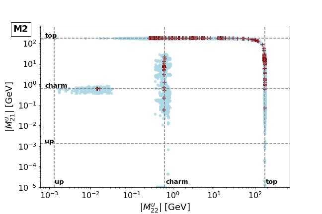
In Fig.Ā 1, we plot the preferred magnitudes for elements (Mu)22subscriptsubscriptš‘€š‘¢22(M_{u})_{22} and (Mu)21subscriptsubscriptš‘€š‘¢21(M_{u})_{21} when fitting MMs. The red parameter points correspond to a region of parameter space with all deviations below 1ā€‹Ļƒ1šœŽ1\sigma, while blue points have a deviation below 3ā€‹Ļƒ3šœŽ3\sigma. In the plot, we see a strong preference toward either (Mu)22subscriptsubscriptš‘€š‘¢22(M_{u})_{22} or (Mu)21subscriptsubscriptš‘€š‘¢21(M_{u})_{21} being of the order of the top mass. Similar features can be found in the down sector when plotting (Md)23subscriptsubscriptš‘€š‘‘23(M_{d})_{23} as a function of (Md)22subscriptsubscriptš‘€š‘‘22(M_{d})_{22}.

Refer to caption
Figure 1: Preferred magnitudes for elements of the up quark mass matrix in the flavor basis for model M2. Red crosses correspond to regions with all deviations below 1ā€‹Ļƒ1šœŽ1\sigma, and blue to deviations below 3ā€‹Ļƒ3šœŽ3\sigma.

III.1.3 Models M3a and M3b

For model M3a, the textures are given by

Ī“1:(ƗƗ0ƗƗ000Ɨ)Ī“2:(000000ƗƗ0)Ī”1:(ƗƗ0ƗƗ000Ɨ)Ī”2:(00Ɨ00Ɨ000).:subscriptĪ“1matrix0000subscriptĪ“2:matrix0000000subscriptĪ”1:matrix0000subscriptĪ”2:matrix0000000\displaystyle\begin{split}\Gamma_{1}&:\begin{pmatrix}\times&\times&\makebox[0.0pt][c]{0}\\ \times&\times&\makebox[0.0pt][c]{0}\\ \makebox[0.0pt][c]{0}&\makebox[0.0pt][c]{0}&\times\end{pmatrix}\hskip 5.69054pt\Gamma_{2}:\begin{pmatrix}\makebox[0.0pt][c]{0}&\makebox[0.0pt][c]{0}&\makebox[0.0pt][c]{0}\\ \makebox[0.0pt][c]{0}&\makebox[0.0pt][c]{0}&\makebox[0.0pt][c]{0}\\ \times&\times&\makebox[0.0pt][c]{0}\end{pmatrix}\hskip 5.69054pt\\ \Delta_{1}&:\begin{pmatrix}\times&\times&\makebox[0.0pt][c]{0}\\ \times&\times&\makebox[0.0pt][c]{0}\\ \makebox[0.0pt][c]{0}&\makebox[0.0pt][c]{0}&\times\end{pmatrix}\hskip 4.2679pt\Delta_{2}:\begin{pmatrix}\makebox[0.0pt][c]{0}&\makebox[0.0pt][c]{0}&\times\\ \makebox[0.0pt][c]{0}&\makebox[0.0pt][c]{0}&\times\\ \makebox[0.0pt][c]{0}&\makebox[0.0pt][c]{0}&\makebox[0.0pt][c]{0}\end{pmatrix}.\end{split}

For this model, there are again FCNCs in all quark sectors, but this time around, there are further restrictions. With the charges of the first two generations being degenerate for all quarks, i.e.Ā q1=q2subscriptš‘ž1subscriptš‘ž2q_{1}=q_{2}, u1=u2subscriptš‘¢1subscriptš‘¢2u_{1}=u_{2} and d1=d2subscriptš‘‘1subscriptš‘‘2d_{1}=d_{2}, we have that

ĪžuL=xā€‹šŸ™+(yāˆ’x)ā€‹P3[uL],ĪždL=xā€‹šŸ™+(yāˆ’x)ā€‹Vā€ ā€‹P3[uL]ā€‹V,ĪžuR=(3ā€‹x+y)ā€‹šŸ™+(yāˆ’x)ā€‹P3[uR],ĪždR=āˆ’(x+y)ā€‹šŸ™+(yāˆ’x)ā€‹P3[dR],formulae-sequencesubscriptĪžsubscriptuLš‘„double-struck-šŸ™š‘¦š‘„superscriptsubscriptš‘ƒ3delimited-[]subscriptuLformulae-sequencesubscriptĪžsubscriptdLš‘„double-struck-šŸ™š‘¦š‘„superscriptš‘‰ā€ superscriptsubscriptš‘ƒ3delimited-[]subscriptuLš‘‰formulae-sequencesubscriptĪžsubscriptuR3š‘„š‘¦double-struck-šŸ™š‘¦š‘„superscriptsubscriptš‘ƒ3delimited-[]subscriptš‘¢RsubscriptĪžsubscriptdRš‘„š‘¦double-struck-šŸ™š‘¦š‘„superscriptsubscriptš‘ƒ3delimited-[]subscriptš‘‘R\displaystyle\begin{split}\Xi_{\mathrm{{u_{L}}}}&=x\hskip 1.42262pt\mathbb{1}+(y-x)\hskip 1.42262ptP_{3}^{[\mathrm{{u_{L}}}]},\\ \Xi_{\mathrm{{d_{L}}}}&=x\hskip 1.42262pt\mathbb{1}+(y-x)\hskip 1.42262ptV^{\dagger}P_{3}^{[\mathrm{{u_{L}}}]}V,\\ \Xi_{\mathrm{u_{R}}}&=(3x+y)\hskip 1.42262pt\mathbb{1}+(y-x)\hskip 1.42262ptP_{3}^{[u_{\mathrm{R}}]},\\ \Xi_{\mathrm{d_{R}}}&=-(x+y)\hskip 1.42262pt\mathbb{1}+(y-x)\hskip 1.42262ptP_{3}^{[d_{\mathrm{R}}]},\end{split} (30)

with xā‰ yš‘„š‘¦x\neq y, while, for the scalar-mediated FCNCs,

š’¦u=2v2ā€‹(šŸ™āˆ’P3[uL])ā€‹Duā€‹P3[uR],š’¦d=2v2ā€‹Vā€ ā€‹P3[uL]ā€‹Vā€‹Ddā€‹(šŸ™āˆ’P3[dR]).formulae-sequencesubscriptš’¦š‘¢2subscriptš‘£2double-struck-šŸ™superscriptsubscriptš‘ƒ3delimited-[]subscriptš‘¢Lsubscriptš·š‘¢superscriptsubscriptš‘ƒ3delimited-[]subscriptš‘¢Rsubscriptš’¦š‘‘2subscriptš‘£2superscriptš‘‰ā€ superscriptsubscriptš‘ƒ3delimited-[]subscriptš‘¢Lš‘‰subscriptš·š‘‘double-struck-šŸ™superscriptsubscriptš‘ƒ3delimited-[]subscriptš‘‘R\displaystyle\begin{split}\mathcal{K}_{u}&=\frac{\sqrt{2}}{v_{2}}\left(\mathbb{1}-P_{3}^{[u_{\mathrm{L}}]}\right)D_{u}P_{3}^{[u_{\mathrm{R}}]},\\ \mathcal{K}_{d}&=\frac{\sqrt{2}}{v_{2}}V^{\dagger}P_{3}^{[u_{\mathrm{L}}]}VD_{d}\left(\mathbb{1}-P_{3}^{[d_{\mathrm{R}}]}\right).\end{split} (31)

Model M3b, on the other hand, has the same expression for ĪžĪž\Xi as model M3a, while the scalar-mediated FCNCs are now given by

v22ā€‹š’¦q=(šŸ™āˆ’P3[qL])ā€‹Dqā€‹(šŸ™āˆ’P3[qR])+P3[qL]ā€‹Dqā€‹P3[qR]subscriptš‘£22subscriptš’¦š‘ždouble-struck-šŸ™superscriptsubscriptš‘ƒ3delimited-[]subscriptš‘žLsubscriptš·š‘ždouble-struck-šŸ™superscriptsubscriptš‘ƒ3delimited-[]subscriptš‘žRsuperscriptsubscriptš‘ƒ3delimited-[]subscriptš‘žLsubscriptš·š‘žsuperscriptsubscriptš‘ƒ3delimited-[]subscriptš‘žR\displaystyle\begin{split}\frac{v_{2}}{\sqrt{2}}\mathcal{K}_{q}=(\mathbb{1}-P_{3}^{[q_{\mathrm{L}}]})D_{q}(\mathbb{1}-P_{3}^{[q_{\mathrm{R}}]})+P_{3}^{[q_{\mathrm{L}}]}D_{q}P_{3}^{[q_{\mathrm{R}}]}\end{split} (32)

with q=u,dš‘žš‘¢š‘‘q=u,d.

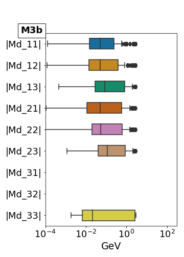
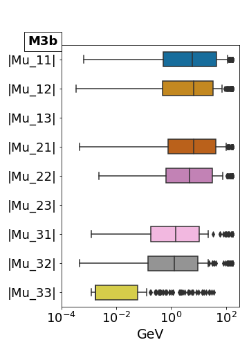
Figure 2 shows the preferred values for elements of the mass matrices. Here we see that, for model M3b, (Mu)33subscriptsubscriptš‘€š‘¢33(M_{u})_{33} prefers having values around the up mass, while the remaining elements have a larger flexibility. The equivalent plot for model M3a shows a strong preference for (Md)33subscriptsubscriptš‘€š‘‘33(M_{d})_{33} to be of the order of the down quark mass.

The figure is a so-called box plot, where the array of data is sorted by magnitude and then split into four equally sized parts, each referred to as a quartile. The black line within the box is the median of the dataset, while the box itself extends from the first to the third quartile. The so-called whiskers span from the smallest to the largest values in the set, out of the points not classified as outliers. An outlier is here defined as any point further away from the first or third quartile than one and a half times the length of the box. For a normal distribution, this would correspond to 0.7% of the data. The outliers are marked as black dots in the figure and, due to the low number of good points in their vicinity, they indicate the fine-tuned regions of the parameter space.
Refer to caption
Refer to caption
Figure 2: Preferred values for the elements of the up quark mass matrix (left) and down quark mass matrix (right) for model M3b. The included parameter points fit the MMs with a deviation below 1ā€‹Ļƒ1šœŽ1\sigma.

For both models M3a and M3b, at most eight out of the 14 Yukawa couplings can be set real from rephasings of the left- and right-handed quarks. There are, hence, 20 parameters in the quark sector, in addition to the three parameters in the lepton sector. One possible choice is for all couplings in Ī“2subscriptĪ“2\Gamma_{2} and Ī”2subscriptĪ”2\Delta_{2} to be real, in addition to the three diagonal couplings in Ī”1subscriptĪ”1\Delta_{1} and (Ī“1)33subscriptsubscriptĪ“133(\Gamma_{1})_{33}.

III.2 Leptons that couple to both Higgs doublets

This section contains all models fulfilling the constraints specified in Sec.Ā II.3, while simultaneously having leptons that couple to both Higgs doublets. Contrary to the models discussed in the previous subsection, the inclusion of charged leptons carrying Uā€‹(1)ā€²š‘ˆsuperscript1ā€²U(1)^{\prime} charge is now crucial for all charge assignments.

III.2.1 Models M4a and M4b

For model M4a, the textures are given by

Ī“1:(000ƗƗ000Ɨ)Ī“2:(ƗƗ000Ɨ000)Ī”1:(00000Ɨ0Ɨ0)Ī”2:(Ɨ0000000Ɨ),:subscriptĪ“1matrix000000subscriptĪ“2:matrix000000subscriptĪ”1:matrix0000000subscriptĪ”2:matrix0000000\displaystyle\begin{split}\Gamma_{1}&:\begin{pmatrix}\makebox[0.0pt][c]{0}&\makebox[0.0pt][c]{0}&\makebox[0.0pt][c]{0}\\ \times&\times&\makebox[0.0pt][c]{0}\\ \makebox[0.0pt][c]{0}&\makebox[0.0pt][c]{0}&\times\end{pmatrix}\hskip 5.69054pt\Gamma_{2}:\begin{pmatrix}\times&\times&\makebox[0.0pt][c]{0}\\ \makebox[0.0pt][c]{0}&\makebox[0.0pt][c]{0}&\times\\ \makebox[0.0pt][c]{0}&\makebox[0.0pt][c]{0}&\makebox[0.0pt][c]{0}\end{pmatrix}\hskip 5.69054pt\\ \Delta_{1}&:\begin{pmatrix}\makebox[0.0pt][c]{0}&\makebox[0.0pt][c]{0}&\makebox[0.0pt][c]{0}\\ \makebox[0.0pt][c]{0}&\makebox[0.0pt][c]{0}&\times\\ \makebox[0.0pt][c]{0}&\times&\makebox[0.0pt][c]{0}\end{pmatrix}\hskip 4.2679pt\Delta_{2}:\begin{pmatrix}\times&\makebox[0.0pt][c]{0}&\makebox[0.0pt][c]{0}\\ \makebox[0.0pt][c]{0}&\makebox[0.0pt][c]{0}&\makebox[0.0pt][c]{0}\\ \makebox[0.0pt][c]{0}&\makebox[0.0pt][c]{0}&\times\end{pmatrix},\end{split}

with the corresponding charges specified in Table 2. Model M4a can have at most eight simultaneously real Yukawa couplings from rephasings of the quark fields. There are, hence, 12 parameters in the quark sector, in addition to the three parameters in the lepton sector. One allowed scenario is for all couplings in Ī“1subscriptĪ“1\Gamma_{1}, Ī”1subscriptĪ”1\Delta_{1} and Ī”2subscriptĪ”2\Delta_{2} to be real, in addition to (Ī“2)11subscriptsubscriptĪ“211(\Gamma_{2})_{11} (similar for M4b).

Since both combinations Muā€‹Muā€ subscriptš‘€š‘¢superscriptsubscriptš‘€š‘¢ā€ M_{u}M_{u}^{\dagger} and Muā€ ā€‹Musuperscriptsubscriptš‘€š‘¢ā€ subscriptš‘€š‘¢M_{u}^{\dagger}M_{u} are real and block diagonal, the diagonalization matrices UuLsubscriptš‘ˆuLU_{\mathrm{uL}} and UuRsubscriptš‘ˆuRU_{\mathrm{uR}} are simply given by a real orthogonal rotation. Using the same notation as in Eq.Ā (12), the rotation angle for UuLsubscriptš‘ˆuLU_{\mathrm{uL}} will be given by

tanā”2ā€‹ĪøuL=2ā€‹(Mu)23ā€‹(Mu)33(Mu)322+(Mu)332āˆ’(Mu)232,2subscriptšœƒuL2subscriptsubscriptš‘€š‘¢23subscriptsubscriptš‘€š‘¢33superscriptsubscriptsubscriptš‘€š‘¢322superscriptsubscriptsubscriptš‘€š‘¢332superscriptsubscriptsubscriptš‘€š‘¢232\displaystyle\begin{split}\tan 2\theta_{\mathrm{uL}}=\frac{2\left(M_{u}\right)_{23}\left(M_{u}\right)_{33}}{\left(M_{u}\right)_{32}^{2}+\left(M_{u}\right)_{33}^{2}-\left(M_{u}\right)_{23}^{2}},\end{split} (33)

and the same for tanā”2ā€‹ĪøuR2subscriptšœƒuR\tan 2\theta_{\mathrm{uR}}, but with (Mu)23subscriptsubscriptš‘€š‘¢23\left(M_{u}\right)_{23} and (Mu)32subscriptsubscriptš‘€š‘¢32\left(M_{u}\right)_{32} exchanged in all places. This can be further simplified by once again using the principal invariants, which has three possible solutions in the up sector, namely

(Mu)11=mc,(Mu)32=muā€‹mt(Mu)23,(Mu)33=((Mu)232āˆ’mu2)ā€‹(mt2āˆ’(Mu)232)(Mu)23,\displaystyle\begin{split}(M_{u})_{11}&=m_{c},\;\;\;\;(M_{u})_{32}=\frac{m_{u}m_{t}}{(M_{u})_{23}},\\ (M_{u})_{33}&=\frac{\sqrt{\Big{(}(M_{u})_{23}^{2}-m_{u}^{2}\Big{)}\Big{(}m_{t}^{2}-(M_{u})_{23}^{2}\Big{)}}}{(M_{u})_{23}},\end{split} (34)

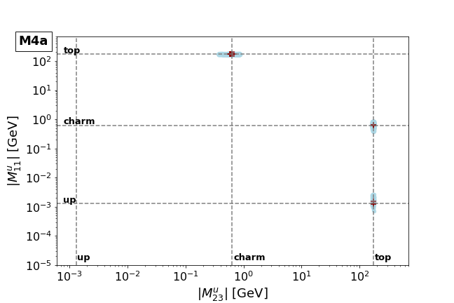
and two equivalent expressions but with the masses exchanged as mcā†”mtā†”subscriptš‘šš‘subscriptš‘šš‘”m_{c}\leftrightarrow m_{t} and mcā†”muā†”subscriptš‘šš‘subscriptš‘šš‘¢m_{c}\leftrightarrow m_{u}. Comparing this with the result of the scan in Fig.Ā 3, we see, as expected, that (Mu)11subscriptsubscriptš‘€š‘¢11(M_{u})_{11} always take on one of the three possible up-type quark masses. The gauge-mediated FCNC couplings are then given by

ĪžuL=xā€‹šŸ™+(yāˆ’x)ā€‹(P2[uL]+2ā€‹P3[uL]),ĪždL=xā€‹šŸ™+(yāˆ’x)ā€‹Vā€ ā€‹(P2[uL]+2ā€‹P3[uL])ā€‹V,ĪžuR=5ā€‹x+7ā€‹y3ā€‹šŸ™+(yāˆ’x)ā€‹(3ā€‹P2[uR]+2ā€‹P3[uR]),ĪždR=xāˆ’7ā€‹y3ā€‹šŸ™+(yāˆ’x)ā€‹P3[dR],formulae-sequencesubscriptĪžuLš‘„double-struck-šŸ™š‘¦š‘„superscriptsubscriptš‘ƒ2delimited-[]subscriptuL2superscriptsubscriptš‘ƒ3delimited-[]subscriptuLformulae-sequencesubscriptĪždLš‘„double-struck-šŸ™š‘¦š‘„superscriptš‘‰ā€ superscriptsubscriptš‘ƒ2delimited-[]subscriptuL2superscriptsubscriptš‘ƒ3delimited-[]subscriptuLš‘‰formulae-sequencesubscriptĪžuR5š‘„7š‘¦3double-struck-šŸ™š‘¦š‘„3superscriptsubscriptš‘ƒ2delimited-[]subscriptuR2superscriptsubscriptš‘ƒ3delimited-[]subscriptuRsubscriptĪždRš‘„7š‘¦3double-struck-šŸ™š‘¦š‘„superscriptsubscriptš‘ƒ3delimited-[]subscriptdR\displaystyle\begin{split}\Xi_{\mathrm{uL}}&=x\hskip 1.42262pt\mathbb{1}+(y-x)\hskip 1.42262pt\big{(}P_{2}^{[\mathrm{u_{L}}]}+2P_{3}^{[\mathrm{u_{L}}]}\big{)},\\ \Xi_{\mathrm{dL}}&=x\hskip 1.42262pt\mathbb{1}+(y-x)\hskip 1.42262ptV^{\dagger}\big{(}P_{2}^{[\mathrm{u_{L}}]}+2P_{3}^{[\mathrm{u_{L}}]}\big{)}V,\\ \Xi_{\mathrm{uR}}&=\frac{5x+7y}{3}\hskip 1.42262pt\mathbb{1}+(y-x)\hskip 1.42262pt\big{(}3P_{2}^{[\mathrm{u_{R}}]}+2P_{3}^{[\mathrm{u_{R}}]}\big{)},\\ \Xi_{\mathrm{dR}}&=\frac{x-7y}{3}\hskip 1.42262pt\mathbb{1}+(y-x)\hskip 1.42262ptP_{3}^{[\mathrm{d_{R}}]},\end{split} (35)

with xā‰ yš‘„š‘¦x\neq y, and the scalar-mediated FCNCs by

š’¦u=2v2ā€‹(P1[uL]ā€‹Duā€‹P1[uR]+P3[uL]ā€‹Duā€‹P3[uR]),š’¦d=2v2ā€‹Vā€ ā€‹(P1[uL]ā€‹Vā€‹Dd+(P2[uL]āˆ’P1[uL])ā€‹Vā€‹Ddā€‹P3[dR]).formulae-sequencesubscriptš’¦š‘¢2subscriptš‘£2superscriptsubscriptš‘ƒ1delimited-[]subscriptš‘¢Lsubscriptš·š‘¢superscriptsubscriptš‘ƒ1delimited-[]subscriptš‘¢Rsuperscriptsubscriptš‘ƒ3delimited-[]subscriptš‘¢Lsubscriptš·š‘¢superscriptsubscriptš‘ƒ3delimited-[]subscriptš‘¢Rsubscriptš’¦š‘‘2subscriptš‘£2superscriptš‘‰ā€ superscriptsubscriptš‘ƒ1delimited-[]subscriptš‘¢Lš‘‰subscriptš·š‘‘superscriptsubscriptš‘ƒ2delimited-[]subscriptš‘¢Lsuperscriptsubscriptš‘ƒ1delimited-[]subscriptš‘¢Lš‘‰subscriptš·š‘‘superscriptsubscriptš‘ƒ3delimited-[]subscriptš‘‘R\displaystyle\begin{split}\mathcal{K}_{u}&=\frac{\sqrt{2}}{v_{2}}\left(P_{1}^{[u_{\mathrm{L}}]}D_{u}P_{1}^{[u_{\mathrm{R}}]}+P_{3}^{[u_{\mathrm{L}}]}D_{u}P_{3}^{[u_{\mathrm{R}}]}\right),\\ \mathcal{K}_{d}&=\frac{\sqrt{2}}{v_{2}}V^{\dagger}\left(P_{1}^{[u_{\mathrm{L}}]}VD_{d}+(P_{2}^{[u_{\mathrm{L}}]}-P_{1}^{[u_{\mathrm{L}}]})VD_{d}P_{3}^{[d_{\mathrm{R}}]}\right).\end{split} (36)

For model M4b, we have a similar scenario but with the roles of the up and down sectors exchanged.
Refer to caption
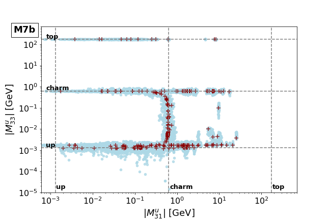
Figure 3: Preferred values for (Mu)23subscriptsubscriptš‘€š‘¢23(M_{u})_{23} and (Mu)11subscriptsubscriptš‘€š‘¢11(M_{u})_{11} for model M4a. Red crosses correspond to regions with all deviations below 1ā€‹Ļƒ1šœŽ1\sigma, and blue ones to deviations below 3ā€‹Ļƒ3šœŽ3\sigma.

III.2.2 Model M5

Next, we have a so-called ā€right model of type Eā€ AlvesĀ etĀ al. (2018), with the textures

Ī“1:(ƗƗ0ƗƗ0ƗƗ0)Ī“2:(00Ɨ00Ɨ00Ɨ)Ī”1:(ƗƗ0ƗƗ0ƗƗ0)Ī”2:(00Ɨ00Ɨ00Ɨ),:subscriptĪ“1matrix000subscriptĪ“2:matrix000000subscriptĪ”1:matrix000subscriptĪ”2:matrix000000\displaystyle\begin{split}\Gamma_{1}&:\begin{pmatrix}\times&\times&\makebox[0.0pt][c]{0}\\ \times&\times&\makebox[0.0pt][c]{0}\\ \times&\times&\makebox[0.0pt][c]{0}\end{pmatrix}\hskip 5.69054pt\Gamma_{2}:\begin{pmatrix}\makebox[0.0pt][c]{0}&\makebox[0.0pt][c]{0}&\times\\ \makebox[0.0pt][c]{0}&\makebox[0.0pt][c]{0}&\times\\ \makebox[0.0pt][c]{0}&\makebox[0.0pt][c]{0}&\times\end{pmatrix}\hskip 5.69054pt\\ \Delta_{1}&:\begin{pmatrix}\times&\times&\makebox[0.0pt][c]{0}\\ \times&\times&\makebox[0.0pt][c]{0}\\ \times&\times&\makebox[0.0pt][c]{0}\end{pmatrix}\hskip 4.2679pt\Delta_{2}:\begin{pmatrix}\makebox[0.0pt][c]{0}&\makebox[0.0pt][c]{0}&\times\\ \makebox[0.0pt][c]{0}&\makebox[0.0pt][c]{0}&\times\\ \makebox[0.0pt][c]{0}&\makebox[0.0pt][c]{0}&\times\end{pmatrix},\end{split}

and with no FCNCs in the left-handed quark sectors, as the charges of all left-handed quarks are degenerate. For the right-handed quarks, on the other hand, there are only two degenerate charges, such that ĪžuRsubscriptĪžuR\Xi_{\mathrm{uR}} and ĪždRsubscriptĪždR\Xi_{\mathrm{dR}} are of the form, respectively,

ĪžuR=yā€‹šŸ™āˆ’3ā€‹(2ā€‹x+y)ā€‹P3[uR],ĪždR=(2ā€‹xāˆ’y)ā€‹šŸ™+3ā€‹(2ā€‹x+y)ā€‹P3[dR].formulae-sequencesubscriptĪžuRš‘¦double-struck-šŸ™32š‘„š‘¦superscriptsubscriptš‘ƒ3delimited-[]uRsubscriptĪždR2š‘„š‘¦double-struck-šŸ™32š‘„š‘¦superscriptsubscriptš‘ƒ3delimited-[]dR\displaystyle\begin{split}\Xi_{\mathrm{uR}}&=y\hskip 1.42262pt\mathbb{1}-3(2x+y)\hskip 1.42262ptP_{3}^{[\mathrm{uR}]},\\ \Xi_{\mathrm{dR}}&=(2x-y)\hskip 1.42262pt\mathbb{1}+3(2x+y)\hskip 1.42262ptP_{3}^{[\mathrm{dR}]}.\end{split} (37)

Similarly, for the scalar sector, we have

š’¦u=2v2ā€‹Duā€‹P3[uR]andš’¦d=2v2ā€‹Ddā€‹P3[dR].formulae-sequencesubscriptš’¦š‘¢2subscriptš‘£2subscriptš·š‘¢superscriptsubscriptš‘ƒ3delimited-[]subscriptš‘¢Randsubscriptš’¦š‘‘2subscriptš‘£2subscriptš·š‘‘superscriptsubscriptš‘ƒ3delimited-[]subscriptš‘‘R\displaystyle\begin{split}\mathcal{K}_{u}=\frac{\sqrt{2}}{v_{2}}D_{u}P_{3}^{[u_{\mathrm{R}}]}\quad\text{and}\quad\mathcal{K}_{d}=\frac{\sqrt{2}}{v_{2}}D_{d}P_{3}^{[d_{\mathrm{R}}]}.\end{split} (38)

As stated at the beginning of this section, for model M5 we use the physical quark masses and mixing matrix as inputs. Since the left-handed quark doublet charges are fully degenerate under Uā€‹(1)ā€²š‘ˆsuperscript1ā€²U(1)^{\prime}, any weak basis transformation (WBT) in this sector will never affect any observable. Therefore, applying the WBT qL0ā†’UuLā€‹qL0ā†’superscriptsubscriptš‘žL0subscriptš‘ˆuLsuperscriptsubscriptš‘žL0q_{\mathrm{L}}^{0}\rightarrow U_{\mathrm{uL}}q_{\mathrm{L}}^{0}, we are instead in the basis

Mu=Duā€‹UuR,Md=Vā€ ā€‹Ddā€‹UdR.formulae-sequencesubscriptš‘€š‘¢subscriptš·š‘¢subscriptš‘ˆuRsubscriptš‘€š‘‘superscriptš‘‰ā€ subscriptš·š‘‘subscriptš‘ˆdR\displaystyle\begin{split}M_{u}=D_{u}U_{\mathrm{uR}},\;\;M_{d}=V^{\dagger}D_{d}U_{\mathrm{dR}}\,.\end{split} (39)

The only free quantities are the right-handed rotation matrices. The Yukawa couplings get, therefore, fully determined by the above mass matrices.

III.2.3 Models M6a and M6b

Model M6a is the familiar BGL model BrancoĀ etĀ al. (1996),

Ī“1:(ƗƗƗƗƗƗ000)Ī“2:(000000ƗƗƗ)Ī”1:(ƗƗ0ƗƗ0000)Ī”2:(00000000Ɨ),:subscriptĪ“1matrix000subscriptĪ“2:matrix000000subscriptĪ”1:matrix00000subscriptĪ”2:matrix00000000\displaystyle\begin{split}\Gamma_{1}&:\begin{pmatrix}\times&\times&\times\\ \times&\times&\times\\ \makebox[0.0pt][c]{0}&\makebox[0.0pt][c]{0}&\makebox[0.0pt][c]{0}\end{pmatrix}\hskip 5.69054pt\Gamma_{2}:\begin{pmatrix}\makebox[0.0pt][c]{0}&\makebox[0.0pt][c]{0}&\makebox[0.0pt][c]{0}\\ \makebox[0.0pt][c]{0}&\makebox[0.0pt][c]{0}&\makebox[0.0pt][c]{0}\\ \times&\times&\times\end{pmatrix}\hskip 5.69054pt\\ \Delta_{1}&:\begin{pmatrix}\times&\times&\makebox[0.0pt][c]{0}\\ \times&\times&\makebox[0.0pt][c]{0}\\ \makebox[0.0pt][c]{0}&\makebox[0.0pt][c]{0}&\makebox[0.0pt][c]{0}\end{pmatrix}\hskip 4.2679pt\Delta_{2}:\begin{pmatrix}\makebox[0.0pt][c]{0}&\makebox[0.0pt][c]{0}&\makebox[0.0pt][c]{0}\\ \makebox[0.0pt][c]{0}&\makebox[0.0pt][c]{0}&\makebox[0.0pt][c]{0}\\ \makebox[0.0pt][c]{0}&\makebox[0.0pt][c]{0}&\times\end{pmatrix},\end{split}

with the corresponding charges specified in Table 2 and with FCNCs only in the left-handed down sector.

As is well known for BGL-type models, UuLsubscriptš‘ˆuLU_{\mathrm{uL}} and UuRsubscriptš‘ˆuRU_{\mathrm{uR}} are block diagonal. In the right-handed down sector, all charges are degenerate, leading to a diagonal ĪždRsubscriptĪždR\Xi_{\mathrm{dR}}. For the other three quark sectors, on the other hand, there are two degenerate charges yielding

ĪžuL=xā€‹šŸ™+(yāˆ’x)ā€‹Pa,ĪždL=xā€‹šŸ™+(yāˆ’x)ā€‹Vā€ ā€‹Paā€‹V,ĪžuR=23ā€‹(5ā€‹x+y)ā€‹šŸ™+2ā€‹(yāˆ’x)ā€‹Pa,formulae-sequencesubscriptĪžuLš‘„double-struck-šŸ™š‘¦š‘„subscriptš‘ƒš‘Žformulae-sequencesubscriptĪždLš‘„double-struck-šŸ™š‘¦š‘„superscriptš‘‰ā€ subscriptš‘ƒš‘Žš‘‰subscriptĪžuR235š‘„š‘¦double-struck-šŸ™2š‘¦š‘„subscriptš‘ƒš‘Ž\displaystyle\begin{split}\Xi_{\mathrm{uL}}&=x\hskip 1.42262pt\mathbb{1}+(y-x)\hskip 1.42262ptP_{a},\\ \Xi_{\mathrm{dL}}&=x\hskip 1.42262pt\mathbb{1}+(y-x)\hskip 1.42262ptV^{\dagger}P_{a}V,\\ \Xi_{\mathrm{uR}}&=\frac{2}{3}(5x+y)\hskip 1.42262pt\mathbb{1}+2(y-x)\hskip 1.42262ptP_{a},\end{split} (40)

with the projector index a=1,2,3š‘Ž123a=1,2,3 for when (Mu)33=mu,mc,mtsubscriptsubscriptš‘€š‘¢33subscriptš‘šš‘¢subscriptš‘šš‘subscriptš‘šš‘”(M_{u})_{33}=m_{u},m_{c},m_{t}, respectively. For the scalar-mediated FCNCs, we have

š’¦u=2v2ā€‹Paā€‹Duandš’¦d=2v2ā€‹Vā€ ā€‹Paā€‹Vā€‹Dd,formulae-sequencesubscriptš’¦š‘¢2subscriptš‘£2subscriptš‘ƒš‘Žsubscriptš·š‘¢andsubscriptš’¦š‘‘2subscriptš‘£2superscriptš‘‰ā€ subscriptš‘ƒš‘Žš‘‰subscriptš·š‘‘\displaystyle\begin{split}\mathcal{K}_{u}=\frac{\sqrt{2}}{v_{2}}P_{a}D_{u}\quad\text{and}\quad\mathcal{K}_{d}=\frac{\sqrt{2}}{v_{2}}V^{\dagger}P_{a}VD_{d}\,,\end{split} (41)

with aš‘Ža defined as before.

Model M6b obeys similar relations, but with the role of the up and down sectors exchanged. Here the FCNCs are instead limited to the left-handed up sector. For models M6a and M6b, there are, hence, no new parameters.

Here, we can again choose a basis in which the expressions for the mass matrices are simplified. Besides the WBT used for model M5, we can now transform also the right-handed quarks such that in the new basis

Mu=Du,Md=Vā€ ā€‹Dd,formulae-sequencesubscriptš‘€š‘¢subscriptš·š‘¢subscriptš‘€š‘‘superscriptš‘‰ā€ subscriptš·š‘‘\displaystyle\begin{split}M_{u}=D_{u},\;\;M_{d}=V^{\dagger}D_{d}\,,\end{split} (42)

without influencing the conserved currents, due to the way the degeneracy of charges coincides with the block diagonality of the right-handed mixing matrices.

III.2.4 Models M7a and M7b

Finally, model M7a has the textures

Ī“1:(Ɨ00Ɨ0000Ɨ)Ī“2:(0Ɨ00Ɨ0Ɨ00)Ī”1:(00Ɨ00ƗƗƗ0)Ī”2:(ƗƗ0ƗƗ0000),:subscriptĪ“1matrix000000subscriptĪ“2:matrix000000subscriptĪ”1:matrix00000subscriptĪ”2:matrix00000\displaystyle\begin{split}\Gamma_{1}&:\begin{pmatrix}\times&\makebox[0.0pt][c]{0}&\makebox[0.0pt][c]{0}\\ \times&\makebox[0.0pt][c]{0}&\makebox[0.0pt][c]{0}\\ \makebox[0.0pt][c]{0}&\makebox[0.0pt][c]{0}&\times\end{pmatrix}\hskip 5.69054pt\Gamma_{2}:\begin{pmatrix}\makebox[0.0pt][c]{0}&\times&\makebox[0.0pt][c]{0}\\ \makebox[0.0pt][c]{0}&\times&\makebox[0.0pt][c]{0}\\ \times&\makebox[0.0pt][c]{0}&\makebox[0.0pt][c]{0}\end{pmatrix}\hskip 5.69054pt\\ \Delta_{1}&:\begin{pmatrix}\makebox[0.0pt][c]{0}&\makebox[0.0pt][c]{0}&\times\\ \makebox[0.0pt][c]{0}&\makebox[0.0pt][c]{0}&\times\\ \times&\times&\makebox[0.0pt][c]{0}\end{pmatrix}\hskip 4.2679pt\Delta_{2}:\begin{pmatrix}\times&\times&\makebox[0.0pt][c]{0}\\ \times&\times&\makebox[0.0pt][c]{0}\\ \makebox[0.0pt][c]{0}&\makebox[0.0pt][c]{0}&\makebox[0.0pt][c]{0}\end{pmatrix},\end{split}

with the corresponding charges specified in Table 2 and with FCNCs in all quark sectors. Here, there are two degenerate charges in all quark sectors except for the right-handed down quarks, such that the FCNC sources in the gauge sector are given by

ĪžuL=xā€‹šŸ™+(yāˆ’x)ā€‹P3[uL],ĪždL=xā€‹šŸ™+(yāˆ’x)ā€‹Vā€ ā€‹P3[uL]ā€‹V,ĪžuR=7ā€‹x+5ā€‹y3ā€‹šŸ™āˆ’(yāˆ’x)ā€‹P3[uR],ĪždR=āˆ’4ā€‹x+2ā€‹y3ā€‹šŸ™+(yāˆ’x)ā€‹(P3[uR]āˆ’P2[uR]),formulae-sequencesubscriptĪžuLš‘„double-struck-šŸ™š‘¦š‘„superscriptsubscriptš‘ƒ3delimited-[]subscriptuLformulae-sequencesubscriptĪždLš‘„double-struck-šŸ™š‘¦š‘„superscriptš‘‰ā€ superscriptsubscriptš‘ƒ3delimited-[]subscriptuLš‘‰formulae-sequencesubscriptĪžuR7š‘„5š‘¦3double-struck-šŸ™š‘¦š‘„superscriptsubscriptš‘ƒ3delimited-[]subscriptuRsubscriptĪždR4š‘„2š‘¦3double-struck-šŸ™š‘¦š‘„superscriptsubscriptš‘ƒ3delimited-[]subscriptuRsuperscriptsubscriptš‘ƒ2delimited-[]subscriptuR\displaystyle\begin{split}\Xi_{\mathrm{uL}}&=x\hskip 1.42262pt\mathbb{1}+(y-x)\hskip 1.42262ptP_{3}^{[\mathrm{u_{L}}]},\\ \Xi_{\mathrm{dL}}&=x\hskip 1.42262pt\mathbb{1}+(y-x)\hskip 1.42262ptV^{\dagger}P_{3}^{[\mathrm{u_{L}}]}V,\\ \Xi_{\mathrm{uR}}&=\frac{7x+5y}{3}\hskip 1.42262pt\mathbb{1}-(y-x)\hskip 1.42262ptP_{3}^{[\mathrm{u_{R}}]},\\ \Xi_{\mathrm{dR}}&=-\frac{4x+2y}{3}\hskip 1.42262pt\mathbb{1}+(y-x)\hskip 1.42262pt(P_{3}^{[\mathrm{u_{R}}]}-P_{2}^{[\mathrm{u_{R}}]}),\end{split} (43)

with xā‰ yš‘„š‘¦x\neq y, while for the scalar-sector we get

v22ā€‹š’¦u=(šŸ™āˆ’P3[uL])ā€‹Duā€‹(šŸ™āˆ’P3[uR]),v22ā€‹š’¦d=Ddā€‹P2[dR]āˆ’Vā€ ā€‹P3[uL]ā€‹Vā€‹Ddā€‹(P1[dR]āˆ’P2[dR]).formulae-sequencesubscriptš‘£22subscriptš’¦š‘¢double-struck-šŸ™superscriptsubscriptš‘ƒ3delimited-[]subscriptš‘¢Lsubscriptš·š‘¢double-struck-šŸ™superscriptsubscriptš‘ƒ3delimited-[]subscriptš‘¢Rsubscriptš‘£22subscriptš’¦š‘‘subscriptš·š‘‘superscriptsubscriptš‘ƒ2delimited-[]subscriptš‘‘Rsuperscriptš‘‰ā€ superscriptsubscriptš‘ƒ3delimited-[]subscriptš‘¢Lš‘‰subscriptš·š‘‘superscriptsubscriptš‘ƒ1delimited-[]subscriptš‘‘Rsuperscriptsubscriptš‘ƒ2delimited-[]subscriptš‘‘R\displaystyle\begin{split}\frac{v_{2}}{\sqrt{2}}\mathcal{K}_{u}&=(\mathbb{1}-P_{3}^{[u_{\mathrm{L}}]})D_{u}(\mathbb{1}-P_{3}^{[u_{\mathrm{R}}]}),\\ \frac{v_{2}}{\sqrt{2}}\mathcal{K}_{d}&=D_{d}P_{2}^{[d_{\mathrm{R}}]}-V^{\dagger}P_{3}^{[u_{\mathrm{L}}]}VD_{d}(P_{1}^{[d_{\mathrm{R}}]}-P_{2}^{[d_{\mathrm{R}}]}).\end{split} (44)

Model M7b obeys similar relations but with the down and up sector exchanged. In Fig.Ā 4, we show the preferred values for entries of the up quark mass matrices, where red crosses correspond to regions with all deviations below 1ā€‹Ļƒ1šœŽ1\sigma, and blue points to a deviation below 3ā€‹Ļƒ3šœŽ3\sigma. Similar features can be found in the down sector of M7a.

For models M7a and M7b, there are, at most, nine out of 14 Yukawa couplings that can be set real from rephasings of the quark fields. As such, there are 19 parameters in the quark sector. One allowed selection of real entries correspond to all couplings in Ī“2subscriptĪ“2\Gamma_{2} and Ī”2subscriptĪ”2\Delta_{2}, in addition to (Ī”1)12subscriptsubscriptĪ”112(\Delta_{1})_{12} and (Ī”1)31subscriptsubscriptĪ”131(\Delta_{1})_{31}.

Refer to caption
Figure 4: Preferred values for (Mu)33subscriptsubscriptš‘€š‘¢33(M_{u})_{33} and (Mu)31subscriptsubscriptš‘€š‘¢31(M_{u})_{31} in model M7b. Here, red crosses correspond to parameter points with all deviations smaller than 1ā€‹Ļƒ1šœŽ1\sigma, and blue ones to all deviations below 3ā€‹Ļƒ3šœŽ3\sigma.

III.3 Model tendencies

The overall tendencies for fitting the quark MMs for the models are gathered in Table 3. Here, the second column displays the sum of all Ļ‡2superscriptšœ’2\chi^{2} for the very best point for each model, where we see that all models contain regions in parameter space with an excellent agreement with the quarks MMs. The third column instead presents the percentage of points with an individual Ļ‡2superscriptšœ’2\chi^{2} below one, from which we can tell that model M3a has the most preferable landscape, while model M4a has the least preferable one. And, finally, the fourth column presents the two most difficult observables to fit. For most models, this is the strange mass. Note that the largest individual deviation is still always below 5ā€‹Ļƒ5šœŽ5\sigma.

Model Ļ‡mā€‹iā€‹n2subscriptsuperscriptšœ’2š‘šš‘–š‘›\chi^{2}_{min} Ļ‡i2<1superscriptsubscriptšœ’š‘–21\chi_{i}^{2}<1 1ā‰¤Ļ‡i2ā‰¤251superscriptsubscriptšœ’š‘–2251\leq\chi_{i}^{2}\leq 25
M2 1.4Ɨ10āˆ’31.4superscript1031.4\times 10^{-3} 77%percent7777\% 78%ā€‹[ms]9%ā€‹[md]percent78delimited-[]subscriptš‘šš‘ percent9delimited-[]subscriptš‘šš‘‘\begin{array}[]{l}78\%\;[m_{s}]\\ 9\%\;\;\;[m_{d}]\end{array}
M3a 1.8Ɨ10āˆ’31.8superscript1031.8\times 10^{-3} 93%percent9393\% 64%ā€‹[mb]23%ā€‹[ms]percent64delimited-[]subscriptš‘šš‘percent23delimited-[]subscriptš‘šš‘ \begin{array}[]{l}64\%\;[m_{b}]\\ 23\%\;[m_{s}]\end{array}
M3b 4.2Ɨ10āˆ’34.2superscript1034.2\times 10^{-3} 88%percent8888\% 33%ā€‹[md]20%ā€‹[ms,b]percent33delimited-[]subscriptš‘šš‘‘percent20delimited-[]subscriptš‘šš‘ š‘\begin{array}[]{l}33\%\;[m_{d}]\\ 20\%\;[m_{s,b}]\end{array}
M4a 3.8Ɨ10āˆ’33.8superscript1033.8\times 10^{-3} 60%percent6060\% 84%ā€‹[ms]11%ā€‹[|Vtā€‹d|]percent84delimited-[]subscriptš‘šš‘ percent11delimited-[]subscriptš‘‰š‘”š‘‘\begin{array}[]{l}84\%\;[m_{s}]\\ 11\%\;[|V_{td}|]\end{array}
M4b 4.5Ɨ10āˆ’34.5superscript1034.5\times 10^{-3} 77%percent7777\% 70%ā€‹[mc]17%ā€‹[mt]percent70delimited-[]subscriptš‘šš‘percent17delimited-[]subscriptš‘šš‘”\begin{array}[]{l}70\%\;[m_{c}]\\ 17\%\;[m_{t}]\end{array}
M7a 2.9Ɨ10āˆ’32.9superscript1032.9\times 10^{-3} 88%percent8888\% 89%ā€‹[ms]11%ā€‹[mc]percent89delimited-[]subscriptš‘šš‘ percent11delimited-[]subscriptš‘šš‘\begin{array}[]{l}89\%\;[m_{s}]\\ 11\%\;[m_{c}]\end{array}
M7b 1.8Ɨ10āˆ’31.8superscript1031.8\times 10^{-3} 81%percent8181\% 67%ā€‹[ms]9%ā€‹[mt,u]percent67delimited-[]subscriptš‘šš‘ percent9delimited-[]subscriptš‘šš‘”š‘¢\begin{array}[]{l}67\%\;[m_{s}]\\ 9\%\;\;\;[m_{t,u}]\end{array}
Table 3: Display of the effort required for fitting MMs for the various models. The second column presents the total Ļ‡2superscriptšœ’2\chi^{2} of the best-fit point, the third column shows the percentage of points with a Ļ‡2superscriptšœ’2\chi^{2} below one, and the fourth column gives the observables with the most significant deviations from the data, for the points with a deviation in the range 1ā€‹Ļƒ1šœŽ1\sigma-5ā€‹Ļƒ5šœŽ5\sigma.

IV Scan and phenomenological tests

In this section, we present the details on the scan performed for each of the models found in Sec.Ā III. For all models except M5 and M6, we have given as input the values of the best-fit points from the masses and mixing scan. We are then left to range over:

  • ā€¢

    neutral Zā€²superscriptš‘ā€²Z^{\prime} gauge coupling gā€²āˆˆ[5Ɨ10āˆ’4,1]superscriptš‘”ā€²5superscript1041g^{\prime}\in[5\times 10^{-4},1];

  • ā€¢

    scalar singlet VEV vSāˆˆ[102,106]subscriptš‘£š‘†superscript102superscript106v_{S}\in[10^{2},10^{6}] GeV;

  • ā€¢

    dimensionless scalar parameters Ī»12,S,Sā€‹iāˆˆ[āˆ’1,1]subscriptšœ†12š‘†š‘†š‘–11\lambda_{12,S,Si}\in[-1,1]; and

  • ā€¢

    dimensionful scalar parameter a1āˆˆ[āˆ’5,5]subscriptš‘Ž155a_{1}\in[-5,5] TeV.

The mass parameters mi2superscriptsubscriptš‘šš‘–2m_{i}^{2} and mS2superscriptsubscriptš‘šš‘†2m_{S}^{2} are fixed by the tadpole conditions, while sĪøsubscriptš‘ šœƒs_{\theta} and fš‘“f are left as free parameters (for more details, see Sec.Ā IV.1). In the scan, we compute the masses for the neutral gauge bosons, neutral and charged scalars and their respective couplings to fermions and bosons. With that information, we then compute their corrections to a set of physical observables detailed below.

For models M5 and M6, the approach is slightly different. As explained in the previous section, there is no need to perform a masses and mixing scan since these parameters can be given as input. In model M6, the Yukawa sector is fully determined by the known quark masses and CKM mixing, such that the only new free parameter is tanā”Ī²š›½\tan\beta, for which we choose Ī²š›½\beta to be in the interval [10āˆ’3,1.56]superscript1031.56[10^{-3},1.56]. In model M5, we can once more set the quarksā€™ masses and mixing to the physical ones, but we are still left with two generic unitary matrices in the up and down right-handed quark sectors. These unitary matrices are parameterized as VR=Kā€‹R12ā€‹R13ā€‹R23subscriptš‘‰š‘…š¾subscriptš‘…12subscriptš‘…13subscriptš‘…23V_{R}=KR_{12}R_{13}R_{23}, with Kš¾K a diagonal matrix with three phases bounded by [10āˆ’1,2Ļ€[[10^{-1},2\pi[ and Riā€‹jsubscriptš‘…š‘–š‘—R_{ij} a complex rotation in the iā€‹jš‘–š‘—ij plane with both the angle and phase constrained to the interval [10āˆ’5,2Ļ€[[10^{-5},2\pi[.

Next, we give a more detailed description of the observables used in the scan.

IV.1 Electroweak and low-energy constraints

As already discussed in Sec.Ā II, the presence of mixing between the ā€would-beā€ SM Z^^š‘\hat{Z} and the new gauge boson Z^ā€²superscript^š‘ā€²\hat{Z}^{\prime} will, in turn, lead to modifications on the currents of the physical Zš‘Z boson. The electroweak sector of the SM has been probed with a very high level of accuracy, such that only a very small mixing is, in general, allowed. In our study of the EW constraints, we look at the Zš‘Z-pole pseudo-observables

Ī“Ztot:Z total decay width,Ļƒhad:e+ā€‹eāˆ’ā€‹cross section to hadrons,Af:parity-violating assym.Ā ā€‹f={b,c,s,l},AfFB:forward-backward assym.Ā ā€‹f={b,c,s,l},Rf:partial width ratiosĀ ā€‹f={b,c,l}.:superscriptsubscriptĪ“š‘totZ total decay widthsubscriptšœŽhad:superscriptš‘’superscriptš‘’cross section to hadronssubscriptš“š‘“:parity-violating assym.Ā š‘“š‘š‘š‘ š‘™superscriptsubscriptš“š‘“FB:forward-backward assym.Ā š‘“š‘š‘š‘ š‘™subscriptš‘…š‘“:partial width ratiosĀ š‘“š‘š‘š‘™\displaystyle\begin{split}\Gamma_{Z}^{\mathrm{tot}}:&\quad\text{Z total decay width}\,,\\ \sigma_{\mathrm{had}}:&\quad e^{+}e^{-}\text{cross section to hadrons}\,,\\ A_{f}:&\quad\text{parity-violating assym. }f=\{b,c,s,l\}\,,\\ A_{f}^{\mathrm{FB}}:&\quad\text{forward-backward assym. }f=\{b,c,s,l\}\,,\\ R_{f}:&\quad\text{partial width ratios }f=\{b,c,l\}\,.\end{split}

To compute these observables, we follow closely the Leptop computer programĀ NovikovĀ etĀ al. (1995a, b) approach, which includes one-loop EW corrections. In this approach Ī±ĀÆĀÆš›¼\bar{\alpha}, mZsubscriptš‘šš‘m_{Z} and GFsubscriptšŗš¹G_{F} are given as inputs, where GFsubscriptšŗš¹G_{F} is the Fermi coupling constant. However, since the presence of the new Zā€²superscriptš‘ā€²Z^{\prime} boson alters the Zš‘Z mass, we include mZsubscriptš‘šš‘m_{Z} and Ī±ĀÆĀÆš›¼\bar{\alpha} in the fit. We then take

sĪø2ā€‹cĪø2=Ļ€ā€‹Ī±ĀÆ2ā€‹GFā€‹mZ2superscriptsubscriptš‘ šœƒ2superscriptsubscriptš‘šœƒ2šœ‹ĀÆš›¼2subscriptšŗš¹superscriptsubscriptš‘šZ2\displaystyle s_{\theta}^{2}c_{\theta}^{2}=\frac{\pi\bar{\alpha}}{\sqrt{2}G_{F}m_{\mathrm{Z}}^{2}} (45)

as the defining relation for sĪøsubscriptš‘ šœƒs_{\theta}, where Ī±ĀÆĀÆš›¼\bar{\alpha} includes the running due to the three lepton and five ā€lightā€ quark loops leading to Ī±ĀÆāˆ’1ā‰”Ī±ā€‹(mZ2)āˆ’1=128.878Ā±0.090superscriptĀÆš›¼1š›¼superscriptsuperscriptsubscriptš‘šš‘21plus-or-minus128.8780.090\bar{\alpha}^{-1}\equiv\alpha(m_{Z}^{2})^{-1}=128.878\pm 0.090Ā NovikovĀ etĀ al. (1995b). The analytical definitions for these pseudo-observables are the standard ones, and their one-loop corrections can be found in Refs.Ā NovikovĀ etĀ al. (1995a, b). The effects of the scalars were taken into account through the computation of the oblique parametersĀ GrimusĀ etĀ al. (2008), along the same lines as BurgessĀ BurgessĀ etĀ al. (1994).

We also compute the off-pole cross sections with both Zš‘Z and Zā€²superscriptš‘ā€²Z^{\prime}, for the final states Ī¼+ā€‹Ī¼āˆ’superscriptšœ‡superscriptšœ‡\mu^{+}\mu^{-}, Ļ„+ā€‹Ļ„āˆ’superscriptšœsuperscriptšœ\tau^{+}\tau^{-} and qā€‹qĀÆš‘žĀÆš‘žq\bar{q}, within the energy range s=[130,207]š‘ 130207\sqrt{s}=[130,207] GeV given by LEP-IIĀ SchaelĀ etĀ al. (2013).

The previous observables do not really constrain the interactions of the Zš‘Z boson with the top quark. We have therefore included also the top width in the fit, in addition to the rare top decays tā†’Zā€‹qā†’š‘”š‘š‘žt\rightarrow Zq and tā†’hā€‹qā†’š‘”ā„Žš‘žt\rightarrow hq.

Low-energy constraints such as atomic parity violation, electric dipole moments (EDMs), and the muon magnetic moment can place significant bounds on the parameter space of our scenarios. Atomic parity violation for Cs55133superscriptsubscriptCs55133{}^{133}_{\hskip 4.26773pt55}\mathrm{Cs} and Tl81205superscriptsubscriptTl81205{}^{205}_{\hskip 4.26773pt81}\mathrm{Tl} have been included in the fitĀ ErlerĀ etĀ al. (2003); GingesĀ andĀ Flambaum (2004). For the neutron EDM, we have considered one-loop corrections from neutral and charged scalarsĀ JungĀ andĀ Pich (2014) and Barr-Zee diagramsĀ BarrĀ andĀ Zee (1990); AbeĀ etĀ al. (2014), while for the muon magnetic moment both the gauge and scalar one-loop contributions are taken into accountĀ JegerlehnerĀ andĀ Nyffeler (2009). The EDM of the electron, on the other hand, is virtually zero since there are no FCNCs in the lepton sector.

IV.2 Meson constraints

A flavor-changing mediator, scalar or vector, is strongly constrained from meson observables. In the fit we have included:

Ī”ā€‹MM0:mass splittingĀ BurasĀ etĀ al. (2013a, b, 2014); GolowichĀ etĀ al. (2007, 2009),ĻµK:Kaon sectorĀ Cā€‹PĀ asymmetryĀ BurasĀ etĀ al. (2013a, b, 2014),SĻˆā€‹Ks,SĻˆā€‹Ļ•:B-sectorĀ Cā€‹P-violating obs.Ā BurasĀ etĀ al. (2013a, b, 2014),Bsā†’Ī¼ā€‹Ī¼:leptonic decayĀ BurasĀ etĀ al. (2012, 2013c); DeĀ BruynĀ etĀ al. (2012); AaijĀ etĀ al. (2017a),Bā†’Xsā€‹Ī³:radiative decayĀ MisiakĀ etĀ al. (2015); BurasĀ etĀ al. (2011).:Ī”subscriptš‘€superscriptš‘€0mass splittingĀ BurasĀ etĀ al. (2013a, b, 2014); GolowichĀ etĀ al. (2007, 2009)subscriptitalic-Ļµš¾:Kaon sectorĀ CPĀ asymmetryĀ BurasĀ etĀ al. (2013a, b, 2014)subscriptš‘†šœ“subscriptš¾š‘ subscriptš‘†šœ“italic-Ļ•:ā†’B-sectorĀ CP-violating obs.Ā BurasĀ etĀ al. (2013a, b, 2014)subscriptšµš‘ šœ‡šœ‡:ā†’leptonic decayĀ BurasĀ etĀ al. (2012, 2013c); DeĀ BruynĀ etĀ al. (2012); AaijĀ etĀ al. (2017a)šµsubscriptš‘‹š‘ š›¾:radiative decayĀ MisiakĀ etĀ al. (2015); BurasĀ etĀ al. (2011)\displaystyle\begin{split}\Delta M_{M^{0}}:&\quad\text{mass splitting\leavevmode\nobreak\ \cite[cite]{\@@bibref{Authors Phrase1YearPhrase2}{Buras:2012jb,Buras:2013rqa,Buras:2014zga,Golowich:2007ka,Golowich:2009ii}{\@@citephrase{(}}{\@@citephrase{)}}}}\,,\\ \epsilon_{K}:&\quad\text{Kaon sector $CP$ asymmetry\leavevmode\nobreak\ \cite[cite]{\@@bibref{Authors Phrase1YearPhrase2}{Buras:2012jb,Buras:2013rqa,Buras:2014zga}{\@@citephrase{(}}{\@@citephrase{)}}}}\,,\\ S_{\psi K_{s}}\,,\,S_{\psi\phi}:&\quad\text{$B$-sector $CP$-violating obs.\leavevmode\nobreak\ \cite[cite]{\@@bibref{Authors Phrase1YearPhrase2}{Buras:2012jb,Buras:2013rqa,Buras:2014zga}{\@@citephrase{(}}{\@@citephrase{)}}}}\,,\\ B_{s}\rightarrow\mu\mu:&\quad\text{leptonic decay\leavevmode\nobreak\ \cite[cite]{\@@bibref{Authors Phrase1YearPhrase2}{Buras:2012ru,Buras:2013uqa,DeBruyn:2012wj,Aaij:2017vad}{\@@citephrase{(}}{\@@citephrase{)}}}}\,,\\ B\rightarrow X_{s}\gamma:&\quad\text{radiative decay\leavevmode\nobreak\ \cite[cite]{\@@bibref{Authors Phrase1YearPhrase2}{Misiak:2015xwa,Buras:2011zb}{\@@citephrase{(}}{\@@citephrase{)}}}}\,.\end{split}

The most dominant bounds usually come from the Ī”ā€‹F=2Ī”š¹2\Delta F=2 transitions observables, Ī”ā€‹MM0Ī”subscriptš‘€superscriptš‘€0\Delta M_{M^{0}} and ĻµKsubscriptitalic-Ļµš¾\epsilon_{K}. The SM contribution for the K0superscriptš¾0K^{0} and Bq0subscriptsuperscriptšµ0š‘žB^{0}_{q} systems is dominated by the top-loop box diagrams, while the SM prediction for the D0superscriptš·0D^{0} system is less trivial. The short-distance effects are virtually zero, but long-distance contributions can be sizable (at the level of the current experimental values). However, long-distance effects are plagued with significant hadronic uncertainties, making it difficult to estimate the SM contribution. For this, we follow the approach of Refs.Ā GolowichĀ etĀ al. (2007, 2009) and attribute the experimental values to short-distance NP. This will serve as an upper bound, such that NP contributions do not greatly exceed the current experimental bound. Box diagrams for the charged Higgs were also included in the numerical scan; seeĀ CrivellinĀ etĀ al. (2013) for the general expressions. The hadronic matrix elements for Ī”ā€‹F=2Ī”š¹2\Delta F=2 processes are very important and were included together with the QCD running of the Wilson coefficients from the NP scale down to the meson scale; this was done in line with Refs.Ā BurasĀ etĀ al. (2013a, b, 2014). We took a conservative approach for the meson oscillation observables and for the Kaon sector, with the error for Ī”ā€‹MKĪ”subscriptš‘€š¾\Delta M_{K} taken as 20%percent2020\% of the central valueĀ TanabashiĀ etĀ al. (2018), while for |ĻµK|subscriptitalic-Ļµš¾|\epsilon_{K}| we take the error to be 10%percent1010\%. We also use a 20%percent2020\% error for the Dš·D-meson sector. For the BšµB-meson sector, since it is less sensitive to long-distance contributions, we took the error for the Ī”ā€‹MBqĪ”subscriptš‘€subscriptšµš‘ž\Delta M_{B_{q}} to be on the 5%percent55\% level.

In the scan, we have also included other meson observables that currently act as upper bounds, such as KLā†’Ī¼+ā€‹Ī¼āˆ’ā†’subscriptš¾šæsuperscriptšœ‡superscriptšœ‡K_{L}\rightarrow\mu^{+}\mu^{-}Ā EckerĀ andĀ Pich (1991); IsidoriĀ andĀ Unterdorfer (2004); Dā€™AmbrosioĀ andĀ Kitahara (2017); AaijĀ etĀ al. (2017b), K+ā†’Ļ€+ā€‹Ī½ā€‹Ī½ĀÆā†’superscriptš¾superscriptšœ‹šœˆĀÆšœˆK^{+}\rightarrow\pi^{+}\nu\bar{\nu} and KLā†’Ļ€0ā€‹Ī½ā€‹Ī½ĀÆā†’subscriptš¾šæsuperscriptšœ‹0šœˆĀÆšœˆK_{L}\rightarrow\pi^{0}\nu\bar{\nu}Ā ArtamonovĀ etĀ al. (2008); BobethĀ etĀ al. (2017); BurasĀ etĀ al. (2015), KLā†’Ļ€0ā€‹e+ā€‹eāˆ’ā†’subscriptš¾šæsuperscriptšœ‹0superscriptš‘’superscriptš‘’K_{L}\rightarrow\pi^{0}e^{+}e^{-} and KLā†’Ļ€0ā€‹Ī¼+ā€‹Ī¼āˆ’ā†’subscriptš¾šæsuperscriptšœ‹0superscriptšœ‡superscriptšœ‡K_{L}\rightarrow\pi^{0}\mu^{+}\mu^{-}Ā MesciaĀ etĀ al. (2006); BlankeĀ etĀ al. (2007); BuchallaĀ etĀ al. (2003); Alavi-HaratiĀ etĀ al. (2004, 2000), and Bdā†’ā„“+ā€‹ā„“āˆ’ā†’subscriptšµš‘‘superscriptā„“superscriptā„“B_{d}\rightarrow\ell^{+}\ell^{-} and Bsā†’e+ā€‹eāˆ’,Ļ„+ā€‹Ļ„āˆ’ā†’subscriptšµš‘ superscriptš‘’superscriptš‘’superscriptšœsuperscriptšœB_{s}\rightarrow e^{+}e^{-},\tau^{+}\tau^{-}Ā CrivellinĀ etĀ al. (2013); TanabashiĀ etĀ al. (2018).

The bā†’sā€‹ā„“ā€‹ā„“ā†’š‘š‘ ā„“ā„“b\rightarrow s\ell\ell transitions are very relevant for these classes of models and have gotten the attention of a large community since the 2014 LHCb resultsĀ AaijĀ etĀ al. (2014) seemed to indicate a breaking of lepton universality. There have been several global fit analysesĀ Descotes-GenonĀ etĀ al. (2013); AltmannshoferĀ andĀ Straub (2013, 2015); AlguerĆ³Ā etĀ al. (2019), pointing the preferred region for some of the four-Fermi effective operators. The experimental status is very likely to change in the next couple of years. Currently LHCb reportsĀ AaijĀ etĀ al. (2019)

Brā€‹(Bsā†’Kā€‹Ī¼+ā€‹Ī¼āˆ’)Brā€‹(Bsā†’Kā€‹e+ā€‹eāˆ’)ā‰”RK[1.1,6]=0.846āˆ’0.054āˆ’0.014+0.060+0.016,Brā†’subscriptšµš‘ š¾superscriptšœ‡superscriptšœ‡Brā†’subscriptšµš‘ š¾superscriptš‘’superscriptš‘’subscriptsuperscriptš‘…1.16š¾subscriptsuperscript0.8460.0600.0160.0540.014\displaystyle\begin{split}\frac{\mathrm{Br}(B_{s}\rightarrow K\mu^{+}\mu^{-})}{\mathrm{Br}(B_{s}\rightarrow Ke^{+}e^{-})}\equiv R^{[1.1,6]}_{K}=0.846^{+0.060+0.016}_{-0.054-0.014}\,,\end{split} (46)

suggesting a 2ā€‹Ļƒ2šœŽ2\sigma-3ā€‹Ļƒ3šœŽ3\sigma deviation from the SM, given RK|SMā‰ƒ1+š’Ŗā€‹(mĪ¼2/mb2)similar-to-or-equalsevaluated-atsubscriptš‘…š¾SM1š’Ŗsuperscriptsubscriptš‘ššœ‡2superscriptsubscriptš‘šš‘2\left.R_{K}\right|_{\mathrm{SM}}\simeq 1+\mathcal{O}(m_{\mu}^{2}/m_{b}^{2})Ā HillerĀ andĀ Kruger (2004). The Belle Collaboration also measured this observable and gives values more compatible with the SMĀ AbdesselamĀ etĀ al. (2019a), i.e.

RK[1,6]=0.98āˆ’0.23+0.27Ā±0.06,RK[q2>14.18]=1.11āˆ’0.26+0.29Ā±0.07.formulae-sequencesuperscriptsubscriptš‘…š¾16plus-or-minussubscriptsuperscript0.980.270.230.06superscriptsubscriptš‘…š¾delimited-[]superscriptš‘ž214.18plus-or-minussubscriptsuperscript1.110.290.260.07\displaystyle\begin{split}R_{K}^{[1,6]}&=0.98^{+0.27}_{-0.23}\pm 0.06\,,\\ R_{K}^{[q^{2}>14.18]}&=1.11^{+0.29}_{-0.26}\pm 0.07\,.\end{split} (47)

In addition to these results, the Belle Collaboration has also reported the ratio for the Bsā†’Kāˆ—ā€‹ā„“ā€‹ā„“ā†’subscriptšµš‘ superscriptš¾āˆ—ā„“ā„“B_{s}\rightarrow K^{\ast}\ell\ell decaysĀ AbdesselamĀ etĀ al. (2019b):

RKāˆ—[0.045,1.1]=0.52āˆ’0.26+0.36Ā±0.05,RKāˆ—[1.1,6]=0.96āˆ’0.29+0.45Ā±0.11,RKāˆ—[15,19]=1.18āˆ’0.32+0.52Ā±0.10.formulae-sequencesuperscriptsubscriptš‘…superscriptš¾āˆ—0.0451.1plus-or-minussubscriptsuperscript0.520.360.260.05formulae-sequencesuperscriptsubscriptš‘…superscriptš¾āˆ—1.16plus-or-minussubscriptsuperscript0.960.450.290.11superscriptsubscriptš‘…superscriptš¾āˆ—1519plus-or-minussubscriptsuperscript1.180.520.320.10\displaystyle\begin{split}R_{K^{\ast}}^{[0.045,1.1]}&=0.52^{+0.36}_{-0.26}\pm 0.05\,,\\ R_{K^{\ast}}^{[1.1,6]}&=0.96^{+0.45}_{-0.29}\pm 0.11\,,\\ R_{K^{\ast}}^{[15,19]}&=1.18^{+0.52}_{-0.32}\pm 0.10\,.\end{split} (48)

To compute the contributions of NP to these observables, we start by defining the effective Hamiltonian

ā„‹effbā†’sā€‹ā„“ā€‹ā„“=āˆ’GF2ā€‹Ī±Ļ€ā€‹Vtā€‹bā€‹Vtā€‹sāˆ—ā€‹āˆ‘i(Ciā€‹š’¬i+Ciā€²ā€‹š’¬iā€²),superscriptsubscriptā„‹effā†’š‘š‘ ā„“ā„“subscriptšŗš¹2š›¼šœ‹subscriptš‘‰š‘”š‘superscriptsubscriptš‘‰š‘”š‘ āˆ—subscriptš‘–subscriptš¶š‘–subscriptš’¬š‘–superscriptsubscriptš¶š‘–ā€²superscriptsubscriptš’¬š‘–ā€²\displaystyle\mathcal{H}_{\mathrm{eff}}^{b\rightarrow s\ell\ell}=-\frac{G_{F}}{\sqrt{2}}\frac{\alpha}{\pi}V_{tb}V_{ts}^{\ast}\sum_{i}\left(C_{i}\mathcal{Q}_{i}+C_{i}^{\prime}\mathcal{Q}_{i}^{\prime}\right)\,, (49)

with

š’¬9(ā€²)=(sĀÆā€‹Ī³Ī¼ā€‹PLā€‹(R)ā€‹b)ā€‹(ā„“ĀÆā€‹Ī³Ī¼ā€‹ā„“),š’¬10(ā€²)=(sĀÆā€‹Ī³Ī¼ā€‹PLā€‹(R)ā€‹b)ā€‹(ā„“ĀÆā€‹Ī³Ī¼ā€‹Ī³5ā€‹ā„“).formulae-sequencesuperscriptsubscriptš’¬9ā€²ĀÆš‘ subscriptš›¾šœ‡subscriptš‘ƒšæš‘…š‘ĀÆā„“superscriptš›¾šœ‡ā„“superscriptsubscriptš’¬10ā€²ĀÆš‘ subscriptš›¾šœ‡subscriptš‘ƒšæš‘…š‘ĀÆā„“superscriptš›¾šœ‡subscriptš›¾5ā„“\displaystyle\begin{split}\mathcal{Q}_{9}^{(\prime)}&=(\bar{s}\gamma_{\mu}P_{L(R)}b)(\bar{\ell}\gamma^{\mu}\ell)\,,\\ \mathcal{Q}_{10}^{(\prime)}&=(\bar{s}\gamma_{\mu}P_{L(R)}b)(\bar{\ell}\gamma^{\mu}\gamma_{5}\ell)\,.\end{split} (50)

For the SM Wilson coefficients, we have C9SMā‰ƒāˆ’C10SMā‰ƒ4.2similar-to-or-equalssuperscriptsubscriptš¶9SMsuperscriptsubscriptš¶10SMsimilar-to-or-equals4.2C_{9}^{\mathrm{SM}}\simeq-C_{10}^{\mathrm{SM}}\simeq 4.2 and zero for their primed counterparts. The RKsubscriptš‘…š¾R_{K} and RKāˆ—subscriptš‘…superscriptš¾āˆ—R_{K^{\ast}} ratios are then given byĀ HillerĀ andĀ Schmaltz (2015)

RK/Kāˆ—ā‰ƒ1+Ī”Ā±+Ī£Ā±,similar-to-or-equalssubscriptš‘…š¾superscriptš¾āˆ—1subscriptĪ”plus-or-minussubscriptĪ£plus-or-minus\displaystyle\begin{split}R_{K/K^{\ast}}&\simeq 1+\Delta_{\pm}+\Sigma_{\pm}\,,\end{split} (51)

with Ī”Ā±subscriptĪ”plus-or-minus\Delta_{\pm} the SM-NP interference term and Ī£Ā±subscriptĪ£plus-or-minus\Sigma_{\pm} the pure NP contribution. Their explicit form is given by

Ī”Ā±ā‰ƒ0.24ā€‹Reā€‹{C9āˆ’10Ī¼ā€‹Ī¼,NPĀ±C9āˆ’10ā€²ā£Ī¼ā€‹Ī¼,NP}āˆ’(Ī¼ā†’e)similar-to-or-equalssubscriptĪ”plus-or-minus0.24Replus-or-minussuperscriptsubscriptš¶910šœ‡šœ‡NPsuperscriptsubscriptš¶910ā€²šœ‡šœ‡NPā†’šœ‡š‘’\displaystyle\begin{split}\Delta_{\pm}&\simeq 0.24\,\mathrm{Re}\left\{C_{9-10}^{\mathrm{\mu\mu,NP}}\pm C_{9-10}^{\mathrm{\prime\mu\mu,NP}}\right\}-(\mu\rightarrow e)\end{split} (52)

and

Ī£Ā±ā‰ƒ0.028ā€‹āˆ‘i=9,10|CiĪ¼ā€‹Ī¼,NPĀ±Ciā€²ā£Ī¼ā€‹Ī¼,NP|2āˆ’(Ī¼ā†’e),similar-to-or-equalssubscriptĪ£plus-or-minus0.028subscriptš‘–910superscriptplus-or-minussuperscriptsubscriptš¶š‘–šœ‡šœ‡NPsuperscriptsubscriptš¶š‘–ā€²šœ‡šœ‡NP2ā†’šœ‡š‘’\displaystyle\begin{split}\Sigma_{\pm}&\simeq 0.028\,\sum_{i=9,10}\left|C_{i}^{\mathrm{\mu\mu,NP}}\pm C_{i}^{\mathrm{\prime\mu\mu,NP}}\right|^{2}-(\mu\rightarrow e)\,,\end{split} (53)

where we defined C9āˆ’10(ā€²)ā‰”C9(ā€²)āˆ’C10(ā€²)subscriptsuperscriptš¶ā€²910subscriptsuperscriptš¶ā€²9subscriptsuperscriptš¶ā€²10C^{(\prime)}_{9-10}\equiv C^{(\prime)}_{9}-C^{(\prime)}_{10}. These Wilson coefficients, in our framework, take the form

C9(ā€²)ā£iā€‹j,Nā€‹P=āˆ’v2ā€‹Ļ€Ī±ā€‹Ī»tBsā€‹[(QZ0dLā€‹(R))sā€‹bā€‹(QZ0eR+QZ0eL)iā€‹jmZ02],subscriptsuperscriptš¶ā€²š‘–š‘—š‘š‘ƒ9superscriptš‘£2šœ‹š›¼superscriptsubscriptšœ†š‘”subscriptšµš‘ delimited-[]subscriptsubscriptsuperscriptš‘„subscriptš‘‘šæš‘…superscriptš‘0š‘ š‘subscriptsubscriptsuperscriptš‘„subscriptš‘’š‘…superscriptš‘0subscriptsuperscriptš‘„subscriptš‘’šæsuperscriptš‘0š‘–š‘—superscriptsubscriptš‘šsuperscriptš‘02\displaystyle\begin{split}C^{(\prime)ij,NP}_{9}=-\frac{v^{2}\pi}{\alpha\lambda_{t}^{B_{s}}}\left[\frac{(Q^{d_{L(R)}}_{Z^{0}})_{sb}(Q^{e_{R}}_{Z^{0}}+Q^{e_{L}}_{Z^{0}})_{ij}}{m_{Z^{0}}^{2}}\right]\,,\end{split} (54)

with Ī»tBsā‰”Vtā€‹bā€‹Vtā€‹sāˆ—superscriptsubscriptšœ†š‘”subscriptšµš‘ subscriptš‘‰š‘”š‘superscriptsubscriptš‘‰š‘”š‘ āˆ—\lambda_{t}^{B_{s}}\equiv V_{tb}V_{ts}^{\ast} and Z0={Z,Zā€²}superscriptš‘0š‘superscriptš‘ā€²Z^{0}=\{Z,Z^{\prime}\}, and equivalent for C10subscriptš¶10C_{10}, but with the sign in front QZ0eLsubscriptsuperscriptš‘„subscriptš‘’šæsuperscriptš‘0Q^{e_{L}}_{Z^{0}} flipped. The corresponding results are discussed in Sec.Ā V.3.

The rare decay modes Bā†’{K,Kāˆ—,Xs}ā€‹Ī½ā€‹Ī½ĀÆā†’šµš¾superscriptš¾subscriptš‘‹š‘ šœˆĀÆšœˆB\rightarrow\{K,K^{*},X_{s}\}\nu\bar{\nu} can be important tests for NP. The SM short-distance predictions were computed in Ref.Ā AltmannshoferĀ etĀ al. (2009) and are still an order of magnitude below the experimental boundsĀ BarateĀ etĀ al. (2001); ChenĀ etĀ al. (2007); AubertĀ etĀ al. (2008), leaving plenty of room for NP. We can parameterize the NP effects through the ratios with the SM predictions; see Ref.Ā AltmannshoferĀ etĀ al. (2009).

IV.3 Collider constraints

At the LHC, several direct searches for new neutral gauge and scalar bosons have been performed. As we shall see in the next section, due to the necessity of a large VEV for the scalar singlet Sš‘†S, the new scalar fields tend to be heavier than the Zā€²superscriptš‘ā€²Z^{\prime} and, in most of the models, out of reach for the current colliders. We have therefore looked at only the collider constraints coming from direct searches of the Zā€²superscriptš‘ā€²Z^{\prime} gauge boson.

We follow a simplified approach by working in the narrow width approximation (NWA). For all models, this turns out to be a good approximation in the low mZā€²subscriptš‘šsuperscriptš‘ā€²m_{Z^{\prime}} range, i.e.Ā below a few tens of TeV. Under the NWA we split the cross section under production and decay, i.e.

Ļƒā€‹(pā€‹pā†’Zā€²ā†’X)|NWA=Ļƒā€‹(pā€‹pā†’Zā€²)ā€‹Brā€‹(Zā€²ā†’X),evaluated-atšœŽā†’š‘š‘superscriptš‘ā€²ā†’XNWAšœŽā†’š‘š‘superscriptš‘ā€²Brā†’superscriptš‘ā€²X\displaystyle\begin{split}\left.\sigma(pp\rightarrow Z^{\prime}\rightarrow\mathrm{X})\right|_{\mathrm{NWA}}=\sigma(pp\rightarrow Z^{\prime})\mathrm{Br}(Z^{\prime}\rightarrow\mathrm{X})\,,\end{split} (55)

where the production cross section is given byĀ CarenaĀ etĀ al. (2004); AccomandoĀ etĀ al. (2011)

Ļƒā€‹(pā€‹pā†’Zā€²)=43ā€‹Ļ€2sā€‹āˆ‘qĪ“ā€‹(Zā€²ā†’qā€‹qĀÆ)mZā€²ā€‹Ļ‰qā€‹(s,mZā€²2),šœŽā†’š‘š‘superscriptš‘ā€²43superscriptšœ‹2š‘ subscriptš‘žĪ“ā†’superscriptš‘ā€²š‘žĀÆš‘žsubscriptš‘šsuperscriptš‘ā€²subscriptšœ”š‘žš‘ subscriptsuperscriptš‘š2superscriptš‘ā€²\displaystyle\sigma(pp\rightarrow Z^{\prime})=\frac{4}{3}\frac{\pi^{2}}{s}\sum_{q}\frac{\Gamma(Z^{\prime}\rightarrow q\bar{q})}{m_{Z^{\prime}}}\,\omega_{q}(s,m^{2}_{Z^{\prime}})\,, (56)

with q=u,c,d,s,bš‘žš‘¢š‘š‘‘š‘ š‘q=u,c,d,s,b. The integration over the parton distribution functions is included in the definition of Ļ‰qā€‹(s,mZā€²2)subscriptšœ”š‘žš‘ subscriptsuperscriptš‘š2superscriptš‘ā€²\omega_{q}(s,m^{2}_{Z^{\prime}}) given in Ref.Ā PazĀ andĀ Roy (2018); these were computed using the parton distribution function set NNPDF23_nnlo_as_0119_qedĀ BallĀ etĀ al. (2013).

The experimental studies used in this analysis are presented in Tab.Ā 4.

ā€„ā€„ā€„ā€„ā€„ā€„ā€„Channel mZā€²subscriptš‘šsuperscriptš‘ā€²m_{Z^{\prime}} [GeV] Ā Ā ā€„ā€„ā€„ā€„Collaboration
e+ā€‹eāˆ’,Ī¼+ā€‹Ī¼āˆ’superscriptš‘’superscriptš‘’superscriptšœ‡superscriptšœ‡e^{+}e^{-},\,\mu^{+}\mu^{-} [250,6000] Ā Ā ā€„ā€„ā€„ā€„ ATLAS@13TeVĀ AadĀ etĀ al. (2019)
[150,3500] Ā Ā ā€„ā€„ā€„ā€„ ATLAS@8TeVĀ AadĀ etĀ al. (2014)
[190,3000] Ā Ā ā€„ā€„ā€„ā€„ ATLAS@7TeVĀ AadĀ etĀ al. (2012b)
Ļ„+ā€‹Ļ„āˆ’superscriptšœsuperscriptšœ\tau^{+}\tau^{-} [200,4000] Ā Ā ā€„ā€„ā€„ā€„ ATLAS@13TeVĀ AaboudĀ etĀ al. (2018a)
[500,2500] Ā Ā ā€„ā€„ā€„ā€„ ATLAS@8TeVĀ AadĀ etĀ al. (2015)
tā€‹tĀÆš‘”ĀÆš‘”t\bar{t} [500,5000] Ā Ā ā€„ā€„ā€„ā€„ ATLAS@13TeVĀ AaboudĀ etĀ al. (2019)
[390,5000] Ā Ā ā€„ā€„ā€„ā€„ ATLAS@13TeVĀ AaboudĀ etĀ al. (2018b)
jā€‹jš‘—š‘—jj [570,8100] Ā Ā ā€„ā€„ā€„ā€„ CMS@13TeVĀ Collaboration (2017)
W+ā€‹Wāˆ’superscriptš‘Šsuperscriptš‘ŠW^{+}W^{-} [1190,4100] Ā Ā ā€„ā€„ā€„ā€„ CMS@13TeVĀ SirunyanĀ etĀ al. (2018a)
[550,4000] Ā Ā ā€„ā€„ā€„ā€„ CMS@13TeVĀ SirunyanĀ etĀ al. (2017)
[300,5000] Ā Ā ā€„ā€„ā€„ā€„ ATLAS@13TeVĀ AaboudĀ etĀ al. (2018c)
Zā€‹hā†’Zā€‹bā€‹bĀÆā€‹(cā€‹cĀÆ)ā†’š‘ā„Žš‘š‘ĀÆš‘š‘ĀÆš‘Zh\rightarrow Zb\bar{b}\,(c\bar{c}) [500,5000] Ā Ā ā€„ā€„ā€„ā€„ ATLAS@13TeVĀ collaboration (2017)
Zā€‹Ī³ā†’eā€‹eā€‹(Ī¼ā€‹Ī¼)ā€‹Ī³ā†’š‘š›¾š‘’š‘’šœ‡šœ‡š›¾Z\gamma\rightarrow ee(\mu\mu)\gamma [350,4000] Ā Ā ā€„ā€„ā€„ā€„ CMS@13TeVĀ SirunyanĀ etĀ al. (2018b)
Table 4: LHC direct Zā€²superscriptš‘ā€²Z^{\prime} searches used for the collider constraints in our scans. The first column shows the final state. The second and third columns give the covered Zā€²superscriptš‘ā€²Z^{\prime} mass range and reference, respectively.

V Model constraints and predictions

In this section, we study all models except for M1, as it has no FCNCs and has already been extensively studied elsewhere. For the numerical scans, we needed to fix the free charges of Table 2. The choice made was based on two simple requirements:

  • (a)

    No Zā€²superscriptš‘ā€²Z^{\prime} coupling to electrons, for both left- and right-handed chiralities. This choice helps to avoid the bounds coming from LEP.

  • (b)

    The largest charge in modulus is 1.

Under (a) and (b), we got the following assignments

(x,y,z)M2=13ā€‹(1,0,3),(x,y)M5=112ā€‹(1,1),(x,y)M4a=139ā€‹(10,1),(x,y)M4b=133ā€‹(āˆ’8,1),(x,y)M6a=130ā€‹(āˆ’2,7),(x,y)M6b=124ā€‹(āˆ’4,5),(x,y)M7a=115ā€‹(2,āˆ’7),(x,y)M7b=121ā€‹(4,āˆ’5),(x,y,z)M3ab=13ā€‹(1,āˆ’2,3),formulae-sequencesubscriptš‘„š‘¦š‘§M213103formulae-sequencesubscriptš‘„š‘¦M511211formulae-sequencesubscriptš‘„š‘¦M4a139101formulae-sequencesubscriptš‘„š‘¦M4b13381formulae-sequencesubscriptš‘„š‘¦M6a13027formulae-sequencesubscriptš‘„š‘¦M6b12445formulae-sequencesubscriptš‘„š‘¦M7a11527formulae-sequencesubscriptš‘„š‘¦M7b12145subscriptš‘„š‘¦š‘§M3ab13123\displaystyle\begin{split}&\big{(}x,y,z\big{)}_{\mathrm{M2}}=\frac{1}{3}\big{(}1,0,3\big{)},\hskip 5.69054pt\big{(}x,y\big{)}_{\mathrm{M5}}=\frac{1}{12}\big{(}1,1\big{)},\\[4.2679pt] &\big{(}x,y\big{)}_{\mathrm{M4a}}=\frac{1}{39}\big{(}10,1\big{)},\hskip 5.69054pt\big{(}x,y\big{)}_{\mathrm{M4b}}=\frac{1}{33}\big{(}-8,1\big{)},\\[4.2679pt] &\big{(}x,y\big{)}_{\mathrm{M6a}}=\frac{1}{30}\big{(}-2,7\big{)},\hskip 5.69054pt\big{(}x,y\big{)}_{\mathrm{M6b}}=\frac{1}{24}\big{(}-4,5\big{)},\\[4.2679pt] &\big{(}x,y\big{)}_{\mathrm{M7a}}=\frac{1}{15}\big{(}2,-7\big{)},\hskip 5.69054pt\big{(}x,y\big{)}_{\mathrm{M7b}}=\frac{1}{21}\big{(}4,-5\big{)},\\[4.2679pt] &\big{(}x,y,z\big{)}_{\mathrm{M3ab}}=\frac{1}{3}\big{(}1,-2,3\big{)},\end{split} (57)

with the corresponding charges given in Table 2.

Some general results for these charges are gathered in Fig.Ā 5, Table 5, and Table 6. Figure 5 shows the ability of the various models to fit all observables. Here we see that, for the explored regions of parameter space, models M2, M3a, M3b, M4a, M5, M7a and M7b can all reach low deviations with data. In particular, models M2, M4a and M7b do so without the corresponding parameter points being outliers of the distributions. Surprisingly enough, the BGL model lacks parameter points below āˆ¼3.9ā€‹Ļƒsimilar-toabsent3.9šœŽ\sim 3.9\sigma. This could be understood from the fact that, while the FCNCs are naturally suppressed in the BGL model, they are also fixed, which reduces the flexibility when fitting parameters.
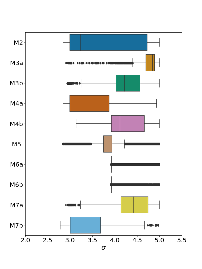
Refer to caption
Figure 5: Figure displaying the ease for the various models in fitting all observational constraints, with the deviation in units of sigma on the xš‘„x axis.

Table 5 displays again the effort required for fitting the various models. Here, we show points with an individual deviation below 5ā€‹Ļƒ5šœŽ5\sigma and mZā€²<30subscriptš‘šsuperscriptš‘ā€²30m_{Z^{\prime}}<30 TeV. The second column contains the number of parameter points, out of the initial 300, that survived this requirement when fitting the MMs. The MM points were then used as input to the minimization of the remaining physical observables, with the number of surviving parameter points shown in the third column. Many of these points share the same MM input but differ in values for the remaining free parameters of the model. Next, the fourth column displays the most constraining collider channels, out of the ones in Table 4. The corresponding channel is displayed only whenever it actually excludes any of the parameter points from the scan, for that corresponding model. Overall, collider constraints are dominated by the Ī¼+ā€‹Ī¼āˆ’superscriptšœ‡superscriptšœ‡\mu^{+}\mu^{-} channel. We recall that for all model implementations chosen, the electron carries no charge under Uā€‹(1)ā€²š‘ˆsuperscript1ā€²U(1)^{\prime}. Finally, the fifth column identifies the observables with the largest individual Ļ‡2superscriptšœ’2\chi^{2}, with the percentages reflecting their relative dominance. For example, for model M4b, 78%percent7878\% of the FIT points had their largest deviation coming from the meson observable Ī”ā€‹MKĪ”subscriptš‘€š¾\Delta M_{K}.

While a more complete scanning of the parameters space would be desirable, the results in Table 5 already show some of the model tendencies. For almost all models, Ī”ā€‹MKĪ”subscriptš‘€š¾\Delta M_{K} is the observable with the highest deviation. However, since the meson sector is plagued with uncertainties on hadronic matrix elements and long-distance contributions, models with deviations around 4ā€‹Ļƒ4šœŽ4\sigma should not be completely discarded. Such sizable deviations in the EW sector are more difficult to accommodate making, for example, model M4a less appealing.

MM FIT Collider
Model points points channel max(Ļ‡i2subscriptsuperscriptšœ’2š‘–\chi^{2}_{i})
M2 264 1.2Ɨ103absentsuperscript103\times 10^{3} ā€“ 64%[Ī”ā€‹MK]27%[Ļƒhad]7%[ĻµK]percent64delimited-[]Ī”subscriptš‘€š¾percent27delimited-[]subscriptšœŽhadpercent7delimited-[]subscriptitalic-Ļµš¾\begin{array}[]{ll}64\%&[\Delta M_{K}]\\ 27\%&[\sigma_{\mathrm{had}}]\\ 7\%&[\epsilon_{K}]\end{array}
M3a 291 8.1Ɨ103absentsuperscript103\times 10^{3} Ī¼+ā€‹Ī¼āˆ’superscriptšœ‡superscriptšœ‡\mu^{+}\mu^{-} 98%[Ī”ā€‹MK]1%[Ī”ā€‹MD]percent98delimited-[]Ī”subscriptš‘€š¾percent1delimited-[]Ī”subscriptš‘€š·\begin{array}[]{ll}98\%&[\Delta M_{K}]\\ 1\%&[\Delta M_{D}]\end{array}
M3b 237 4.7Ɨ103absentsuperscript103\times 10^{3} Ī¼+ā€‹Ī¼āˆ’Ļ„+ā€‹Ļ„āˆ’superscriptšœ‡superscriptšœ‡superscriptšœsuperscriptšœ\begin{array}[]{l}\mu^{+}\mu^{-}\\ \tau^{+}\tau^{-}\end{array} 91%[Ī”ā€‹MK]4%[ĻµK]4%[Ļƒhad]percent91delimited-[]Ī”subscriptš‘€š¾percent4delimited-[]subscriptitalic-Ļµš¾percent4delimited-[]subscriptšœŽhad\begin{array}[]{ll}91\%&[\Delta M_{K}]\\ 4\%&[\epsilon_{K}]\\ 4\%&[\sigma_{\mathrm{had}}]\end{array}
M4a 231 1.4Ɨ103absentsuperscript103\times 10^{3} Ī¼+ā€‹Ī¼āˆ’Ļ„+ā€‹Ļ„āˆ’superscriptšœ‡superscriptšœ‡superscriptšœsuperscriptšœ\begin{array}[]{l}\mu^{+}\mu^{-}\\ \tau^{+}\tau^{-}\end{array} 60%[Ļƒhad]30%[ms]5%[ĻµK]percent60delimited-[]subscriptšœŽhadpercent30delimited-[]subscriptš‘šš‘ percent5delimited-[]subscriptitalic-Ļµš¾\begin{array}[]{ll}60\%&[\sigma_{\mathrm{had}}]\\ 30\%&[m_{s}]\\ 5\%&[\epsilon_{K}]\end{array}
M4b 215 1.8Ɨ103absentsuperscript103\times 10^{3} Ī¼+ā€‹Ī¼āˆ’superscriptšœ‡superscriptšœ‡\mu^{+}\mu^{-} 78%[Ī”ā€‹MK]13%[mc]3%[Ī”ā€‹MD]percent78delimited-[]Ī”subscriptš‘€š¾percent13delimited-[]subscriptš‘šš‘percent3delimited-[]Ī”subscriptš‘€š·\begin{array}[]{ll}78\%&[\Delta M_{K}]\\ 13\%&[m_{c}]\\ 3\%&[\Delta M_{D}]\end{array}
M5 ā€“ 9.6Ɨ103absentsuperscript103\times 10^{3} Ī¼+ā€‹Ī¼āˆ’Ļ„+ā€‹Ļ„āˆ’superscriptšœ‡superscriptšœ‡superscriptšœsuperscriptšœ\begin{array}[]{l}\mu^{+}\mu^{-}\\ \tau^{+}\tau^{-}\end{array} 56%[Ī”ā€‹MK]15%[mZ]7%[Ļƒhad]percent56delimited-[]Ī”subscriptš‘€š¾percent15delimited-[]subscriptš‘šš‘percent7delimited-[]subscriptšœŽhad\begin{array}[]{ll}56\%&[\Delta M_{K}]\\ 15\%&[m_{Z}]\\ 7\%&[\sigma_{\mathrm{had}}]\end{array}
M6a ā€“ 63Ɨ103absentsuperscript103\times 10^{3} Ī¼+ā€‹Ī¼āˆ’Ļ„+ā€‹Ļ„āˆ’Zā€‹hsuperscriptšœ‡superscriptšœ‡superscriptšœsuperscriptšœš‘ā„Ž\begin{array}[]{l}\mu^{+}\mu^{-}\\ \tau^{+}\tau^{-}\\ Zh\end{array} 82%[Ī”ā€‹MK]12%[mZ]3%[Ī“Z]percent82delimited-[]Ī”subscriptš‘€š¾percent12delimited-[]subscriptš‘šš‘percent3delimited-[]subscriptĪ“š‘\begin{array}[]{ll}82\%&[\Delta M_{K}]\\ 12\%&[m_{Z}]\\ 3\%&[\Gamma_{Z}]\end{array}
M6b ā€“ 16Ɨ103absentsuperscript103\times 10^{3} Ī¼+ā€‹Ī¼āˆ’Ļ„+ā€‹Ļ„āˆ’Zā€‹hsuperscriptšœ‡superscriptšœ‡superscriptšœsuperscriptšœš‘ā„Ž\begin{array}[]{l}\mu^{+}\mu^{-}\\ \tau^{+}\tau^{-}\\ Zh\end{array} 92%[Ī”ā€‹MK]5%[mZ]2%[Ī“Z]percent92delimited-[]Ī”subscriptš‘€š¾percent5delimited-[]subscriptš‘šš‘percent2delimited-[]subscriptĪ“š‘\begin{array}[]{ll}92\%&[\Delta M_{K}]\\ 5\%&[m_{Z}]\\ 2\%&[\Gamma_{Z}]\end{array}
M7a 293 7.7Ɨ103absentsuperscript103\times 10^{3} Ī¼+ā€‹Ī¼āˆ’superscriptšœ‡superscriptšœ‡\mu^{+}\mu^{-} 88%[Ī”ā€‹MK]5%[ĻµK]percent88delimited-[]Ī”subscriptš‘€š¾percent5delimited-[]subscriptitalic-Ļµš¾\begin{array}[]{ll}88\%&[\Delta M_{K}]\\ 5\%&[\epsilon_{K}]\end{array}
M7b 289 6.7Ɨ102absentsuperscript102\times 10^{2} ā€“ 50%[Ī”ā€‹MK]36%[Ļƒhad]6%[ĻµK]percent50delimited-[]Ī”subscriptš‘€š¾percent36delimited-[]subscriptšœŽhadpercent6delimited-[]subscriptitalic-Ļµš¾\begin{array}[]{ll}50\%&[\Delta M_{K}]\\ 36\%&[\sigma_{\mathrm{had}}]\\ 6\%&[\epsilon_{K}]\end{array}
Table 5: Table showing the effort required to fit the various models, with Ļ‡i2<25superscriptsubscriptšœ’š‘–225\chi_{i}^{2}<25 and mZā€²<30subscriptš‘šsuperscriptš‘ā€²30m_{Z^{\prime}}<30 TeV.

In general, all the models considered require a vast hierarchy between the EW scale and the VEV of the scalar singlet, resulting in the decoupling of the neutral scalar singlet (H30superscriptsubscriptš»30H_{3}^{0}) and a full doublet of scalars (H10superscriptsubscriptš»10H_{1}^{0}, H20superscriptsubscriptš»20H_{2}^{0} and H+superscriptš»H^{+}). In Table 6, we have presented the lowest possible scalar masses obtained in the scan for the various models. Here, we see that, even for the parameter points with the lowest scalar masses, the scale hierarchies are evident. Only models M3b, M5, M6a, M6b and M7a have scalar masses below 4 TeV. These are, however, quite isolated points, as for all models except M6, this amounts to less than 1%percent11\% of the FIT points in Table 5. For models M6a and M6b, however, vSsubscriptš‘£š‘†v_{S} can be of the order of a few TeV, allowing the scalar masses to come down to a few hundred GeV. For M6a these amount to around 3%percent33\% of the FIT points and 10%percent1010\% for model M6b.

As already mentioned, we have included only the direct searches on Zā€²superscriptš‘ā€²Z^{\prime}, such that similar searches for scalars could easily rule out these low-mass points. Therefore, Table 6 should serve only as an indication for which models we might expect relatively light scalars. Also, the results presented here correspond to the charge assignments given in Eq.Ā (57). A different choice could help lower the bound for the scalar masses. For example, in model M5, there were many allowed points with scalar masses in the range [500,103]500superscript103[500,10^{3}] GeV. All these were excluded only once the collider searches were included. A different coupling to light quarks could then easily have revived these points.

Lowest Scalar Masses [TeV]
Model H10subscriptsuperscriptš»01H^{0}_{1} H20subscriptsuperscriptš»02H^{0}_{2} H30subscriptsuperscriptš»03H^{0}_{3} H+superscriptš»H^{+}
M2 11 11 42 11
M3a 4.3 4.9 21 4.9
M3b 1.3 2.9 7.8 2.9
M4a 14 14 41 14
M4b 6.2 7.7 31 7.7
M5 1.8 1.8 8.0 1.8
M6a .73 .79 3.4 .76
M6b .36 .37 3.3 .42
M7a 1.8 1.8 25 1.8
M7b 10 10 48 10
Table 6: The lowest possible scalar masses obtained in the scan for the various models, with Ļ‡i2<25superscriptsubscriptšœ’š‘–225\chi_{i}^{2}<25 and mZā€²<30subscriptš‘šsuperscriptš‘ā€²30m_{Z^{\prime}}<30 TeV.

V.1 Collider bounds

Refer to caption
Refer to caption
Refer to caption
Refer to caption
Figure 6: Collider constraints for models M2 (top left), M5 (top right), M7a (bottom left) and M3b (bottom right). The red, shaded area in the upper left corner indicates roughly the excluded regions, while the blue, shaded area in the lower right corner corresponds to an unscanned region of parameter space.

In Fig.Ā 6, we plot gā€²superscriptš‘”ā€²g^{\prime} as a function of the Zā€²superscriptš‘ā€²Z^{\prime} mass, for four of the models. Every parameter point excluded by collider constraints has been removed from the plot and instead replaced by a red, shaded area, for all larger values of gā€²superscriptš‘”ā€²g^{\prime} with the same Zā€²superscriptš‘ā€²Z^{\prime} mass. As such, the red, shaded area corresponds roughly to the area excluded by collider constraints. This area should not be seen as a forbidden region of the parameter space but more as a less favorable one, due to collider constraints. For example, in model M5, there are still several points inside this shaded red area that survived the collider bounds. These correspond to cases where the Zā€²superscriptš‘ā€²Z^{\prime} coupling strength to light quarks is small, leading to a reduction in the production cross section. The blue, shaded area, with a larger grid, indicates any regions of parameter space not probed by our scans.

From Eqs.Ā (11) and (14) we see that, in the case of a small mixing angle ĪøMsubscriptšœƒš‘€\theta_{M} and a large hierarchy between the VEV of the scalar singlet and EW scale, the Zā€²superscriptš‘ā€²Z^{\prime} mass is approximately given by mZā€²āˆ¼gā€²ā€‹vSā€‹XSsimilar-tosubscriptš‘šsuperscriptš‘ā€²superscriptš‘”ā€²subscriptš‘£š‘†subscriptš‘‹š‘†m_{Z^{\prime}}\sim g^{\prime}v_{S}X_{S}, explaining the mostly linear behavior of the plots. This also means that the tilt of the plot corresponds roughly to the inverse of the product of the Uā€‹(1)ā€²š‘ˆsuperscript1ā€²U(1)^{\prime} charge of the scalar singlet, and its VEV, i.e.Ā (vSā€‹XS)āˆ’1superscriptsubscriptš‘£š‘†subscriptš‘‹š‘†1(v_{S}X_{S})^{-1}.

Given the charge assignments in Eq.Ā (57), the ratio Ī“Zā€²/mZā€²subscriptĪ“superscriptš‘ā€²subscriptš‘šsuperscriptš‘ā€²\Gamma_{Z^{\prime}}/m_{Z^{\prime}} was always below the 5%percent55\% level for all models, except for M5 (7%percent77\%) and M3b (13%percent1313\%). When gā€²superscriptš‘”ā€²g^{\prime} is large and mZā€²subscriptš‘šsuperscriptš‘ā€²m_{Z^{\prime}} is small, we can have a Landau pole appearing at lower scales. A simple estimation, using the one-loop renormalization group equation for the evolution of gā€²superscriptš‘”ā€²g^{\prime}, gives, for the point (gā€²,mZā€²)=(1,10ā€‹TeV)superscriptš‘”ā€²subscriptš‘šsuperscriptš‘ā€²110TeV(g^{\prime},m_{Z^{\prime}})=(1,10\,\text{TeV}), a Landau pole at 109superscript10910^{9} GeV for M3b and 1017superscript101710^{17} GeV for M5. Once gā€²superscriptš‘”ā€²g^{\prime} is lower than 0.50.50.5, all models have a Landau pole well above the grand unification scale.

Overall, models M2 and M5 show the most promising features. For model M2, the collider constraints do not even exclude any of the points. In comparison, the BGL model (not included in the plot) looks similar to model M5 but without reaching equally low Ļ‡2superscriptšœ’2\chi^{2} values.

V.2 Ternary plots

In Figs.Ā 7-9, we plot the preferred values for the Uā€‹(1)ā€²š‘ˆsuperscript1ā€²U(1)^{\prime} charges in the mass eigenbasis of the gauge fields, QZā€²i/gā€²superscriptsubscriptš‘„superscriptš‘ā€²š‘–superscriptš‘”ā€²Q_{Z^{\prime}}^{i}/g^{\prime}. The colored regions have a deviation below 5ā€‹Ļƒ5šœŽ5\sigma for all observables,888The corresponding plots for a lower deviation, e.g.Ā 3ā€‹Ļƒ3šœŽ3\sigma, looks similar, but with fewer points and with less deviations from the black stars. with the red points corresponding to a Zāˆ’Zā€²š‘superscriptš‘ā€²Z-Z^{\prime} mixing below 1%percent11\% and the blue points to a mixing above 1%. As such, for the red points, the charge matrix in the mass and flavor eigenbases are approximately equal, i.e.

QZā€²igā€²āˆ¼Q^Zā€²igā€²=Īži.similar-tosuperscriptsubscriptš‘„superscriptš‘ā€²š‘–superscriptš‘”ā€²superscriptsubscript^š‘„superscriptš‘ā€²š‘–superscriptš‘”ā€²subscriptĪžš‘–\displaystyle\begin{split}\frac{Q_{Z^{\prime}}^{i}}{g^{\prime}}\sim\frac{\hat{Q}_{Z^{\prime}}^{i}}{g^{\prime}}=\Xi_{i}.\end{split} (58)

In each plot, the black stars mark the Uā€‹(1)ā€²š‘ˆsuperscript1ā€²U(1)^{\prime} charges in the flavor eigenbasis of the quarks. Hence, for any red parameter point positioned in the vicinity of a star, we have that Īž=Uā€ ā€‹š’³ā€‹Uāˆ¼š’³Īžsuperscriptš‘ˆā€ š’³š‘ˆsimilar-toš’³\Xi=U^{\dagger}\mathcal{X}U\sim\mathcal{X}, i.e.Ā that the corresponding base changing matrix is close to unity. With this, the ternary plots can be used to visualize the amount of FCNCs that occur in a particular sector.

With the CKM matrix given by UuLā€ ā€‹UdLsuperscriptsubscriptš‘ˆuLā€ subscriptš‘ˆdLU_{\mathrm{uL}}^{\dagger}U_{\mathrm{dL}}, the mixing matrices for the left-handed sectors are always rather close to unity. Hence, we will include only plots for the right-handed sectors.

Take, for example, model M2, with x=1/3š‘„13x=1/3, y=0š‘¦0y=0 and z=1š‘§1z=1. For these values, the charges for all quarks in the flavor eigenbasis are given by

š’³=diagā€‹{1/3,ā€„0,āˆ’1/3},š’³diag13ā€„013\displaystyle\begin{split}\mathcal{X}=\mathrm{diag}\{1/3,\;0,-1/3\},\end{split} (59)

such that there are six black stars in Fig.Ā 7, namely, all permutations of {1/3,ā€„0,āˆ’1/3}13ā€„013\{1/3,\;0,-1/3\}. With the red points deviating by a small amount from the black stars, some off-diagonal contributions are allowed.
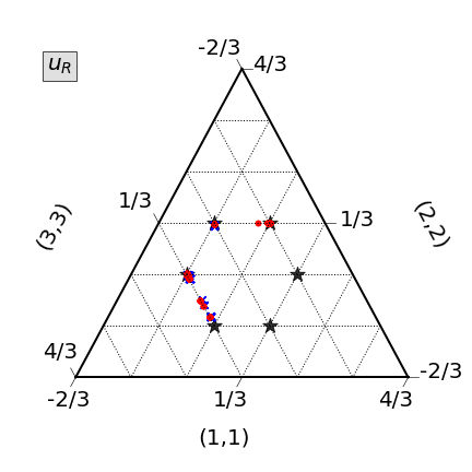
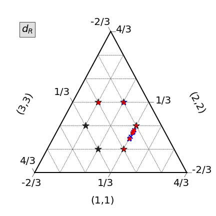
Refer to caption
Refer to caption
Figure 7: Preferred Uā€‹(1)ā€²š‘ˆsuperscript1ā€²U(1)^{\prime} charges in the mass basis for model M2, with x=1/3,y=0formulae-sequenceš‘„13š‘¦0x=1/3,\;y=0 and z=1š‘§1z=1.

For model M3a, there are two degenerate charges in all quark sectors. As such, there are three black stars in Fig.Ā 8 rather than six. Here, the right-handed up sector shows a significant deviation, while, for the down sector, the parameter points are practically on top of one of the black stars. Similar features can be found in model M3b but with the FCNCs being slightly subdued in the up sector and with some off-diagonal elements also in the down sector.
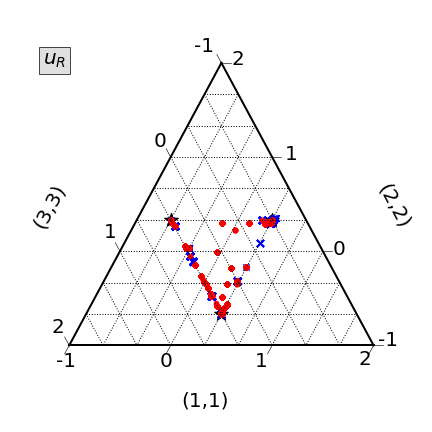
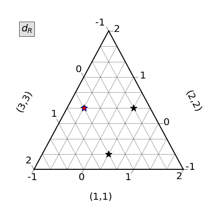
Refer to caption
Refer to caption
Figure 8: Preferred Uā€‹(1)ā€²š‘ˆsuperscript1ā€²U(1)^{\prime} charges in the mass basis for model M3a, with x=1/3,y=āˆ’2/3formulae-sequenceš‘„13š‘¦23x=1/3,\;y=-2/3 and z=1š‘§1z=1.

In Fig.Ā 9, we have the preferred Uā€‹(1)ā€²š‘ˆsuperscript1ā€²U(1)^{\prime} charges for model M7a. Here, there are sizable off-diagonal elements in both the right-handed sectors. For model M7b, the base-changing matrices are slightly closer to unity.
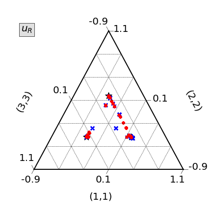
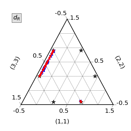
Refer to caption
Refer to caption
Figure 9: Preferred Uā€‹(1)ā€²š‘ˆsuperscript1ā€²U(1)^{\prime} charges in the mass basis for model M7a, with x=4/21š‘„421x=4/21 and y=āˆ’5/21š‘¦521y=-5/21.

Overall, we see that the ternary plots are dominated by red parameter points; i.e.Ā there is a strong preference toward a small Zāˆ’Zā€²š‘superscriptš‘ā€²Z-Z^{\prime} mixing.

V.3 Flavor anomalies

M2 M3a,b M4a M4b M5 M7a M7b
(1,2,3)123(1,2,3)\hskip 14.22636pt 0ā€‹(0)000\;(0)\hskip 28.45274pt 0ā€‹(0)000\;(0)\hskip 28.45274pt 0ā€‹(0)000\;(0)\hskip 28.45274pt 0ā€‹(āˆ’1322)013220\;\left(-\dfrac{13}{22}\right)\hskip 28.45274pt 0ā€‹(0)000\;(0)\hskip 28.45274pt 13āˆ—ā€‹(āˆž)āˆ—superscript13superscript\dfrac{1}{3}^{*}\;(\infty)^{*}\hskip 28.45274pt 0ā€‹(āˆ’112)01120\;\left(-\dfrac{11}{2}\right)
(1,3,2)132(1,3,2) 0ā€‹(0)000\;(0) 0ā€‹(0)000\;(0) 323ā€‹(0)3230\dfrac{3}{23}\;(0) 13āˆ—ā€‹(āˆž)āˆ—superscript13superscript\dfrac{1}{3}^{*}\;(\infty)^{*} 35ā€‹(0)350\dfrac{3}{5}\;(0) āˆ’3ā€‹(āˆ’10)310-3\;(-10) 13ā€‹(āˆž)āˆ—13superscript\dfrac{1}{3}\;(\infty)^{*}
(2,1,3)213(2,1,3) 13āˆ—ā€‹(āˆž)āˆ—superscript13superscript\dfrac{1}{3}^{*}\;(\infty)^{*} 13āˆ—ā€‹(āˆž)āˆ—superscript13superscript\dfrac{1}{3}^{*}\;(\infty)^{*} 13āˆ—ā€‹(āˆž)āˆ—superscript13superscript\dfrac{1}{3}^{*}\;(\infty)^{*} āˆ’313ā€‹(āˆ’2313)3132313-\dfrac{3}{13}\;\left(-\dfrac{23}{13}\right) 13āˆ—ā€‹(āˆž)āˆ—superscript13superscript\dfrac{1}{3}^{*}\;(\infty)^{*} 0ā€‹(0)000\;(0) 311ā€‹(āˆ’211)311211\dfrac{3}{11}\;\left(-\dfrac{2}{11}\right)
(2,3,1)231(2,3,1) 0ā€‹(āˆ’1)010\;(-1) 0ā€‹(āˆ’1)010\;(-1) 323ā€‹(āˆ’1423)3231423\dfrac{3}{23}\;\left(-\dfrac{14}{23}\right) 13āˆ—ā€‹(āˆž)āˆ—superscript13superscript\dfrac{1}{3}^{*}\;(\infty)^{*} 35ā€‹(45)3545\dfrac{3}{5}\;\left(\dfrac{4}{5}\right) āˆ’3ā€‹(0)30-3\;(0) 13āˆ—ā€‹(āˆž)āˆ—superscript13superscript\dfrac{1}{3}^{*}\;(\infty)^{*}
(3,1,2)312(3,1,2) 13ā€‹(āˆž)āˆ—13superscript\dfrac{1}{3}\;(\infty)^{*} 13āˆ—ā€‹(āˆž)āˆ—superscript13superscript\dfrac{1}{3}^{*}\;(\infty)^{*} 13āˆ—ā€‹(āˆž)āˆ—superscript13superscript\dfrac{1}{3}^{*}\;(\infty)^{*} āˆ’313ā€‹(0)3130-\dfrac{3}{13}\;(0) 13āˆ—ā€‹(āˆž)āˆ—superscript13superscript\dfrac{1}{3}^{*}\;(\infty)^{*} 0ā€‹(āˆ’110)01100\;\left(-\dfrac{1}{10}\right) 311ā€‹(0)3110\dfrac{3}{11}\;(0)
(3,2,1)321(3,2,1) 0ā€‹(āˆ’1)010\;(-1) 0ā€‹(āˆ’1)010\;(-1) 0ā€‹(āˆ’2314)023140\;\left(-\dfrac{23}{14}\right) 0ā€‹(0)000\;(0) 0ā€‹(54)0540\;\left(\dfrac{5}{4}\right) 13āˆ—ā€‹(āˆž)āˆ—superscript13superscript\dfrac{1}{3}^{*}\;(\infty)^{*} 0ā€‹(0)000\;(0)
Table 7: Values for C10NPā€‹Ī¼ā£(ā€²)/C9NPā€‹Ī¼ā£(ā€²)ā€‹(C9NPā€‹eā£(ā€²)/C9NPā€‹Ī¼ā£(ā€²))superscriptsubscriptš¶10NPšœ‡ā€²superscriptsubscriptš¶9NPšœ‡ā€²superscriptsubscriptš¶9NPš‘’ā€²superscriptsubscriptš¶9NPšœ‡ā€²{C_{10}^{\mathrm{NP}\mu(\prime)}}/{C_{9}^{\mathrm{NP}\mu(\prime)}}\;\left({C_{9}^{\mathrm{NP}e(\prime)}}/{C_{9}^{\mathrm{NP}\mu(\prime)}}\right). Here, the asterisk indicates entries for which C9NPā€‹Ī¼ā£(ā€²)superscriptsubscriptš¶9NPšœ‡ā€²C_{9}^{\mathrm{NP}\mu(\prime)} is zero, while shaded cells corresponds to the flavor configurations used in the scans.

The values for the ratios of C9,10NPā£(ā€²)superscriptsubscriptš¶910NPā€²C_{9,10}^{\mathrm{NP}(\prime)}, with the charge assignments in Eq.Ā (57), are shown in Table 7. Given these charges and the identification of the electron as the charged lepton with no Uā€‹(1)ā€²š‘ˆsuperscript1ā€²U(1)^{\prime} charge, the Wilson coefficients C9,10NPā€‹eā£(ā€²)superscriptsubscriptš¶910NPš‘’ā€²C_{9,10}^{\mathrm{NP}e(\prime)} are automatically zero for all models. It turns out that, for this choice, there is always a scenario where the muon couples vectorially to the Zā€²superscriptš‘ā€²Z^{\prime}, leaving C9NPā€‹Ī¼ā£(ā€²)superscriptsubscriptš¶9NPšœ‡ā€²C_{9}^{\mathrm{NP}\mu(\prime)} as the only nonzero Wilson coefficient. In Table 7, these cases are indicated by gray, shaded cells, which are also the scenarios used in the scan. Note that, for models M5 and M6b (and M1), the unprimed Wilson coefficients are zero, as there are no FCNCs in the left-handed down sector. Similarly, the primed Wilson coefficients are zero for models M6a and M6b (and M1), as they have no FCNCs in the right-handed down sector.

For most models, the predictions for RKsubscriptš‘…š¾R_{K} and RKāˆ—subscriptš‘…superscriptš¾āˆ—R_{K^{\ast}} were just the SM ones. However, for model M5, the presence of C9NPā€‹Ī¼ā£ā€²superscriptsubscriptš¶9NPšœ‡ā€²C_{9}^{\mathrm{NP}\mu\prime} was enough to have sizable deviations from the SM prediction. In Fig.Ā 10, we plot the ratio for RKāˆ—,RKsuperscriptsubscriptš‘…š¾subscriptš‘…š¾R_{K}^{*},R_{K} for model M5, together with the 1ā€‹Ļƒ1šœŽ1\sigma bounds for the LHCb and Belle measurements, as specified in Sec.Ā IV.2. Here we see that there are parameter points that can account for the current anomaly. Note that, in the plot, we are showing the values only in the region of interest for the anomaly - there exist plenty of points in agreement with the SM prediction and also with a larger value for RKsubscriptš‘…š¾R_{K} than 1.

Refer to caption
Figure 10: RKāˆ—superscriptsubscriptš‘…š¾R_{K}^{*} as a function of RKsubscriptš‘…š¾R_{K} for model M5, with the blue area indicating the 1ā€‹Ļƒ1šœŽ1\sigma LHCb bound, the orange area the Belle one, and where the SM value is indicated by a star.

We have also looked into the predictions of these models for the ratios RK,Kāˆ—Ī½subscriptsuperscriptš‘…šœˆš¾superscriptš¾āˆ—R^{\nu}_{K,K^{\ast}} as defined in Ref.Ā AltmannshoferĀ etĀ al. (2009). Most model predictions were compatible with the SM results. However, models M4a and M5 allowed some significant deviations. For model M4a (RKĪ½,RKāˆ—Ī½)superscriptsubscriptš‘…š¾šœˆsuperscriptsubscriptš‘…superscriptš¾āˆ—šœˆ(R_{K}^{\nu},R_{K^{\ast}}^{\nu}) varied from (0.8,1.1)0.81.1(0.8,1.1) to (1.3,0.85)1.30.85(1.3,0.85) linearly. In model M5, since there are only right-handed FCNCs, the two ratios are equal and were in the range [0.95,1.45]0.951.45[0.95,1.45].

VI Conclusions

This work has two central results. One is the classification of all anomaly-free 2HDMs with a gauged flavor symmetry, and the other is the analysis of their phenomenological consistency. Together, the two components can be used to identify the current research gap for this type of 2HDM and work as a starting point for further studies.

Out of the 116 model candidates corresponding to continuous symmetries in Ref.Ā FerreiraĀ andĀ Silva (2011), only 11 models survived after imposing anomaly cancellation. Six of these models were studied here for the first time. In the phenomenological study, each model was subjected to a range of observational constraints, and while there were good parameter points for all 11 models, we wish to give extra attention to models M2 and M5. For these two models, one could easily find extended regions of parameter space with a deviation below 3ā€‹Ļƒ3šœŽ3\sigma, in addition to model M5 being able to accommodate the RK,RKāˆ—subscriptš‘…š¾superscriptsubscriptš‘…š¾āˆ—R_{K},R_{K}^{\ast} anomaly with only the presence of C9NPā€‹Ī¼ā£ā€²superscriptsubscriptš¶9NPšœ‡ā€²C_{9}^{\mathrm{NP}\mu\prime}. As such, they deserve further consideration.

Acknowledgements.
The authors thank Johannes Bellm for enlightening discussions regarding collider bounds. H.S. also thanks JoĆ£o P. Silva for the careful reading and valuable comments on the manuscript. This work is supported in part by the Swedish Research Council, Contract No.Ā 2016-05996, and in part by the European Research Council (ERC) under the European Unionā€™s Horizon 2020 research and innovation program, Grant Agreement No.Ā 668679.

Appendix A Scalar potential

The scalar potential is given by V=V0+{V1+H.c.}V=V_{0}+\{V_{1}+\mathrm{H.c.}\}, where V0subscriptš‘‰0V_{0} is the phase-insensitive part

V0=āˆ‘i(mi2ā€‹|Ī¦i|2+Ī»iā€‹|Ī¦i|4)+Ī»12ā€‹|Ī¦1|2ā€‹|Ī¦2|2+Ī»12ā€²ā€‹|Ī¦1ā€ ā€‹Ī¦2|2+mS2ā€‹|S|2+Ī»Sā€‹|S|4+āˆ‘iĪ»Sā€‹iā€‹|Ī¦i|2ā€‹|S|2,subscriptš‘‰0subscriptš‘–superscriptsubscriptš‘šš‘–2superscriptsubscriptĪ¦š‘–2subscriptšœ†š‘–superscriptsubscriptĪ¦š‘–4subscriptšœ†12superscriptsubscriptĪ¦12superscriptsubscriptĪ¦22subscriptsuperscriptšœ†ā€²12superscriptsuperscriptsubscriptĪ¦1ā€ subscriptĪ¦22superscriptsubscriptš‘šš‘†2superscriptš‘†2subscriptšœ†š‘†superscriptš‘†4subscriptš‘–subscriptšœ†š‘†š‘–superscriptsubscriptĪ¦š‘–2superscriptš‘†2\displaystyle\begin{split}V_{0}&=\sum_{i}\left(m_{i}^{2}\left|\Phi_{i}\right|^{2}+\lambda_{i}\left|\Phi_{i}\right|^{4}\right)\\ &\;\;\;\;+\lambda_{12}\left|\Phi_{1}\right|^{2}\left|\Phi_{2}\right|^{2}+\lambda^{\prime}_{12}\left|\Phi_{1}^{\dagger}\Phi_{2}\right|^{2}\\ &\;\;\;\;+m_{S}^{2}\left|S\right|^{2}+\lambda_{S}\left|S\right|^{4}+\sum_{i}\lambda_{Si}\left|\Phi_{i}\right|^{2}\left|S\right|^{2},\end{split} (60)

with i=1,2š‘–12i=1,2, and V1subscriptš‘‰1V_{1} the phase-sensitive part

V1={a1ā€‹(2)ā€‹Ī¦1ā€ ā€‹Ī¦2ā€‹S(āˆ—)ā€‹forā€‹XS=+(āˆ’)(XĪ¦1āˆ’XĪ¦2)a3ā€‹(4)ā€‹Ī¦1ā€ ā€‹Ī¦2ā€‹S(āˆ—)2ā€‹forā€‹XS=+(āˆ’)(XĪ¦1āˆ’XĪ¦2)/2subscriptš‘‰1casessubscriptš‘Ž12superscriptsubscriptĪ¦1ā€ subscriptĪ¦2superscriptš‘†forsubscriptš‘‹š‘†fragments()subscriptš‘‹subscriptĪ¦1subscriptš‘‹subscriptĪ¦2otherwisesubscriptš‘Ž34superscriptsubscriptĪ¦1ā€ subscriptĪ¦2superscriptsuperscriptš‘†2forsubscriptš‘‹š‘†fragments()subscriptš‘‹subscriptĪ¦1subscriptš‘‹subscriptĪ¦22otherwise\displaystyle V_{1}=\begin{cases}a_{1(2)}\Phi_{1}^{\dagger}\Phi_{2}S^{(*)}\hskip 2.84526pt\mathrm{for}\hskip 1.42262ptX_{S}=\mathbin{\vbox{\hbox{\oalign{\hfil$\scriptstyle+$\hfil\cr\kern-2.15277pt\cr$\scriptscriptstyle({-})$\cr}}}}\left(X_{\Phi_{1}}-X_{\Phi_{2}}\right)\\[3.41432pt] a_{3(4)}\Phi_{1}^{\dagger}\Phi_{2}{S^{(*)}}^{2}\mathrm{for}\hskip 1.42262ptX_{S}=\mathbin{\vbox{\hbox{\oalign{\hfil$\scriptstyle+$\hfil\cr\kern-2.15277pt\cr$\scriptscriptstyle({-})$\cr}}}}(X_{\Phi_{1}}-X_{\Phi_{2}})/2\end{cases} (61)

where XĪ¦1,2subscriptš‘‹subscriptĪ¦12X_{\Phi_{1,2}} are the Uā€‹(1)ā€²š‘ˆsuperscript1ā€²U(1)^{\prime} charges of the Higgs doublets and XSsubscriptš‘‹š‘†X_{S} the Uā€‹(1)ā€²š‘ˆsuperscript1ā€²U(1)^{\prime} charge of the scalar singlet.

Note that only one of the four parameters in V1subscriptš‘‰1V_{1} can be nonzero at a time. As such, we can always choose all parameters to be real by a rephasing of the scalar singlet Sš‘†S, resulting in the scalar potential being Cā€‹Pš¶š‘ƒCP conserving. This, in turn, also inhibits the possibility of spontaneous Cā€‹Pš¶š‘ƒCP violation BrancoĀ andĀ Ivanov (2016).

Below, we present the complex tadpole equations. In expressions containing both a1ā€‹(2)subscriptš‘Ž12a_{1(2)} and a3ā€‹(4)subscriptš‘Ž34a_{3(4)} simultaneously, it is always implicit that only one of them can be present for each scalar potential variation. We then have

0ā‰”(MĀ±2)iā€‹jā€‹vj,0ā‰”(mS2+Ī»Sā€‹|vS|2+12ā€‹(Ī»Sā€‹1ā€‹v12+Ī»Sā€‹2ā€‹v22))ā€‹vSā€‹eiā€‹Ī±S+v1ā€‹v2ā€‹(a1ā€‹(2)2+a3ā€‹(4)ā€‹vSā€‹eāˆ’iā€‹Ī±S),formulae-sequence0subscriptsuperscriptsubscriptš‘€plus-or-minus2š‘–š‘—subscriptš‘£š‘—0superscriptsubscriptš‘šš‘†2subscriptšœ†š‘†superscriptsubscriptš‘£š‘†212subscriptšœ†š‘†1superscriptsubscriptš‘£12subscriptšœ†š‘†2superscriptsubscriptš‘£22subscriptš‘£š‘†superscriptš‘’š‘–subscriptš›¼š‘†subscriptš‘£1subscriptš‘£2subscriptš‘Ž122subscriptš‘Ž34subscriptš‘£š‘†superscriptš‘’š‘–subscriptš›¼š‘†\displaystyle\begin{split}0\equiv&\left(M_{\pm}^{2}\right)_{ij}v_{j}\,,\\ 0\equiv&\left(m_{S}^{2}+\lambda_{S}|v_{S}|^{2}+\frac{1}{2}(\lambda_{S1}v_{1}^{2}+\lambda_{S2}v_{2}^{2})\right)v_{S}e^{i\alpha_{S}}\\ &\quad+v_{1}v_{2}\left(\frac{a_{1(2)}}{\sqrt{2}}+a_{3(4)}v_{S}e^{-i\alpha_{S}}\right)\,,\end{split} (62)

with MĀ±2superscriptsubscriptš‘€plus-or-minus2M_{\pm}^{2} the Hermitian squared mass matrix for the charged scalars, defined as Ļ•aāˆ’ā€‹(MĀ±2)aā€‹bā€‹Ļ•b+superscriptsubscriptitalic-Ļ•š‘Žsubscriptsuperscriptsubscriptš‘€plus-or-minus2š‘Žš‘subscriptsuperscriptitalic-Ļ•š‘\phi_{a}^{-}\left(M_{\pm}^{2}\right)_{ab}\phi^{+}_{b} and given by

(MĀ±2)iā€‹i=mi2+Ī»iā€‹vi2+Ī»Sā€‹iā€²2ā€‹vS2+Ī»122ā€‹(v22ā€‹Ī“iā€‹1+v12ā€‹Ī“iā€‹2),(MĀ±2)12=Ī»12ā€²2ā€‹v2ā€‹v1+12ā€‹a1ā€‹(2)ā€‹vSā€‹e+(āˆ’)iā€‹Ī±S+12ā€‹a3ā€‹(4)ā€‹vS2ā€‹e+(āˆ’)iā€‹2ā€‹Ī±S.formulae-sequencesubscriptsuperscriptsubscriptš‘€plus-or-minus2š‘–š‘–superscriptsubscriptš‘šš‘–2subscriptšœ†š‘–superscriptsubscriptš‘£š‘–2superscriptsubscriptšœ†š‘†š‘–ā€²2superscriptsubscriptš‘£š‘†2subscriptšœ†122superscriptsubscriptš‘£22subscriptš›æš‘–1superscriptsubscriptš‘£12subscriptš›æš‘–2subscriptsuperscriptsubscriptš‘€plus-or-minus212subscriptsuperscriptšœ†ā€²122subscriptš‘£2subscriptš‘£112subscriptš‘Ž12subscriptš‘£š‘†superscriptš‘’fragments()š‘–subscriptš›¼š‘†12subscriptš‘Ž34superscriptsubscriptš‘£š‘†2superscriptš‘’fragments()š‘–2subscriptš›¼š‘†\displaystyle\begin{split}\left(M_{\pm}^{2}\right)_{ii}=&m_{i}^{2}+\lambda_{i}v_{i}^{2}+\frac{\lambda_{Si}^{\prime}}{2}v_{S}^{2}\\ &+\frac{\lambda_{12}}{2}(v_{2}^{2}\delta_{i1}+v_{1}^{2}\delta_{i2})\,,\\ \left(M_{\pm}^{2}\right)_{12}=&\frac{\lambda^{\prime}_{12}}{2}v_{2}v_{1}+\frac{1}{\sqrt{2}}a_{1(2)}v_{S}e^{\mathbin{\vbox{\hbox{\oalign{\hfil$\scriptstyle+$\hfil\cr\kern-1.50694pt\cr$\scriptscriptstyle({-})$\cr}}}}i\alpha_{S}}\\ &+\dfrac{1}{2}a_{3(4)}v_{S}^{2}e^{\mathbin{\vbox{\hbox{\oalign{\hfil$\scriptstyle+$\hfil\cr\kern-1.50694pt\cr$\scriptscriptstyle({-})$\cr}}}}i2\alpha_{S}}\,.\end{split} (63)

We can take the imaginary part of the tadpole equations and explicitly see that the phase of the singlet VEV can be only 0 or a multiple of Ļ€šœ‹\pi, for a1ā€‹(2)subscriptš‘Ž12a_{1(2)}, and multiple of Ļ€/2šœ‹2\pi/2, for a3ā€‹(4)subscriptš‘Ž34a_{3(4)}. From this point onwards, all expressions take the singlet phase to be zero. For the neutral scalars, the mass term is defined as

12ā€‹Ļ†0ā€‹Tā€‹M02ā€‹Ļ†0withĻ†0=(RaIaĻĪ·),12superscriptšœ‘0š‘‡superscriptsubscriptš‘€02superscriptšœ‘0withsuperscriptšœ‘0matrixsubscriptš‘…š‘Žsubscriptš¼š‘ŽšœŒšœ‚\displaystyle\begin{split}\frac{1}{2}\varphi^{0T}M_{0}^{2}\varphi^{0}\quad\text{with}\quad\varphi^{0}=\begin{pmatrix}R_{a}\\ I_{a}\\ \rho\\ \eta\end{pmatrix}\,,\end{split} (64)

following the notation used in Eq.Ā (1). Since Cā€‹Pš¶š‘ƒCP is conserved, there is no mixing between the Cā€‹Pš¶š‘ƒCP-even and Cā€‹Pš¶š‘ƒCP-odd scalar components, leading to the simplified symmetric neutral mass matrix

M02=(MRā€‹e2|Ļ•ā€‹Ļ•0MRā€‹e2|Ļ•ā€‹S0MIā€‹m2|Ļ•ā€‹Ļ•0MIā€‹m2|Ļ•ā€‹SMRā€‹e2|Sā€‹S0MIā€‹m2|Sā€‹S),M_{0}^{2}=\begin{pmatrix}\left.M_{Re}^{2}\right|^{\phi\phi}&0&\left.M_{Re}^{2}\right|^{\phi S}&0\\ &\left.M_{Im}^{2}\right|^{\phi\phi}&0&\left.M_{Im}^{2}\right|^{\phi S}\\ &&\left.M_{Re}^{2}\right|^{SS}&0\\ &&&\left.M_{Im}^{2}\right|^{SS}\end{pmatrix}\,, (65)

with the different entries explicitly given by

MRā€‹e2|Ļ•ā€‹Ļ•=MĀ±2+(2ā€‹Ī»1ā€‹v12+Ī»12ā€²2ā€‹v22(Ī»12+Ī»12ā€²2)ā€‹v1ā€‹v2(Ī»12+Ī»12ā€²2)ā€‹v1ā€‹v22ā€‹Ī»2ā€‹v22+Ī»12ā€²2ā€‹v12),MIā€‹m2|Ļ•ā€‹Ļ•=MĀ±2+12ā€‹Ī»12ā€²ā€‹(v22āˆ’v1ā€‹v2āˆ’v1ā€‹v2v12),MRā€‹e2|Sā€‹S=mS2+3ā€‹Ī»Sā€‹vS2+12ā€‹(Ī»Sā€‹1ā€‹v12+Ī»Sā€‹2ā€‹v22)+a3ā€‹(4)ā€‹v1ā€‹v2,MIā€‹m2|Sā€‹S=mS2+Ī»Sā€‹vS2+12ā€‹(Ī»Sā€‹1ā€‹v12+Ī»Sā€‹2ā€‹v22)āˆ’a3ā€‹(4)ā€‹v1ā€‹v2,\displaystyle\begin{split}\left.M_{Re}^{2}\right|^{\phi\phi}=&\;M_{\pm}^{2}+\begin{pmatrix}2\lambda_{1}v_{1}^{2}+\frac{\lambda_{12}^{\prime}}{2}v_{2}^{2}&(\lambda_{12}+\frac{\lambda_{12}^{\prime}}{2})v_{1}v_{2}\\ (\lambda_{12}+\frac{\lambda_{12}^{\prime}}{2})v_{1}v_{2}&2\lambda_{2}v_{2}^{2}+\frac{\lambda_{12}^{\prime}}{2}v_{1}^{2}\end{pmatrix}\,,\\ \left.M_{Im}^{2}\right|^{\phi\phi}=&\;M_{\pm}^{2}+\frac{1}{2}\lambda_{12}^{\prime}\begin{pmatrix}v_{2}^{2}&-v_{1}v_{2}\\ -v_{1}v_{2}&v_{1}^{2}\end{pmatrix}\,,\\ \left.M_{Re}^{2}\right|^{SS}=&\;m_{S}^{2}+3\lambda_{S}v_{S}^{2}+\frac{1}{2}(\lambda_{S1}v_{1}^{2}+\lambda_{S2}v_{2}^{2})\\ &+a_{3(4)}v_{1}v_{2}\,,\\ \left.M_{Im}^{2}\right|^{SS}=&\;m_{S}^{2}+\lambda_{S}v_{S}^{2}+\frac{1}{2}(\lambda_{S1}v_{1}^{2}+\lambda_{S2}v_{2}^{2})\\ &-a_{3(4)}v_{1}v_{2}\,,\end{split}
MRā€‹e2|Ļ•ā€‹S=(Ī»Sā€‹1ā€‹v1ā€‹vS+12ā€‹a1ā€‹(2)ā€‹v2+a3ā€‹(4)ā€‹vSā€‹v2Ī»Sā€‹2ā€‹v2ā€‹vS+12ā€‹a1ā€‹(2)ā€‹v1+a3ā€‹(4)ā€‹vSā€‹v1),MIā€‹m2|Ļ•ā€‹S=(12ā€‹a1ā€‹(2)ā€‹v2+a3ā€‹(4)ā€‹vSā€‹v2āˆ’12ā€‹a1ā€‹(2)ā€‹v1āˆ’a3ā€‹(4)ā€‹vSā€‹v1).\displaystyle\begin{split}\left.M_{Re}^{2}\right|^{\phi S}=&\begin{pmatrix}\lambda_{S1}v_{1}v_{S}+\frac{1}{\sqrt{2}}a_{1(2)}v_{2}+a_{3(4)}v_{S}v_{2}\\ \lambda_{S2}v_{2}v_{S}+\frac{1}{\sqrt{2}}a_{1(2)}v_{1}+a_{3(4)}v_{S}v_{1}\end{pmatrix}\,,\\ \left.M_{Im}^{2}\right|^{\phi S}=&\begin{pmatrix}\frac{1}{\sqrt{2}}a_{1(2)}v_{2}+a_{3(4)}v_{S}v_{2}\\ -\frac{1}{\sqrt{2}}a_{1(2)}v_{1}-a_{3(4)}v_{S}v_{1}\end{pmatrix}\,.\end{split}

Appendix B Anomaly conditions

There are six anomaly constraints involving Uā€‹(1)ā€²š‘ˆsuperscript1ā€²U(1)^{\prime} which does not cancel trivially, namely

A111ā€²=āˆ‘i=13(Xqi+3ā€‹Xā„“iāˆ’8ā€‹Xuiāˆ’2ā€‹Xdiāˆ’6ā€‹Xei),A11ā€²ā€‹1ā€²=āˆ‘i=13(Xqi2āˆ’Xā„“i2āˆ’2ā€‹Xui2+Xdi2+Xei2),A1ā€²ā€‹1ā€²ā€‹1ā€²=āˆ‘i=13(6ā€‹Xqi3+2ā€‹Xā„“i3āˆ’3ā€‹Xui3āˆ’3ā€‹Xdi3āˆ’Xei3),A221ā€²=āˆ‘i=13(3ā€‹Xqi+Xā„“i)A331ā€²=āˆ‘i=13(2ā€‹Xqiāˆ’Xuiāˆ’Xdi),Agā€‹gā€‹1ā€²=āˆ‘i=13(6ā€‹Xqi+2ā€‹Xā„“iāˆ’3ā€‹Xuiāˆ’3ā€‹Xdiāˆ’Xei),formulae-sequenceformulae-sequencesubscriptš“superscript111ā€²superscriptsubscriptš‘–13subscriptš‘‹subscriptš‘žš‘–3subscriptš‘‹subscriptā„“š‘–8subscriptš‘‹subscriptš‘¢š‘–2subscriptš‘‹subscriptš‘‘š‘–6subscriptš‘‹subscriptš‘’š‘–formulae-sequencesubscriptš“superscript11ā€²superscript1ā€²superscriptsubscriptš‘–13superscriptsubscriptš‘‹subscriptš‘žš‘–2superscriptsubscriptš‘‹subscriptā„“š‘–22superscriptsubscriptš‘‹subscriptš‘¢š‘–2superscriptsubscriptš‘‹subscriptš‘‘š‘–2superscriptsubscriptš‘‹subscriptš‘’š‘–2formulae-sequencesubscriptš“superscript1ā€²superscript1ā€²superscript1ā€²superscriptsubscriptš‘–136superscriptsubscriptš‘‹subscriptš‘žš‘–32superscriptsubscriptš‘‹subscriptā„“š‘–33superscriptsubscriptš‘‹subscriptš‘¢š‘–33superscriptsubscriptš‘‹subscriptš‘‘š‘–3superscriptsubscriptš‘‹subscriptš‘’š‘–3subscriptš“superscript221ā€²superscriptsubscriptš‘–133subscriptš‘‹subscriptš‘žš‘–subscriptš‘‹subscriptā„“š‘–subscriptš“superscript331ā€²superscriptsubscriptš‘–132subscriptš‘‹subscriptš‘žš‘–subscriptš‘‹subscriptš‘¢š‘–subscriptš‘‹subscriptš‘‘š‘–subscriptš“š‘”š‘”superscript1ā€²superscriptsubscriptš‘–136subscriptš‘‹subscriptš‘žš‘–2subscriptš‘‹subscriptā„“š‘–3subscriptš‘‹subscriptš‘¢š‘–3subscriptš‘‹subscriptš‘‘š‘–subscriptš‘‹subscriptš‘’š‘–\displaystyle\begin{split}A_{111^{\prime}}&=\sum_{i=1}^{3}\left(X_{q_{i}}+3X_{\ell_{i}}-8X_{u_{i}}-2X_{d_{i}}-6X_{e_{i}}\right),\\ A_{11^{\prime}1^{\prime}}&=\sum_{i=1}^{3}\left(X_{q_{i}}^{2}-X_{\ell_{i}}^{2}-2X_{u_{i}}^{2}+X_{d_{i}}^{2}+X_{e_{i}}^{2}\right),\\ A_{1^{\prime}1^{\prime}1^{\prime}}&=\sum_{i=1}^{3}\left(6X_{q_{i}}^{3}+2X_{\ell_{i}}^{3}-3X_{u_{i}}^{3}-3X_{d_{i}}^{3}-X_{e_{i}}^{3}\right),\\ A_{221^{\prime}}&=\sum_{i=1}^{3}\left(3X_{q_{i}}+X_{\ell_{i}}\right)\\ A_{331^{\prime}}&=\sum_{i=1}^{3}\left(2X_{q_{i}}-X_{u_{i}}-X_{d_{i}}\right),\\ A_{gg1^{\prime}}&=\sum_{i=1}^{3}\left(6X_{q_{i}}+2X_{\ell_{i}}-3X_{u_{i}}-3X_{d_{i}}-X_{e_{i}}\right),\end{split} (66)

where AXYZāˆTrā€‹({TX,TY}ā€‹TZ)proportional-tosubscriptš“XYZTrsubscriptš‘‡Xsubscriptš‘‡Ysubscriptš‘‡ZA_{\mathrm{XYZ}}\propto\mathrm{Tr}\left(\{T_{\mathrm{X}},T_{\mathrm{Y}}\}T_{\mathrm{Z}}\right), with TXsubscriptš‘‡XT_{\mathrm{X}} being a generator in the fundamental representation for the gauge group XX\mathrm{X}, and where Agā€‹gā€‹1ā€²subscriptš“š‘”š‘”superscript1ā€²A_{gg1^{\prime}} is the gravitational anomaly.

References

  • AadĀ etĀ al. (2012a) GeorgesĀ Aad etĀ al. (ATLAS),Ā ā€œObservation of a new particle in the search for the Standard Model Higgs boson with the ATLAS detector at the LHC,ā€Ā Phys. Lett.Ā B716,Ā 1ā€“29 (2012a),Ā arXiv:1207.7214 [hep-ex] .
  • ChatrchyanĀ etĀ al. (2012) SergueiĀ Chatrchyan etĀ al. (CMS),Ā ā€œObservation of a New Boson at a Mass of 125 GeV with the CMS Experiment at the LHC,ā€Ā Phys. Lett.Ā B716,Ā 30ā€“61 (2012),Ā arXiv:1207.7235 [hep-ex] .
  • BrancoĀ etĀ al. (2012) G.Ā C.Ā Branco, P.Ā M.Ā Ferreira, L.Ā Lavoura, M.Ā N.Ā Rebelo, MarcĀ Sher, Ā andĀ JoĆ£oĀ P.Ā Silva,Ā ā€œTheory and phenomenology of two-Higgs-doublet models,ā€Ā Phys. Rept.Ā 516,Ā 1ā€“102 (2012),Ā arXiv:1106.0034 [hep-ph] .
  • Ivanov (2017) IgorĀ P.Ā Ivanov,Ā ā€œBuilding and testing models with extended Higgs sectors,ā€Ā Prog. Part. Nucl. Phys.Ā 95,Ā 160ā€“208 (2017),Ā arXiv:1702.03776 [hep-ph] .
  • CrivellinĀ etĀ al. (2013) AndreasĀ Crivellin, AhmetĀ Kokulu, Ā andĀ ChristophĀ Greub,Ā ā€œFlavor-phenomenology of two-Higgs-doublet models with generic Yukawa structure,ā€Ā Phys. Rev.Ā D87,Ā 094031 (2013),Ā arXiv:1303.5877 [hep-ph] .
  • GlashowĀ andĀ Weinberg (1977) SheldonĀ GlashowĀ andĀ StevenĀ Weinberg,Ā ā€œNatural conservation laws for neutral currents,ā€Ā Phys. Rev. DĀ 15 (1977),Ā 10.1103/PhysRevD.15.1958.
  • Paschos (1977) EmmanuelĀ A.Ā Paschos,Ā ā€œDiagonal neutral currents,ā€Ā Phys. Rev. DĀ 15,Ā 1966ā€“1972 (1977).
  • BrancoĀ etĀ al. (1996) G.Ā C.Ā Branco, W.Ā Grimus, Ā andĀ L.Ā Lavoura,Ā ā€œRelating the scalar flavor changing neutral couplings to the CKM matrix,ā€Ā Phys. Lett.Ā B380,Ā 119ā€“126 (1996),Ā arXiv:hep-ph/9601383 [hep-ph] .
  • BurasĀ etĀ al. (2001) A.Ā J.Ā Buras, P.Ā Gambino, M.Ā Gorbahn, S.Ā Jager, Ā andĀ L.Ā Silvestrini,Ā ā€œUniversal unitarity triangle and physics beyond the standard model,ā€Ā Phys. Lett.Ā B500,Ā 161ā€“167 (2001),Ā arXiv:hep-ph/0007085 [hep-ph] .
  • Dā€™AmbrosioĀ etĀ al. (2002) G.Ā Dā€™Ambrosio, G.Ā F.Ā Giudice, G.Ā Isidori, Ā andĀ A.Ā Strumia,Ā ā€œMinimal flavor violation: An Effective field theory approach,ā€Ā Nucl. Phys.Ā B645,Ā 155ā€“187 (2002),Ā arXiv:hep-ph/0207036 [hep-ph] .
  • FerreiraĀ andĀ Silva (2011) P.Ā M.Ā FerreiraĀ andĀ JoĆ£oĀ P.Ā Silva,Ā ā€œAbelian symmetries in the two-Higgs-doublet model with fermions,ā€Ā Phys. Rev.Ā D83,Ā 065026 (2011),Ā arXiv:1012.2874 [hep-ph] .
  • SerĆ“dio (2013) H.Ā SerĆ“dio,Ā ā€œYukawa sector of Multi Higgs Doublet Models in the presence of Abelian symmetries,ā€Ā Phys. Rev.Ā D88,Ā 056015 (2013),Ā arXiv:1307.4773 [hep-ph] .
  • IvanovĀ andĀ Nishi (2013) I.Ā P.Ā IvanovĀ andĀ C.Ā C.Ā Nishi,Ā ā€œAbelian symmetries of the N-Higgs-doublet model with Yukawa interactions,ā€Ā JHEPĀ 11,Ā 069 (2013),Ā arXiv:1309.3682 [hep-ph] .
  • IvanovĀ etĀ al. (2012) IgorĀ P.Ā Ivanov, VenusĀ Keus, Ā andĀ EvgenyĀ Vdovin,Ā ā€œAbelian symmetries in multi-Higgs-doublet models,ā€Ā J. Phys.Ā A45,Ā 215201 (2012),Ā arXiv:1112.1660 [math-ph] .
  • DavidsonĀ etĀ al. (1979a) AharonĀ Davidson, MehmetĀ Koca, Ā andĀ KameshwarĀ C.Ā Wali,Ā ā€œU(1) as the Minimal Horizontal Gauge Symmetry,ā€Ā Phys. Rev. Lett.Ā 43,Ā 92 (1979a).
  • DavidsonĀ etĀ al. (1979b) AharonĀ Davidson, MehmetĀ Koca, Ā andĀ KameshwarĀ C.Ā Wali,Ā ā€œA Minimal Anomaly Free Electroweak Model for Several Generations,ā€Ā Phys. Rev.Ā D20,Ā 1195 (1979b).
  • DavidsonĀ andĀ Wali (1980) AharonĀ DavidsonĀ andĀ KameshwarĀ C.Ā Wali,Ā ā€œHorizontal-quantum-flavor-dynamics approach to the fermion mass spectrum,ā€Ā Phys. Rev.Ā D21,Ā 787 (1980).
  • Teichmann (2017) F.Ā Teichmann,Ā Abelian gauge symmetries in the two-Higgs-doublet model,Ā Masterā€™s thesis,Ā Lund University (2017).
  • TanabashiĀ etĀ al. (2018) M.Ā Tanabashi etĀ al. (Particle Data Group),Ā ā€œReview of Particle Physics,ā€Ā Phys. Rev.Ā D98,Ā 030001 (2018).
  • BabuĀ etĀ al. (1998) K.Ā S.Ā Babu, ChristopherĀ F.Ā Kolda, Ā andĀ JohnĀ March-Russell,Ā ā€œImplications of generalized Zāˆ’Zā€²š‘superscriptš‘ā€²Z-Z^{\prime} mixing,ā€Ā Phys. Rev.Ā D57,Ā 6788ā€“6792 (1998),Ā arXiv:hep-ph/9710441 [hep-ph] .
  • BatraĀ etĀ al. (2006) PuneetĀ Batra, BogdanĀ A.Ā Dobrescu, Ā andĀ DavidĀ Spivak,Ā ā€œAnomaly-free sets of fermions,ā€Ā J. Math. Phys.Ā 47,Ā 082301 (2006),Ā arXiv:hep-ph/0510181 [hep-ph] .
  • AllanachĀ etĀ al. (2019) B.Ā C.Ā Allanach, JoeĀ Davighi, Ā andĀ ScottĀ Melville,Ā ā€œAn Anomaly-free Atlas: charting the space of flavour-dependent gauged Uā€‹(1)š‘ˆ1U(1) extensions of the Standard Model,ā€Ā JHEPĀ 02,Ā 082 (2019),Ā [Erratum: JHEP08,064(2019)],Ā arXiv:1812.04602 [hep-ph] .
  • RathsmanĀ andĀ Tellander (2019) JohanĀ RathsmanĀ andĀ FelixĀ Tellander,Ā ā€œAnomaly-free Model Building with Algebraic Geometry,ā€Ā Ā  (2019),Ā arXiv:1902.08529 [hep-ph] .
  • CostaĀ etĀ al. (2019) DaviĀ B.Ā Costa, BogdanĀ A.Ā Dobrescu, Ā andĀ PatrickĀ J.Ā Fox,Ā ā€œGeneral solution to the U(1) anomaly equations,ā€Ā Ā (2019),Ā arXiv:1905.13729 [hep-th] .
  • GreenĀ andĀ Schwarz (1984) MichaelĀ B.Ā GreenĀ andĀ JohnĀ H.Ā Schwarz,Ā ā€œAnomaly Cancellation in Supersymmetric D=10 Gauge Theory and Superstring Theory,ā€Ā Phys. Lett.Ā 149B,Ā 117ā€“122 (1984).
  • GreenĀ andĀ Schwarz (1985) MichaelĀ B.Ā GreenĀ andĀ JohnĀ H.Ā Schwarz,Ā ā€œThe Hexagon Gauge Anomaly in Type I Superstring Theory,ā€Ā Nucl. Phys.Ā B255,Ā 93ā€“114 (1985).
  • GreenĀ etĀ al. (1985) MichaelĀ B.Ā Green, JohnĀ H.Ā Schwarz, Ā andĀ PeterĀ C.Ā West,Ā ā€œAnomaly Free Chiral Theories in Six-Dimensions,ā€Ā Nucl. Phys.Ā B254,Ā 327ā€“348 (1985).
  • Preskill (1991) JohnĀ Preskill,Ā ā€œGauge anomalies in an effective field theory,ā€Ā Annals Phys.Ā 210,Ā 323ā€“379 (1991).
  • CorianoĀ etĀ al. (2007) ClaudioĀ Coriano, NikosĀ Irges, Ā andĀ SimoneĀ Morelli,Ā ā€œStuckelberg axions and the effective action of anomalous Abelian models. 1. A Unitarity analysis of the Higgs-axion mixing,ā€Ā JHEPĀ 07,Ā 008 (2007),Ā arXiv:hep-ph/0701010 [hep-ph] .
  • IrgesĀ etĀ al. (2008) NikosĀ Irges, ClaudioĀ Coriano, Ā andĀ SimoneĀ Morelli,Ā ā€œStuckelberg Axions and the Effective Action of Anomalous Abelian Models 2. A SUā€‹(3)CƗSUā€‹(2)WƗUā€‹(1)YƗUā€‹(1)BSUsubscript3š¶SUsubscript2š‘ŠUsubscript1š‘ŒUsubscript1šµ\mathrm{SU}(3)_{C}\times\mathrm{SU}(2)_{W}\times\mathrm{U}(1)_{Y}\times\mathrm{U}(1)_{B} model and its signature at the LHC,ā€Ā Nucl. Phys.Ā B789,Ā 133ā€“174 (2008),Ā arXiv:hep-ph/0703127 [HEP-PH] .
  • EkstedtĀ etĀ al. (2018) AndreasĀ Ekstedt, RikardĀ Enberg, GunnarĀ Ingelman, JohanĀ Lƶfgren, Ā andĀ TanumoyĀ Mandal,Ā ā€œMinimal anomalous Uā€‹(1)U1\mathrm{U}(1) theories and collider phenomenology,ā€Ā JHEPĀ 02,Ā 152 (2018),Ā arXiv:1712.03410 [hep-ph] .
  • HaberĀ etĀ al. (1979) H.Ā E.Ā Haber, GordonĀ L.Ā Kane, Ā andĀ T.Ā Sterling,Ā ā€œThe Fermion Mass Scale and Possible Effects of Higgs Bosons on Experimental Observables,ā€Ā Nucl. Phys.Ā B161,Ā 493ā€“532 (1979).
  • CrivellinĀ etĀ al. (2015a) AndreasĀ Crivellin, GiancarloĀ Dā€™Ambrosio, Ā andĀ JulianĀ Heeck,Ā ā€œExplaining hā†’Ī¼Ā±ā€‹Ļ„āˆ“ā†’ā„Žsuperscriptšœ‡plus-or-minussuperscriptšœminus-or-plush\to\mu^{\pm}\tau^{\mp}, Bā†’Kāˆ—ā€‹Ī¼+ā€‹Ī¼āˆ’ā†’šµsuperscriptš¾superscriptšœ‡superscriptšœ‡B\to K^{*}\mu^{+}\mu^{-} and Bā†’Kā€‹Ī¼+ā€‹Ī¼āˆ’/Bā†’Kā€‹e+ā€‹eāˆ’ā†’šµš¾superscriptšœ‡superscriptšœ‡šµā†’š¾superscriptš‘’superscriptš‘’B\to K\mu^{+}\mu^{-}/B\to Ke^{+}e^{-} in a two-Higgs-doublet model with gauged LĪ¼āˆ’LĻ„subscriptšæšœ‡subscriptšæšœL_{\mu}-L_{\tau},ā€Ā Phys. Rev. Lett.Ā 114,Ā 151801 (2015a),Ā arXiv:1501.00993 [hep-ph] .
  • CamargoĀ etĀ al. (2019a) DanielĀ A.Ā Camargo, LuigiĀ DelleĀ Rose, StefanoĀ Moretti, Ā andĀ FarinaldoĀ S.Ā Queiroz,Ā ā€œCollider bounds on 2-Higgs doublet models with U(1)X gauge symmetries,ā€Ā Phys. Lett.Ā B793,Ā 150ā€“160 (2019a),Ā arXiv:1805.08231 [hep-ph] .
  • CamposĀ etĀ al. (2017) MiguelĀ D.Ā Campos, D.Ā Cogollo, ManfredĀ Lindner, T.Ā Melo, FarinaldoĀ S.Ā Queiroz, Ā andĀ WernerĀ Rodejohann,Ā ā€œNeutrino Masses and Absence of Flavor Changing Interactions in the 2HDM from Gauge Principles,ā€Ā JHEPĀ 08,Ā 092 (2017),Ā arXiv:1705.05388 [hep-ph] .
  • CamargoĀ etĀ al. (2019b) DanielĀ A.Ā Camargo, MiguelĀ D.Ā Campos, TessioĀ B.Ā deĀ Melo, Ā andĀ FarinaldoĀ S.Ā Queiroz,Ā ā€œA Two Higgs Doublet Model for Dark Matter and Neutrino Masses,ā€Ā Phys. Lett.Ā B795,Ā 319ā€“326 (2019b),Ā arXiv:1901.05476 [hep-ph] .
  • CelisĀ etĀ al. (2017) AlejandroĀ Celis, Wan-ZheĀ Feng, Ā andĀ MartinĀ Vollmann,Ā ā€œDirac dark matter and bā†’sā€‹ā„“+ā€‹ā„“āˆ’ā†’š‘š‘ superscriptā„“superscriptā„“b\to s\ell^{+}\ell^{-} with Uā€‹(1)U1\mathrm{U(1)} gauge symmetry,ā€Ā Phys. Rev.Ā D95,Ā 035018 (2017),Ā arXiv:1608.03894 [hep-ph] .
  • CrivellinĀ etĀ al. (2015b) AndreasĀ Crivellin, GiancarloĀ Dā€™Ambrosio, Ā andĀ JulianĀ Heeck,Ā ā€œAddressing the LHC flavor anomalies with horizontal gauge symmetries,ā€Ā Phys. Rev.Ā D91,Ā 075006 (2015b),Ā arXiv:1503.03477 [hep-ph] .
  • BianĀ etĀ al. (2018) LigongĀ Bian, HyunĀ MinĀ Lee, Ā andĀ ChanĀ BeomĀ Park,Ā ā€œBšµB-meson anomalies and Higgs physics in flavored Uā€‹(1)ā€²š‘ˆsuperscript1ā€²U(1)^{\prime} model,ā€Ā Eur. Phys. J.Ā C78,Ā 306 (2018),Ā arXiv:1711.08930 [hep-ph] .
  • BianĀ etĀ al. (2017) LigongĀ Bian, Soo-MinĀ Choi, Yoo-JinĀ Kang, Ā andĀ HyunĀ MinĀ Lee,Ā ā€œA minimal flavored Uā€‹(1)ā€²š‘ˆsuperscript1ā€²U(1)^{\prime} for BšµB-meson anomalies,ā€Ā Phys. Rev.Ā D96,Ā 075038 (2017),Ā arXiv:1707.04811 [hep-ph] .
  • KoĀ etĀ al. (2019) P.Ā Ko, TakaakiĀ Nomura, Ā andĀ ChaehyunĀ Yu,Ā ā€œbā†’sā€‹Ī¼+ā€‹Ī¼āˆ’ā†’š‘š‘ superscriptšœ‡superscriptšœ‡b\rightarrow s\mu^{+}\mu^{-} anomalies and related phenomenology in Uā€‹(1)B3āˆ’xĪ¼ā€‹LĪ¼āˆ’xĻ„ā€‹LĻ„š‘ˆsubscript1subscriptšµ3subscriptš‘„šœ‡subscriptšæšœ‡subscriptš‘„šœsubscriptšæšœU(1)_{B_{3}-x_{\mu}L_{\mu}-x_{\tau}L_{\tau}} flavor gauge models,ā€Ā JHEPĀ 04,Ā 102 (2019),Ā arXiv:1902.06107 [hep-ph] .
  • AlvesĀ etĀ al. (2018) JoĆ£oĀ M.Ā Alves, FranciscoĀ J.Ā Botella, GustavoĀ C.Ā Branco, FernandoĀ Cornet-Gomez, MiguelĀ Nebot, Ā andĀ JoĆ£oĀ P.Ā Silva,Ā ā€œSymmetry Constrained Two Higgs Doublet Models,ā€Ā Eur. Phys. J.Ā C78,Ā 630 (2018),Ā arXiv:1803.11199 [hep-ph] .
  • NomuraĀ andĀ Okada (2017) TakaakiĀ NomuraĀ andĀ HiroshiĀ Okada,Ā ā€œLoop suppressed light fermion masses with Uā€‹(1)Rš‘ˆsubscript1š‘…U(1)_{R} gauge symmetry,ā€Ā Phys. Rev.Ā D96,Ā 015016 (2017),Ā arXiv:1704.03382 [hep-ph] .
  • BotellaĀ etĀ al. (2014) F.Ā J.Ā Botella, G.Ā C.Ā Branco, AdrianĀ Carmona, M.Ā Nebot, LeonardoĀ Pedro, Ā andĀ M.Ā N.Ā Rebelo,Ā ā€œPhysical Constraints on a Class of Two-Higgs Doublet Models with FCNC at tree level,ā€Ā JHEPĀ 07,Ā 078 (2014),Ā arXiv:1401.6147 [hep-ph] .
  • CelisĀ etĀ al. (2015) AlejandroĀ Celis, JavierĀ Fuentes-Martin, MartĆ­nĀ Jung, Ā andĀ HugoĀ SerĆ“dio,Ā ā€œFamily nonuniversal Zā€²superscriptš‘ā€²Z^{\prime} models with protected flavor-changing interactions,ā€Ā Phys. Rev.Ā D92,Ā 015007 (2015),Ā arXiv:1505.03079 [hep-ph] .
  • GattoĀ etĀ al. (1980) RaoulĀ Gatto, G.Ā Morchio, G.Ā Sartori, Ā andĀ F.Ā Strocchi,Ā ā€œNatural Flavor Conservation in Higgs Induced Neutral Currents and the Quark Mixing Angles,ā€Ā Nucl. Phys.Ā B163,Ā 221ā€“253 (1980).
  • NovikovĀ etĀ al. (1995a) V.Ā Novikov, L.Ā Okun, Ā andĀ M.Ā Vysotsky,Ā ā€œā€™LEPTOPā€™: Electroweak corrections at LEP-1,ā€Ā Surveys in high energy physics. Proceedings, 22nd ITEP Winter School, Polyani, Zvenigorod, Russia, February 22-March 2, 1994,Ā Surveys High Energ. Phys.Ā 8,Ā 81ā€“90 (1995a).
  • NovikovĀ etĀ al. (1995b) V.Ā Novikov, L.Ā Okun, AlexandreĀ N.Ā Rozanov, Ā andĀ M.Ā Vysotsky,Ā ā€œLEPTOP,ā€Ā Ā  (1995b),Ā arXiv:hep-ph/9503308 [hep-ph] .
  • GrimusĀ etĀ al. (2008) W.Ā Grimus, L.Ā Lavoura, O.Ā M.Ā Ogreid, Ā andĀ P.Ā Osland,Ā ā€œThe Oblique parameters in multi-Higgs-doublet models,ā€Ā Nucl. Phys.Ā B801,Ā 81ā€“96 (2008),Ā arXiv:0802.4353 [hep-ph] .
  • BurgessĀ etĀ al. (1994) C.Ā P.Ā Burgess, StephenĀ Godfrey, HeinzĀ Konig, DavidĀ London, Ā andĀ IvanĀ Maksymyk,Ā ā€œModel independent global constraints on new physics,ā€Ā Phys. Rev.Ā D49,Ā 6115ā€“6147 (1994),Ā arXiv:hep-ph/9312291 [hep-ph] .
  • SchaelĀ etĀ al. (2013) S.Ā Schael etĀ al. (ALEPH, DELPHI, L3, OPAL, LEP Electroweak),Ā ā€œElectroweak Measurements in Electron-Positron Collisions at W-Boson-Pair Energies at LEP,ā€Ā Phys. Rept.Ā 532,Ā 119ā€“244 (2013),Ā arXiv:1302.3415 [hep-ex] .
  • ErlerĀ etĀ al. (2003) JensĀ Erler, AndriyĀ Kurylov, Ā andĀ MichaelĀ JĀ Ramsey-Musolf,Ā ā€œThe Weak charge of the proton and new physics,ā€Ā Phys. Rev.Ā D68,Ā 016006 (2003),Ā arXiv:hep-ph/0302149 [hep-ph] .
  • GingesĀ andĀ Flambaum (2004) J.Ā S.Ā M.Ā GingesĀ andĀ V.Ā V.Ā Flambaum,Ā ā€œViolations of fundamental symmetries in atoms and tests of unification theories of elementary particles,ā€Ā Phys. Rept.Ā 397,Ā 63ā€“154 (2004),Ā arXiv:physics/0309054 [physics] .
  • JungĀ andĀ Pich (2014) MartinĀ JungĀ andĀ AntonioĀ Pich,Ā ā€œElectric Dipole Moments in Two-Higgs-Doublet Models,ā€Ā JHEPĀ 04,Ā 076 (2014),Ā arXiv:1308.6283 [hep-ph] .
  • BarrĀ andĀ Zee (1990) StephenĀ M.Ā BarrĀ andĀ A.Ā Zee,Ā ā€œElectric Dipole Moment of the Electron and of the Neutron,ā€Ā Phys. Rev. Lett.Ā 65,Ā 21ā€“24 (1990),Ā [Erratum: Phys. Rev. Lett.65,2920(1990)].
  • AbeĀ etĀ al. (2014) TomohiroĀ Abe, JunjiĀ Hisano, TeppeiĀ Kitahara, Ā andĀ KohsakuĀ Tobioka,Ā ā€œGauge invariant Barr-Zee type contributions to fermionic EDMs in the two-Higgs doublet models,ā€Ā JHEPĀ 01,Ā 106 (2014),Ā [Erratum: JHEP04,161(2016)],Ā arXiv:1311.4704 [hep-ph] .
  • JegerlehnerĀ andĀ Nyffeler (2009) FredĀ JegerlehnerĀ andĀ AndreasĀ Nyffeler,Ā ā€œThe Muon g-2,ā€Ā Phys. Rept.Ā 477,Ā 1ā€“110 (2009),Ā arXiv:0902.3360 [hep-ph] .
  • BurasĀ etĀ al. (2013a) AndrzejĀ J.Ā Buras, FulviaĀ DeĀ Fazio, Ā andĀ JenniferĀ Girrbach,Ā ā€œThe Anatomy of Zā€™ and Z with Flavour Changing Neutral Currents in the Flavour Precision Era,ā€Ā JHEPĀ 02,Ā 116 (2013a),Ā arXiv:1211.1896 [hep-ph] .
  • BurasĀ etĀ al. (2013b) AndrzejĀ J.Ā Buras, FulviaĀ DeĀ Fazio, JenniferĀ Girrbach, RobertĀ Knegjens, Ā andĀ MinoruĀ Nagai,Ā ā€œThe Anatomy of Neutral Scalars with FCNCs in the Flavour Precision Era,ā€Ā JHEPĀ 06,Ā 111 (2013b),Ā arXiv:1303.3723 [hep-ph] .
  • BurasĀ etĀ al. (2014) AndrzejĀ J.Ā Buras, DarioĀ Buttazzo, JenniferĀ Girrbach-Noe, Ā andĀ RobertĀ Knegjens,Ā ā€œCan we reach the Zeptouniverse with rare K and Bs,dsubscriptšµš‘ š‘‘B_{s,d} decays?ā€Ā JHEPĀ 11,Ā 121 (2014),Ā arXiv:1408.0728 [hep-ph] .
  • GolowichĀ etĀ al. (2007) EugeneĀ Golowich, JoAnneĀ Hewett, SandipĀ Pakvasa, Ā andĀ AlexeyĀ A.Ā Petrov,Ā ā€œImplications of D0superscriptš·0D^{0} - DĀÆ0superscriptĀÆš·0\bar{D}^{0} Mixing for New Physics,ā€Ā Phys. Rev.Ā D76,Ā 095009 (2007),Ā arXiv:0705.3650 [hep-ph] .
  • GolowichĀ etĀ al. (2009) EugeneĀ Golowich, JoAnneĀ Hewett, SandipĀ Pakvasa, Ā andĀ AlexeyĀ A.Ā Petrov,Ā ā€œRelating D0superscriptš·0D^{0} - DĀÆ0superscriptĀÆš·0\bar{D}^{0} Mixing and D0ā†’l+ā€‹lāˆ’ā†’superscriptš·0superscriptš‘™superscriptš‘™D^{0}\rightarrow l^{+}l^{-} with New Physics,ā€Ā Phys. Rev.Ā D79,Ā 114030 (2009),Ā arXiv:0903.2830 [hep-ph] .
  • BurasĀ etĀ al. (2012) AndrzejĀ J.Ā Buras, JenniferĀ Girrbach, DiegoĀ Guadagnoli, Ā andĀ GinoĀ Isidori,Ā ā€œOn the Standard Model prediction for BR(Bs,dā†’Ī¼+ā€‹Ī¼āˆ’ā†’subscriptšµš‘ š‘‘superscriptšœ‡superscriptšœ‡B_{s,d}\rightarrow\mu^{+}\mu^{-}),ā€Ā Eur. Phys. J.Ā C72,Ā 2172 (2012),Ā arXiv:1208.0934 [hep-ph] .
  • BurasĀ etĀ al. (2013c) AndrzejĀ J.Ā Buras, RobertĀ Fleischer, JenniferĀ Girrbach, Ā andĀ RobertĀ Knegjens,Ā ā€œProbing New Physics with the Bssubscriptšµš‘ B_{s} to Ī¼+ā€‹Ī¼āˆ’superscriptšœ‡superscriptšœ‡{\mu}^{+}{\mu}^{-} Time-Dependent Rate,ā€Ā JHEPĀ 07,Ā 77 (2013c),Ā arXiv:1303.3820 [hep-ph] .
  • DeĀ BruynĀ etĀ al. (2012) KristofĀ DeĀ Bruyn, RobertĀ Fleischer, RobertĀ Knegjens, PatrickĀ Koppenburg, MarcelĀ Merk, Ā andĀ NielsĀ Tuning,Ā ā€œBranching Ratio Measurements of Bssubscriptšµš‘ B_{s} Decays,ā€Ā Phys. Rev.Ā D86,Ā 014027 (2012),Ā arXiv:1204.1735 [hep-ph] .
  • AaijĀ etĀ al. (2017a) RoelĀ Aaij etĀ al. (LHCb),Ā ā€œMeasurement of the Bs0ā†’Ī¼+ā€‹Ī¼āˆ’ā†’subscriptsuperscriptšµ0š‘ superscriptšœ‡superscriptšœ‡B^{0}_{s}\to\mu^{+}\mu^{-} branching fraction and effective lifetime and search for B0ā†’Ī¼+ā€‹Ī¼āˆ’ā†’superscriptšµ0superscriptšœ‡superscriptšœ‡B^{0}\to\mu^{+}\mu^{-} decays,ā€Ā Phys. Rev. Lett.Ā 118,Ā 191801 (2017a),Ā arXiv:1703.05747 [hep-ex] .
  • MisiakĀ etĀ al. (2015) M.Ā Misiak etĀ al.,Ā ā€œUpdated NNLO QCD predictions for the weak radiative B-meson decays,ā€Ā Phys. Rev. Lett.Ā 114,Ā 221801 (2015),Ā arXiv:1503.01789 [hep-ph] .
  • BurasĀ etĀ al. (2011) AndrzejĀ J.Ā Buras, LucaĀ Merlo, Ā andĀ EmmanuelĀ Stamou,Ā ā€œThe Impact of Flavour Changing Neutral Gauge Bosons on BĀÆā†’Xsā€‹Ī³ā†’ĀÆšµsubscriptš‘‹š‘ š›¾\bar{B}\rightarrow X_{s}\gamma,ā€Ā JHEPĀ 08,Ā 124 (2011),Ā arXiv:1105.5146 [hep-ph] .
  • EckerĀ andĀ Pich (1991) G.Ā EckerĀ andĀ A.Ā Pich,Ā ā€œThe Longitudinal muon polarization in KLā†’ā†’subscriptš¾Labsent{K}_{\mathrm{L}}\rightarrow Ī¼+ā€‹Ī¼āˆ’superscriptšœ‡superscriptšœ‡\mu^{+}\mu^{-},ā€Ā Nucl. Phys.Ā B366,Ā 189ā€“205 (1991).
  • IsidoriĀ andĀ Unterdorfer (2004) GinoĀ IsidoriĀ andĀ ReneĀ Unterdorfer,Ā ā€œOn the short distance constraints from KL,Sā†’Ī¼+ā€‹Ī¼āˆ’ā†’subscriptš¾šæš‘†superscriptšœ‡superscriptšœ‡K_{L,S}\rightarrow\mu^{+}\mu^{-},ā€Ā JHEPĀ 01,Ā 009 (2004),Ā arXiv:hep-ph/0311084 [hep-ph] .
  • Dā€™AmbrosioĀ andĀ Kitahara (2017) GiancarloĀ Dā€™AmbrosioĀ andĀ TeppeiĀ Kitahara,Ā ā€œDirect Cā€‹Pš¶š‘ƒCP Violation in Kā†’Ī¼+ā€‹Ī¼āˆ’ā†’š¾superscriptšœ‡superscriptšœ‡K\to\mu^{+}\mu^{-},ā€Ā Phys. Rev. Lett.Ā 119,Ā 201802 (2017),Ā arXiv:1707.06999 [hep-ph] .
  • AaijĀ etĀ al. (2017b) RoelĀ Aaij etĀ al. (LHCb),Ā ā€œImproved limit on the branching fraction of the rare decay KS0ā†’Ī¼+ā€‹Ī¼āˆ’ā†’subscriptsuperscriptš¾0Ssuperscriptšœ‡superscriptšœ‡{{K}^{0}_{\mathrm{\scriptscriptstyle S}}}\rightarrow\mu^{+}\mu^{-},ā€Ā Eur. Phys. J.Ā C77,Ā 678 (2017b),Ā arXiv:1706.00758 [hep-ex] .
  • ArtamonovĀ etĀ al. (2008) A.Ā V.Ā Artamonov etĀ al. (E949),Ā ā€œNew measurement of the K+ā†’Ļ€+ā€‹Ī½ā€‹Ī½ĀÆā†’superscriptš¾superscriptšœ‹šœˆĀÆšœˆK^{+}\to\pi^{+}\nu\bar{\nu} branching ratio,ā€Ā Phys. Rev. Lett.Ā 101,Ā 191802 (2008),Ā arXiv:0808.2459 [hep-ex] .
  • BobethĀ etĀ al. (2017) ChristophĀ Bobeth, AndrzejĀ J.Ā Buras, AlejandroĀ Celis, Ā andĀ MartinĀ Jung,Ā ā€œPatterns of Flavour Violation in Models with Vector-Like Quarks,ā€Ā JHEPĀ 04,Ā 079 (2017),Ā arXiv:1609.04783 [hep-ph] .
  • BurasĀ etĀ al. (2015) AndrzejĀ J.Ā Buras, DarioĀ Buttazzo, JenniferĀ Girrbach-Noe, Ā andĀ RobertĀ Knegjens,Ā ā€œK+ā†’Ļ€+ā€‹Ī½ā€‹Ī½ĀÆā†’superscriptš¾superscriptšœ‹šœˆĀÆšœˆ{K}^{+}\to{\pi}^{+}\nu\overline{\nu} and KLā†’Ļ€0ā€‹Ī½ā€‹Ī½ĀÆā†’subscriptš¾šæsuperscriptšœ‹0šœˆĀÆšœˆ{K}_{L}\to{\pi}^{0}\nu\overline{\nu} in the Standard Model: status and perspectives,ā€Ā JHEPĀ 11,Ā 033 (2015),Ā arXiv:1503.02693 [hep-ph] .
  • MesciaĀ etĀ al. (2006) FedericoĀ Mescia, ChristopherĀ Smith, Ā andĀ StephanieĀ Trine,Ā ā€œKLā†’Ļ€0ā€‹e+ā€‹eāˆ’ā†’subscriptš¾šæsuperscriptšœ‹0superscriptš‘’superscriptš‘’K_{L}\rightarrow\pi^{0}e^{+}e^{-} and KLā†’Ļ€0ā€‹Ī¼+ā€‹Ī¼āˆ’ā†’subscriptš¾šæsuperscriptšœ‹0superscriptšœ‡superscriptšœ‡K_{L}\rightarrow\pi^{0}\mu^{+}\mu^{-}: A Binary star on the stage of flavor physics,ā€Ā JHEPĀ 08,Ā 088 (2006),Ā arXiv:hep-ph/0606081 [hep-ph] .
  • BlankeĀ etĀ al. (2007) MonikaĀ Blanke, AndrzejĀ J.Ā Buras, AntonĀ Poschenrieder, StefanĀ Recksiegel, CeciliaĀ Tarantino, SelmaĀ Uhlig, Ā andĀ AndreasĀ Weiler,Ā ā€œRare and CP-Violating Kš¾K and BšµB Decays in the Littlest Higgs Model with Tāˆ’superscriptš‘‡T^{-} Parity,ā€Ā JHEPĀ 01,Ā 066 (2007),Ā arXiv:hep-ph/0610298 [hep-ph] .
  • BuchallaĀ etĀ al. (2003) GerhardĀ Buchalla, GiancarloĀ Dā€™Ambrosio, Ā andĀ GinoĀ Isidori,Ā ā€œExtracting short distance physics from KL,Sā†’Ļ€0ā€‹e+ā€‹eāˆ’ā†’subscriptš¾šæš‘†superscriptšœ‹0superscriptš‘’superscriptš‘’K_{L,S}\rightarrow\pi^{0}e^{+}e^{-} decays,ā€Ā Nucl. Phys.Ā B672,Ā 387ā€“408 (2003),Ā arXiv:hep-ph/0308008 [hep-ph] .
  • Alavi-HaratiĀ etĀ al. (2004) A.Ā Alavi-Harati etĀ al. (KTeV),Ā ā€œSearch for the rare decay KLā†’Ļ€0ā€‹e+ā€‹eāˆ’ā†’subscriptš¾šæsuperscriptšœ‹0superscriptš‘’superscriptš‘’K_{L}\rightarrow\pi^{0}e^{+}e^{-},ā€Ā Phys. Rev. Lett.Ā 93,Ā 021805 (2004),Ā arXiv:hep-ex/0309072 [hep-ex] .
  • Alavi-HaratiĀ etĀ al. (2000) A.Ā Alavi-Harati etĀ al. (KTEV),Ā ā€œSearch for the Decay KLā†’Ļ€0ā€‹Ī¼+ā€‹Ī¼āˆ’ā†’subscriptš¾šæsuperscriptšœ‹0superscriptšœ‡superscriptšœ‡K_{L}\to\pi^{0}\mu^{+}\mu^{-},ā€Ā Phys. Rev. Lett.Ā 84,Ā 5279ā€“5282 (2000),Ā arXiv:hep-ex/0001006 [hep-ex] .
  • AaijĀ etĀ al. (2014) RoelĀ Aaij etĀ al. (LHCb),Ā ā€œTest of lepton universality using B+ā†’K+ā€‹ā„“+ā€‹ā„“āˆ’ā†’superscriptšµsuperscriptš¾superscriptā„“superscriptā„“B^{+}\rightarrow K^{+}\ell^{+}\ell^{-} decays,ā€Ā Phys. Rev. Lett.Ā 113,Ā 151601 (2014),Ā arXiv:1406.6482 [hep-ex] .
  • Descotes-GenonĀ etĀ al. (2013) SebastienĀ Descotes-Genon, JoaquimĀ Matias, Ā andĀ JavierĀ Virto,Ā ā€œUnderstanding the Bā†’Kāˆ—ā€‹Ī¼+ā€‹Ī¼āˆ’ā†’šµsuperscriptš¾superscriptšœ‡superscriptšœ‡B\to K^{*}\mu^{+}\mu^{-} Anomaly,ā€Ā Phys. Rev.Ā D88,Ā 074002 (2013),Ā arXiv:1307.5683 [hep-ph] .
  • AltmannshoferĀ andĀ Straub (2013) WolfgangĀ AltmannshoferĀ andĀ DavidĀ M.Ā Straub,Ā ā€œNew Physics in Bā†’Kāˆ—ā€‹Ī¼ā€‹Ī¼ā†’šµsuperscriptš¾šœ‡šœ‡B\to K^{*}\mu\mu?ā€Ā Eur. Phys. J.Ā C73,Ā 2646 (2013),Ā arXiv:1308.1501 [hep-ph] .
  • AltmannshoferĀ andĀ Straub (2015) WolfgangĀ AltmannshoferĀ andĀ DavidĀ M.Ā Straub,Ā ā€œNew physics in bā†’sā†’š‘š‘ b\rightarrow s transitions after LHC run 1,ā€Ā Eur. Phys. J.Ā C75,Ā 382 (2015),Ā arXiv:1411.3161 [hep-ph] .
  • AlguerĆ³Ā etĀ al. (2019) MarcelĀ AlguerĆ³, BernatĀ Capdevila, AndreasĀ Crivellin, SĆ©bastienĀ Descotes-Genon, PereĀ Masjuan, JoaquimĀ Matias, Ā andĀ JavierĀ Virto,Ā ā€œEmerging patterns of New Physics with and without Lepton Flavour Universal contributions,ā€Ā Eur. Phys. J.Ā C79,Ā 714 (2019),Ā arXiv:1903.09578 [hep-ph] .
  • AaijĀ etĀ al. (2019) RoelĀ Aaij etĀ al. (LHCb),Ā ā€œSearch for lepton-universality violation in B+ā†’K+ā€‹ā„“+ā€‹ā„“āˆ’ā†’superscriptšµsuperscriptš¾superscriptā„“superscriptā„“B^{+}\to K^{+}\ell^{+}\ell^{-} decays,ā€Ā Phys. Rev. Lett.Ā 122,Ā 191801 (2019),Ā arXiv:1903.09252 [hep-ex] .
  • HillerĀ andĀ Kruger (2004) GudrunĀ HillerĀ andĀ FrankĀ Kruger,Ā ā€œMore model-independent analysis of bā†’sā†’š‘š‘ b\to s processes,ā€Ā Phys. Rev.Ā D69,Ā 074020 (2004),Ā arXiv:hep-ph/0310219 [hep-ph] .
  • AbdesselamĀ etĀ al. (2019a) A.Ā Abdesselam etĀ al. (Belle),Ā ā€œTest of lepton flavor universality in Bā†’Kā€‹ā„“+ā€‹ā„“āˆ’ā†’šµš¾superscriptā„“superscriptā„“B\to K\ell^{+}\ell^{-} decays,ā€Ā  (2019a),Ā arXiv:1908.01848 [hep-ex] .
  • AbdesselamĀ etĀ al. (2019b) A.Ā Abdesselam etĀ al. (Belle),Ā ā€œTest of lepton flavor universality in Bā†’Kāˆ—ā€‹ā„“+ā€‹ā„“āˆ’ā†’šµsuperscriptš¾āˆ—superscriptā„“superscriptā„“{B\to K^{\ast}\ell^{+}\ell^{-}} decays at Belle,ā€Ā Ā  (2019b),Ā arXiv:1904.02440 [hep-ex] .
  • HillerĀ andĀ Schmaltz (2015) GudrunĀ HillerĀ andĀ MartinĀ Schmaltz,Ā ā€œDiagnosing lepton-nonuniversality in bā†’sā€‹ā„“ā€‹ā„“ā†’š‘š‘ ā„“ā„“b\to s\ell\ell,ā€Ā JHEPĀ 02,Ā 055 (2015),Ā arXiv:1411.4773 [hep-ph] .
  • AltmannshoferĀ etĀ al. (2009) WolfgangĀ Altmannshofer, AndrzejĀ J.Ā Buras, DavidĀ M.Ā Straub, Ā andĀ MichaelĀ Wick,Ā ā€œNew strategies for New Physics search in Bā†’Kāˆ—ā€‹Ī½ā€‹Ī½ĀÆā†’šµsuperscriptš¾šœˆĀÆšœˆB\to K^{*}\nu\bar{\nu}, Bā†’Kā€‹Ī½ā€‹Ī½ĀÆā†’šµš¾šœˆĀÆšœˆB\to K\nu\bar{\nu} and Bā†’Xsā€‹Ī½ā€‹Ī½ĀÆā†’šµsubscriptš‘‹š‘ šœˆĀÆšœˆB\to X_{s}\nu\bar{\nu} decays,ā€Ā JHEPĀ 04,Ā 022 (2009),Ā arXiv:0902.0160 [hep-ph] .
  • BarateĀ etĀ al. (2001) R.Ā Barate etĀ al. (ALEPH),Ā ā€œMeasurements of BR(bā†’Ļ„āˆ’ā€‹Ī½ĀÆĻ„ā€‹Xā†’š‘superscriptšœsubscriptĀÆšœˆšœš‘‹b\rightarrow\tau^{-}\bar{\nu}_{\tau}X) and BR(bā†’Ļ„āˆ’ā€‹Ī½ĀÆĻ„ā€‹Dāˆ—Ā±ā€‹Xā†’š‘superscriptšœsubscriptĀÆšœˆšœsuperscriptš·āˆ—absentplus-or-minusš‘‹b\rightarrow\tau^{-}\bar{\nu}_{\tau}D^{\ast\pm}X) and upper limits on BR(Bāˆ’ā†’Ļ„āˆ’ā€‹Ī½ĀÆĻ„ā†’superscriptšµsuperscriptšœsubscriptĀÆšœˆšœB^{-}\rightarrow\tau^{-}\bar{\nu}_{\tau}) and BR(bā†’sā€‹Ī½ā€‹Ī½ĀÆā†’š‘š‘ šœˆĀÆšœˆb\rightarrow s\nu\bar{\nu}),ā€Ā Eur. Phys. J.Ā C19,Ā 213ā€“227 (2001),Ā arXiv:hep-ex/0010022 [hep-ex] .
  • ChenĀ etĀ al. (2007) K.Ā F.Ā Chen etĀ al. (Belle),Ā ā€œSearch for Bā†’h(āˆ—)ā€‹Ī½ā€‹Ī½ĀÆā†’šµsuperscriptā„ŽšœˆĀÆšœˆB\to h^{(*)}\nu\bar{\nu} decays at Belle,ā€Ā Phys. Rev. Lett.Ā 99,Ā 221802 (2007),Ā arXiv:0707.0138 [hep-ex] .
  • AubertĀ etĀ al. (2008) BernardĀ Aubert etĀ al. (BaBar),Ā ā€œSearch for Bā†’Kāˆ—ā€‹Ī½ā€‹Ī½ĀÆā†’šµsuperscriptš¾šœˆĀÆšœˆB\to K^{*}\nu\bar{\nu} decays,ā€Ā Phys. Rev.Ā D78,Ā 072007 (2008),Ā arXiv:0808.1338 [hep-ex] .
  • CarenaĀ etĀ al. (2004) MarcelaĀ Carena, AlejandroĀ Daleo, BogdanĀ A.Ā Dobrescu, Ā andĀ Timothy M.Ā P.Ā Tait,Ā ā€œZā€²superscriptš‘ā€²Z^{\prime} gauge bosons at the Tevatron,ā€Ā Phys. Rev.Ā D70,Ā 093009 (2004),Ā arXiv:hep-ph/0408098 [hep-ph] .
  • AccomandoĀ etĀ al. (2011) ElenaĀ Accomando, AlexanderĀ Belyaev, LucaĀ Fedeli, StephenĀ F.Ā King, Ā andĀ ClaireĀ Shepherd-Themistocleous,Ā ā€œZā€™ physics with early LHC data,ā€Ā Phys. Rev.Ā D83,Ā 075012 (2011),Ā arXiv:1010.6058 [hep-ph] .
  • PazĀ andĀ Roy (2018) GilĀ PazĀ andĀ JoydeepĀ Roy,Ā ā€œRemarks on the Zā€²superscriptš‘ā€²Z^{\prime} Drell-Yan cross section,ā€Ā Phys. Rev.Ā D97,Ā 075025 (2018),Ā arXiv:1711.02655 [hep-ph] .
  • BallĀ etĀ al. (2013) RichardĀ D.Ā Ball, ValerioĀ Bertone, StefanoĀ Carrazza, LuigiĀ DelĀ Debbio, StefanoĀ Forte, AlbertoĀ Guffanti, NathanĀ P.Ā Hartland, Ā andĀ JuanĀ Rojo (NNPDF),Ā ā€œParton distributions with QED corrections,ā€Ā Nucl. Phys.Ā B877,Ā 290ā€“320 (2013),Ā arXiv:1308.0598 [hep-ph] .
  • AadĀ etĀ al. (2019) GeorgesĀ Aad etĀ al. (ATLAS),Ā ā€œSearch for high-mass dilepton resonances using 139 fb-1 of pā€‹pš‘š‘pp collision data collected at s=š‘ absent\sqrt{s}= 13 TeV with the ATLAS detector,ā€Ā Phys. Lett.Ā B796,Ā 68ā€“87 (2019),Ā arXiv:1903.06248 [hep-ex] .
  • AadĀ etĀ al. (2014) GeorgesĀ Aad etĀ al. (ATLAS),Ā ā€œSearch for high-mass dilepton resonances in pp collisions at s=8š‘ 8\sqrt{s}=8 TeV with the ATLAS detector,ā€Ā Phys. Rev.Ā D90,Ā 052005 (2014),Ā arXiv:1405.4123 [hep-ex] .
  • AadĀ etĀ al. (2012b) GeorgesĀ Aad etĀ al. (ATLAS),Ā ā€œSearch for high-mass resonances decaying to dilepton final states in pp collisions at s=š‘ absent\sqrt{s}= 7 TeV with the ATLAS detector,ā€Ā JHEPĀ 11,Ā 138 (2012b),Ā arXiv:1209.2535 [hep-ex] .
  • AaboudĀ etĀ al. (2018a) MoradĀ Aaboud etĀ al. (ATLAS),Ā ā€œSearch for additional heavy neutral Higgs and gauge bosons in the ditau final state produced in 36 fbāˆ’1 of pp collisions at s=13š‘ 13\sqrt{s}=13 TeV with the ATLAS detector,ā€Ā JHEPĀ 01,Ā 055 (2018a),Ā arXiv:1709.07242 [hep-ex] .
  • AadĀ etĀ al. (2015) GeorgesĀ Aad etĀ al. (ATLAS),Ā ā€œA search for high-mass resonances decaying to Ļ„+ā€‹Ļ„āˆ’superscriptšœsuperscriptšœ\tau^{+}\tau^{-} in pā€‹pš‘š‘pp collisions at s=8š‘ 8\sqrt{s}=8 TeV with the ATLAS detector,ā€Ā JHEPĀ 07,Ā 157 (2015),Ā arXiv:1502.07177 [hep-ex] .
  • AaboudĀ etĀ al. (2019) MoradĀ Aaboud etĀ al. (ATLAS),Ā ā€œSearch for heavy particles decaying into a top-quark pair in the fully hadronic final state in pā€‹pš‘š‘pp collisions at s=š‘ absent\sqrt{s}= 13 TeV with the ATLAS detector,ā€Ā Phys. Rev.Ā D99,Ā 092004 (2019),Ā arXiv:1902.10077 [hep-ex] .
  • AaboudĀ etĀ al. (2018b) MoradĀ Aaboud etĀ al. (ATLAS),Ā ā€œSearch for heavy particles decaying into top-quark pairs using lepton-plus-jets events in proton-proton collisions at s=13š‘ 13\sqrt{s}=13 TeV with the ATLAS detector,ā€Ā Eur. Phys. J.Ā C78,Ā 565 (2018b),Ā arXiv:1804.10823 [hep-ex] .
  • Collaboration (2017) CMSĀ Collaboration (CMS),Ā ā€œSearches for dijet resonances in pp collisions at s=13ā€‹TeVš‘ 13TeV\sqrt{s}=13\leavevmode\nobreak\ \mathrm{TeV} using data collected in 2016.ā€Ā Ā  (2017).
  • SirunyanĀ etĀ al. (2018a) AlbertĀ MĀ Sirunyan etĀ al. (CMS),Ā ā€œSearch for massive resonances decaying into Wā€‹Wš‘Šš‘ŠWW, Wā€‹Zš‘Šš‘WZ, Zā€‹Zš‘š‘ZZ, qā€‹Wš‘žš‘ŠqW, and qā€‹Zš‘žš‘qZ with dijet final states at s=13ā€‹Ā Ā ā€‹TeVš‘ 13Ā Ā TeV\sqrt{s}=13\text{ }\text{ }\mathrm{TeV},ā€Ā Phys. Rev.Ā D97,Ā 072006 (2018a),Ā arXiv:1708.05379 [hep-ex] .
  • SirunyanĀ etĀ al. (2017) AlbertĀ MĀ Sirunyan etĀ al. (CMS),Ā ā€œSearch for massive resonances decaying into WW, WZ or ZZ bosons in proton-proton collisions at s=š‘ absent\sqrt{s}= 13 TeV,ā€Ā JHEPĀ 03,Ā 162 (2017),Ā arXiv:1612.09159 [hep-ex] .
  • AaboudĀ etĀ al. (2018c) MoradĀ Aaboud etĀ al. (ATLAS),Ā ā€œSearch for Wā€‹W/Wā€‹Zš‘Šš‘Šš‘Šš‘WW/WZ resonance production in ā„“ā€‹Ī½ā€‹qā€‹qā„“šœˆš‘žš‘ž\ell\nu qq final states in pā€‹pš‘š‘pp collisions at s=š‘ absent\sqrt{s}= 13 TeV with the ATLAS detector,ā€Ā JHEPĀ 03,Ā 042 (2018c),Ā arXiv:1710.07235 [hep-ex] .
  • collaboration (2017) TheĀ ATLASĀ collaboration (ATLAS),Ā ā€œSearch for heavy resonances decaying to a Wš‘ŠW or Zš‘Z boson and a Higgs boson in final states with leptons and bš‘b-jets in 36.1Ā fb-1 of pā€‹pš‘š‘pp collision data at s=13š‘ 13\sqrt{s}=13Ā TeV with the ATLAS detector,ā€Ā Ā  (2017).
  • SirunyanĀ etĀ al. (2018b) AlbertĀ MĀ Sirunyan etĀ al. (CMS),Ā ā€œSearch for ZĪ³š›¾\gamma resonances using leptonic and hadronic final states in proton-proton collisions at s=š‘ absent\sqrt{s}= 13 TeV,ā€Ā JHEPĀ 09,Ā 148 (2018b),Ā arXiv:1712.03143 [hep-ex] .
  • BrancoĀ andĀ Ivanov (2016) G.Ā C.Ā BrancoĀ andĀ I.Ā P.Ā Ivanov,Ā ā€œGroup-theoretic restrictions on generation of CP-violation in multi-Higgs-doublet models,ā€Ā JHEPĀ 01,Ā 116 (2016),Ā arXiv:1511.02764 [hep-ph] .