Tasks in Modular Proofs
of Concurrent Algorithms

Abstract

Proving correctness of distributed or concurrent algorithms is a mind-challenging and complex process. Slight errors in the reasoning are difficult to find, calling for computer-checked proof systems. In order to build computer-checked proofs with usual tools, such as Coq or TLA⁺, having sequential specifications of all base objects that are used as building blocks in a given algorithm is a requisite to provide a modular proof built by composition. Alas, many concurrent objects do not have a sequential specification.

This article describes a systematic method to transform any task, a specification method that captures concurrent one-shot distributed problems, into a sequential specification involving two calls, $\mathsf{set}$ and $\mathsf{get}$. This transformation allows system designers to compose proofs, thus providing a framework for modular computer-checked proofs of algorithms designed using tasks and sequential objects as building blocks. The Moir&Anderson implementation of renaming using splitters is an iconic example of such algorithms designed by composition.

Keywords: Formal methods $\cdot$ Verification $\cdot$ Concurrent algorithms $\cdot$ Renaming.

1 Introduction

Fault-tolerant distributed and concurrent algorithms are extensively used in critical systems that require strict guarantees of correctness [23]; consequently, verifying such algorithms is becoming more important nowadays. Yet, proving distributed and concurrent algorithms is a difficult and error-prone task, due to the complex interleavings that may occur in an execution. Therefore, it is crucial to develop frameworks that help assessing the correctness of such systems.

A major breakthrough in the direction of systematic proofs of concurrent algorithms is the notion of atomic or linearizable objects [20]: a linearizable object behaves as if it is accessed sequentially, even in presence of concurrent invocations, the canonical example being the atomic register. Atomicity lets us model a concurrent algorithm as a transition system in which each transition corresponds to an atomic step performed by a process on a base object. Human beings naturally reason on sequences of events happening one after the other; concurrency and interleavings seem to be more difficult to deal with.

However, it is well understood now that several natural one-shot base objects used in concurrent algorithms cannot be expressed as sequential objects [9, 16, 33] providing a single operation.

An iconic example is the splitter abstraction [31], which is the basis of the classical Moir&Anderson renaming algorithm [31]. Intuitively, a splitter is a concurrent one-shot problem that splits calling processes as follows: whenever $p$ processes access a splitter, at most one process obtains $\mathsf{stop}$, at most $p-1$ obtain $\mathsf{right}$ and at most $p-1$ obtain $\mathsf{down}$. Moir&Anderson renaming algorithm uses splitters arranged in a half grid to scatter processes and provide new names to processes. It is worth to mention that, since its introduction almost thirty years ago, the renaming problem [4] has become a paradigm for studying symmetry-breaking in concurrent systems (see, for example, [1, 8]).

A second example is the exchanger object provided in Java, which has been used for implementing efficient linearizable elimination stacks [16, 24, 36]. Roughly speaking, an exchanger is a meeting point where pairs of processes can exchange values, with the constraint that an exchange can happen only if the two processes run concurrently.

Splitters and exchangers are instances of one-shot concurrent objects known in the literature as tasks. Tasks have played a fundamental role in understanding the computability power of several models, providing a topological view of concurrent and distributed computing [18]. Intuitively, a task is an object providing a single one-shot operation, formally specified through an input domain, an output domain and an input/output relation describing the valid output configurations when a set of processes run concurrently, starting from a given input configuration. Tasks can be equivalently specified by mappings between topological objects: an input simplicial complex (i.e., a discretization of a continuous topological space) modeling all possible input assignments, an output simplicial complex modeling all possible output assignments, and a carrier map relating inputs and outputs.

Contributions.

Our main contribution is a generic transformation of any task $T$ (with a single operation) into a sequential object $S$ providing two operations, $\mathsf{set}$ and $\mathsf{get}$. The behavior of $S$ “mimics” the one of $T$ by splitting each invocation of a process to $T$ into two invocations to $S$, first $\mathsf{set}$ and then $\mathsf{get}$. Intuitively, the $\mathsf{set}$ operation records the processes that are participating to the execution of the task. A process actually calls the task and obtains a return value by invoking $\mathsf{get}$. Each of the operations is atomic; however, $\mathsf{set}$ and $\mathsf{get}$ invocations of a given process may be interleaved with similar invocations from other processes.

We show that these two operations are sufficient for any task, no matter how complicated it may be; since a task is a mapping between simplicial complexes, it can specify very complex concurrent behaviors, sometimes with obscure associated operational semantics.

A main benefit of our transformation is that one can replace an object solving a task $T$ by its associated sequential object $S$, and reason as if all steps happen sequentially. This allows us to obtain simpler models of concurrent algorithms using solutions to tasks and sequential objects as building blocks, leading to modular correctness proofs. Concretely, we can obtain a simple transition system of Moir&Anderson renaming algorithm, which helps to reason about it. In a companion paper [22], our model is used to derive a full and modular TLA⁺ proof of the algorithm, the first available TLA⁺ proof of it.

In Section 2, we explain the ideas in Moir&Anderson renaming algorithm that motivated our general transformation, which is presented in Section 3. Due to lack of space, some basic definitions, proofs and detailed constructions are omitted. They can be found in the extended version [7].

2 Verifying Moir&Anderson Renaming

We consider a concurrent system with $n$ asynchronous processes, meaning that each process can experience arbitrarily long delays during an execution. Moreover, processes may crash at any time, i.e., permanently stopping taking steps. Each process is associated with a unique $\mbox{\rm ID}\in\mathbb{N}$. The processes can access base objects like simple atomic read/write registers or more complex objects.

The original Moir&Anderson renaming algorithm [31] is designed and explained with splitters. Their seminal work first introduces the splitter algorithm based on atomic read/write registers and discusses its properties. Then, they describe a renaming algorithm that uses a grid of splitters. The actual implementation inlines splitters into the code of the renaming algorithm, and their proof is performed on the resulting program that uses solely read/write registers as base objects.

The Splitter Abstraction.

A splitter [31] is a one-shot concurrent task in which each process starts with its unique $\mbox{\rm ID}\in\mathbb{N}$ and has to return a value satisfying the following properties: (1) ${\sf Validity}$. The returned value is $\mathsf{right}$, $\mathsf{down}$  or $\mathsf{stop}$. (2) ${\sf Splitting}$. If $p\geq 1$ processes participate in an execution of the splitter, then at most $p-1$ processes obtain the value $\mathsf{right}$, at most $p-1$ processes obtain the value $\mathsf{down}$, at most one process obtains the value $\mathsf{stop}$. (3) ${\sf Termination}$. Every correct process (which doesn’t crash) returns a value.

Notice that if a process runs solo, i.e., $p=1$, it must obtain $\mathsf{stop}$, since the $\mathsf{splitting}$ property holds for any $p\geq 1$.

initially $\mathit{CLOSED}=false$ operation $\mathsf{splitter}()$: (01) $\mathit{LAST}\leftarrow my\_ID$; (02) if $(\mathit{CLOSED})$ (03) then $\mathsf{return}(\mathsf{right})$ (04) else $\mathit{CLOSED}\leftarrow\mathit{true}$; (05) if ($\mathit{LAST}=my\_ID$) (06) then ${\mathsf{return}}(\mathsf{stop})$ (07) else ${\mathsf{return}}(\mathsf{down})$ (08) end if (09) end if.

Figure 1: Implementation of a Splitter [31].

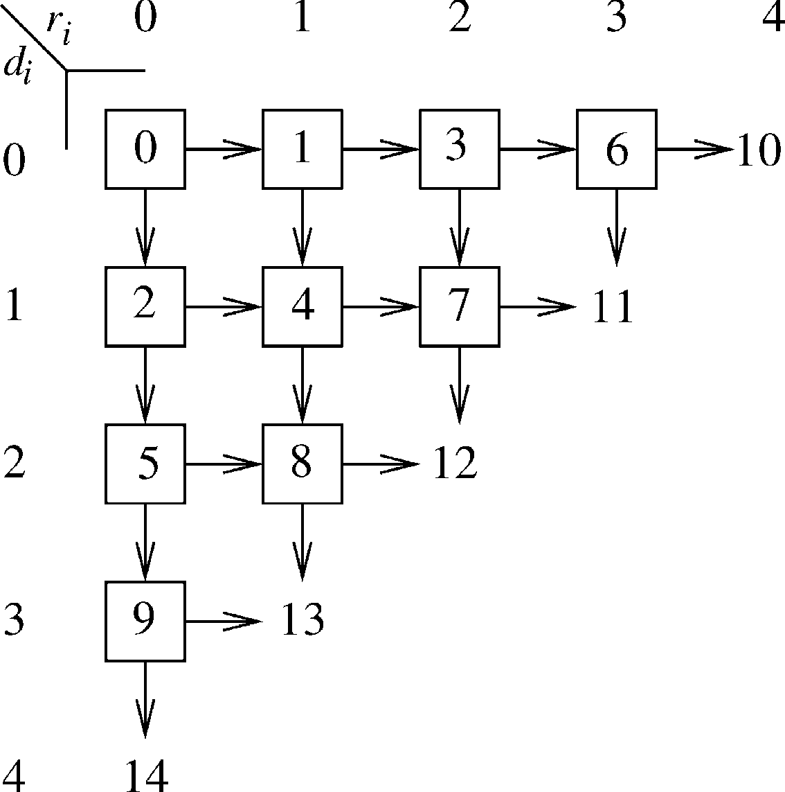
Figure 2: Renaming using Splitters.

Figure 2 contains the simple and elegant splitter implementation based on atomic read/write registers from [31] (register names have been changed for clarity). After carefully analyzing the code, the reader can convince herself that the algorithm described in Figure 2 implements the splitter specification. The fact that the implementation is based on atomic registers allows us to obtain a transition system of it in which each transition corresponds to an atomic operation on an object. The benefit of this modelization is that every execution of the implementation is simply described as a sequence of steps, as concurrent and distributed systems are usually modeled (see, for example, [19, 35])). Although the splitter implementation is very short and simple, its TLA⁺ proof is long and rather complex —particularly when considering that it uses a boolean register and a plain register only— (see [22] for details).

The Renaming Problem.

In the $M$-renaming task [4], each process starts with its unique $\mbox{\rm ID}\in\mathbb{N}$, and processes are required to return an output name satisfying the following properties: (1) ${\sf Validity}$. The output name of a process belongs to $[1,\ldots,M]$. (2) ${\sf Uniqueness}$. No two processes obtain the same output name. (3) ${\sf Termination}$. Every correct process returns an output name.

Let $p$ be the number of processes that participate in a given renaming instance. A renaming implementation is adaptive if the size $M$ of the new name space depends only on $p$, the number of participating processes. We have then $M=f(p)$ where $f(p)$ is a function on $p$ such that $f(1)=1$ and, for $2\leq p\leq n$, $p-1\leq f(p-1)\leq f(p)$.

Moir&Anderson Splitter-Based Renaming Algorithm.

Moir and Anderson propose in [31] a read/write renaming algorithm designed using the splitter abstraction. The algorithm is conceptually simple: for up to $n$ processes, a set of $n(n+1)/2$ splitters are placed in a half-grid, each with a unique name, as shown in Figure 2 for $n=5$. Each process starts invoking the splitter at the top-left corner, following the directions obtained at each splitter. When a splitter invocation returns stop, the process returns the name associated with the splitter. We use here an adaptive version of their algorithm that allows $p$ participating processes to rename in at most $p(p+1)/2$ names; the original solution in [31] is non-adaptive and the only difference is the labelling of the splitters in the grid.

Splitters as Sequential Objects?

Although Moir&Anderson renaming algorithm is easily described in a modular way, the actual program is not modular as each splitter in the conceptual grid is replaced by an independent copy of the splitter implementation of Figure 2. Thus, the correctness proof in [31] deals with the possible interleavings that can occur, considering all read/write splitter implementations in the grid.

In the light of the simple splitter based conceptual description, we would like to have a transition system describing the algorithm based on splitters as building blocks, in which each step corresponds to a splitter invocation. Such a description would be very beneficial as it would allow us to obtain a modular correctness proof showing that the algorithm is correct as long as the building blocks are splitters, hence the correctness is independent of any particular splitter implementation.

State: Sets $Participants,Stop,Down,Right$
all sets are initialized to $\emptyset$
Function $\mathsf{set}$(id)
	Pre-condition: $\mbox{\rm id}\notin Participants$
	Post-condition: $Participants^{\prime}\leftarrow Participants\cup\{\mbox{\rm id}\}$
	Output: $\sf void$
endFunction
Function $\mathsf{get}$(id)
	Pre-condition: $\mbox{\rm id}\in Participants\wedge\mbox{\rm id}\notin Stop,Down,Right$
	Post-condition:
		$D\leftarrow\emptyset$
		if $|Stop|=0$ then $D\leftarrow D\cup\{\mathsf{stop}\}$
		if $|Down|<|Participants|-1$ then $D\leftarrow D\cup\{\mathsf{down}\}$
		if $|Right|<|Participants|-1$ then $D\leftarrow D\cup\{\mathsf{right}\}$
		Let $dec$ be any value in $D$
		if $dec=$ $\mathsf{stop}$ then $Stop\leftarrow Stop\cup\{\mbox{\rm id}\}$
		if $dec=$ $\mathsf{down}$ then $Down\leftarrow Down\cup\{\mbox{\rm id}\}$
		if $dec=$ $\mathsf{right}$ then $Right\leftarrow Right\cup\{\mbox{\rm id}\}$
	Output: $dec$
endFunction

Figure 3: An ad hoc specification of the Splitter.

As it is formally proved in Section 3, it is impossible to obtain such a transition system. The obstacle is that a splitter is inherently concurrent and cannot be specified as a sequential object with a single operation. The intuition of the impossibility is the following. By contradiction, suppose that there is a sequential object corresponding to a splitter. Since the object is sequential, in every execution, the object behaves as if it is accessed sequentially (even in presence of concurrent invocation). Then, there is always a process that invokes the splitter object first, which, as noted above, must obtain $\mathsf{stop}$. The rest of the processes can obtain either $\mathsf{down}$ or $\mathsf{right}$, without any restriction (the value obtained by the first process precludes that all obtain $\mathsf{right}$ or all $\mathsf{down}$). However, such an object is allowing strictly fewer behaviors: in the original splitter definition it is perfectly possible that all processes run concurrently and half of them obtain $\mathsf{right}$ and the other half obtain $\mathsf{down}$, while none obtains $\mathsf{stop}$.

The splitter task as a sequential object.

One can circumvent the impossibility described above by splitting the single method provided by a splitter into two (atomic) operations of a sequential object. Figure 3 presents a sequential specification of a splitter with two operations, $\mathsf{set}$ and $\mathsf{get}$, using a standard pre/post-condition specification style. Each process invoking the splitter, first invokes $\mathsf{set}$ and then $\mathsf{get}$ (always in that order). The idea is that the $\mathsf{set}$ operation first records in the state of the object the processes that are participating in the splitter, so far, and then the $\mathsf{get}$ operation nondeterministically produces an output to a process, considering the rules of the splitter. In Section 3, we formally prove that this sequential object indeed models the splitter defined above.

Proving Moir&Anderson Renaming with Splitters as Base Sequential Objects.

Using the sequential specification of a splitter in Figure 3, we can easily obtain a generic description of the original Moir&Anderson splitter-based algorithm: each renaming object is replaced with an equivalent sequential version of it, and every process accessing a renaming object asynchronously invokes first $\mathsf{set}$ and then $\mathsf{get}$, which returns a direction to the process. The resulting algorithm does not rely on any particular splitter implementation, and uses only atomic objects, which allows us to obtain a transition system of it. This is the algorithm that is verified in TLA⁺ in [22]. The equivalence between the concurrent renaming specification and the sequential $\mathsf{set}$/$\mathsf{get}$ specification imply that the proof in [22] also proves for the original Moir&Anderson splitter-based algorithm.

3 Dealing with Tasks without Sequential Specification

In this section, we show that the transformation in Section 2 of the splitter task into a sequential object with two operations, $\mathsf{get}$ and $\mathsf{set}$, is not a trick but rather a general methodology to deal with tasks without a sequential specification. Our $\mathsf{get}$/$\mathsf{set}$ solution proposed here is reminiscent to the request-follow-up transformation in [25] that allows to transform a partial method of a sequential object (e.g. a queue with a blocking dequeue method when the queue is empty) into two total methods: a total request method registering that a process wants to obtain an output, and a total follow-up method obtaining the output value, or false if the conditions for obtaining a value are not yet satisfied (the process invokes the follow-up method until it gets an output). We stress that the request-follow-up transformation [25] considers only objects with a sequential specification and is not shown to be general as it is only used for queues and stacks.

Model of Computation in Detail.

We consider a standard concurrent system with $n$ asynchronous processes, $p_{1},\ldots,p_{n}$, which may crash at any time during an execution of the system, i.e., stopping taking steps (for more detail see for example [19, 35]). Processes communicate with each other by invoking operations on shared, concurrent base objects. A base object can provide ${\sf Read}/{\sf Write}$ operations (also called register), more powerful operations, such as ${\sf Test\&Set},{\sf Fetch\&Add},{\sf Swap}\textrm{~{}or~{}}{\sf Compare\&Swap}$, or solve a concurrent distributed problem, for example, $\mathsf{Splitter}$, $\mathsf{Renaming}$ or $\mathsf{Set\_Agreement}$.

Each process follows a local state machines $A_{1},\ldots,A_{n}$, where $A_{i}$ specifies which operations on base objects $p_{i}$ executes in order to return a response when it invokes a high-level operation (e.g. $\mathsf{push}$ or $\mathsf{pop}$ operations). Each of these base-objects operation invocations is a step. An execution is a possibly infinite sequence of steps and invocations and responses of high-level operations, with the following properties:

1. Each process first invokes a high-level operation, and only when it has a corresponding response, it can invoke another high-level operation, i.e., executions are well-formed.

2. For any invocation $inv(\langle\mathsf{opType},p_{i},input\rangle)$ of a process $p_{i}$, the steps of $p_{i}$ between that invocation and its corresponding response (if there is one), are steps that are specified by $A_{i}$ when $p_{i}$ invokes the high-level operation $\langle\mathsf{opType},p_{i},input\rangle$.

A high-level operation in an execution is complete if both its invocation and response appear in the execution. An operation is pending if only its invocation appears in the execution. A process is correct in an execution if it takes infinitely many steps.

Sequential Specifications.

A central paradigm for specifying distributed problems is that of a shared object $X$ that processes may access concurrently [19, 35], but the object is defined in terms of a sequential specification, i.e., an automaton describing the outputs the object produces when it is accessed sequentially. Alternatively, the specification can be described as (possibly infinite) prefix-closed set, $SSpec(X)$, with all the sequential executions allowed by $X$.

Once we have a sequential specification, there are various ways of defining what it means for an execution to satisfy an object, namely, that it respects the sequential specification. Linearizability [20] is the standard notion used to identify correct executions of implementations of sequential objects. Intuitively, an execution is linearizable if its operations can be ordered sequentially, without reordering non-overlapping operations, so that their responses satisfy the specification of the implemented object. To formalize this notion we define a partial order on the completed operations of an execution $E$: $\mathsf{op}<_{E}\mathsf{op}^{\prime}$ if and only if the response of $\mathsf{op}$ precedes the invocation of $\mathsf{op}^{\prime}$ in $E$. Two operations are concurrent if they are incomparable by $<_{E}$. The execution is sequential if $<_{E}$ is a total order.

An execution $E$ is linearizable with respect to $X$ if there is a sequential execution $S$ of $X$ (i.e., $S\in SSpec(X)$) such that: (1) $S$ contains every completed operation of $E$ and might contain some pending operations. Inputs and outputs of invocations and responses in $S$ agree with inputs and outputs in $E$, and (2) for every two completed operations $\mathsf{op}$ and $\mathsf{op}^{\prime}$ in $E$, if $\mathsf{op}<_{E}\mathsf{op}^{\prime}$, then $\mathsf{op}$ appears before $\mathsf{op}^{\prime}$ in $S$.

Using the linearizability correctness criteria for sequential objects, we can define the set of valid executions for $X$, denoted $VE(X)$, as the set containing every execution $E$ that consists of invocations and responses and is linearizable w.r.t. $X$. $VE(X)$ contains the behavior one might expect from any building-block implementation of $X$, e.g., any algorithm that implements $X$.

Tasks.

A task is the basic distributed equivalent of a function in sequential computing, defined by a set of inputs to the processes and for each (distributed) input to the processes, a set of legal (distributed) outputs of the processes, e.g., [18].

In an algorithm designed to solve a task, each process starts with a private input value and has to eventually decide irrevocably on an output value. A process $p_{i}$ is initially not aware of the inputs of other processes. Consider an execution where only a subset of $k\leq n$ processes participate; the others crash without taking any steps. A set of pairs $\sigma=\{(\mbox{\rm id}_{1},x_{1}),\dots,(\mbox{\rm id}_{k},x_{k})\}$ is used to denote the input values, or output values, in the execution, where $x_{i}$ denotes the value of the process with identity $\mbox{\rm id}_{i}$, either an input value or an output value. A set $\sigma$ as above is called a simplex, and if the values are input values, it is an input simplex, if they are output values, it is an output simplex. The elements of $\sigma$ are called vertices, and any subset of $\sigma$ is a face of it. An input vertex $v=(\mbox{\rm id}_{i},x_{i})$ represents the initial state of process $\mbox{\rm id}_{i}$, while an output vertex represents its decision. The dimension of a simplex $\sigma$, denoted $\mbox{\sl dim}(\sigma)$, is $|\sigma|-1$, and it is full if it contains $n$ vertices, one for each process. A complex $\mathcal{K}$ is a set of simplexes (i.e. a set of sets) closed under containment. The dimension of $\mathcal{K}$ is the largest dimension of its simplexes, and $\mathcal{K}$ is pure of dimension $k$ if each of its simplexes is a face of a $k$-dimensional simplex. In distributed computing, the simplexes (and complexes) are often chromatic: vertices of a simplex are labeled with a distinct process identities. The set of processes identities in an input or output simplex $\sigma$ is denoted $\mbox{\rm ID}(\sigma)$.

Figure 4: The Splitter Task for Three Processes.

A task $T$ for $n$ processes is a triple $(\mathcal{I},\mathcal{O},\Delta)$ where $\mathcal{I}$ and $\mathcal{O}$ are pure chromatic $(n-1)$-dimensional complexes, and $\Delta$ maps each simplex $\sigma$ from $\mathcal{I}$ to a subcomplex $\Delta(\sigma)$ of $\mathcal{O}$, satisfying: (1) $\Delta(\sigma)$ is pure of dimension $\mbox{\sl dim}(\sigma)$, (2) for every $\tau$ in $\Delta(\sigma)$ of dimension $\mbox{\sl dim}(\sigma)$, $\mbox{\rm ID}(\tau)=\mbox{\rm ID}(\sigma)$, and (3) if $\sigma,\sigma^{\prime}$ are two simplexes in $\mathcal{I}$ with $\sigma^{\prime}\subset\sigma$ then $\Delta(\sigma^{\prime})\subset\Delta(\sigma)$. A task is a very compact way of specifying a distributed problem, and indeed typically it is hard to understand what exactly is the problem being specified. Intuitively, $\Delta$ specifies, for every simplex $\sigma\in\mathcal{I}$, the valid outputs $\Delta(\sigma)$ for the processes in $\mbox{\rm ID}(\sigma)$ assuming they run to completion, and the other processes crash initially, and do not take any steps.

As an example consider the splitter task [31]. Figure 4 shows a graphic description of the splitter task for three processes with IDs 1, 2 and 3. The input complex, shown at the left, consists of a triangle and all its faces. The output complex, at the right, contains all possible valid output simplexes (the triangle with all $\mathsf{right}$ outputs is not in the complex). The $\Delta$ function maps the input vertex with ID $1$ to the output vertex $(1,\mathsf{stop})$, the input edge with IDs 1 and 2 to the complex with the bold edges in the output complex, and the input triangle is mapped to the whole output complex. The rest of $\Delta$ is defined symmetrically.

Let $E$ be an execution where each process invokes a task $\langle\mathcal{I},\mathcal{O},\Delta\rangle$ once. Then, $\sigma_{E}$ is the input simplex defined as follows: $(\mbox{\rm id}_{i},x_{i})$ is in $\sigma_{E}$ iff in $E$ there is an invocation of ${\sf task}(x_{i})$ by process $\mbox{\rm id}_{i}$. The output simplex $\tau_{E}$ is defined similarly: $(\mbox{\rm id}_{i},y_{i})$ is in $\tau_{E}$ iff there is a response $y_{i}$ to a process $\mbox{\rm id}_{i}$ in $E$. We say that $E$ satisfies $(\mathcal{I},\mathcal{O},\Delta)$ if for every prefix $E^{\prime}$ of $E$, it holds that $\tau_{E^{\prime}}\in\Delta(\sigma_{E^{\prime}})$.

Using the satisfiability notion of tasks we can now consider the set of valid executions, $VE(T)$, for a given task $T=(\mathcal{I},\mathcal{O},\Delta)$: the set containing every execution $E$ that has only invocations and responses and satisfies $T$. Arguably, the set $VE(T)$ contains the behavior one might expect from a building-block (e.g. an algorithm) that implements $T$.

Modeling Tasks as Sequential Objects.

Intuitively, tasks and sequential specifications are inherently different paradigms for specifying distributed problems: while a task specifies what a set of processes might output when running concurrently, a sequential specification specifies the behavior of a concurrent object when accessed sequentially (and linearizability tells when a concurrent execution “behaves” like a sequential execution of the object). A natural question is if any task can be modeled as a sequential object with a single operation, namely, the object defines the same set of valid executions. A well-known example for which this is possible is the consensus distributed coordination problem that can be equivalently defined as a task or as a sequential object (see for example [19] where it is defined as an object and [18] where it is defined as a task).

Lemma 1

Consider the splitter task $T_{\mathsf{spl}}=(\mathcal{I}_{\mathsf{spl}},\mathcal{O}_{\mathsf{spl}},\Delta_{\mathsf{spl}})$. There is no sequential object $X_{\mathsf{spl}}$ with a single operation satisfying $VE(T_{\mathsf{spl}})=VE(X_{\mathsf{spl}})$.

In a very similar way, one can prove that the following known tasks cannot be specified as sequential objects with a single operation: exchanger [17, 36], adaptive renaming [4], set agreement [10], immediate snapshot [5], adopt-commit [6, 13] and conflict detection [3].

To circumvent the impossibility result in Lemma 1, we model any given task $T$ through a sequential object $S$ with two operations, $\mathsf{set}$ and $\mathsf{get}$, that each process access in a specific way: it first invokes $\mathsf{set}$ with its input to the task $T$ (receiving no output) and later invokes $\mathsf{get}$ in order to get an output value from $T$. Intuitively, decoupling the single operation of $T$ into two (atomic) operations allows us to model concurrent behaviors that a single (atomic) operation cannot specify. In what follows, let $SSpec(S)$ be the set with all sequential executions of $S$ in which each process invokes at most two operations, first $\mathsf{set}$ and then $\mathsf{get}$, in that order.

Theorem 3.1

For every task $T=(\mathcal{I},\mathcal{O},\Delta)$ there is a sequential object $S$ with two operations, $\mathsf{set}(\mbox{\rm id}_{i},x_{i})$ and $\mathsf{get}(\mbox{\rm id}_{i}):y_{i}$, such that there is a bijection $\alpha$ between $VE(T)$ and $SSpec(S)$ satisfying that: (1) each invocation or response of process $\mbox{\rm id}_{i}$ is mapped to an operation of process $\mbox{\rm id}_{i}$, and (2) each invocation $inv$ (response $resp$) with input (output) $x$ is mapped to a completed $\mathsf{set}$ ($\mathsf{get}$) operation with input (output) $x$.

State: a pair $(\sigma,\tau)$ of input/output simplexes, initialized to $(\emptyset,\emptyset)$
Function $\mathsf{set}$($\mbox{\rm id}_{i},x_{i}$)
	Pre-condition: $\mbox{\rm id}_{i}\in\mbox{\rm ID}\wedge\mbox{\rm id}_{i}\notin\mbox{\rm ID}(\sigma)$
	Post-condition: $\sigma^{\prime}\leftarrow\sigma\cup\{(\mbox{\rm id}_{i},x_{i})\}$
	Output: $\mathsf{void}$
endFunction
Function $\mathsf{get}$($\mbox{\rm id}_{i}$)
	Pre-condition: $\mbox{\rm id}_{i}\in\mbox{\rm ID}(\sigma)\wedge\mbox{\rm id}_{i}\notin\mbox{\rm ID}(\tau)$
	Post-condition: Let $y_{i}$ be any output value such that $\tau\cup\{(\mbox{\rm id}_{i},y_{i})\}\in\Delta(\sigma)$.
		Then, $\tau^{\prime}\leftarrow\tau\cup\{(\mbox{\rm id}_{i},y_{i})\}$
	Output: $y_{i}$
endFunction

Figure 5: A Generic Sequential Specification of a Task $T=(\mathcal{I},\mathcal{O},\Delta)$.

An implication of Theorem 3.1 is that if one is analyzing an algorithm that uses a building-block (subroutine, algorithm, etc.) $B$ that solves a task $T$, one can safely replace $B$ with the sequential object $S$ related to $T$ described in the theorem (each invocation to the operation of $B$ is replaced with an (atomic) invocation to $\mathsf{set}$ and then an (atomic) invocation to $\mathsf{get}$), and then analyze the algorithm considering the atomic operations of $S$. The advantage of this transformation is that (1) if all operations in an algorithm are atomic, we can think that each process takes a step at a time in an execution, hence obtaining a a transition system with atomic events, (2) at all times we have a concrete state of $S$ in an execution (which is not clear in a task specification) and (3) given a state of $S$, an output for a $\mathsf{get}$ operation can be easily computed using the sequential object $S$ (something that is typically complicated for $B$ as it might be accessed concurrently).

The construction used (for simplicity) in the proof of Theorem 3.1 (in the full version of the paper) might be too coarse to be helpful for analyzing an algorithm. We would like to have a construction producing an equivalent sequential automaton modeling the task in a simpler way. Consider the simple sequential object in Figure 5 obtained from any given task $T=(\mathcal{I},\mathcal{O},\Delta)$, which is described in a classic pre/post-condition form. Intuitively, the meaning of a state $(\sigma,\tau)$ is the following: $\sigma$ contains the processes that have invoked the task so far (this represents the participating set of the current execution) while $\tau$ contains the outputs that have been produced so far. The main invariant of the specification is that $\tau\in\Delta(\sigma)$. It directly follows from the properties of the task: when a process invokes $\mathsf{set}$$(\mbox{\rm id}_{i},x_{i})$, we have that $\tau\in\Delta(\sigma\cup\{(\mbox{\rm id}_{i},x_{i})\})$ because $\Delta(\sigma)\subset\Delta(\sigma\cup\{(\mbox{\rm id}_{i},x_{i})\})$, and when a process invokes $\mathsf{get}$$(\mbox{\rm id}_{i})$, it holds that $\tau\cup\{(\mbox{\rm id}_{i},y_{i})\}\in\Delta(\sigma)$ because $\Delta(\sigma)$ is a pure complex of dimension $\mbox{\sl dim}(\sigma)$ and thus there must exist a simplex in $\Delta(\sigma)$ (properly) containing $\tau$ and with an output for $\mbox{\rm id}_{i}$. One can formally prove that this sequential object and the one in the proof Theorem 3.1 define the same set of sequential executions.

Finally, one can obtain ad-hoc and equivalent specifications for specific tasks, like the one for splitters in Figure 3 in Section 2.

4 Related Work

Linearizability Criteria.

Neiger observed for the first time that some fundamental tasks, like set agreement [10] and immediate snapshot [5], cannot be modeled as sequential objects [33] (with a single operation). Motivated by the need of a unified framework for tasks and objects, he proposed set-linearizability [33]. Roughly speaking, a set sequential object is generalization of a sequential object in which transitions between states involve more than one operation (formally, a set of operations), meaning that these operations are allowed to occur concurrently, and their results can be concurrency-dependent. Set linearizability is the consistency condition for set-sequential objects, where one needs to find linearizability points (same as in linearizability) and several operations can be linearized at the same point (different from linearizability).

Later on, it was again observed that for some concurrent objects it is impossible to provide a sequential specification, and concurrency-aware linearizability was defined [16]. Set linearizability and concurrency-aware linearizability are very closely related, both based on the same principle: sets of operations can occur concurrently. Also, a non-automatic verification technique for reasoning about concurrency-aware objects is presented in [16].

Recently it was observed in [9] that some natural tasks specify concurrency dependencies that are beyond the set-linearizability and concurrency-aware formalisms, hence that paper proposed interval linearizability. In an interval-sequential object not only sets of operations can occur concurrently but some of these operations might be pending and then overlap operations in the next transition; thus each operation corresponds to an interval instead of a single point. Interval linearizability is the related consistency condition in which, for each operation, one needs to find an interval in which the operation happens. It is shown in [9] that interval-linearizability is complete for tasks in the sense that it is possible to specify any task as an interval-sequential object (with a single operation).

Although interval-sequential specifications can model any task, this approach does not seem to be useful when one is searching for machine-checked proofs of concurrent algorithms. The main reason is that by replacing a task with its equivalent interval-sequential object, we obtain a transition system in which one still needs to think in concurrent behaviors, which is usually hard to deal with. In contrast, our proposed get-set transformation allows to “decouple” the inherent concurrency in tasks in a way that in the resulting transition system all events are atomic, namely, they happen one after the other.

Mechanized Verification of Distributed Algorithms.

Mechanized (or machine-assisted) verification of distributed and concurrent algorithms is usually done with model checking or theorem proving or a combination of both. Enumerative model-checking is the oldest fully automatic method with tools like Spin [21] or TLC, the TLA⁺ model checker [27]. To avoid the well-known problem of state explosion, various optimisations such as symmetry or reduction have been introduced, and recent work is on going on parameterized model checking, for instance with MCMT (Model Checking Modulo Theory) [14], Cubicle [11] or ByMC [26]. Nevertheless, automatic verification of a distributed/concurrent algorithm is still restricted to small finite instances of the algorithm or imposes significant constraints on its description, due to the limited expressiveness of the specification language.

Fully automatic theorem proving is based on a proof decision procedure. For useful logics, it is often semi-decidable at best and heavily depends on heuristics to achieve good performance. Recent work on SMT has made a substantial leap forward checking complex formulae combining first-order reasoning with decision procedures for theory such as arithmetic, equality, arrays. Nonetheless, the overall proof of a distributed algorithm is still largely manual and, when seeking confidence in this proof, an interactive proof assistant is the current approach. Several examples of verification of complex distributed algorithms exist: Chord with Alloy [39], Pastry with TLA⁺ [30, 29], Paxos also with TLA⁺ [28], snapshot algorithms in Event-B [2], just to cite a few.

Several wait-free implementations of tasks have been mechanically proven (e.g. [34, 38, 12]). However, to the best of our knowledge, no non-trivial algorithm built upon concurrent tasks have been mechanically proved. Our intuition for this situation is that proofs cannot be made modular and compositional when using bricks which are inherently concurrent if their internal structure must be visible to take into account this concurrency. Several complex and original algorithms can be found in the literature such as Moir and Anderson renaming algorithm [31] that we have considered in this paper, stacks implemented with elimination trees [36], lock-free queues with elimination [32]. In these papers, the correctness proofs are intricate as they must consider the algorithm as a whole, including the tricky part involving wait-free objects, and they have not been mechanically checked. Our approach which exposes a more simple and sequential specification (instead of a complex concurrent implementation) seeks to alleviate this limitation.

5 Final Remarks and Future Work

In this paper, we showed a technique to circumvent the known impossibility of specifying a task as a sequential object. Our technique consists in modeling the single operation of the task with two atomic operations, $\mathsf{set}$ and $\mathsf{get}$. This transformation leads to a framework for developing transitional models of concurrent algorithms using tasks and sequential objects as building blocks. As a proof of concept, we developed in a companion paper [22] a full and modular TLA⁺ proof of the Moir&Anderson renaming algorithm [31].

A natural extension of our work is to apply the framework to other concurrent algorithms. Another direction is to extend our techniques to the case of refined tasks and interval-sequential objects, recently defined in [9]. These two formalisms are generalization of the task and sequential object formalism with strictly more expressiveness; particularly, contrary to the task formalism, refined task are multi-shot, namely, each process may perform several invocations, possibly infinitely many.

A third direction is to study if the duality between the epistemic logic approach and the topological approach shown in [15] might be useful in verifying concurrent algorithms. Generally speaking, it is shown in [15] that a task can be represented as a Kripke model with an action model, specifying the knowledge obtained by processes when solving the task. It could be interesting to explore how this knowledge could be reflected in our $\mathsf{set}$/$\mathsf{get}$ construction and if it could be useful in proving correctness.

Acknowledgements.

Armando Castañeda was supported by PAPIIT project IA102417.

Appendix 0.A Proofs and Extra Material of Section 3

0.A.1 Model of Computation

We consider a standard concurrent system with $n$ asynchronous processes, $p_{1},\ldots,p_{n}$, which may crash at any time during an execution of the system, i.e., stopping taking steps (for more detail see for example [19, 35]). Processes communicate with each other by invoking operations on shared, concurrent base objects. A base object can provide ${\sf Read}/{\sf Write}$ operations (also called register), more powerful operations, such as ${\sf Test\&Set},{\sf Fetch\&Add},{\sf Swap}\textrm{~{}or~{}}{\sf Compare\&Swap}$, or solve a concurrent distributed problem, for example, $\mathsf{Splitter}$, $\mathsf{Renaming}$ or $\mathsf{Set\_Agreement}$.

Each process follows a local state machines $A_{1},\ldots,A_{n}$, where $A_{i}$ specifies which operations on base objects $p_{i}$ executes in order to return a response when it invokes a high-level operation (e.g. $\mathsf{push}$ or $\mathsf{pop}$ operations). Each of these base-objects operation invocations is a step. An execution is a possibly infinite sequence of steps and invocations and responses of high-level operations, with the following properties:

1. Each process first invokes a high-level operation, and only when it has a corresponding response, it can invoke another high-level operation, i.e., executions are well-formed.

2. For any invocation $inv(\langle\mathsf{opType},p_{i},input\rangle)$ of a process $p_{i}$, the steps of $p_{i}$ between that invocation and its corresponding response (if there is one), are steps that are specified by $A_{i}$ when $p_{i}$ invokes the high-level operation $\langle\mathsf{opType},p_{i},input\rangle$.

A high-level operation in an execution is complete if both its invocation and response appear in the execution. An operation is pending if only its invocation appears in the execution. A process is correct in an execution if it takes infinitely many steps.

0.A.2 Sequential Specifications

A central paradigm for specifying distributed problems is that of a shared object that processes may access concurrently [19, 35], but the object is defined in terms of a sequential specification, i.e., an automaton describing the outputs the object produces when it is accessed sequentially.

A sequential object $X$ is specified by a (not necessarily finite and possibly non-deterministic) Mealy state machine $(Q,{Inv},{Res},\delta)$, where $Inv$ is the set with all possible invocations to the object and $Res$ is the set with all possible responses from the object. The responses are determined both by its current state $s\in Q$ and the current input $in\in{Inv}$. If $X$ is in state $q$ and it receives as input an invocation $in\in Inv$ by process $p$, then, if $(q^{\prime},r)\in\delta(q,in)$, the meaning is that $X$ may return the response $r$ to the invocation $in$ by process $p$, and move to state $q^{\prime}$. Notice that there may be several possible responses (if the object is non-deterministic), however, it is convenient to assume that the next state $q^{\prime}$ is uniquely determined by the response $r$, namely, if $(q^{\prime},r),(q^{\prime\prime},r)\in\delta(q,in)$, then we have $q^{\prime}=q^{\prime\prime}$. Also, it is convenient to require that the object $X$ is total, meaning that for any state $q$, $\delta(q,in)\neq\emptyset$, for all $in\in{Inv}$.

For any sequence of invocations $in_{0},\ldots,in_{m}$, a sequential execution of $X$ starting in $q_{0}$ is

$$q_{0},in_{0},r_{0},q_{1},in_{1},r_{1},\ldots,q_{m},in_{m},r_{m}$$

where $q_{0}$ is an initial state of $X$, and $(q_{i+1},in_{i+1})\in\delta(q_{i},in_{i})$. However, given that we require that the object’s response at a state uniquely determines the new state, we may denote the execution by

$$in_{0},r_{0},in_{1},r_{1},\ldots,in_{m},r_{m},$$

because the sequence of states $q_{1},\ldots,q_{m}$ is uniquely determined by $q_{0}$, and by the sequences of invocations and responses. Without loss of generality we only consider sequential automata with a single initial state for each object.

The sequential specification of an object $X$, $SSpec(X)$, is the set of all its sequential executions. Notice that $SSpec(X)$ is prefix-closed: if an execution is in $SSpec(X)$, so is the execution obtained by removing the last invocation and its response.

Figure 6 presents a sequential specification of the well-known $\mathsf{Test\&Set}$ object, which has been used in a large number of concurrent algorithms (see for example [19, 35]); the specification is presented in the usual pre/post-condition specification style. Intuitively, the object is initialized to 0 and the first invocation obtains 0 (the winner) and the rest obtain 1 (the losers).

State: Integer $X$ initialized to $0$
Function Test&Set()
	Pre-condition: none
	Post-condition:
		$temp\leftarrow X$
		$X^{\prime}\leftarrow 1$
	Output:
		$temp$
endFunction

Figure 6: Sequential Specification of $\mathsf{Test\&Set}$.

Once we have a sequential specification, there are various ways of defining what it means for an execution to satisfy an object, namely, that it respects the sequential specification. Linearizability [20] is the standard notion used to identify correct executions of implementations of sequential objects. Intuitively, an execution is linearizable if its operations can be ordered sequentially, without reordering non-overlapping operations, so that their responses satisfy the specification of the implemented object. To formalize this notion we define a partial order on the completed operations of an execution $E$: ${\sf op}<_{E}\mathsf{op}^{\prime}$ if and only if $res({\sf op})$ precedes $inv(\mathsf{op}^{\prime})$ in $E$. Two operations are concurrent if they are incomparable by $<_{E}$. The execution is sequential if $<_{E}$ is a total order.

Definition 1

An execution $E$ is linearizable with respect to $X$ if there is a sequential execution $S$ of $X$ (i.e., $S\in SSpec(X)$) such that

1. $S$ contains every completed operation of $E$ and might contain some pending operations. Inputs and outputs of invocations and responses in $S$ agree with inputs and outputs in $E$.

2. For every two completed operations $\mathsf{op}$ and $\mathsf{op}^{\prime}$ in $E$, if $\mathsf{op}<_{E}\mathsf{op}^{\prime}$, then $\mathsf{op}$ appears before $\mathsf{op}^{\prime}$ in $S$.

Using the linearizability correctness criteria for sequential objects we can define the set of valid executions for $X$, denoted $VE(X)$. Arguably, the set $VE(X)$ contains the behavior one might expect from a building-block (e.g. an algorithm) that implements $X$ (i.e. all its executions are linearizable w.r.t. X).

$$VE(X)=\big{\{}E|E\hbox{ has only invocations and responses and is linearizable w.r.t. }X\big{\}}$$

0.A.3 Tasks

0.A.3.1 Definition of a Task

A task is the basic distributed equivalent of a function in sequential computing, defined by a set of inputs to the processes and for each (distributed) input to the processes, a set of legal (distributed) outputs of the processes, e.g., [18]. In an algorithm designed to solve a task, each process starts with a private input value and has to eventually decide irrevocably on an output value. A process $p_{i}$ is initially not aware of the inputs of other processes. Consider an execution where only a subset of $k\leq n$ processes participate; the others crash without taking any steps. A set of pairs $\sigma=\{(\mbox{\rm id}_{1},x_{1}),\dots,(\mbox{\rm id}_{k},x_{k})\}$ is used to denote the input values, or output values, in the execution, where $x_{i}$ denotes the value of the process with identity $\mbox{\rm id}_{i}$, either an input value or an output value.

A set $\sigma$ as above is called a simplex, and if the values are input values, it is an input simplex, if they are output values, it is an output simplex. The elements of $\sigma$ are called vertices. An input vertex $v=(\mbox{\rm id}_{i},x_{i})$ represents the initial state of process $\mbox{\rm id}_{i}$, while an output vertex represents its decision. The dimension of a simplex $\sigma$, denoted $\mbox{\sl dim}(\sigma)$, is $|\sigma|-1$, and it is full if it contains $n$ vertices, one for each process. A subset of a simplex, which is a simplex as well, is called a face. Since any number of processes may crash, simplexes of all dimensions are of interest, for taking into account executions where only processes in the simplex participate. Therefore, the set of possible input simplexes forms a complex because its sets are closed under containment. Similarly, the set of possible output simplexes also form a complex.

More generally, a complex $\mathcal{K}$ is made of a set of vertices $V(\mathcal{K})$, and a set of simplexes (i.e. a set of sets), each simplex being a finite, nonempty subsets of $V(\mathcal{K})$, satisfying: (1) if $v\in V(\mathcal{K})$ then $\{v\}$ is a simplex of $\mathcal{K}$, and (2) if $\sigma$ is a simplex of $\mathcal{K}$, so is every nonempty subset of $\sigma$. The dimension of $\mathcal{K}$ is the largest dimension of its simplexes, and $\mathcal{K}$ is pure of dimension $k$ if each of its simplexes is a face of a $k$-dimensional simplex. In distributed computing, the simplexes (and complexes) are often chromatic, since each vertex $v$ of a simplex is labeled with a distinct process identity. The set of processes identities in an input or output simplex $\sigma$ is denoted $\mbox{\rm ID}(\sigma)$.

Definition 2 (Task)

A task $T$ for $n$ processes is a triple $(\mathcal{I},\mathcal{O},\Delta)$ where $\mathcal{I}$ and $\mathcal{O}$ are pure chromatic $(n-1)$-dimensional complexes, and $\Delta$ maps each simplex $\sigma$ from $\mathcal{I}$ to a subcomplex $\Delta(\sigma)$ of $\mathcal{O}$, satisfying:

1. $\Delta(\sigma)$ is pure of dimension $\mbox{\sl dim}(\sigma)$,

2. For every $\tau$ in $\Delta(\sigma)$ of dimension $\mbox{\sl dim}(\sigma)$, $\mbox{\rm ID}(\tau)=\mbox{\rm ID}(\sigma)$,

3. If $\sigma,\sigma^{\prime}$ are two simplexes in $\mathcal{I}$ with $\sigma^{\prime}\subset\sigma$ then $\Delta(\sigma^{\prime})\subset\Delta(\sigma)$.

A task has only one operation, let us call it $\mathsf{task}()$, which process $\mbox{\rm id}_{i}$ may call with value $x_{i}$ only if $(\mbox{\rm id}_{i},x_{i})$ is a vertex of $\mathcal{I}$. The operation ${\sf task}(x_{i})$ may return $y_{i}$ to the process only if $(\mbox{\rm id}_{i},y_{i})$ is a vertex of $\mathcal{O}$. A task is a very compact way of specifying a distributed problem, and indeed typically it is hard to understand what exactly is the problem being specified. Intuitively, $\Delta$ specifies, for every simplex $\sigma\in\mathcal{I}$, the valid outputs $\Delta(\sigma)$ for the processes in $\mbox{\rm ID}(\sigma)$ assuming they run to completion, and the other processes crash initially, and do not take any steps.

As with other frameworks for specifying concurrent objects (e.g. linearizability for sequential specifications), tasks have their own correctness criteria that defines the executions satisfying a given task. Let $E$ be an execution where each process invokes a task $\langle\mathcal{I},\mathcal{O},\Delta\rangle$ once. Then, $\sigma_{E}$ is the input simplex defined as follows: $(\mbox{\rm id}_{i},x_{i})$ is in $\sigma_{E}$ iff in $E$ there is an invocation of ${\sf task}(x_{i})$ by process $\mbox{\rm id}_{i}$. The output simplex $\tau_{E}$ is defined similarly: $(\mbox{\rm id}_{i},y_{i})$ is in $\tau_{E}$ iff there is a response $y_{i}$ to a process $\mbox{\rm id}_{i}$ in $E$. We say that $E$ satisfies $(\mathcal{I},\mathcal{O},\Delta)$ if for every prefix $E^{\prime}$ of $E$, it holds that $\tau_{E^{\prime}}\in\Delta(\sigma_{E^{\prime}})$. Note that it might be the case that $\mbox{\sl dim}(\tau_{E^{\prime}})\leq\mbox{\sl dim}(\sigma_{E^{\prime}})$.

The prefix requirement prevents executions that globally seem correct, but in a prefix a process predicts future invocations. This requirement has been implicitly considered in the past by stating that an algorithm solves a task if any of its executions agree with the task specification.

Using the satisfiability notion of tasks we can now consider the set of valid executions, $VE(T)$, for a given task $T=(\mathcal{I},\mathcal{O},\Delta)$. Arguably, the set $VE(T)$ contains the behavior one might expect from a building-block (e.g. an algorithm) that implements $T$.

$$VE(T)=\big{\{}E|E\hbox{ has only invocations and responses and satisfies }T\big{\}}$$

0.A.3.2 The Splitter Task

As an example consider the splitter task [31] defined informally as follows. Each process invokes ${\sf splitter}$ with its ID as input and outputs $\mathsf{stop}$, $\mathsf{down}$ or $\mathsf{right}$. For every $0<k\leq n$, it is required that if $k$ processes invoke the splitter (note necessarily concurrently), at most one process outputs $\mathsf{stop}$, at most $k-1$ output $\mathsf{down}$ and at most $k-1$ output $\mathsf{right}$. Formally, the splitter task $T_{\mathsf{spl}}=(\mathcal{I}_{\mathsf{spl}},\mathcal{O}_{\mathsf{spl}},\Delta_{\mathsf{spl}})$ is defined as:

1. The vertices of the input complex $\mathcal{I}_{\mathsf{spl}}$ are all pairs of the form $(\mbox{\rm id}_{i},\mbox{\rm id}_{i})$, for every ID process $\mbox{\rm id}_{i}$.

2. $\mathcal{I}_{\mathsf{spl}}$ is the complex made of the $(n-1)$-dimensional simplex $\{(\mbox{\rm id}_{1},\mbox{\rm id}_{1}),\dots,(\mbox{\rm id}_{n},\mbox{\rm id}_{n})\}$ (and all its faces), with all distinct ID processes $\mbox{\rm id}_{1},\ldots,\mbox{\rm id}_{n}$.

3. The vertices of the output complex $\mathcal{O}_{\mathsf{spl}}$ are all pairs of the form $(\mbox{\rm id}_{i},\mathsf{stop})$, $(\mbox{\rm id}_{i},\mathsf{down})$ and $(\mbox{\rm id}_{i},\mathsf{right})$ for every ID process $\mbox{\rm id}_{i}$.

4. Given a simplex $\tau=\{(\mbox{\rm id}_{1},y_{1}),\dots,(\mbox{\rm id}_{m},y_{m})\}$ with vertices in $\mathcal{O}_{\mathsf{spl}}$ and an integer $k$, let $SP(\tau,k)$ be the splitter predicate that holds only if

   1. all $\mbox{\rm id}_{i}$s are distinct,

   2. $|Stop|\leq 1$, $|Down|\leq k-1$ and $|Right|\leq k-1$, where $Stop=\{\mbox{\rm id}_{i}|y_{i}=\mathsf{stop}\}$, $Down=\{\mbox{\rm id}_{i}|y_{i}=\mathsf{down}\}$ and $Right=\{\mbox{\rm id}_{i}|y_{i}=\mathsf{right}\}$.

5. $\mathcal{O}_{\mathsf{spl}}$ contains every $(n-1)$-dimensional simplex $\tau$ (and all its faces), such that $SP(\tau,n)$ holds.

6. For every $(k-1)$-dimensional input simplex $\sigma$, $\Delta_{\mathsf{spl}}(\sigma)$ contains every $(k-1)$-dimensional output simplex $\tau$ (and all its faces) such that $\mbox{\rm ID}(\tau)=\mbox{\rm ID}(\sigma)$ and $SP(\tau,k)$ holds.

Figure 7 shows a graphic description of the splitter task for three processes with IDs 1, 2 and 3. The input complex, shown at the left, consists of a triangle and all its faces. The output complex, at the right, contains all possible valid output simplexes (the triangle with all $\mathsf{right}$ outputs is not in the complex). The $\Delta$ function maps the input vertex with ID $1$ to the output vertex $(1,\mathsf{stop})$, the input edge with IDs 1 and 2 to the complex with the bold edges in the output complex and the input triangle is mapped to the whole output complex. The rest of $\Delta$ is defined symmetrically.

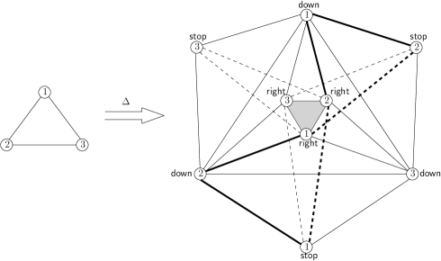
Figure 7: (repeated) The Splitter Task for Three Processes.

0.A.3.3 The Exchanger Task

A second interesting example is the Java exchanger object which is informally defined as follows in the Java documentation:

A synchronization point at which threads can pair and swap elements within pairs. Each thread presents some object on entry to the exchange method, matches with a partner thread, and receives its partner’s object on return.

Clearly the object is informally specified in terms of concurrent executions, very much in the style of the task formalism.

Exchangers have been used in [17] to implement a concurrent stack, and the lack of a sequential specification of exchangers makes the proof in that paper intricate. They have also been used in a number of concurrent implementations, e.g. [24, 36]. More precisely, in [36], Shavit and Touitou present the implementation of pools and stacks with elimination trees, a form of diffracting trees [37] which achieves high efficiency at high contention levels. A simplified version of their algorithm is the following. There are two kinds of opposite requests: enqueue and dequeue for a stack. The structure is constructed from elimination balancers that are connected to one another to form a balanced binary tree. Each leaf of the tree holds a standard concurrent stack implementation (e.g. with locks). Each internal node of the tree holds a prism and an exchanger. The prism has an internal state (0 or 1) and two outputs labelled 0 and 1. It routes a request according to this state: an enqueue request goes on the output labelled as the internal state, a dequeue request goes on the output labelled as the inverse of the internal state. The internal state is flipped after each request. This allows the requests to spread on the tree while ensuring that a dequeue follows the same path as the most recent enqueue. To speed things up and to avoid contention of the internal state, two mechanisms are added. First, two concurrent requests of the same kind are directly routed on both output without changing the internal state. Secondly, an exchanger is used to pair opposite requests: when both an enqueue and a dequeue are present, they are matched, they swap their values and they directly exit the tree without being further propagated (observe that this version of the exchanger is slightly different than the one above as processes exchange opposite requests). The actual implementation uses an array of prisms to avoid the bottleneck of the root and first-levels balancers, however this does not change the overall specification of the algorithm.

Although there is no sequential specification of exchanger in the literature (a proof such as the one for lemma 1 shows that there does not exist such a specification), one can succinctly define it as a task. Intuitively, in order processes exchange values, an exchanger matches pairs of processes, with the possibility that some processes are unmatched (marked as matched with a default value denoted $\bot$). The exchanger task $T_{\mathsf{exc}}=(\mathcal{I}_{\mathsf{exc}},\mathcal{O}_{\mathsf{exc}},\Delta_{\mathsf{exc}})$ is defined as follows.

1. The vertices of the input complex $\mathcal{I}_{\mathsf{exc}}$ are all pairs of the form $(\mbox{\rm id}_{i},\mbox{\rm id}_{i})$, for every ID process $\mbox{\rm id}_{i}$.

2. $\mathcal{I}_{\mathsf{exc}}$ is the complex made of the $n$-dimensional simplex $\{(\mbox{\rm id}_{1},\mbox{\rm id}_{1}),\dots,(\mbox{\rm id}_{n},\mbox{\rm id}_{n})\}$ (and all its faces), with all distinct ID processes $\mbox{\rm id}_{1},\ldots,\mbox{\rm id}_{n}$.

3. The vertices of the output complex $\mathcal{O}_{\mathsf{exc}}$ are all pairs $(\mbox{\rm id}_{i},\mbox{\rm id}_{j})$ and $(\mbox{\rm id}_{i},\bot)$, where $\mbox{\rm id}_{i}$ and $\mbox{\rm id}_{j}$ are distinct process IDs.

4. Given a simplex $\tau=\{(\mbox{\rm id}_{1},y_{1}),\dots,(\mbox{\rm id}_{m},y_{m})\}$ with vertices in $\mathcal{O}_{\mathsf{exc}}$, let $EX(\tau)$ be the exchanger predicate that holds only if

   1. all $\mbox{\rm id}_{i}$’s are distinct,

   2. $\mbox{\rm id}_{i}$ is matched with a different process or not matched at all: $y_{i}\in\{\mbox{\rm id}_{1},\ldots,\widehat{}\mbox{\rm id}_{i},\ldots,\mbox{\rm id}_{m},\bot\}$, where circumflex ($\,\widehat{\,}\,$) denotes omission,

   3. $\mbox{\rm id}_{i}$ is matched with at most one process, namely, it appears in a second entry at most once,

   4. matches are consistent, i.e., if $y_{i}=\mbox{\rm id}_{j}$ then $y_{j}=\mbox{\rm id}_{i}$.

5. $\mathcal{O}_{\mathsf{exc}}$ contains every $n$-dimensional simplex $\tau=\{(\mbox{\rm id}_{1},y_{1}),\dots,(\mbox{\rm id}_{n},y_{n})\}$ (and all its faces) such that $EX(\tau)$ holds.

6. For every $(k-1)$-dimensional input simplex $\sigma$, $\Delta_{\mathsf{exc}}(\sigma)$ contains every $(k-1)$-dimensional output simplex $\tau$ (and all its faces) such that $\mbox{\rm ID}(\tau)=\mbox{\rm ID}(\sigma)$ and $EX(\tau)$ holds.

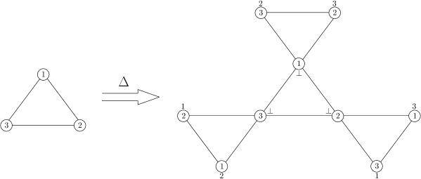
Figure 8: The Exchanger Task for Three Processes.

The exchanger task for three processes with IDs 1, 2 and 3 is depicted in Figure 8. $\Delta$ maps the input vertex $i$ to $(i,\bot)$ and the edge with IDs $i$ and $j$ to the complex with edges $\{(i,\bot),(j,\bot)\}$ and $\{(i,j),(j,i)\}$, and the input triangle is mapped to the whole output complex.

0.A.4 Modeling Tasks as Sequential Objects

Intuitively, tasks and sequential specifications are inherently different paradigms for specifying distributed problems: while a task specifies what a set of processes might output when running concurrently, a sequential specification specifies the behavior of a concurrent object when accessed sequential (and linearizability tells when a concurrent execution “behaves” like a sequential execution of the object).

A natural question is if any task can be modeled as a sequential object with a single operation, namely, the object defines the same set of valid executions. A well-known example for which this is possible is the consensus distributed coordination problem that can be equivalently defined as a task or as a sequential object (see for example [19] where it is defined as an object and [18] where it is defined as a task). Another interesting example is the $\mathsf{Test\&Set}$ atomic operation that is typically specified through a sequential object, however it can also be specified as a task. Figure 9 depicts the $\mathsf{Test\&Set}$ task for three processes (the specification in Figure 6 is not one-shot but it can be easily made one-shot by adding that restriction in the pre-condition). In general, this is not the case, as the following result shows.

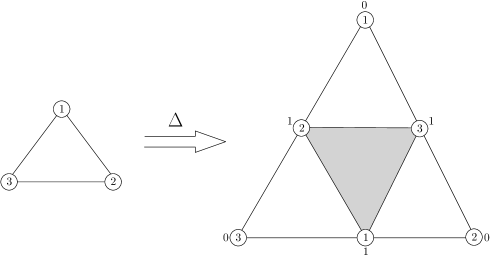
Figure 9: The one-shot $\mathsf{Test\&Set}$ Object for Three Processes Modeled as Task.

Lemma 1 (repeated). Consider the splitter task $T_{\mathsf{spl}}=(\mathcal{I}_{\mathsf{spl}},\mathcal{O}_{\mathsf{spl}},\Delta_{\mathsf{spl}})$. There is no sequential object $X_{\mathsf{spl}}$ with a single operation satisfying:

$$VE(T_{\mathsf{spl}})=VE(X_{\mathsf{spl}}).$$

Proof

Suppose by contradiction that there is such an object $X_{\mathsf{spl}}$ and consider the following fully concurrent execution for three processes:

$$\begin{array}[]{ll}E=&inv(p_{1},p_{1});inv(p_{2},p_{2});inv(p_{3},p_{3});resp(p_{1}):\mathsf{down};resp(p_{2}):\mathsf{down};\\ &resp(p_{3}):\mathsf{right}.\end{array}$$

For a prefix $E^{\prime}$ of $E$, one can verify that $\tau_{E^{\prime}}\in\Delta_{\mathsf{spl}}(\sigma_{E^{\prime}})$; for example, $\sigma_{E}=\{(p_{1},p_{1}),(p_{2},p_{2}),(p_{3},p_{3})\}$, $\tau_{E}=\{(p_{1},\mathsf{down}),(p_{2},\mathsf{down}),(p_{3},\mathsf{right})\}$ and $\tau_{E}\in\Delta_{\mathsf{spl}}(\sigma_{E})$. Then, $E$ satisfies $T_{\mathsf{spl}}$, from which follows that $E\in VE(T_{\mathsf{spl}})$.

Now, our assumption implies that $E\in VE(X_{\mathsf{spl}})$, thus $E$ is linearizable with respect to $X_{\mathsf{spl}}$. Without loss of generality suppose that there is a linearization $S$ of $E$ in which $inv(p_{1},p_{1});resp(p_{1}):\mathsf{down}$ is the first linearized operation. Thus, $S$ is a sequential execution of $X_{\mathsf{spl}}$, namely, $S\in SSpec(X_{\mathsf{spl}})$. Since $SSpec(X_{\mathsf{spl}})$ is prefix-closed and $F=inv(p_{1},p_{1});resp(p_{1}):\mathsf{down}$ is a prefix of $S$, we have that $F\in SSpec(X_{\mathsf{spl}})$. This is a contradiction because $F$ is indeed an execution which is linearizable with respect to $X_{\mathsf{spl}}$ ($F$ is a linearization of itself), hence $F\in VE(X_{\mathsf{spl}})$, but F does not satisfy $T_{\mathsf{spl}}$ (clearly $\tau_{F}\notin\Delta_{\mathsf{spl}}(\sigma_{F})$), and thus $F\notin VE(T_{\mathsf{spl}})$, which is a contradiction.

In a very similar way one can prove that the exchanger task defined above and the following known tasks cannot be specified as sequential objects with a single operation:

1. Adaptive renaming [4]. Processes start with distinct inputs names taken from the space $[1,\ldots,N]$ and decide distinct outputs names from the space $[1,\ldots,M]$, with $N>>M$. It is required that if $k\leq n$ processes run concurrently, the output names belong to $[1,\ldots,f(k)]$, for some function $f:{1,\ldots,n}\rightarrow\{1,\ldots,N\}$, i.e., the output space is on function on the number of participating processes.

2. Set agreement [10]. It is a generalization of the well-known consensus where processes propose values and have to agree on at most $k$ proposals.

3. Immediate snapshot [5]. It is a task which plays an important role in distributed computability [18]. A process can write a value to the shared memory using this operation, and gets back a snapshot of the shared memory, such that the snapshot occurs immediately after the write.

4. Adopt-commit [6, 13] is a concurrent object which proved to be is useful to simulate round-based protocols for set-agreement and consensus. Given an input $u$ to the object, the result is an output of the form $(commit,v)$ or $(adopt,v)$, where $commit/adopt$ is a decision that indicates whether the process should decide value $v$ immediately or adopt it as its preferred value in later rounds of the protocol.

5. Conflict detection [3] is a task that has been shown to be equivalent to the adopt-commit. Roughly, if at least two different values are proposed concurrently at least one process outputs true.

To circumvent the impossibility result in the previous lemma, we model any given task $T$ through a sequential object $S$ with two operations, $\mathsf{set}$ and $\mathsf{get}$, that each process access in a specific way: it first invokes set with its input to the task $T$ (receiving no output) and later invokes $\mathsf{get}$ in order to get an output value from $T$. Intuitively, decoupling the single operation of $T$ into two (atomic) operations allows us to model concurrent behaviors that a single (atomic) operation cannot specify. In what follows, let $SSpec(S)$ be the set with all sequential executions of $S$ in which each process invokes at most two operations, first $\mathsf{set}$ and then $\mathsf{get}$, in that order.

Theorem 3.1 (repeated). For every task $T=(\mathcal{I},\mathcal{O},\Delta)$ there is a sequential object $S$ with two operations, $\mathsf{set}$$(\mbox{\rm id}_{i},x_{i})$ and $\mathsf{get}$$(\mbox{\rm id}_{i}):y_{i}$, such that there is a bijection $\alpha$ between $VE(T)$ and $SSpec(S)$ satisfying that

1. each invocation or response of process $\mbox{\rm id}_{i}$ is mapped to an operation of process $\mbox{\rm id}_{i}$,

2. each invocation $inv$ (response $resp$) with input (output) $x$ is mapped to a completed $\mathsf{set}$ ($\mathsf{get}$) operation with input (output) $x$.

Proof

We define $S$ as follows. The sets of invocation and responses, $Inv$ and $Res$, of $S$ contain $inv(\mathsf{set},\mbox{\rm id}_{i},x_{i})$ and $res(\mathsf{set},\mbox{\rm id}_{i},x_{i}):{\sf void}$, respectively, for each input vertex $(\mbox{\rm id}_{i},x_{i})\in\mathcal{I}$. Similarly, for each output vertex $(\mbox{\rm id}_{i},y_{i})\in\mathcal{O}$, $Inv$ and $Res$ contain $inv(\mathsf{get},\mbox{\rm id}_{i})$ and $res(\mathsf{get},\mbox{\rm id}_{i}):y_{i}$.

For every execution $E\in VE(T)$, $S$ has a state $s_{E}$ and the initial state of $S$ is $s_{\xi}$, where $\xi$ denotes the empty string. We define the transition function $\delta$ of $S$ inductively as:

1. For every execution $E\in VE(T)$ consisting of only one invocation $inv(\mbox{\rm id}_{i},x_{i})$ (i.e. $E=inv(\mbox{\rm id}_{i},x_{i})$), we define

   $$\delta(s_{\xi},inv(\mathsf{set},\mbox{\rm id}_{i},x_{i}))=\{(s_{E},res(\mathsf{set},\mbox{\rm id}_{i},x_{i}):{\sf void})\}.$$

2. For every execution $E\in VE(T)$ with the form $E=E^{\prime}\cdot e$, for some non-empty $E^{\prime}$ prefix, $\delta$ is defined as:

   1. If $e=inv(\mbox{\rm id}_{i},x_{i})$, then

      $$\delta(s_{E^{\prime}},inv(\mathsf{set},\mbox{\rm id}_{i},x_{i}))=\{(s_{E^{\prime}\cdot e},res(\mathsf{set},\mbox{\rm id}_{i},x_{i}):{\sf void})\}.$$

   2. If $e=res(\mbox{\rm id}_{i}):y_{i}$, then

      $$\delta(s_{E^{\prime}},inv(\mathsf{get},\mbox{\rm id}_{i}))=\{(s_{E^{\prime}\cdot e},res(\mathsf{get},\mbox{\rm id}_{i}):y_{i})\}.$$

Observe that $S$ is a deterministic automaton whose sequential executions are precisely the executions in $VE(T)$ (one can think that $S$ is an automaton that recognizes the language $VE(T)$). Moreover, each invocation $(\mbox{\rm id}_{i},x_{i})$ in an execution in $VE(T)$ induces a transition in $S$ with an invocation to $\mathsf{set}$$(\mbox{\rm id}_{i},x_{i})$ and, similarly, each response $(\mbox{\rm id}_{i},y_{i})$ in an execution in $VE(T)$ induces a transition in $S$ with an invocation to $\mathsf{get}$$(\mbox{\rm id}_{i})$ whose response value is $y_{i}$. Thus, the desired bijection $\alpha$ in $VE(T)\rightarrow SSeq(S)$ is precisely obtained from the definition of $S$.

State: a pair $(\sigma,\tau)$ of input/output simplexes, initialized to $(\emptyset,\emptyset)$
Function $\mathsf{set}$($\mbox{\rm id}_{i},x_{i}$)
	Pre-condition:
		$\mbox{\rm id}_{i}\in\mbox{\rm ID}\wedge\mbox{\rm id}_{i}\notin\mbox{\rm ID}(\sigma)$
	Post-condition:
		$\sigma^{\prime}\leftarrow\sigma\cup\{(\mbox{\rm id}_{i},x_{i})\}$
	Output:
		$\sf void$
endFunction
Function $\mathsf{get}$($\mbox{\rm id}_{i}$)
	Pre-condition:
		$\mbox{\rm id}_{i}\in\mbox{\rm ID}\wedge\mbox{\rm id}_{i}\notin\mbox{\rm ID}(\tau)$
	Post-condition:
		Let $y_{i}$ be any output value such that $\tau\cup\{(\mbox{\rm id}_{i},y_{i})\}\in\Delta(\sigma)$
		$\tau^{\prime}\leftarrow\tau\cup\{(\mbox{\rm id}_{i},y_{i})\}$
	Output:
		$y_{i}$
endFunction

Figure 10: (repeated) A Generic Sequential Specification of a Task $T=(\mathcal{I},\mathcal{O},\Delta)$.

An implication of Theorem 3.1 is that if one is analyzing an algorithm that uses a building-block (subroutine, algorithm, etc.) $B$ that solves a task $T$, one can safely replace $B$ with the sequential object $S$ related to $T$ described in the theorem (each invocation to the operation $B$ is replaced with an (atomic) invocation to $\mathsf{set}$ and then an (atomic) invocation to $\mathsf{get}$), and then analyze the algorithm considering the atomic operations of $S$. The advantage of this transformation is that (1) if all operations in an algorithm are atomic, we can think that each process takes a step at a time in an execution, hence obtaining a transition system with atomic events, (2) at all times we have a concrete state of $S$ in an execution (which is not clear in a task specification) and (3) given a state of $S$, an output for a $\mathsf{get}$ operation can be easily computed using the sequential object $S$ (something that is typically complicated for $B$ as it might be accessed concurrently). In light of this, the construction used (for simplicity) in the proof of Theorem 3.1 might be too coarse to be helpful for analyzing an algorithm. Thus, we would like to have a construction producing an equivalent sequential automaton modeling the task in a simpler way.

Consider the sequential object in Figure 5 obtained from any given task $T=(\mathcal{I},\mathcal{O},\Delta)$, which is described in a classic pre/post-condition form. Intuitively, the meaning of a state $(\sigma,\tau)$ is the following: $\sigma$ contains the processes that have invoked the task so far (this represents the participating set of the current execution) while $\tau$ contains the outputs that have been produced so far. The main invariant of the specification is that $\tau\in\Delta(\sigma)$. It directly follows from the properties of the task: when a process invokes $\mathsf{set}$$(\mbox{\rm id}_{i},x_{i})$, we have that $\tau\in\Delta(\sigma\cup\{(\mbox{\rm id}_{i},x_{i})\})$ because $\Delta(\sigma)\subset\Delta(\sigma\cup\{(\mbox{\rm id}_{i},x_{i})\})$, and when a process invokes $\mathsf{get}$$(\mbox{\rm id}_{i})$, it holds that $\tau\cup\{(\mbox{\rm id}_{i},y_{i})\}\in\Delta(\sigma)$ because $\Delta(\sigma)$ is pure of dimension $\mbox{\sl dim}(\sigma)$ and thus there must exist a simplex in $\Delta(\sigma)$ (properly) containing $\tau$ and with an output for $\mbox{\rm id}_{i}$. One can formally prove that this sequential object and the one in the proof Theorem 3.1 define the same set of sequential executions.

The formal definition of the sequential object in Figure 5 is the following.

1. For every $\sigma\in\mathcal{I}$, and for every $\tau\in\mathcal{O}$, $q_{(\sigma,\tau)}$ is a state in $Q$. The initial state is $q_{(\emptyset,\emptyset)}$.

2. For every input vertex $(\mbox{\rm id}_{i},x_{i})\in\mathcal{I}$, $inv(\mathsf{set},\mbox{\rm id}_{i},x_{i})\in Inv$ and $res(\mathsf{set},\mbox{\rm id}_{i},x_{i}):{\sf void}\in Res$.

3. For each output vertex $(\mbox{\rm id}_{i},y_{i})\in\mathcal{O}$, $inv(\mathsf{get},\mbox{\rm id}_{i})\in Inv$ and $res(\mathsf{get},\mbox{\rm id}_{i}):y_{i}\in Res$.

4. For every state $q_{(\sigma,\tau)}$,

   1. for every $(\mbox{\rm id}_{i},x_{i})$ such that $\mbox{\rm id}_{i}\notin\mbox{\rm ID}(\sigma)$ and $\sigma\cup\{(id_{i},x_{i})\}\in\mathcal{I}$,

      $$\delta(q_{(\sigma,\tau)},inv(\mathsf{set},\mbox{\rm id}_{i},x_{i}))=\{(q_{(\sigma\cup\{(id_{i},x_{i})\},\tau)},res(\mathsf{set},\mbox{\rm id}_{i},x_{i}):{\sf void})\},$$

   2. for every $(\mbox{\rm id}_{i},y_{i})$ such that $\mbox{\rm id}_{i}\in\mbox{\rm ID}(\sigma)$, $\mbox{\rm id}_{i}\notin\mbox{\rm ID}(\tau)$ and $\tau\cup\{(id_{i},y_{i})\}\in\Delta(\sigma)$,

      $$(q_{(\sigma,\tau\cup\{(id_{i},y_{i})\})},res(\mathsf{get},\mbox{\rm id}_{i}):y_{i})\in\delta(q_{(\sigma,\tau)},inv(\mathsf{get},\mbox{\rm id}_{i})).$$

Finally, one can obtain simpler and equivalent specifications for specific tasks, like we did for the splitter in Section 2. Figure 11 presents such a specification where $\sigma$ is represented with the set $Participants$, $\tau$ with the sets $Stop,Down$ and $Right$ and the splitter predicate in the task is literally expressed in the get operation. An ad hoc sequential specification of the exchanger is depicted in Figure 12 (a slight variation gives the exchanger used in [36]).

State: Sets $Participants,Stop,Down,Right$, all initialized to $\emptyset$
Function $\mathsf{set}$(id)
	Pre-condition:
		$\mbox{\rm id}\notin Participants$
	Post-condition:
		$Participants^{\prime}\leftarrow Participants\cup\{\mbox{\rm id}\}$
	Output:
		$\sf void$
endFunction
Function $\mathsf{get}$(id)
	Pre-condition:
		$\mbox{\rm id}\in Participants\wedge\mbox{\rm id}\notin Stop,Down,Right$
	Post-condition:
		$D\leftarrow\emptyset$
		if $|Stop|=0$ then $D\leftarrow D\cup\{\mathsf{stop}\}$
		if $|Down|<|Participants|-1$ then $D\leftarrow D\cup\{\mathsf{down}\}$
		if $|Right|<|Participants|-1$ then $D\leftarrow D\cup\{\mathsf{right}\}$
		Let $dec$ be any value in $D$
		if $dec=\mathsf{stop}$ then $Stop\leftarrow Stop\cup\{\mbox{\rm id}\}$
		if $dec=\mathsf{down}$ then $Down\leftarrow Down\cup\{\mbox{\rm id}\}$
		if $dec=\mathsf{right}$ then $Right\leftarrow Right\cup\{\mbox{\rm id}\}$
	Output:
		$dec$
endFunction

Figure 11: (repeated) An ad hoc Specification of the Splitter Task.

Correctness and Completeness.

In the light of the ad hoc sequential specifications in Figures 11 and 12, consider the following question: how can we know if a given sequential specification $X$ with $\mathsf{get}$ and $\mathsf{set}$ operations corresponds to a task $T$, namely, it actually models $T$? That is to say, we consider the direction opposite to Theorem 3.1, from sequential objects to tasks. One way to obtain such a result is to show that there is an isomorphism between $X$ and the sequential automaton, say $S_{T}$, obtained from the generic construction of Figure 10, instantiated with $T$. A second equivalent approach is to verify that $X$ is correct, i.e., it satisfies the input/output relation of $T$, and complete, namely, it specifies all possible executions in $VE(T)$. Satisfying these two properties implies that $X$ and $S_{T}$ are isomorphic.

Formally, $X$ is correct w.r.t.$T$ if, for each of its executions $E\in SSpec(X)$, $\tau_{E}\in\Delta(\sigma_{E})$, where $\sigma_{E}$ is the simplex containing an invocation to $T$ for each (complete) $\mathsf{set}$ operation of $X$ in $E$, with same process and input value, and, similarly, $\tau_{E}$ is the simplex containing a response from $T$ for each (complete) $\mathsf{get}$ operation of $X$ in $E$, with same process output value.

We say that $X$ is complete w.r.t.$T$ if for each execution of $E\in VE(T)$, $S_{E}\in SSpec(X)$, where $S_{E}$ is the sequential execution obtained from $E$ by replacing each invocation to $T$ in $E$ with a complete $\mathsf{set}$ operation of $X$, with same process and input value, and each response from $T$ in $E$ with a complete $\mathsf{get}$ operation of $X$, with same process and output value.

State: Sets $Participants,Matching$, both initialized to $\emptyset$
Function $\mathsf{set}$(id)
	Pre-condition: $\mbox{\rm id}\notin Participants$
	Post-condition: $Participants^{\prime}\leftarrow Participants\cup\{\mbox{\rm id}\}$
	Output: $\sf void$
endFunction
Function $\mathsf{get}$(id)
	Pre-condition: $\mbox{\rm id}\in Participants\wedge\{\mbox{\rm id},\cdot\}\notin Matching$
	Post-condition:
		$Matched\leftarrow\{\mbox{\rm id}^{\ast}|\{\mbox{\rm id}^{\ast},\cdot\}\in Matching\}$
		$Free\leftarrow Participants\setminus Matched$
		if $\mbox{\rm id}\in Matched$ then
			Let $\mbox{\rm id}^{\ast}$ be the value in Matched such that $\{\mbox{\rm id},\mbox{\rm id}^{\ast}\}\in Matched$
		else
			Let $\mbox{\rm id}^{\ast}$ be any value in $Free\cup\{\bot\}$
			$Matching^{\prime}\leftarrow Matching\cup\{\{\mbox{\rm id},\mbox{\rm id}^{\ast}\}\}$
	Output: $\mbox{\rm id}^{\ast}$
endFunction

Figure 12: An ad hoc Specification of the Exchanger.

On Adaptiveness.

An interesting property of the splitter and ${\sf Test\&Set}$ sequential objects in Figures 6 and 3 is that they do not take into account the number of processes in the system, namely, the specification is the same for any number of processes. This property is known as adaptiveness and can be formalized as follows.

Consider an infinite set of processes $\mbox{\rm ID}=\{p_{1},p_{2},\ldots\}$. Consider a distributed problem that is specified through an infinite family of sequential objects: for every finite set $S\subset\mbox{\rm ID}$, let $X_{S}$ be a sequential object for processes in $S$. The family of objects is adaptive if for every two sets $S\subset S^{\prime}$, $SSpec(X_{S})=SSpec(X_{S^{\prime}},S)$, where $SSpec(X_{S^{\prime}},S)$ is the subset of $SSpec(X_{S^{\prime}})$ with operations of processes in $S$.

The notion of adaptiveness for tasks is defined similarly. Consider a distributed problem that is specified through an infinite family of tasks: for every finite set $S\subset\mbox{\rm ID}$, let $T_{S}=(\mathcal{I}_{S},\mathcal{O}_{S},\Delta_{S})$ be a sequential object for processes in $S$. The family of tasks is adaptive if for every two sets $S\subset S^{\prime}$, $\mathcal{I}_{S}\subset\mathcal{I}_{S^{\prime}}$ and for every $\sigma\in\mathcal{I}_{S}$, $\Delta_{S}(\sigma)=\Delta_{S^{\prime}}(\sigma)$.

References

- [1] Dan Alistarh. The renaming problem: Recent developments and open questions. Bulletin of the EATCS, 117, 2015.
- [2] Manamiary Bruno Andriamiarina, Dominique Méry, and Neeraj Kumar Singh. Revisiting snapshot algorithms by refinement-based techniques. Computer Science and Information Systems, 11(1):251–270, 2014.
- [3] James Aspnes and Faith Ellen. Tight bounds for adopt-commit objects. Theory Comput. Syst., 55(3):451–474, 2014.
- [4] Attiya H., Bar-Noy A., Dolev D., Peleg D. and Reischuk R. Renaming in an asynchronous environment. Journal of the ACM, 37(3):524–548, 1990.
- [5] Elizabeth Borowsky and Eli Gafni. Generalized FLP impossibility result for t-resilient asynchronous computations. In STOC ’93: Proceedings of the ACM Symposium on Theory of computing, pages 91–100, New York, NY, USA, 1993. ACM.
- [6] Elizabeth Borowsky, Eli Gafni, Nancy A. Lynch, and Sergio Rajsbaum. The BG distributed simulation algorithm. Distributed Computing, 14(3):127–146, 2001.
- [7] Armando Castañeda, Aurélie Hurault, Philippe Quéinnec, and Matthieu Roy. Tasks in modular proofs of concurrent algorithms. CoRR, arXiv:1909.05537 [cs.DC], 2019.
- [8] Armando Castañeda, Sergio Rajsbaum, and Michel Raynal. The renaming problem in shared memory systems: An introduction. Computer Science Review, 5(3):229–251, 2011.
- [9] Armando Castañeda, Sergio Rajsbaum, and Michel Raynal. Unifying concurrent objects and distributed tasks: Interval-linearizability. J. ACM, 65(6):45:1–45:42, 2018.
- [10] Soma Chaudhuri. More choices allow more faults: Set consensus problems in totally asynchronous systems. Inf. Comput., 105(1):132–158, July 1993.
- [11] Sylvain Conchon, Amit Goel, Sava Krstic, Alain Mebsout, and Fatiha Zaïdi. Cubicle: A parallel SMT-based model checker for parameterized systems. In Computer Aided Verification - 24th International Conference, CAV 2012, volume 7358 of LNCS, pages 718–724, 2012.
- [12] Cezara Dragoi, Ashutosh Gupta, and Thomas A. Henzinger. Automatic linearizability proofs of concurrent objects with cooperating updates. In Conference on Computer Aided Verification - 25th International Conference, CAV 2013, volume 8044 of Lecture Notes in Computer Science, pages 174–190. Springer, 2013.
- [13] Eli Gafni. Round-by-round fault detectors: Unifying synchrony and asynchrony (extended abstract). In Proceedings of the Seventeenth Annual ACM Symposium on Principles of Distributed Computing, PODC ’98, pages 143–152, 1998.
- [14] Silvio Ghilardi and Silvio Ranise. MCMT: A model checker modulo theories. In 5th International Joint Conference on Automated Reasoning IJCAR, volume 6173 of Lecture Notes in Computer Science, pages 22–29. Springer, 2010.
- [15] Éric Goubault, Jérémy Ledent, and Sergio Rajsbaum. A simplicial complex model for dynamic epistemic logic to study distributed task computability. In Ninth International Symposium on Games, Automata, Logics, and Formal Verification, GandALF 2018, pages 73–87, 2018.
- [16] Nir Hemed, Noam Rinetzky, and Viktor Vafeiadis. Modular verification of concurrency-aware linearizability. In Distributed Computing - 29th International Symposium, DISC 2015, pages 371–387, 2015.
- [17] Danny Hendler, Nir Shavit, and Lena Yerushalmi. A scalable lock-free stack algorithm. J. Parallel Distrib. Comput., 70(1):1–12, 2010.
- [18] Maurice Herlihy, Dmitry N. Kozlov, and Sergio Rajsbaum. Distributed Computing Through Combinatorial Topology. Morgan Kaufmann, 2013.
- [19] Maurice Herlihy and Nir Shavit. The art of multiprocessor programming. Morgan Kaufmann, 2008.
- [20] Maurice Herlihy and Jeannette M. Wing. Linearizability: A correctness condition for concurrent objects. ACM Trans. Program. Lang. Syst., 12(3):463–492, 1990.
- [21] Gerard J. Holzmann. The SPIN Model Checker - primer and reference manual. Addison-Wesley, 2004.
- [22] Aurélie Hurault and Philippe Quéinnec. Proving a non-blocking algorithm for process renaming with TLA+. In 13th International Conference on Tests and Proofs, TAP 2019, October 2019.
- [23] IEC. IEC-61508: Functional safety. https://www.iec.ch/functionalsafety/.
- [24] William N. Scherer III, Doug Lea, and Michael L. Scott. Scalable synchronous queues. Commun. ACM, 52(5):100–111, 2009.
- [25] William N. Scherer III and Michael L. Scott. Nonblocking concurrent data structures with condition synchronization. In Distributed Computing, 18th International Conference, DISC 2004, pages 174–187, 2004.
- [26] Annu John, Igor Konnov, Ulrich Schmid, Helmut Veith, and Josef Widder. Parameterized model checking of fault-tolerant distributed algorithms by abstraction. In Formal Methods in Computer-Aided Design, FMCAD 2013, pages 201–209. IEEE, October 2013.
- [27] Leslie Lamport. Specifying Systems. Addison Wesley, 2002.
- [28] Leslie Lamport. Byzantizing paxos by refinement. In 25th International Symposium on Distributed Computing, DISC 2011, volume 6950 of Lecture Notes in Computer Science, pages 211–224. Springer, 2011.
- [29] Tianxiang Lu. Formal Verification of the Pastry Protocol. PhD thesis, Université de Lorraine – Universität des Saarlandes, July 2013.
- [30] Tianxiang Lu, Stephan Merz, and Christoph Weidenbach. Towards verification of the Pastry protocol using TLA+. In International Conference on Formal Techniques for Distributed Systems FORTE, volume 6722 of Lecture Notes in Computer Science, pages 244–258. Springer, 2011.
- [31] Mark Moir and James H. Anderson. Wait-free algorithms for fast, long-lived renaming. Science of Computer Programming, 25(1):1–39, 1995.
- [32] Mark Moir, Daniel Nussbaum, Ori Shalev, and Nir Shavit. Using elimination to implement scalable and lock-free FIFO queues. In 17th ACM Symposium on Parallelism in Algorithms and Architectures, SPAA 2005, pages 253–262. ACM, 2005.
- [33] Gil Neiger. Set-linearizability. In Proceedings of the Thirteenth Annual ACM Symposium on Principles of Distributed Computing, Los Angeles, California, USA, August 14-17, 1994, page 396, 1994.
- [34] Peter W. O’Hearn, Noam Rinetzky, Martin T. Vechev, Eran Yahav, and Greta Yorsh. Verifying linearizability with hindsight. In 29th Annual ACM Symposium on Principles of Distributed Computing, PODC 2010, pages 85–94. ACM, 2010.
- [35] Michel Raynal. Concurrent Programming - Algorithms, Principles, and Foundations. Springer, 2013.
- [36] Nir Shavit and Dan Touitou. Elimination trees and the construction of pools and stacks. Theory Comput. Syst., 30(6):645–670, 1997.
- [37] Nir Shavit and Asaph Zemach. Diffracting trees. ACM Transactions on Computer Systems, 14(4):385–428, 1996.
- [38] Bogdan Tofan, Gerhard Schellhorn, and Wolfgang Reif. A compositional proof method for linearizability applied to a wait-free multiset. In Integrated Formal Methods - 11th International Conference, IFM 2014, volume 8739 of Lecture Notes in Computer Science, pages 357–372. Springer, 2014.
- [39] Pamela Zave. Using lightweight modeling to understand Chord. SIGCOMM Computer Communication Review, 42(2):49–57, April 2012.