Differential Approximation and Sprinting for Multi-Priority Big Data Engines

Abstract.

Today’s big data clusters based on the MapReduce paradigm are capable of executing analysis jobs with multiple priorities, providing differential latency guarantees. Traces from production systems show that the latency advantage of high-priority jobs comes at the cost of severe latency degradation of low-priority jobs as well as daunting resource waste caused by repetitive eviction and re-execution of low-priority jobs. We advocate a new resource management design that exploits the idea of differential approximation and sprinting. The unique combination of approximation and sprinting avoids the eviction of low-priority jobs and its consequent latency degradation and resource waste. To this end, we designed, implemented and evaluated DiAS, an extension of the Spark processing engine to support deflate jobs by dropping tasks and to sprint jobs. Our experiments on scenarios with two and three priority classes indicate that DiAS achieves up to 90% and 60% latency reduction for low- and high-priority jobs, respectively. DiAS not only eliminates resource waste but also (surprisingly) lowers energy consumption up to 30% at only a marginal accuracy loss for low-priority jobs.

1. Introduction

Big data production systems, e.g., Google (Wilkes, 2011) and Facebook (Chen et al., 2012), implement priority scheduling to process job streams with different characteristics and latency requirements. Analysis jobs, e.g., hive queries (Ganapathi et al., 2010) and text mining, of different priorities arrive in streams and are executed as parallel jobs with varying numbers of map and reduce tasks. Trace studies (Çavdar et al., 2014) show that high-priority jobs are promptly served with little queueing time, while low-priority jobs suffer from repetitive evictions causing significant resource waste. This can be attributed to the practice of preemptive priority scheduling (Schwarzkopf et al., 2013), where high-priority jobs are given the ability to preempt lower-priority jobs in execution. The average latency slowdown of low-priority jobs (Rosà et al., 2015a), i.e., the end-to-end response time divided by the execution time excluding eviction, can be 3$\times$ higher than for high-priority jobs. All in all, priority-enabled big data systems preserve the performance advantage of high-priority jobs at the cost of resource efficiency and performance of low-priority jobs.

It is extremely challenging to optimize the performance of big data engines with priority scheduling as performance conflicts arise across disparate job priorities as well as across performance targets, i.e., latency vs. resource efficiency. Meeting the latency targets in priority systems is a long standing challenge from both system (Schwarzkopf et al., 2013; Cho et al., 2013) and modelling (Harchol-Balter et al., 2005; Horváth, 2015) perspectives due to the complex dynamics and performance requirements across diverse priority classes. This is partly because the processing order of low-priority jobs highly depends on the high-priority jobs, especially when low-priority jobs are evicted during periods of resource shortage. In additional to the inter-job dependency, big data jobs themselves have complex execution dynamics across their parallel tasks and synchronization stages.

Existing systems address the latency issue of big data engines mainly from the perspective of single job type, i.e., one single priority. On the one hand, approximation-enabled processing engines, e.g., BlinkDB (Agarwal et al., 2013) and ApproxHadoop (Goiri et al., 2015), reduce the execution times by processing a fraction of input data. The performance advantage comes at the cost of accuracy losses. On the other hand, hardware features are increasingly being exploited to accelerate the executions of jobs. For example, Pupil (Zhang and Hoffmann, 2016) and Sprinting Game (Fan et al., 2016) temporarily sprint the CPU frequency during the slow execution phases of jobs. However, these engines do not readily apply to multi-priority scenarios, answering the performance and resource tradeoff among different priorities.

We advocate to differentially approximate and sprint CPU frequency for jobs of different priorities, termed differential approximation and sprinting (DiAS), to replace preemptive eviction in priority scheduling. DiAS improves the latency for all priorities and eliminates resource waste from re-executing the evicted low-priority jobs. To achieve this, DiAS reduces a fraction of data load for low-priority jobs and temporarily increase the CPU frequency for high-priority jobs.

The differential approximation adopts a controllable approximation level that discriminates among priority classes by dropping different fractions of data. It gives better latencies for low-priority jobs at the cost of their accuracy loss and minor latency increase for high-priority jobs, depending on the levels of input data dropping. The differential sprinting then adjusts the frequency levels such that the high-priority jobs can be accelerated after temporarily waiting behind the low-priority approximate jobs.

We design, implement and evaluate DiAS on top of Spark (Zaharia et al., 2016). The DiAS extension module is composed of $N$ priority buffers, and one deflator that assigns approximation and sprinting levels for each priority. To determine the dropping and frequency levels, we derive a set of stochastic models that can predict average response times of DiAS jobs. The models, based on matrix-analytic methods and parameterized via simple linear regressions, can effectively guide the choice of approximation levels for each priority.

We evaluate DiAS using benchmarks that process the contents of the stackexchange (sta, 2019) network of question-and-answer websites as well as the Google web graph (goo, 2019), with two and three job priority levels. To demonstrate the robustness of DiAS, we consider various workload profiles, i.e., priority ratios, job sizes, and system loads. Evaluation results show that DiAS achieves remarkable reductions not only on the mean and tail latency of low-priority jobs, but also on the tail latency of high-priority jobs. With DiAS we achieve up to 90% and 60% reduction in the mean/tail latency for low-priority and high priority jobs, respectively, a preemptive priority system without approximation and sprinting. Moreover, the promising performance gain of DiAS comes with a noticeable energy reduction energy, i.e., up to 30% , even after spending extra power to sprint the high priority jobs.

Our contributions are multi-fold. First, we put forward a first of its kind design for differential approximation and sprinting that preserves the latency advantage of high-priority jobs and reverts the latency disadvantage of low-priority jobs for both mean and tail latencies. Second, we derive bottom-up stochastic models that capture the dynamics of big data jobs (at both the task and the stage levels) that implement different approximation and sprinting levels. Third, we implemented DiAS on top of Spark, the state-of-the-art big data processing engine, by building a model-based job deflator and augmenting Spark with the approximation capability of dropping tasks. Last, DiAS agilely combines multiple knobs (task dropping, sprinting, and scheduling) to achieve significant latency and energy reduction from the state of the art.

2. Motivation and Background

Here, we first use traces collected from production systems to motivate the performance pitfall of preemptive priority scheduling, i.e., resource waste from evicting low priority jobs. We then discuss the background of priority scheduling, big data processing engines to highlight their complexity, and computational sprinting.

2.1. Resource Waste in Production Systems

A number of field studies (Rosà et al., 2015a; Rosà et al., 2015b; Wilkes, 2011; Schwarzkopf et al., 2013) from publicly available big data cluster traces show that priority scheduling is widely adopted in production big data systems. Workloads are defined in the unit of jobs that are in turn composed of multiple tasks. Jobs are divided into multiple classes, each of which is assigned with a priority level. For example, Google clusters employ 12 priority levels (Schwarzkopf et al., 2013). Performance of high-priority jobs is typically enforced at the cost of low-priority jobs. Earlier studies (Rosà et al., 2015b) show that jobs with the lowest priority (priority 0) are repetitively evicted by the scheduler, due to the arrival of high priority workloads. The unfortunate consequences of eviction in production systems are two-fold: (i) high amount of resources, i.e., 25% machine and 30% CPU time, are spent/wasted on subsequent evictions; (ii) significant latency degradation for low priority jobs, e.g., the slowdown of priority-0 jobs compared to the case of no eviction is 3 times higher than that of priority-6 jobs. Differential approximation eliminates this resource waste as low-priority jobs are never evicted. Instead, low priority jobs are processed approximately to provide short response times and to allow high-priority jobs to quickly gain access to processing slots.

2.2. Priority Scheduling

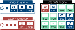
It is of paramount importance to optimize the priority scheduler, especially when encountering big data workloads with strong inter- and intra-priority dynamicity (Chen et al., 2012; Schwarzkopf et al., 2013). Priority schedulers typically separate jobs by their priority levels and keep them in separate queues. Then, they determine when and which job to process next Figure 1 depicts the schematics of a big data cluster with multiple slots serving high- and low-priority jobs in two queues. Jobs arrive with a number of parallel tasks, following MapReduce (Dean and Ghemawat, 2008) programming paradigm and having time-varying arrival rates. Jobs with the same priority class stay in the same queue and are typically served in a first-come-first-served (FCFS) manner. Across priorities, jobs with a higher priority have precedence over any job with a lower priority. Upon arrival of a high priority job, the scheduler ensures that it is served quickly by either evicting any lower priority jobs currently being processed, or by letting the current lower priority jobs to finish and immediately start the incoming job. The former is called preemptive, whereas the latter is termed non-preemptive priority scheduling. As observed in (Rosà et al., 2015b), the Google production systems employ preemptive priority scheduling, causing significant resource waste due to evictions. After being evicted, low-priority jobs return to the head of the queue and wait for new scheduling opportunities, i.e., until no high-priority job is queued or processed. These evictions are completely avoided by differential approximation as it employs non-preemptive scheduling, with the consequent resource savings.

2.3. Computational Sprinting

Figure 1. Schematics of priority scheduling for big data jobs.

Computational sprinting allows for bursts of peak performance under a sprinting budget. The sprinting budget can stem from thermal (Rotem et al., 2012), power (Fan et al., 2016) or provisioning (AWS, 2019) constraints. Several sprinting mechanisms exist, from modifying the CPU performance via dynamic voltage and frequency scaling (DVFS) (Rotem et al., 2012) to tuning the job parallelism (Haque et al., 2015). The common aim is to temporarily accelerate the execution of a job. Each sprinting mechanism is controlled via a corresponding sprinting policy which determines what and when to sprint. Time-based policies levering timeouts to control the sprinting are rather common (Hsu et al., 2015; Morris et al., 2018).

2.4. Processing Engines and MapReduce Jobs

MapReduce is a parallel programming paradigm to process data at scale. Spark (Spa, 2019) is a popular open source implementation of this paradigm with additional support for fast iterative computations and fault tolerance mechanisms. A typical MapReduce job processes input data and returns analysis results via parallel tasks executed in multiple map and reduce stages. The input data are organized as blocks stored in a file system, such as the Hadoop File System (HDFS) (Shvachko et al., 2010), which splits data across the servers in the cluster. During a map stage, map tasks are spawned to process one input block each. Intermediate results are stored as key-value pairs. Afterwards, reduce tasks access and aggregate the intermediate key-value pairs for the final result. A job can comprise multiple such map and reduce tasks/stages. Specific policies supported by cluster job scheduler exist to allow one or multiple concurrent jobs in the engine, respectively for FCFS and weighted fair sharing.

DiAS provides a turnkey solution compatible with the plethora of existing scheduling frameworks and job schedulers (e.g., Hadoop and YARN (Vavilapalli et al., 2013)) that support various allocation policies and resources across analysis frameworks. In essence, DiAS achieves this by altering the job sizes to fulfill the latency and precision constraints simultaneously. We detail this approach next.

3. Differential Approximation and Sprinting

Figure 2. Approximation by task dropping: an example on a job of 3 maps and 2 reduce tasks.

Motivated by the importance and complexity of tuning the performance of priority-enabled systems, we propose the idea of differential approximation and sprinting across different priority levels as a means to (i) reshape the workload demands of jobs in each priority level; (ii) implicitly provision more resources to higher-priority jobs (iii) speed up the execution of lower-priority jobs by deflating their processing load, i.e., number of tasks; (iv) provide consistent performance guarantees on high-priority jobs, and (v) minimize resource waste. The core goal of differential approximation and sprinting is to decide the approximation level (task dropping ratio), denoted by $0\leq\theta_{k}\leq 1$, and sprinting timeout, denoted by $T_{k}$ to be applied on arriving jobs given their priority class $k$, their tolerance to accuracy degradation, and the available sprinting budget. The expected outcome of differential approximation in a scenario of two job priorities, i.e., high vs. low, is to minimize the resource waste and average/tail latencies of high/low priority jobs, while maintaining the relative error of low priority jobs within a given bound and fully use the available sprinting budget.

In contrast to preemptive schedulers, we alter the resource demand of lower- and higher-priority jobs, instead of evicting lower-priority jobs upon the arrival of higher-priority jobs. DiAS is our implementation of this design. It plugs into existing big data processing engines to support differential approximation, computational sprinting and workload deflation by means of dropping tasks.

3.1. Approximate Big Data Jobs

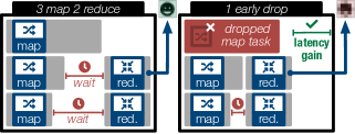
The aim of approximate computing in big data processing (Agarwal et al., 2013; Goiri et al., 2015) is to solve the performance conundrum between latency and accuracy requirements of analysis jobs. Instead of processing all the input data, only a subset of data is chosen to be processed to lower the overall computation demand and reduce latency. Existing systems (e.g., ApproxHadoop (Goiri et al., 2015)) put a significant engineering effort to enable dropping (map) tasks and their assigned input data prior or during execution. Figure 2 illustrates this task dropping strategy on a simple job with 3 map and 2 reduce tasks, with the goal of attaining a given approximation level. In this example, we randomly choose one map task and drop it before its execution. Task dropping saves the overhead of fetching data and avoids the execution of the dropped tasks. Nevertheless, while it reduces the computational demand of jobs, it unavoidably degrades the analysis accuracy. This precision loss depends on both the analysis performed and the data, and can be estimated offline as shown in Section 5.1.

Figure 3. Schematics of differential approximation.

3.2. Architecture of the DiAS prototype

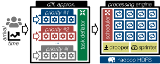
Figure 3 depicts the architecture of DiAS. The key components of DiAS are: (1) a set of job buffers for each priority, indexed by $k\in\{0,\dots,K\}$, (2) the task deflator that determines the approximation level $\theta_{k}$ and sprinting timeout $T_{k}$ for each priority $k$, and (3) the sprinter which temporarily sprints jobs . Higher values of $k$ indicate higher priority. The deflator has two main functionalities: (i) to determine the approximation level and sprinting timeout based on empirical/stochastic models as well as on performance and budget thresholds, and (ii) to dispatch jobs from the priority buffers into the processing engine. We first describe how the deflator dispatches and evicts jobs and derive the analytical models in Section 4.

Upon arrival, jobs are immediately dispatched to the corresponding buffer according to their priorities. Jobs queued at each buffer are processed in a FCFS manner. The task deflator selects the job at the head of the highest non-empty priority buffer, say $k$. This priority-$k$ job with its corresponding approximation level, $\theta_{k}$, is sent to the processing engine, which splits the job into multiple tasks on the cluster. To avoid potential resource waste caused by eviction using preemption, the execution across priority buffers of DiAS is non preemptive. DiAS only dispatches jobs from the head of the buffer to the processing engine when the previous job completes, independent of the priority of newly arrived jobs. Moreover, DiAS assumes that the processing engine is able to drop tasks to achieve the target ratio $\theta_{k}$. We note that as DiAS aims to reshape the job workloads prior to entering the processing engines, the design of DiAS is general and compatible with different processing engines.

For our baseline results with preemption, DiAS also provides the ability to evict jobs from the processing engine. In this case, as soon as any job arrives with a higher priority than the job currently being processed, the job in the engine is evicted back to the head of its buffer and the arriving job is immediately sent in for execution.

In addition, DiAS can leverage computational sprinting to further counter the effects on higher priority jobs stemming from not preempting lower priority ones. If sprinting is enabled, the deflator in parallel to dispatching the job communicates to the sprinter the sprinting timeout $T_{k}$ to use. Once the timeout elapses, the sprinter will temporarily accelerate the execution of the job.

3.3. Implementation

We implement the DiAS prototype in the Go programming language and use Spark as big data processing engine. In addition to priority buffers and the deflator, we also implemented a workload generator and augment Spark with the capability to drop tasks. To deliver the aforementioned functionalities, DiAS is designed to be multi-threaded.

Deflator. The deflator consists of one dispatcher and one monitor thread. When a job completes or a new job arrives, the dispatcher thread selects which job to run and dispatches it using the os.exec library. It does so by first creating a cmd structure and then launches the process with Start(). When evicting jobs, this thread sends the SIGKILL to the process using cmd.Process.Kill(). The monitor thread surveils the running job, collecting its exit status via Wait() and actively relays the completion/eviction of the job to the dispatcher thread using a golang channel.

Sprinter. If sprinting is enabled, the sprinter handles a sprinting timer for each dispatched job and tracks the remaining sprinting budget. When the timer fires, it uses DVFS to temporarily accelerate the job execution by adjusting the frequency of the CPU on the cluster nodes via the cpupower utility. A job is accelerated until either its end or the depletion of the sprinting budget. The sprinting budget is replenished over time using a replenishing rate, e.g., 6 sprinting minutes per hour (AWS, 2019). The timeout is ignored if the job ends sooner.

Dropper. A Spark job typically analyzes a dataset stored as files in HDFS. Each Spark job is translated into a DAG of operations on Resilient Distributed Datasets (RDD) used as input/output. The job execution proceeds in stages (i.e., periods of synchronization points). Each RDD is made of multiple partitions, the number of which indicates the parallelism achievable by Spark, as each partition can be concurrently executed by only one task. The size of a job is thus conventionally defined by the number of RDDs and their partitions (equivalently tasks). Each stage relies on the findMissingPartitions() function to get the number of partitions to be computed. To implement task dropping in Spark, we modify findMissingPartitions() to return only $\lceil n(1-\theta_{k})\rceil$ partitions out of $n$ following the specifications of the deflator.

4. Modeling DiAS

To guide DiAS, we analytically derive the response time distribution offered by the cluster to the incoming multi-task jobs classified in multiple priorities. Jobs are classified in $K$ priorities, where a priority-$k$ job has precedence over jobs in priority levels $l<k$, for $1\leq l,k\leq K$. According to the DiAS architecture, jobs are served in FCFS order and each job seizes all the resources in the cluster (or in the partition used by the corresponding engine) to execute. This can be viewed as a single server queue serving $K$ priority classes. We thus opt to employ the recent method proposed in (Horváth, 2015), which is capable of obtaining the response time distribution and its moments for a fairly general priority queue with $K$ priority classes under both preemptive and non-preemptive scheduling.

One key reason to choose (Horváth, 2015) as the latency model for DiAS is its support for Phase-Type (PH) job processing times (Latouche and Ramaswami, 1999), which is a class of distributions that can capture fairly general behaviours. Further, PH distributions are closed under a number of operations, a feature that we exploit to model the detailed job processing times of concurrent tasks. Instead of using a given distribution to model the job processing time, we resort to a bottom-up approach and build a more detailed view at the task level or wave levels. For a description of waves and their role in job execution see Section 4.2 below. We thus exploit PH distributions to capture details of tasks and waves (i.e., no. of waves =$\lceil{\frac{no.\,tasks}{no.\,slots}}\rceil$) within the job processing time and build upon recent results on priority queues with PH components (Horváth, 2015).

Background on the MMAP[$K$]/PH[$K$]/1 priority queue. Horváth (Horváth, 2015) analytically derived the latency distribution for an MMAP[$K$]/PH[$K$]/1 priority queue, where processing times follow PH distributions, differentiated for the $K$ job classes, and arrivals follow a Marked Markovian Arrival Process (MMAP) with $K$ different streams (Latouche and Ramaswami, 1999), one for each priority class. This class of arrival processes can capture fairly general behaviors, including correlations among arrival streams or general inter-arrival times. The parameters of an MMAP are $K+1$ $m_{a}\times m_{a}$ matrices $(\bm{D}_{0},\bm{D}_{1},...,\bm{D}_{K})$, where $\bm{D}_{k}$ holds the transition rates for class-$k$ jobs, and $\bm{D}_{0}$ ensures that the matrix $\bm{D}=\sum_{k=0}^{K}\bm{D}_{k}$ is the generator of a Markov chain. The simplest non-trivial example is the marked Poisson arrival process, where $m_{a}=1$, $\bm{D}_{k}=\lambda_{k}$, which is the arrival rate of class-$k$ jobs, and $\bm{D}_{0}=-\sum_{k=1}^{K}\lambda_{k}$.

Table 1. Summary of notation.

Symbol	Definition
$C$	Number of computing slots
$N_{m}^{k}$	Max. number of map tasks in a priority-$k$ job
$N_{r}^{k}$	Max. number of reduce tasks in a priority-$k$ job
$p_{m}(t)$	Prob. that a priority-$k$ job has $t$ map tasks
$p_{r}(u)$	Prob. that a priority-$k$ job has $t$ reduce tasks
$1/\mu_{m}^{k}$	Mean exec. time for map tasks in a priority-$k$ job
$1/\mu_{r}^{k}$	Mean exec. time for reduce tasks in a priority-$k$ job
$1/\mu_{o}^{k}$	Mean setup time for a priority-$k$ job
$1/\mu_{s}^{k}$	Mean shuffle time for a priority-$k$ job
$\theta_{m}^{k}$	Approximation ratio for map tasks in a priority-$k$ job
$\theta_{r}^{k}$	Approximation ratio for reduce tasks in a priority-$k$ job
$\mathcal{O}$	Overhead stage
$\mathcal{M}_{t}$	Map stage with $t$ map tasks left to process
$\mathcal{S}$	Shuffle stage
$\mathcal{R}_{u}$	Reduce stage with $u$ map tasks left to process

Assumptions and notations on the cluster and approximate/sprinting jobs. We assume the cluster, or the allocated partition, is composed of $C$ computing slots. Priority-$k$ jobs have $n_{m}^{k}$ map and $n_{r}^{k}$ reduce tasks, both of which are discrete random variables with minimum value 1 and maximum value $N_{m}^{k}$ and $N_{m}^{k}$, respectively. On average, the time to execute a map task is $1/\mu_{m}^{k}$ and to execute a reduce task is $1/\mu_{r}^{k}$. In addition, the job execution may include an initial setup time that lasts $1/\mu_{o}^{k}$ time on average, and an intermediate shuffle stage that requires on average $1/\mu_{s}^{k}$ time. We note that, when sprinting is enabled, the service rates can be approximately captured by the effective sprinting rates as a weighted average of the sprinted and non-sprinted execution times per task and class $k$. Predicting these rates is complex (Morris et al., 2018). We assume that the effective sprinting rates are provided by an oracle for each class $k$ and timeout value. Moreover, as the number of executors available is less than the number of parallel tasks and executors comprise multiple cores, each executor concurrently executes multiple tasks. Hence, our current approach sprints all available cores at the same time which is beneficial for applications consisting of tasks with equal workloads. We leave the estimation of effective sprinting rate for complex sprinting policies as future work. Table 1 summarizes the notation.

4.1. Task-level Model

For priority-$k$ jobs, we set the task drop ratio to $\theta_{m}^{k}$ for map tasks and to $\theta_{r}^{k}$ for reduce tasks. The effective number of map and reduce tasks is thus ${\bar{n}_{m}^{k}=\lceil n_{m}^{k}(1-\theta_{m}^{k})\rceil}$ and ${\bar{n}_{r}^{k}=\lceil n_{r}^{k}(1-\theta_{r}^{k})\rceil}$. Moreover, as the number of tasks is a random variable, we let $p_{m}^{k}(t)$ and $p_{r}^{k}(u)$ be the probabilities that a priority-$k$ job has $t$ map and $u$ reduce tasks, where $1\leq t\leq N_{m}^{k}$ and $1\leq u\leq N_{r}^{k}$. From this point on, we drop the super-index $k$ for clarity, but the definitions apply to all job priorities making use of the appropriate index.

With the above definitions we can extend the model in (Pérez et al., 2017) to incorporate the overhead $\mathcal{O}$ and shuffle stages $\mathcal{S}$, as well as to allow for a variable number of tasks. We thus let the processing phase $i$ keep track of the job current execution step, where: (i) $i=\mathcal{O}$indicates the job is in the initial setup (overhead) stage; (ii) $i=\mathcal{M}_{t}$indicates that $t$ map tasks remain to be completed, for $1\leq t\leq\bar{N}_{m}$; (iii) $i=\mathcal{S}$indicates the job is in the intermediate shuffle stage; (iv) $i=\mathcal{R}_{u}$indicates that $u$ reduce tasks remain to be completed, for $1\leq u\leq\bar{N}_{r}$. All jobs start in stage $\mathcal{O}$ and their evolution is determined by the transition rates from phase $i$ to the next phase $j$, $f(t,j)$, defined as:

(1) $$f(i,j)=\begin{cases}\mu_{o}p_{m}(t),&i=\mathcal{O},j=\mathcal{M}_{\bar{t}},\\ C\mu_{m},&i=\mathcal{M}_{t},j=\mathcal{M}_{t-1},t\geq C,\\ t\mu_{m},&i=\mathcal{M}_{t},j=\mathcal{M}_{t-1},2\leq t<C,\\ \mu_{m},&i=\mathcal{M}_{1},j=\mathcal{S},\\ \mu_{s}p_{r}(u),&i=\mathcal{S},j=\mathcal{R}_{\bar{u}},\\ C\mu_{r},&i=\mathcal{R}_{u},j=\mathcal{R}_{u-1},u\geq C,\\ u\mu_{r},&i=\mathcal{R}_{u},j=\mathcal{R}_{u-1},1\leq u<C,\\ \end{cases}$$

where ${\mathcal{R}}_{0}$ denotes the end of all reduce tasks and the job completion.

In (1) the first row corresponds to a transition from the initial setup stage $\mathcal{O}$ to the map stage for a job with $t$ map tasks, i.e., it actually starts with $\bar{t}$ tasks due to early drop. The next two rows show that the maximum parallelism is $C$ and that tasks finish one by one until the map stage is completed. The next transition is to the shuffle stage $\mathcal{S}$, after which the job moves on to the reduce stage, where, after dropping, a total of $\bar{u}$ tasks must be executed if the job has $u$ reduce tasks. Since $N_{m}$ and $N_{r}$ are the maximum number of map and reduce tasks, the phase space is $\mathcal{P}=\{\mathcal{O},\mathcal{M}_{\bar{N}_{m}},\dots,\mathcal{M}_{1},\mathcal{S},\mathcal{R}_{\bar{N}_{r}},\dots,\mathcal{R}_{1}\}$, and we can build a transition matrix $\bm{F}$ with entries $f(i,j)$ in (1) for $i,j\in\mathcal{P}$. Further, we define the vector $\phi=[1\quad\bm{0}]$ as the initial phase distribution, where 1 indicates that all jobs start processing in phase $i=\mathcal{O}$. The pair $(\phi,\bm{F})$ is thus a PH representation (Latouche and Ramaswami, 1999) of the job processing time with ${N_{m}+N_{r}+2}$ phases.

4.2. Wave-level Model

Whereas the just described model is very detailed in considering the evolution at the task level, it assumes that task execution times follow an exponential distribution. Generalizing this assumption at the task level is very challenging as it would require keeping track of individual tasks separately. We thus take a different approach. We observe that tasks tend to have fairly similar execution times (Morris et al., 2018), leading to an execution in waves. For instance, a job composed of 40 tasks executing in a cluster with 20 computing slots will start with a first wave of 20 tasks executing in parallel. If these tasks have fairly similar execution times, they will finish close to each other, allowing the next 20 tasks to execute almost at the same time, making up a second wave. This wave-level model captures this behavior, having the job processing time as a sequence of waves, each with a wave execution time.

Given $C$ computing slots and a job made up of $t$ and $u$ map and reduce tasks, respectively, its effective number of map and reduce waves are $\bar{w}_{m}=\lceil\bar{t}/C\rceil$ and $\bar{w}_{r}=\lceil\bar{u}/C\rceil$, respectively. Recall that $\bar{t}=\lceil t(1-\theta_{m})\rceil$ is the effective number of map tasks to execute once a task drop ratio $\theta_{m}$ is applied. Since waves are consecutive, we can model the execution time of the $d$-th map wave as a PH distribution with $v_{m(d)}$ phases and parameters $(\alpha_{m(d)},A_{m(d)})$, avoiding the exponential assumption and allowing for fairly general behaviors. Moreover, we allow each wave to have a potentially different execution time, as we also observed in our experiments with state-of-the-art execution engines, e.g., Spark. We similarly let the $d$-th reduce wave have a PH distribution with $v_{r(d)}$ phases and parameters $(\alpha_{r(d)},A_{r(d)})$. Also, let the initial setup stage have $v_{o}$ phases and parameters $(\alpha_{o},A_{o})$, and the intermediate shuffle stage have $v_{s}$ phases and parameters $(\alpha_{s},A_{s})$. We further define the exit rate vector $a_{x}=-A_{x}\bm{1}$ for $x$ representing any of the stages considered. Since the sum of independent PH random variables is also PH (Latouche and Ramaswami, 1999), we represent the job processing time as a PH distribution with $v=v_{o}+\sum_{d=1}^{w_{m}}v_{m(d)}+v_{s}+\sum_{d=1}^{w_{r}}v_{r(d)}$ phases and parameters $(\alpha,A)$.

For clarity, consider the case where $w_{m}=w_{r}=2$, i.e., both map and reduce stages are composed of 2 waves of execution. The transition matrix $A$ of the job processing time for this case is:

where $q_{m}(d)$ and $q_{r}(d)$ are the probabilities that a job requires $d$ waves of execution in the map and reduce stages, respectively. These can be computed as

$$q_{m}(d)=\sum_{\bar{t}=(d-1)C+1}^{dC}\ \sum_{t:\lceil t(1-\theta)\rceil=\bar{t}}p_{m}(t),$$

where the inner sum accounts for the probability that a job has $\bar{t}$ effective map tasks after dropping, and the outer sum accounts for all cases where the $\bar{t}$ effective tasks can be executed in $d$ waves. Finally, the initial probability vector can be written simply as $\alpha=\begin{bmatrix}\alpha_{o}&0\end{bmatrix},$ since all jobs start in the setup stage, completing the PH representation of the job processing time at the wave level.

4.3. Validation

Figure 4. Validation of job processing times for different datasets and priorities.

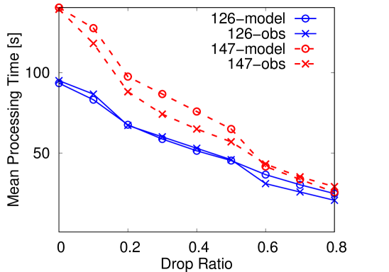
We now illustrate the results obtained with the model against those observed experimentally. We first consider two different datasets, for which we obtain map and reduce task execution times from a profiling run. The details of experiments can be found in Section 5. We also collect samples of the overhead times, which we have observed to be dependent on the data size. To keep profiling at a minimum, we collect overhead times from two configurations only: one where no task drop is performed, and one where 90% of the tasks are dropped, which is the maximum drop ratio we consider. Then, for a given drop ratio we determine the associated mean overhead time by a simple linear interpolation between these two extreme scenarios. Figure 4 shows the observed job execution times (x marks) for several drop ratios and two different datasets. It also shows the predicted job execution times (o marks) obtained with the model from estimations of the task execution time, the overhead, and setting the task drop ratio. The results show that the model accurately predict the job processing time as a function of the drop ratio, with mean errors of 11.1% and 7.8% for the two datasets shown. Similar results hold for other datasets but we omit them in the interest of space.

We now employ the model to predict the job response time, parameterizing the model with the same information as above: mean task execution time and overhead. Also, we set the arrival rate to achieve an 80% cluster utilization and test several values for the drop ratio. Note that for low loads the response times are similar to the processing times, which we have shown above to be accurately predicted by the model. We are thus interested in testing a high load scenario where the model must be able to predict well both the processing and waiting times. Further, we let high- and low-priority jobs process different datasets, such that the average low-priority job size is 2.36$\times$ larger (1117MB and 473MB, respectively), and the ratio between low- and high-priority jobs is set to 9 (i.e., more low-priority jobs). This setup is similar to the ones used in the experimental section. Figure 5 shows the observed and predicted mean response times for both low- and high-priority jobs. The model is clearly able to follow the decrease in response times as the drop ratio increases, with an average error of 18.7%.

Figure 5. Validation of response times for different datasets and priorities.

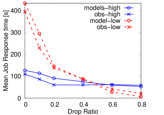
We can therefore employ the model to determine whether a certain configuration under a given workload can achieve a preset latency objective. In fact, the model predictions can be used to determine a minimum value for the drop ratio, such that the latency degradation on the high-priority jobs is kept limited. Together with a constraint on the accuracy error, it is possible to provide the user with latency-accuracy pairs for feasible drop ratios, each of which presents a different tradeoff.

5. Evaluation

This section presents our extensive evaluation of the DiAS prototype atop Spark engine. We compare it against priority systems, being preemptive or non-preemptive without approximation and sprinting. The specific question we answer in this section is: given the accuracy requirement of multi-priority jobs, how much improvement can be obtained on the average/tail response time of low priority jobs without any resource waste and degradation of high priority jobs? We first describe our experimental setup, the configuration used for Spark and the workload details. Specifically, we focus on big data applications of text and graph analytics. The number of priorities is defined based on the characteristics of Google trace which has 12 priorities but is is dominated by two to three classes that account for 89% of all tasks  (Çavdar et al., 2014). Therefore, although our proposed methodology can easily be extended to larger number of priorities, we will focus on the scenario of two and three priorities. We first evaluate the design of differential approximation (§5.2), followed by the full fledged design of DiAS - combining differential approximation and sprinting. While the differential approximation improves the low priority jobs at a marginal degradation of the high priority jobs, the complete DiAS (§5.3) can improve the performance of both priorities, compared to standard preemptive and non-preemptive systems.

5.1. Experimental Setup and Workloads

Spark processing engine. We rely on Spark v2.1 and a cluster with one master and ten workers. Each worker uses 2 CPU cores, and 4 GB memory. Our machines consist of Dell PowerEdge R330 servers equipped with Intel Xeon E3-1270 v6 CPU, 64 hyper-threaded cores and 128 GB memory, interconnected by a 10G Ethernet switched network on a star topology. To store the data, we deploy HDFS (v2.8.0), using one namenode and three datanodes (hdf, 2019).

Figure 6. Impact of task dropping on accuracy loss: the trend of mean absolute error.

Text analysis jobs. We deploy jobs that perform text analysis on XML data dumps collected from 164 StackEchange websites (sta, 2019) each dedicated to a different topic. The goal of the analysis is to find the popularity of different words in different topics by first parsing the XML to extract the posts of users followed by counting the frequency of words. Each Spark job processes one such data set. To take advantage of the 20 cores in our Spark cluster, following Spark’s tuning suggestions (Spa, 2019), we split each dataset into 50 RDD partitions. Accordingly, Spark processes RDDs in multiple waves. Jobs arrive following an exponentially-distributed inter-arrival time and enqueued before being dispatched to the Spark engine. We tune the arrival rate to obtain a 80% (50%) system utilization based on offline profiling of our scenario. The job response time is thus composed of the queueing time and processing time. The main metrics of interests include the average and tail response time, i.e., $95^{th}$, for each priority.

Graph analysis jobs. We run the triangle count algorithm implemented by the Spark’s graphx (gra, 2019) library. The input dataset consists on the public Google web graph (Leskovec et al., 2009), with 875’713 nodes and 5’105’039 edges. There are three types of jobs: (1) to build the edge RDD, (2) to build the vertex RDD, and (3) for the triangle count itself, composed by six ShuffleMap stages and one Result stage.

Differential approximation. We specifically consider scenarios of two and three levels of job priorities, with different characteristics, i.e., job sizes, arrival ratios across priorities, and overall system load. As for the accuracy loss, we compute the relative errors offline under different task dropping ratios as shown in Figure 6. The mean absolute error in percentage increases sub-linearly with dropping ratios. When dropping 10% or 20% of map tasks, the relative errors are roughly 8.5% and 15%, respectively. Therefore, in the remainder of our evaluation section, we set the acceptable relative error to 0 for high-priority jobs and to 8.5%, 15% and 32% for lower-priority jobs. This corresponds to evaluating the latency impact of DiAS that drops 10%, 20% or 40% of tasks in lower-priority jobs.

Figure 7. Mean (solid bars) and tail (shaded bars) latency improvement of two differential approximation variations on a two-priority system. $P$: preemptive, absolute values. $NP$: non-preemptive. $NP$, $DA_{(0,100)}$, and $DA_{(0,20)}$ as relative difference to $P$.

(a) Equal job sizes	(b) Much more high-priority jobs	(c) 50% system load

Figure 8. Sensitivity analysis of differential approximation on mean (solid bars) and tail (shaded bars) latencies by changing the ratios between high and low priority jobs: sizes, arrival rates, and the overall system utilization.

Differential sprinting. We use DVFS as the sprinting mechanism to change the speed of the CPU. The CPU clock frequency is initially set to 800MHz old and temporarily increase it to 2.4GHz old when sprinting. These frequencies were defined based on the limits supported by the machines used, which also corresponds to a common setup (fre, 2019). Sprinting reduces the execution time of high priority jobs by up to 60%, but increases the servers power consumption by 1.5x, from 180W to 270W. In the following, we consider two types of energy budgets: (1) limited sprinting, to sprint only 35% of the execution time of high priority jobs, and (2) unlimited sprinting, to sprint high priority jobs for their whole duration. Under limited sprinting high priority jobs sprint after 65 seconds. Under unlimited sprinting they sprint as soon as they are dispatched.

Resource waste. With DiAS, differential approximation and sprinting levels are applied on different priorities and lower-priority jobs are never evicted upon arrival of a higher-priority job. As a result, machine time is never wasted on reprocessing evicted jobs compared to a preemptive priority system. We define the resource waste as the percentage of machine time used to re-process evicted jobs compared to the total processing time.

5.2. Differential Approximation

5.2.1. Two-Priority System

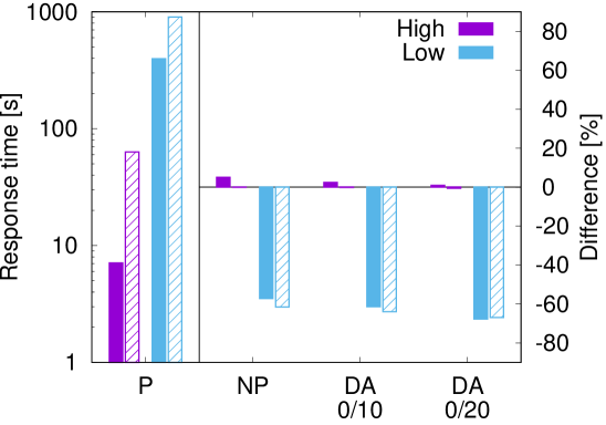
We first show the effectiveness of differential approximation on a reference setup, highlighting the difference of mean and $95^{th}$ latency for both high- and low-priority jobs when compared to a preemptive and a non-preemptive priority system denoted as $P$ and $NP$, respectively. The three key parameters in the reference setup are: (i) the ratio between low- and high-priority jobs is 9 to 1, (ii) the average sizes of low- and high-priority jobs are 1117MB and 473MB, respectively, (iii) and the average system load is 80%. The parameters are set as close as to the workload characteristics of Google trace (Wilkes, 2011). Figure 7 summarizes the absolute results of the preemptive priority setup, and its relative difference compared to a non-preemptive priority setup, $DA_{(0,10)}$ and $DA_{(0,20)}$. The subscript pair of $DA$ denotes the task dropping ratio for high- and low-priority respectively. We use solid bars for the mean latency, while shaded bars are for the $95^{th}$ percentile latency. The resource waste is roughly 4% with the preemptive priority policy.

Under $P$, the mean latency of high-priority is better than the low-priority job. This stems from the unbalance in the queueing times: 0.03s versus 310s on average for high- and low-priority jobs, respectively. This difference is smaller for the $95^{th}$ percentile. When using the $NP$ model, where preemption of low-priority jobs is not allowed, the performance of low-priority jobs improves roughly by 20% at the cost of increasing the latency of high-priority jobs by 80%. This is because high-priority jobs have to wait for the low-priority jobs in execution to finish before getting served. In contrast, $DA_{(0,20)}$ can significantly improve the performance (roughly 65%) of both mean and tail latency of low-priority at only a marginal (10%) increase in the mean latency of high-priority jobs and an accuracy loss for low-priority jobs of 15%.

We further consider a use case scenario where it is possible to tolerate a 30% accuracy loss for low-priority jobs while maintaining the latency of high-priority jobs under 100ms with no accuracy loss. The task deflator consults the results in Figure 6 to determine the maximum drop ratios to attain an accuracy target of 0% and 30% for high- and low-priority jobs, respectively. Likewise, the deflator runs the DiAS model (Section 4) and determines that a 20% drop ratio for low-priority jobs is already within the 100ms limit for the high-priority mean latency (as Figure 5 shows). We can thus choose to employ $DA_{(0,20)}$ to hold both accuracy and latency constraints, as confirmed by the experimental results in Figure 7. This selection can be easily automated by assigning weights to the latency and accuracy targets to select among the feasible drop ratios.

5.2.2. Sensitivity Analysis

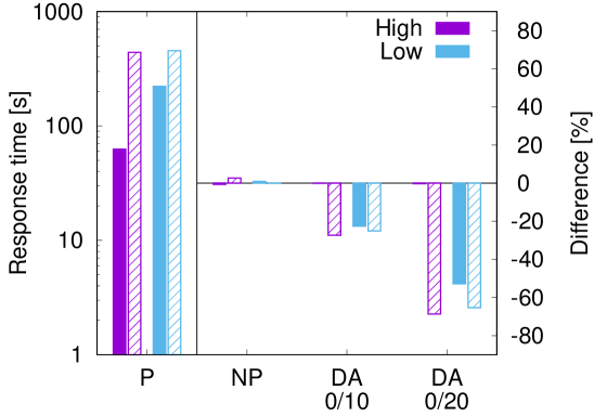
Our sensitivity analysis of differential approximation fiddles with following parameters in the reference setup one at a time: (i) high- and low-priority jobs of same size, (ii) ratio between low- and high-priority jobs set 1 to 9, and (iii) a total arrival rate resulting in a 50% system load. Figure 8 summarizes the results for these three scenarios. Due to the rich information embedded in the figure, we focus on comparing the latency gains of differential approximation between the reference and new setup.

Similar job size for both priorities. Comparing Figure 8 (a) and Figure 7, the latency gain of differential approximation is significant, i.e., for low-priority up to 80%. High-priority jobs improves too: both their mean and tail latencies have better improvement than the reference system. This can be explained by the fact that high-priority jobs have shorter waiting time here than in the reference system. In a non-preemptive setting, being in $NP$ or $DA$, the maximum amount of queueing time for an arriving high-priority job is a single execution of low-priority job, assuming the high-priority queue is empty. Hence, smaller the low-priority jobs, better the gain of differential approximation used in the non-preemptive setup.

Relatively increased high- to low-priority job ratio. Comparing Figure 8 (b) and Figure 7, the latency gain of differential approximation is worse. Both the mean and tail latency of high-priority increase considerably. Though the average latency gain of low-priority remains the same as the reference case, the tail latency gain decreases from 60% to 20%. As differential approximation only applies approximation techniques on low-priority jobs which account for 10% of the total jobs, its effectiveness is limited. Hence, in the scenario of dominant high-priority jobs, one shall activate approximation for both priorities.

Relatively low system loads. Comparing Figure 8 (c) and Figure 7, the latency gain of $DA_{(0,10)}$ is slightly worse, but $DA_{(0,20)}$ maintains a similar gain as the reference setup. Further, there is almost no performance degradation from preemptive to non-preemptive system, shown by the results of $NP$. When the system load is low, e.g., 50%, there is no difference between preemptive and non-preemptive priority systems because the engine is rarely occupied when higher-priority jobs arrive. The gain of $DA_{(0,20)}$ on low-priority jobs is thus mainly attributed to the reduction of processing time, instead of queueing time. Moreover, the difference between $DA_{(0,10)}$ and $DA_{(0,20)}$ can be explained by the fact that dropping 20% of tasks reaches the critical mass to drop an entire wave. Overall, thanks to flexible approximation levels and stochastic models of deflator, differential approximation can effectively tradeoff analysis accuracy for improved mean/tail latencies of high/low-priority jobs, against complex system and workload dynamics.

5.2.3. Three-Priority System

Figure 9. Differential approximation on three-priority system: relative difference in mean (solid bars) and tail (shaded bars) latency against preemptive priority ($P$).

We demonstrate the performance gains for differential approximation on a system with three priorities: high, medium and low (Figure 9). The total arrival rate is 2.3 jobs/min with rate ratio of high-medium-low priority of 1-4-5, resulting in roughly 80% system load. For drop rates, we use $DA_{(0,10,20)}$ and $DA_{(0,20,40)}$: the former introduces 8.5(15)% accuracy loss for medium(low)-priority jobs, and the latter introduces 15(32)% accuracy loss for medium(low)-priority jobs according to Figure 6.

Similar to the two-priority scenario, we use the mean/tail latency of the preemptive priority setup as comparison baseline. The resource waste under $P$ is roughly 16%. The remaining three setups in Figure 9 incur in zero resource waste, due to their non-preemptive nature. In terms of latency improvement, differential approximation is able to significantly reduce the tail latency for all three priorities by up to 60%. Differential approximation reduces the average latency more for low-priority than medium-priority. However, such improvement of differential approximation comes at the cost of slightly higher average latency of high-priority jobs and accuracy loss of low- and medium-priority jobs. In this particular setup, $DA_{(0,10,20)}$ appears to achieve the most moderate tradeoff among accuracy/latency for high/lower-priority jobs.

Figure 10. Differential approximation on triangle count: relative difference in mean (solid bars) and tail (shaded bars) latency against preemptive priority scheduler ($P$).

(a) Latency: limited sprinting	(b) Latency: unlimited sprinting	(c) Energy comparison

Figure 11. Complete DiAS on triangle count: latency and energy improvement against the preemptive priority scheduler (P). In (a) and (b), the mean and tail latency are in solid bars and shaded bars, respectively.

5.2.4. Differential Approximation on Triangle Count

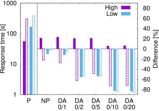
We further illustrate the gains of differential approximation when the computation requires several map and reduce stages. Specifically, we run the triangle count algorithm implemented in graphx library in Spark. Task dropping in this case is performed on every ShuffleMap stage, for which we consider drop ratios {1,2,5,10,20} for the low-priority jobs. The total effective drop ratio is thus the result of applying the stage drop ratio in each stage.

Figure 10 displays the gains obtained with differential approximation with respect to preemptive and non-preemptive scheduling. Clearly, with fairly limited task dropping ratios (5-10%) differential approximation is able to reduce the mean latency of low-priority jobs by over 50%. Moreover, differential approximation reduces by a similar factor the tail latency of both high and low-priority jobs.

5.3. Differential Approximation and Sprinting

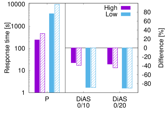
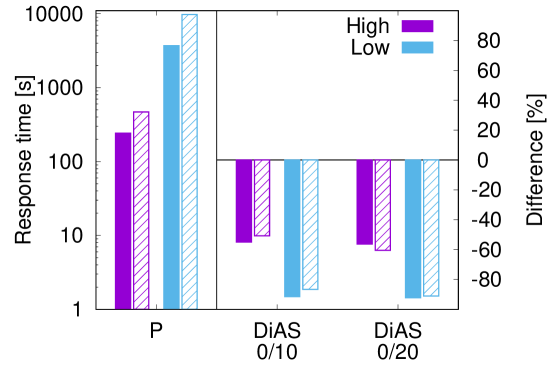
Finally, we evaluate the complete design of DiAS, applying different CPU sprinting on the high priority jobs and approximation on the low priority jobs. We consider graph analytics jobs, which has high and low priorities of the same job size with a ratio of 3 to 7. We experiment the CPU sprinting policy under two different energy budgets resulting in two different scenarios. In the first scenario, i.e., limited sprinting shown in Figure 11 (a), we consider a sprinting budget of 22kJ which roughly limits the jobs to run in high frequency only for 35% of their execution time based on timeout. In the second one, i.e., unlimited sprinting shown in Figure 11 (b), we set the budget high enough such that the high-priority jobs run at high frequency throughout their whole execution time. We use a non-sprinted $P$ system as the baseline for the ease of comparison.

Latency gain. The complete DiAS of differential approximation and sprinting shows promising performance. First, the average and tail latency of both priorities improve under limited and unlimited sprinting budgets, ranging between 35% to 90%. Overall, the latency gain is more prominent for the tail latency, low-priority jobs, and unlimited sprinting. In terms of absolute comparison, the improvement for low-priority jobs is around 90%, whereas high-priority is between 40-60% depending on the sprinting budget. We stress that few cases with increased average latency of high-priority jobs observed in Section 5.2 are effectively countered by enabling differential sprinting. The performance gains are therefore more consistent for both tail and average latency, compared to the approximation-only results.

Despite the focus of sprinting being on high-priority jobs, the response times of low-priority jobs are also indirectly improved. When compared to differential approximation only, the average response time of $\textsc{DiAS}_{(0,20)}$ increases up to 55% for high-priority jobs but also up to 40% for low priority jobs. Similarly, for $\textsc{DiAS}_{(0,10)}$ the increase goes up to 50% and 53% for high- and low priority jobs, respectively. That is, by reducing the processing time of high-priority jobs, the queueing time of low-priority jobs is reduced, directly affecting the response time for both types.

Latency decomposition. To unveil the exact performance advantage of DiAS, we zoom into the performance of the limited sprinting case and present the average queueing and execution times for high- and low- priority jobs in Table 2. We also apply the same sprinting policy on the non-preemptive system, termed $NPS$. Due to sprinting, the execution times of high-priority jobs are lower than the low-priority jobs by at least 25%. Because of the 20% task dropping in $\textsc{DiAS}_{(0,20)}$, the average execution time of the low-priority jobs is the lowest among the three policies, i.e., around $131$ seconds. The percentage of time that low-priority jobs occupy the system thus reduces, avoiding longer waiting time for both high- and low-priority jobs. As such, the queueing times for both high- and low-priorities are lower than $NPS$ and $\textsc{DiAS}_{(0,10)}$.

Table 2. Average queueing and execution times of high- and low-priority jobs under sprinted non-preemptive scheduling (NPS), $\textsc{DiAS}_{(0,10)}$ and $\textsc{DiAS}_{(0,20)}$.

	NPS		$\textsc{DiAS}_{(0,10)}$		$\textsc{DiAS}_{(0,20)}$
	Queue [s]	Exe.[s]	Queue [s]	Exe.[s]	Queue [s]	Exe. [s]
High	70.6	99.8	70.0	100.2	55.1	99.4
Low	378.9	148.5	286.42	139.0	238.0	131.1

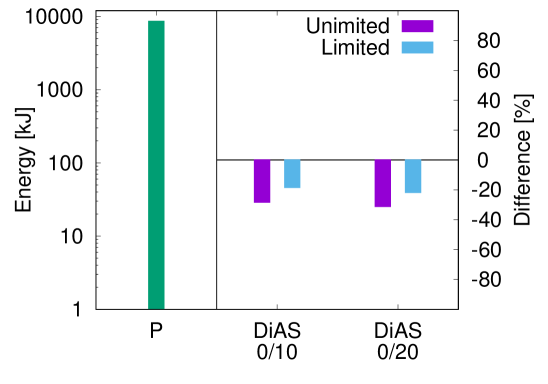
Energy gain. In Figure 11(c), we summarize the normalized energy consumption of DiAS against the $P$ policy. For both unlimited and limited sprinting, we temporarily increase the CPU frequency for high-priority jobs. One would expect a slightly higher energy consumption, compared to the no-sprinting baseline. Surprisingly, for both unlimited and limited cases, DiAS reduces the overall energy consumption. The energy reductions stemming from differential sprinting alone for the limited and unlimited budgets are around 15% and 26%, respectively. We explain this result by the significant reduction in execution times that outweighs the power increase during sprinting.

The energy gain of DiAS can also be amplified by the approximation ratios, i.e., $\textsc{DiAS}_{(0,10)}$ and $\textsc{DiAS}_{(0,20)}$. With unlimited sprinting the gain increase to 28.2% and 31% for $\textsc{DiAS}_{(0,10)}$ and $\textsc{DiAS}_{(0,20)}$, respectively. Similarly, for limited sprinting we observe 18.3% and 21.6%. Higher reductions are observed for higher drop rates, as dropping reduces the computational load on the cluster. Overall, the design of combining differential approximation and differential sprinting can improve both the latency of both priorities and energy consumptions across diversified systems scenarios.

We suggest the following procedure to determine the static threshold used in the algorithm. To utilize the proposed models to predict the performance, one needs to first obtain the input parameters of the proposed models through workload profiling, that quantifies the relationship between file size and execution time under a constant CPU frequency. Then, one can exhaustively search through different combinations of dropping ratios, priorities, and frequency thresholds. Our proposed models can estimate the latency of such large combinations quickly. The values that optimize the tradeoff are then selected for a given set of workloads. We note that such searching procedure needs to be evoked upon every workload changes. DiAS considers a scenario where the workload set is given and hence only consider the static threshold.

6. Related Work

A plethora of state-of-the-art systems developed novel priority-aware or approximation/sprinting-enabled processing platforms. We particularly highlight those focused on managing priority, approximation frameworks and sprinting strategies for Spark-like applications. Moreover, we summarize efforts on computational sprinting and modelling that address the challenging question – latency distribution for multi-priority jobs composed of multiple parallel tasks.

Priority systems. Characterization studies (Chen et al., 2012; Çavdar et al., 2014; Rosà et al., 2015a) on production big data systems show that multi-task jobs are associated with multiple priorities and exhibit diverse workload characteristics (Chen et al., 2012). To ensure the performance of (particularly high) priority jobs, the scheduler evicts low-priority jobs to make resource available for high priority ones, resulting in a significant resource waste (Çavdar et al., 2014) and latency penalty on the low priority jobs (Rosà et al., 2015a). Indeed, modern big processing engines, e.g., Hadoop (had, 2019) and Spark (Spa, 2019), also support multi-priority job scheduling. For instance, Hadoop’s fair scheduler (Fai, 2019) can assign different weights on different workloads to achieve soft priority, i.e., higher (lower) weights on higher (lower) priority. Mesos (Hindman et al., 2011) is a cluster manager that support priorities across and within multiple processing engines with a focus on fairness. Omega (Schwarzkopf et al., 2013) is a two-level priority scheduler designed for large-scale system. Recognizing the need of evictions in priority systems, Natjam (Cho et al., 2013) develops novel job and task eviction policies for a scenario of two priorities that have different deadlines. DiAS proposes an orthogonal solution that alters the jobs resource demands and processing speeds for different priorities, rather than a novel scheduling approach of tasks or jobs.

Approximation big data engines. To process vast and fast amount of data influx, novel approximation-enabled systems are designed to meet the dual objectives of accurate analysis and resource efficiency. In the context of MapReduce paradigm, statistical sampling theory is commonly applied to selectively process a subset of data either at the level of input block (Agarwal et al., 2013) or task (Krishnan et al., 2016), before or after the execution starts. BlinkDB (Agarwal et al., 2013), an approximate query processing framework, provides accuracy guards in short response times by leveraging statistical sampling theory to choose the inputs. ApproxHadoop (Goiri et al., 2015) develops a two-stage sampling strategy for Hadoop (had, 2019) by either dropping the tasks or amount of data per tasks, so as to minimize the overhead of data accessing. To overcome the accuracy loss of sampling, IncApprox (Krishnan et al., 2016) combines the task sampling and incremental computing, i.e., memorizing intermediate historical result. Grass (Ananthanarayanan et al., 2014) is a scheduler that prioritizes jobs with higher approximation level over lower levels for approximate analytics engine.

While approximate big data engines effectively trade accuracy for the latency target and resource efficiency, they only consider single-priority scenarios and often overlook the latency models of complex dependency of jobs arrival.

Computational sprinting. Computational sprinting enables bursts of peak processing in systems limited by dark silicon. Sprinting mechanisms exist nowadays at all system levels, from transistors and processors (Rotem et al., 2012), to computer systems (Komoda et al., 2013), and datacenters (Zheng and Wang, 2015). Sprinting policies decide when and what to sprint, e.g., phases within job executions (Zhang and Hoffmann, 2016) and particular queries  (Jeon et al., 2016). Several approaches have been explored in the single priority scenario, from simple heuristics (Hsu et al., 2015), to queueing (Qiu et al., 2016) and machine learning (Morris et al., 2018) models. DiAS extends the sprinting policies with multi-priority scheduling and approximation schemes such that the performance of all priorities can be improved.

Stochastic models for multi-priority jobs. Modeling the latency for multi-priority jobs is a long standing challenge by itself because of the complex workload dynamics across jobs and the interdependency among tasks. For priority systems, modeling studies can be categorized into single vs. multi-server setus, preemptive vs. non-preemptive, and resume vs. non-resume under preemptive scheduling.  (Harchol-Balter et al., 2005; Wierman et al., 2006) employ matrix analytics method to analyze the jobs average latency in the non-preemptive multi-server system, whereas (Sleptchenko et al., 2005) focus on the state probabilities of preemptive multi-server systems. Horváth (Horváth, 2015) derives the latency distribution in both preemptive and non-preemptive setting for single server system. Jelenkovic (Jelenkovic and Skiani, 2014) derives the stability conditions for non-resume preemptive systems, highlighting the high risk of instability.

The stochastic model in DiAS not only captures the entire distribution of latency for multi-priority and multi-task jobs but also further facilities the optimization of differential approximation and sprinting for real system deployment.

7. Concluding Remarks

We propose a novel design of differential approximation and sprinting, DiAS, to trades off the accuracy and additional sprinting capacity for improving the efficiency of big data engines, i.e., reduction of mean/tail latency without resource waste. The design of DiAS is general, i.e., supports different types of analyses and multiple priorities, and compatible with existing MapReduce based processing engines that provide approximation mechanisms, e.g., task dropping, and dynamic frequency scaling. We derive stochastic models to guide the control of approximation and sprinting levels of DiAS. We implement the prototype of DiAS atop of Spark, with examples of text and graph analytics. Our extensive evaluation results show that DiAS consistently reduces the mean/tail latency of both low- and high-priority jobs (by up to 90% and 60%, respectively) at roughly 15% relative error in the accuracy of low-priority jobs and more than 20% energy reduction, compared to the state-of-art preemptive scheduler.

References

- (1)
- had (2019) 2019. Apache Hadoop. http://hadoop.apache.org/.
- Spa (2019) 2019. Apache Spark. http://spark.apache.org/.
- AWS (2019) 2019. AWS burstable EC2 Instances. https://aws.amazon.com/blogs/aws/low-cost-burstable-ec2-instances.
- gra (2019) 2019. GraphX. https://spark.apache.org/graphx/.
- Fai (2019) 2019. Hadoop Fair Scheduler. https://hadoop.apache.org/docs/r1.2.1/fair_scheduler.html.
- hdf (2019) 2019. HDFS Architecture Guide. https://hadoop.apache.org/docs/r1.2.1/hdfs_design.html.
- fre (2019) 2019. Property: TDP down frequency. https://en.wikichip.org/wiki/Property:tdp_down_frequency.
- goo (2019) 2019. SNAP: Network datasets: Google web graph. https://snap.stanford.edu/data/web-Google.html.
- sta (2019) 2019. StackExchange. https://anime.stackexchange.com.
- Agarwal et al. (2013) Sameer Agarwal, Barzan Mozafari, Aurojit Panda, Henry Milner, Samuel Madden, and Ion Stoica. 2013. BlinkDB: queries with bounded errors and bounded response times on very large data. In Eurosys. ACM, 29–42.
- Ananthanarayanan et al. (2014) Ganesh Ananthanarayanan, Michael Chien-Chun Hung, Xiaoqi Ren, Ion Stoica, Adam Wierman, and Minlan Yu. 2014. GRASS: Trimming Stragglers in Approximation Analytics. In NSDI. 289–302.
- Çavdar et al. (2014) Derya Çavdar, Andrea Rosà, Lydia Y. Chen, Walter Binder, and Fatih Alagöz. 2014. Quantifying the Brown Side of Priority Schedulers: Lessons from Big Clusters. ACM SIGMETRICS Performance Evaluation Review 42, 3 (2014), 76–81.
- Chen et al. (2012) Yanpei Chen, Sara Alspaugh, and Randy H. Katz. 2012. Interactive Analytical Processing in Big Data Systems: A Cross-Industry Study of MapReduce Workloads. PVLDB 5, 12 (2012), 1802–1813.
- Cho et al. (2013) B. Cho, M. Rahman, T. Chajed, I. Gupta, C. Abad, N. Roberts, and P. Lin. 2013. Natjam: Design and Evaluation of Eviction Policies for Supporting Priorities and Deadlines in Mapreduce Clusters. In SOCC. ACM, 1–17.
- Dean and Ghemawat (2008) Jeffrey Dean and Sanjay Ghemawat. 2008. MapReduce: simplified data processing on large clusters. Commun. ACM 51, 1 (2008), 107–113.
- Fan et al. (2016) Songchun Fan, Seyed Majid Zahedi, and Benjamin C. Lee. 2016. The Computational Sprinting Game. In ASPLOS. 561–575.
- Ganapathi et al. (2010) Archana Ganapathi, Yanpei Chen, Armando Fox, Randy Katz, and David Patterson. 2010. Statistics-driven workload modeling for the cloud. In IEEE ICDEW. 87–92.
- Goiri et al. (2015) I. Goiri, R. Bianchini, S. Nagarakatte, and T. D. Nguyen. 2015. ApproxHadoop: Bringing Approximations to MapReduce Frameworks. In ASPLOS. 383–397.
- Haque et al. (2015) Md. E. Haque, Yong Hun Eom, Yuxiong He, Sameh Elnikety, Ricardo Bianchini, and Kathryn S. McKinley. 2015. Few-to-Many: Incremental Parallelism for Reducing Tail Latency in Interactive Services. In ASPLOS. 161–175.
- Harchol-Balter et al. (2005) Mor Harchol-Balter, Takayuki Osogami, Alan Scheller-Wolf, and Adam Wierman. 2005. Multi-Server Queueing Systems with Multiple Priority Classes. Queueing Syst. 51, 3-4 (2005), 331–360.
- Hindman et al. (2011) Benjamin Hindman, Andy Konwinski, Matei Zaharia, Ali Ghodsi, Anthony D. Joseph, Randy H. Katz, Scott Shenker, and Ion Stoica. 2011. Mesos: A Platform for Fine-Grained Resource Sharing in the Data Center. In NSDI, Vol. 11. 22–22.
- Horváth (2015) Gábor Horváth. 2015. Efficient analysis of the MMAP[K]/PH[K]/1 priority queue. European Journal of Operational Research 246, 1 (2015), 128–139.
- Hsu et al. (2015) Chang-Hong Hsu, Yunqi Zhang, Michael A. Laurenzano, David Meisner, Thomas F. Wenisch, Jason Mars, Lingjia Tang, and Ronald G. Dreslinski. 2015. Adrenaline: Pinpointing and reining in tail queries with quick voltage boosting. In HPCA. 271–282.
- Jelenkovic and Skiani (2014) P. R. Jelenkovic and E. D. Skiani. 2014. Is Sharing with Retransmissions Causing Instabilities?. In ACM SIGMETRICS Performance Evaluation Review, Vol. 42. 167–179.
- Jeon et al. (2016) Myeongjae Jeon, Yuxiong He, Hwanju Kim, Sameh Elnikety, Scott Rixner, and Alan L. Cox. 2016. TPC: Target-Driven Parallelism Combining Prediction and Correction to Reduce Tail Latency in Interactive Services. In ASPLOS. 129–141.
- Komoda et al. (2013) Toshiya Komoda, Shingo Hayashi, Takashi Nakada, Shinobu Miwa, and Hiroshi Nakamura. 2013. Power capping of CPU-GPU heterogeneous systems through coordinating DVFS and task mapping. In IEEE ICCD. 349–356.
- Krishnan et al. (2016) D. Krishnan, D. Quoc, P. Bhatotia, C. Fetzer, and R. Rodrigues. 2016. IncApprox: A Data Analytics System for Incremental Approximate Computing. In WWW 16. 1133–1144.
- Latouche and Ramaswami (1999) Guy Latouche and Vaidyanathan Ramaswami. 1999. Introduction to matrix analytic methods in stochastic modeling. SIAM.
- Leskovec et al. (2009) J. Leskovec, K. Lang, A. Dasgupta, and M. Mahoney. 2009. Community Structure in Large Networks: Natural Cluster Sizes and the Absence of Large Well-Defined Clusters. Internet Mathematics 6 (2009), 29–123.
- Morris et al. (2018) Nathaniel Morris, Christopher Stewart, Lydia Y. Chen, Robert Birke, and Jaimie Kelley. 2018. Model-driven computational sprinting. In EuroSys. ACM, 38:1–38:13.
- Pérez et al. (2017) Juan F. Pérez, Robert Birke, and Lydia Y. Chen. 2017. On the Latency-Accuracy Tradeoff in Approximate MapReduce Jobs. In IEEE INFOCOM. 1–9.
- Qiu et al. (2016) Zhan Qiu, Juan F. Pérez, and Peter G. Harrison. 2016. Variability-aware request replication for latency curtailment. In IEEE INFOCOM. 1–9.
- Rosà et al. (2015a) Andrea Rosà, Lydia Y. Chen, and Walter Binder. 2015a. Understanding the Dark Side of Big Data Clusters: An Analysis beyond Failures. In IEEE/IFIP DSN. 207–218.
- Rosà et al. (2015b) Andrea Rosà, Lydia Y. Chen, Robert Birke, and Walter Binder. 2015b. Demystifying Casualties of Evictions in Big Data Priority Scheduling. ACM SIGMETRICS Performance Evaluation Review 42, 4 (2015), 12–21.
- Rotem et al. (2012) Efraim Rotem, Alon Naveh, Avinash Ananthakrishnan, Eliezer Weissmann, and Doron Rajwan. 2012. Power-Management Architecture of the Intel Microarchitecture Code-Named Sandy Bridge. IEEE Micro 32, 2 (2012), 20–27.
- Schwarzkopf et al. (2013) M. Schwarzkopf, A. Konwinskiand M. Abd-El-Malek, and J. Wilkes. 2013. Omega: flexible, scalable schedulers for large compute clusters. In EuroSys. ACM, 351–364.
- Shvachko et al. (2010) Konstantin Shvachko, Hairong Kuang, Sanjay Radia, Robert Chansler, et al. 2010. The Hadoop Distributed File System. In MSST, Vol. 10. 1–10.
- Sleptchenko et al. (2005) A. Sleptchenko, A. Harten, and M. Heijden. 2005. An Exact Solution for the State Probabilities of the Multi-Class, Multi-Server Queue with Preemptive Priorities. Queueing Systems 50, 1 (2005), 81–107.
- Vavilapalli et al. (2013) Vinod Kumar Vavilapalli, Arun C. Murthy, Chris Douglas, Sharad Agarwal, Mahadev Konar, Robert Evans, Thomas Graves, Jason Lowe, Hitesh Shah, Siddharth Seth, Bikas Saha, Carlo Curino, Owen O’Malley, Sanjay Radia, Benjamin Reed, and Eric Baldeschwieler. 2013. Apache Hadoop YARN: Yet Another Resource Negotiator. In SOCC. 5:1–5:16.
- Wierman et al. (2006) Adam Wierman, Takayuki Osogami, Mor Harchol-Balter, and Alan Scheller-Wolf. 2006. How many servers are best in a dual-priority M/PH/k system? Performance Evaluation Review (2006).
- Wilkes (2011) John Wilkes. 2011. More Google cluster data. Google research blog. https://code.google.com/p/googleclusterdata/wiki/ClusterData2011_1.
- Zaharia et al. (2016) Matei Zaharia, Reynold S Xin, Patrick Wendell, Tathagata Das, Michael Armbrust, Ankur Dave, Xiangrui Meng, Josh Rosen, Shivaram Venkataraman, Franklin, et al. 2016. Apache Spark: a unified engine for big data processing. Commun. ACM 59, 11 (2016), 56–65.
- Zhang and Hoffmann (2016) H. Zhang and H. Hoffmann. 2016. Maximizing Performance Under a Power Cap: A Comparison of Hardware, Software, and Hybrid Techniques. In ASPLOS. 545–559.
- Zheng and Wang (2015) Wenli Zheng and Xiaorui Wang. 2015. Data Center Sprinting: Enabling Computational Sprinting at the Data Center Level. In IEEE ICDCS. 175–184.