Einstein-Podolsky-Rosen steering in Gaussian weighted graph states

Abstract

Einstein-Podolsky-Rosen (EPR) steering, as one of the most intriguing phenomenon of quantum mechanics, is a useful quantum resource for quantum communication. Understanding the type of EPR steering in a graph state is the basis for application of it in a quantum network. In this paper, we present EPR steering in a Gaussian weighted graph state, including a linear tripartite and a four-mode square weighted graph state. The dependence of EPR steering on weight factor in the weighted graph state is analyzed. Gaussian EPR steering between two modes of a weighted graph state is presented, which does not exist in the Gaussian cluster state (where the weight factor is unit). For the four-mode square Gaussian weighted graph state, EPR steering between one and its two nearest modes is also presented, which is absent in the four-mode square Gaussian cluster state. We also show that Gaussian EPR steering in a weighted graph state is also bounded by the Coffman-Kundu-Wootters monogamy relation. The presented results are useful for exploiting EPR steering in a Gaussian weighted graph state as a valuable resource in multiparty quantum communication tasks.

I Introduction

Einstein-Podolsky-Rosen (EPR) steering, proposed by Schrödinger in 1935, is an intriguing phenomena in quantum mechanics EPR ; Schrodinger1 ; Schrodinger2 . Suppose Alice and Bob share an EPR entangled state which is separated in space. It allows one party, say Alice, to steer the state of a distant party, Bob, by exploiting their shared entanglement EPR ; Schrodinger1 ; Schrodinger2 ; Saunders2010 , i.e., the state in Bob’s station will change instantaneously if Alice makes a measurement on her state. EPR steering stands between Bell nonlocality Bell and EPR entanglement EPREntanglement and represents a weaker form of quantum nonlocality in the hierarchy of quantum correlations. EPR steering can be regarded as verifiable entanglement distribution by an untrusted party, while entangled states need both parties to trust each other and Bell nonlocality is valid assuming that they distrust each other WisemanPRA .

EPR steering has recently attracted increasing interest in quantum optics and quantum information communities WisemanPRL ; WisemanPRA ; Quantifying . Different from entanglement and Bell nonlocality, asymmetric feature is the unique property of EPR steering WisemanPRL ; OneWayNatPhot ; OneWayPKLam ; OneWayPryde ; OneWayGuo , which is referred to as one-way EPR steering. In the field of quantum information, EPR steering has potential applications in one-sided device-independent quantum key distribution QKD , channel discrimination ChannelDiscrimination , secure quantum teleportation MDReidsecure2013 ; QHetelep2015 , quantum secret sharing (QSS) Xiang2017 , and remote quantum communication Wangmh20171 ; Wangmh20172 . It has also been shown that the direction of one-way EPR steering can be actively manipulated ZhongzhongQin2017 , which may lead to more consideration in the application of EPR steering. Experimental observation of multipartite EPR steering has been reported in optical network OneWayPKLam and photonic qubits MultipartyCavalcanti ; MultipartyJWPan . Very recently, the monogamy relations for EPR steering in a Gaussian cluster state have been analyzed theoretically in the multipartite state Xiang2017 and demonstrated experimentally Deng2017 .

A graph state is a multipartite entangled state consisting of a set of vertices connected to each other by edges taking the form of a controlled phase gate HJBriegel2001 ; Zhang2006 ; MHein2004 ; NCMenicucci2011 ; JZhang2010 . A cluster state is a special instance of a graph state where only the neighboring interaction existed and the weight factor is unit HJBriegel2001 ; Zhang2006 ; MHein2004 ; NCMenicucci2011 . A weighted graph state describes the state with nonunit weight factor, which denotes the interaction between vertices NCMenicucci2011 ; JZhang2010 ; PengXue2012 . The graph state is a basic resource in quantum information and quantum computation. For example, multiparty Greenberger-Horne-Zeilinger (GHZ) state and cluster state have been used in quantum communication GHZQSS1 ; GHZQSS2 ; GHZQN ; GHZTELE ; GHZCDC and one-way quantum computation RRaussendorf2001 ; Su2013 , respectively.

It has been shown that for some unweighted multipartite entangled state, Gaussian EPR steering between two modes does not exist, for example, any two modes in tripartite GHZ state Reid2013 ; Coffman2000 and the two nearest-neighboring modes in four-mode square cluster state Deng2017 . It is curious whether EPR steering, which does not exist in an unweighted state, can be achieved in a weighted graph state. In this paper, we present the property of EPR steering in a Gaussian weighted graph state, including a linear tripartite and a four-mode square weighted graph state. By adjusting the weight factor of the weighted graph state, the dependence of EPR steering on weight factor is analyzed. EPR steering between two modes, which is not observed in a tripartite Gaussian GHZ state, is presented in a linear tripartite weighted graph state. For the four-mode square weighted graph state, EPR steering between one and its two neighboring modes, which does not exist in a four-mode square Gaussian cluster state, exists in the four-mode square weighted graph state. We also show that the CKW-type monogamy relation is still valid in the Gaussian weighted graph state. Different from the steerability properties in a previous studied tripartite and four-mode Gaussian cluster state, which belong to an unweighted graph state, we observe interesting steerability properties in Gaussian weighted graph states. These new steerability properties will inspire potential applications of Gaussian weighted graph states. The existence of EPR steering in a weighted graph state between any two modes will lead to a potential security risk when it is applied to implement QSS.

II Gaussian EPR steering

The properties of a ($n_{A}$ and $m_{B}$)-mode Gaussian state of a bipartite system can be determined by its covariance matrix

$$\sigma_{AB}=\left(\begin{array}[]{cc}A&C\\ C^{\top}&B\end{array}\right)\text{.}$$ (1)

with matrix element $\sigma_{ij}=\langle\hat{\xi}_{i}\hat{\xi}_{j}+\hat{\xi}_{j}\hat{\xi}_{i}\rangle/2-\langle\hat{\xi}_{i}\rangle\langle\hat{\xi}_{j}\rangle$, where $\hat{\xi}\equiv(\hat{x}_{1}^{A},\hat{p}_{1}^{A},...,\hat{x}_{n}^{A},\hat{p}_{n}^{A},\hat{x}_{1}^{B},\hat{p}_{1}^{B},...,\hat{x}_{m}^{B},\hat{p}_{m}^{B})^{\top}$ is the vector of the amplitude and phase quadratures of optical modes. The submatrixes $A$ and $B$ are corresponding to the reduced states of Alice’s and Bob’s subsystems, respectively. The covariance matrix $\sigma_{AB}$, which corresponds to the optical modes $\hat{A}$ and $\hat{B}$, can be measured by homodyne detection systems.

The steerability of Bob by Alice ($A\rightarrow B$) for a ($n_{A}+m_{B}$)-mode Gaussian state can be quantified by Kogias2015

$$\mathcal{G}^{A\rightarrow B}(\sigma_{AB})=\max\bigg{\{}0,\underset{j:\bar{\nu}_{j}^{AB\backslash A}<1}{-\sum}\ln(\bar{\nu}_{j}^{AB\backslash A})\bigg{\}},$$ (2)

where $\bar{\nu}_{j}^{AB\backslash A}$ $(j=1,...,m_{B})$ are the symplectic eigenvalues of $\bar{\sigma}_{AB\backslash A}=B-C^{\top}A^{-1}C$, derived from the Schur complement of $A$ in the covariance matrix $\sigma_{AB}$. The steerability of Alice by Bob [$\mathcal{G}^{B\rightarrow A}(\sigma_{AB})$] can be obtained by swapping the roles of $A$ and $B$.

We analyze tripartite and four-mode steering in a linear tripartite and a four-mode square Gaussian weighted graph state in the paper. This is done by using the criterion proposed in Ref. Kogias2015 , where the multipartite steering is analyzed by calculating all possible bipartite separations. In this context, Alice and Bob perform local Gaussian measurements on their own optical modes.

III The Graph state

A graph state is described by a mathematical graph, that is a set of vertices connected by edges MHein2004 ; NCMenicucci2011 ; JZhang2010 . A vertex represents a physical system, e.g., a qubit or a continuous variable (CV) qumode. An edge between two vertices represents the physical interaction between the corresponding system. Formally, a weighted graph state is described by

$$G=(V,E)$$ (3)

of a finite set $V\subset\mathbf{N}$ and a set $E\subset[V]^{2}$, the elements of which are subsets of $V$ with two elements each. A finite set of $n$ vertices $V$ is connected by a set of edges $E$, in which the strength of interaction is indicated by weight.

Every CV cluster state can be represented by a graph. CV cluster states with weighted graph are CV stabilizer states, but, different from it, weighted graph states for qubits are not stabilizer states NCMenicucci2011 . Ideal CV cluster states admit a convenient graphical representation in terms of a symmetric adjacency matrix $\mathbf{C}$ $(\mathbf{C}=\mathbf{C}^{\top\text{ }})$, whose $\left(j,k\right)$ entry $C_{jk\text{ }}$is equal to the weight of the edge linking node $j$ to node $k$ (with no edge corresponding to a weight of zero) NCMenicucci2011 . The CV cluster state associated with graph $\mathbf{C}$ is expressed by NCMenicucci2011

$$\left|\Psi_{\mathbf{C}}\right\rangle=\exp(\frac{i}{2}\mathbf{\hat{x}}^{\top}\mathbf{C\hat{x}})\left|0\right\rangle_{p}^{\otimes N},$$ (4)

where $\mathbf{\hat{x}=(\hat{x}_{1},...,\hat{x}_{N})}^{\top}$ is a column vector of Schrödinger-picture position operators. Thus the quadrature relations (so-called nullifiers) of CV cluster states are expressed by NCMenicucci2011

$$\hat{p}_{a}-\sum_{b\in N_{a}}C_{ab}\hat{x}_{b}\rightarrow 0,\forall a\in G$$ (5)

where $\hat{x}_{a}=\hat{a}+\hat{a}^{{\dagger}}$ and $\hat{p}_{a}=(\hat{a}-\hat{a}^{{\dagger}})/i$ stand for amplitude and phase quadratures of an optical mode $\hat{a}$, respectively. The modes of $b\in N_{a}$ are the nearest neighbors of mode $\hat{a}.$ $C_{ab}$ represents the strength of interaction between modes $\hat{b}$ and $\hat{a}$. When the $C_{ab}$ is unit, it corresponds to a standard unweighted cluster state. While the weight factor is not equal to $1$, it corresponds to a weighted graph state. For an ideal case (infinite squeezing), the left-hand side trends to zero, so that the state is a simultaneous zero eigenstate of them (and of any linear combination of them).

III.1 The linear tripartite weighted graph state

The graph representation of a linear tripartite weighted graph state is shown in Fig. 1(a). In the ideal case, quantum correlations of the tripartite weighted graph state are expressed by

$$\hat{p}_{A}-C_{AB}\hat{x}_{B}\rightarrow 0,$$

$$\hat{p}_{B}-C_{AB}\hat{x}_{A}-C_{BC}\hat{x}_{C}\rightarrow 0,$$

$$\hat{p}_{C}-C_{BC}\hat{x}_{B}\rightarrow 0,$$ (6)

where $C_{jk}$ is the weight factor, which represents the strength of interaction between modes $j$ and $k$. A linear tripartite weighted cluster state can be prepared by coupling a phase-squeezed and two amplitude-squeezed states of light on two beam splitters $T_{1}$ and $T_{2}$, as shown in Fig. 1(c).

To cancel the effect of antisqueezing noise completely, the weight factors are required to satisfy the conditions of $C_{AB}=\sqrt{T_{1}}/\sqrt{(1-T_{1})(1-T_{2})}$ and $C_{BC}=\sqrt{T_{2}}/\sqrt{1-T_{2}}$, respectively. Here, the tripartite weighted graph state is prepared by keeping the transmittance of $T_{1}=1/3$ unchanged and adjusting the transmittance of $T_{2}$ as an example. In this case, weight factors are represented by $C_{AB}=1/\sqrt{2(1-T_{2})}$ and $C_{BC}=\sqrt{T_{2}}/\sqrt{1-T_{2}}$, respectively. Thus the quantum correlations between the amplitude and phase quadratures of the tripartite weighted graph state are expressed by

$$\Delta^{2}\left(\hat{p}_{A}-C_{AB}\hat{x}_{B}\right) =\frac{3-2T_{2}}{2-2T_{2}}e^{-2r},$$

$$\Delta^{2}\left(\hat{p}_{B}-C_{AB}\hat{x}_{A}-C_{BC}\hat{x}_{C}\right) =\frac{3}{2-2T_{2}}e^{-2r},$$

$$\Delta^{2}\left(\hat{p}_{C}-C_{BC}\hat{x}_{B}\right) =\frac{1}{1-T_{2}}e^{-2r},$$ (7)

where the subscripts correspond to different optical modes and $\Delta^{2}$ represents the variance of amplitude or phase quadrature of a quantum state. When $T_{2}$ is equal to $1/2$, the output state is a tripartite unweighted cluster state. The details of covariance matrix for the tripartite Gaussian weighted graph state can be found in Appendix A.

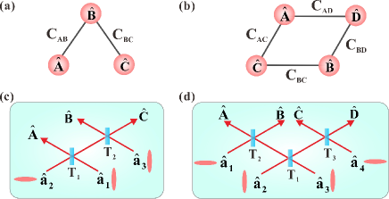
Figure 1: Schematic for achieving the weighted graph state. (a) The graph representation of a linear tripartite Gaussian weighted graph state. (b) The graph representation of a four-mode square Gaussian weighted graph state. (c) The schematic for preparing a linear tripartite Gaussian weighted graph state. (d) The schematic for preparing a four-mode square Gaussian weighted graph state.

III.2 The four-mode square weighted graph state

The graph representation of a four-mode square weighted graph state is shown in Fig. 1(b). In the ideal case, the quadrature correlations of the four-mode square Gaussian weighted graph state are expressed by

$$\hat{p}_{A}-C_{AC}\hat{x}_{C}-C_{AD}\hat{x}_{D}\rightarrow 0,$$

$$\hat{p}_{B}-C_{BC}\hat{x}_{C}-C_{BD}\hat{x}_{D}\rightarrow 0,$$

$$\hat{p}_{C}-C_{AC}\hat{x}_{A}-C_{BC}\hat{x}_{B}\rightarrow 0,$$

$$\hat{p}_{D}-C_{AD}\hat{x}_{A}-C_{BD}\hat{x}_{B}\rightarrow 0,$$ (8)

where $C_{jk\text{ }}$is the strength of interaction between modes $j$ and $k$. As shown in Fig. 1(d), the four-mode weighted graph state can be prepared by coupling two phase-squeezed and two amplitude-squeezed states of light on an optical beam-splitter network, which consists of three optical beam splitters with transmittances of $T_{1},T_{2}$ and $T_{3}$. In this paper, the four-mode weighted graph state is prepared by fixing the transmittances $T_{1}=1/5$, $T_{3}=1/2$ and adjusting the transmittance of beam splitter $T_{2}$.

Similarly, to cancel the effect of antisqueezing noise completely, the weight factors are required to satisfy $C_{AC}=C_{AD}=C_{A}=\sqrt{2T_{2}}$ and $C_{BC}=C_{BD}=C_{B}=\sqrt{2(1-T_{2})}$, respectively. Because the weight factor between mode $\hat{C}$ and neighboring modes is equal to that between mode $\hat{D}$ and neighboring modes, modes $\hat{C}$ and $\hat{D}$ are completely symmetric in the four-mode weight graph state.

In this case, the quantum correlations between the amplitude and phase quadratures of the four-mode square Gaussian weighted graph state are expressed by

$$\Delta^{2}\left(\hat{p}_{A}-C_{A}\hat{x}_{C}-C_{A}\hat{x}_{D}\right) = \left(1+4T_{2}\right)e^{-2r},$$

$$\Delta^{2}\left(\hat{p}_{B}-C_{B}\hat{x}_{C}-C_{B}\hat{x}_{D}\right) = \left(5-4T_{2}\right)e^{-2r},$$

$$\Delta^{2}\left(\hat{p}_{C}-C_{A}\hat{x}_{A}-C_{B}\hat{x}_{B}\right) = 3e^{-2r},$$

$$\Delta^{2}\left(\hat{p}_{D}-C_{A}\hat{x}_{A}-C_{B}\hat{x}_{B}\right) = 3e^{-2r},$$ (9)

where the subscripts correspond to different optical modes, $C_{A}$ and $C_{B}$ represent the weight factors, i.e., the strength of interaction between mode $\hat{A}$ and its neighboring mode ($\hat{C}$ or $\hat{D}$), and that between mode $\hat{B}$ and its neighboring mode ($\hat{C}$ or $\hat{D}$), respectively. When $T_{2}=1/2$ is chosen, the state is a four-mode square Gaussian unweighted graph state. The details of the covariance matrix for the four-mode square Gaussian weighted graph state can be found in Appendix B.

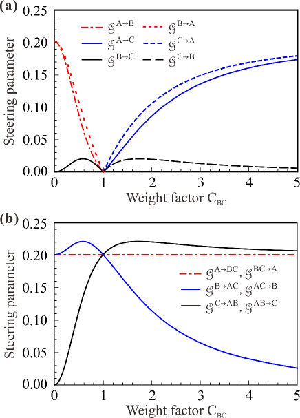
Figure 2: Dependence of steering parameter on the weight factor $C_{BC}$ in the tripartite Gaussian weighted graph state. (a) The pairwise bipartite steering between any two modes. (b) Steering parameter between one and the remaining two modes.

IV Results

IV.1 EPR steering in a linear tripartite weighted graph state

In the tripartite weighted graph state, EPR steering for (1+1) mode and (1+2) mode as a function of weight factor $C_{BC}$, as an example, under Gaussian measurement are shown in Figs. 2(a) and 2(b), respectively, where the squeezing parameter $r=0.345$ (corresponding to 3 dB squeezing) is chosen.

As shown in Fig. 2(a), EPR steering between any two modes does not exist in the condition of $C_{AB}=C_{BC}=1$, which corresponds to a linear tripartite unweighted graph state. However, EPR steering between any two modes appears in a Gaussian weighted graph state, which corresponds to the condition of $C_{BC}\neq 1$. The steerabilities $\mathcal{G}^{A\rightarrow B},\mathcal{G}^{B\rightarrow A}$ and $\mathcal{G}^{B\rightarrow C}$ are larger than zero in the condition of $C_{BC}<1$ (red lines and black solid line). The other steerabilities between two modes, including $\mathcal{G}^{A\rightarrow C},\mathcal{G}^{C\rightarrow A}$and $\mathcal{G}^{C\rightarrow B}$, exist when the weight factor is $C_{BC}>1$ (blue and black dashed lines). Especially, comparing the black solid and dashed lines in Fig. 2(a), we observe one-way EPR steering between modes $\hat{B}$ and $\hat{C}$ when the weight factor is fixed. For example, when $C_{BC}=1/2$, only $\mathcal{G}^{B\rightarrow C}$ exist. The steerability $\mathcal{G}^{A\rightarrow C}$ and $\mathcal{G}^{A\rightarrow B}$ do not exist in the case of $C_{BC}<1$ and $C_{BC}>1$, respectively. The reason for absence of the steering is the monogamy relation obtained from the two-observable EPR criterion Reid2013 : two parties cannot steer the third party simultaneously using the same steering witness. This is the same with the results of the unweighted graph state. From these results, we clearly see that EPR steering between any two modes, which does not exist in a linear tripartite CV GHZ state (an unweighted graph state) Deng2018 , exists in the tripartite Gaussian weighted graph state with nonunit weight factor.

The steering parameters between one and the other two modes in the tripartite Gaussian weighted graph state are shown in Fig. 2(b). The steerability $\mathcal{G}^{A\rightarrow BC}$ is not changed, while the steerabilities $\mathcal{G}^{B\rightarrow AC}$ and $\mathcal{G}^{C\rightarrow AB}$ are changed along with the increase of the weight factor $C_{BC}$. The reason for steerability $\mathcal{G}^{A\rightarrow BC}$ keeping unchanged with the weight factor $C_{BC}$ is that the mode $\hat{A}$ is not affected by the transmittance of beam splitter $T_{2}$; only modes $\hat{B}$ and $\hat{C}$ are related to the transmittance of beam splitter $T_{2}$.

Secret sharing is conventional protocol to distribute a secret message to a group of parties, who cannot access it individually but have to cooperate in order to decode it and prevent eavesdropping, for example, if one player (Bob) can steer the state owned by the dealer (Alice) in a three parties QSS. Bob may have the ability to decode the secret by himself, and does not need the collaboration with another player (Claire). In this case, the QSS will not be secure since one player can obtain the secret independently.

It has been shown that an unweighted tripartite Gaussian cluster state can be used as the resource of QSS since no steerabilities between any two modes exist [see the case of $C_{AB}=C_{BC}=1$ in Fig. 1(a)] Deng2018 . Here, we have to point out that the potential security risk may exist for three parties QSS using a linear tripartite Gaussian weighted graph state as a resource state, due to the existence of EPR steering between two modes. For example, when the weight factor $C_{BC}=1/2$, the steerabilities $\mathcal{G}^{A\rightarrow B},\mathcal{G}^{B\rightarrow A}$ and $\mathcal{G}^{B\rightarrow C}$ exist, which means that when any one of modes $\hat{B}$, $\hat{A}$ and $\hat{C}$ is chosen as a dealer in QSS, there will be a security risk that modes $\hat{A}$ and $\hat{B}$ may get the secret alone. The similar result can be found in the case of $C_{BC}>1$.

IV.2 EPR steering in a four-mode square weighted graph state

As shown in Fig. 1(d), based on the relation between weight factor and transmittance, we can achieve a four-mode square weighted graph state by changing the transmittance $T_{2}$. Because the weight factors have the relation of $C_{A}^{2}+C_{B}^{2}=2$, the dependence of steering parameters on the weight factor $C_{A}$ is taken as an example to analyze the steering parameters of the four-mode weighted graph state. The dependence of EPR steering on weight factor $C_{A}$ under Gaussian measurements is shown in Fig. 3, when the squeezing parameter $r=0.345$ (corresponding to 3 dB squeezing) is chosen.

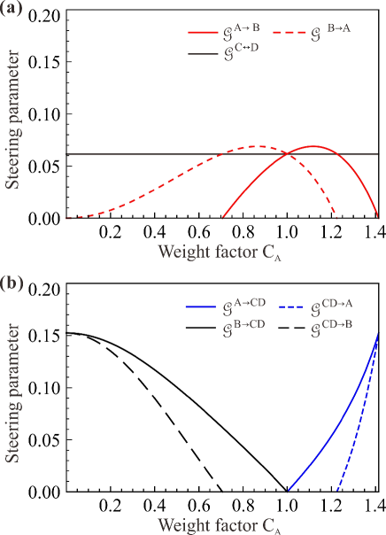
Figure 3: Difference of EPR steering between unweighted and weighted graph state, including (1+1) mode and (1+2) mode, in the four-mode square Gaussian weighted graph state. (a) Steering parameter between two diagonal modes. (b) Steering parameter between one mode ($\hat{A}$ or $\hat{B}$) and a group comprising two nearest-neighboring modes.

It has been shown that EPR steering does not exist between any two neighboring modes and between one mode and the collaboration of its two neighboring modes in a four-mode square Gaussian unweighted $\left(C_{jk}=1\right)$ cluster state Deng2017 . Different from the unweighted state, one-way EPR steering $\mathcal{G}^{A\rightarrow B}$and $\mathcal{G}^{B\rightarrow A}$ is observed in the case of $1.22<C_{A}<1.41$ and $0<C_{A}<0.71$, respectively [red solid and dashed lines in Fig. 3(a)]. EPR steering between modes $\hat{C}$ and $\hat{D}$ is invariable even if the weight factor $C_{A}$ is changed (black line). This is because the weighted graph state is obtained by changing the beam splitter $T_{2}$ between modes $\hat{A}$ and $\hat{B}$; thus the composition of modes $\hat{C}$ and $\hat{D}$ is not changed.

We also analyze the steerability between one and its two nearest modes in the four-mode square Gaussian weighted graph state, which is shown in Fig. 3(b). We can see that the EPR steering between $\hat{A}$ $(\hat{B})$ and a group comprising its two nearest-neighboring modes ($\hat{C}$ and $\hat{D}$) exists in the Gaussian weighted graph state. One-way EPR steering $\mathcal{G}^{A\rightarrow CD}$and $\mathcal{G}^{B\rightarrow CD}$ is observed in the condition of $1<C_{A}<1.22$ and $0.71<C_{A}<1$, respectively.

Here, we only present the results that steerabilities of a four-mode square Gaussian weighted graph state are different from that of a four-mode square Gaussian unweighted graph state. The details of the steerabilities of a four-mode square Gaussian unweighted graph state can be found in Ref. Deng2017 . Please note that although the optical mode is not transmitted over a lossy channel, one-way EPR steering is also presented in the Gaussian weighted graph state. The reason is that the symmetry is broken in the Gaussian weighted graph state, just as the previous observed one-way EPR steering in a lossy channel Deng2017 .

IV.3 Verification of CKW-type monogamy relation

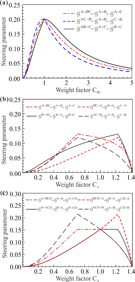
Figure 4: Monogamy relation in the Gaussian weighted graph state. (a) The monogamy relation for all types EPR steering between one and the other two modes in the tripartite Gaussian weighted graph state. (b),(c) Validation of generalized CKW-type monogamy for steering in the four-mode square Gaussian weighted graph state.

The Coffman-Kundu-Wootters(CKW)-type monogamy relations Coffman2000 , which quantify how the steering is distributed among different subsystems Xiang2017 , are expressed by

$$\mathcal{G}^{k\rightarrow(i,j)}(\sigma_{ijk})-\mathcal{G}^{k\rightarrow i}(\sigma_{ijk})-\mathcal{G}^{k\rightarrow j}(\sigma_{ijk}) \geq 0,$$

$$\mathcal{G}^{(i,j)\rightarrow k}(\sigma_{ijk})-\mathcal{G}^{i\rightarrow k}(\sigma_{ijk})-\mathcal{G}^{j\rightarrow k}(\sigma_{ijk}) \geq 0,$$ (10)

where $i,j,k\in\{\hat{A},\hat{B},\hat{C}\}$ in the tripartite weighted graph state. Here, we confirm the CKW-type monogamy relation is coincident for all types of EPR steering in the linear tripartite and four-mode square Gaussian weighted graph state, as shown in Fig. 4.

Figure. 4(a) shows the CKW-type monogamy relation in the tripartite Gaussian weighted graph state. When the weight factor $C_{BC}<1$, the CKW-type monogamy relations $\mathcal{G}^{A\rightarrow BC}-\mathcal{G}^{A\rightarrow B}-\mathcal{G}^{A\rightarrow C}=$ $\mathcal{G}^{C\rightarrow AB}-\mathcal{G}^{C\rightarrow A}-\mathcal{G}^{C\rightarrow B}$ (red dashed-dotted line), $\mathcal{G}^{B\rightarrow AC}-\mathcal{G}^{B\rightarrow A}-\mathcal{G}^{B\rightarrow C}=\mathcal{G}^{BC\rightarrow A}-\mathcal{G}^{B\rightarrow A}-\mathcal{G}^{C\rightarrow A}=$ $\mathcal{G}^{AB\rightarrow C}-\mathcal{G}^{A\rightarrow C}-\mathcal{G}^{B\rightarrow C}$ (black solid line), and $\mathcal{G}^{AC\rightarrow B}-\mathcal{G}^{A\rightarrow B}-\mathcal{G}^{C\rightarrow B}$ (blue dashed line) are valid, respectively. When the weight factor $C_{BC}>1,$ the CKW-type monogamy relations $\mathcal{G}^{A\rightarrow BC}-\mathcal{G}^{A\rightarrow B}-\mathcal{G}^{A\rightarrow C}=$ $\mathcal{G}^{B\rightarrow AC}-\mathcal{G}^{B\rightarrow A}-\mathcal{G}^{B\rightarrow C}$ (red dashed-dotted line), $\mathcal{G}^{C\rightarrow AB}-\mathcal{G}^{C\rightarrow A}-\mathcal{G}^{C\rightarrow B}=\mathcal{G}^{BC\rightarrow A}-\mathcal{G}^{B\rightarrow A}-\mathcal{G}^{C\rightarrow A}=$ $\mathcal{G}^{AC\rightarrow B}-\mathcal{G}^{A\rightarrow B}-\mathcal{G}^{C\rightarrow B}$ (blue dashed line), and $\mathcal{G}^{AB\rightarrow C}-\mathcal{G}^{A\rightarrow C}-\mathcal{G}^{B\rightarrow C}$ (black solid line) are also valid, respectively.

We also confirm the general monogamy relations in the four-mode square Gaussian weighted graph state genemono , especially the steerabilities that are different from that of the unweighted graph state, are valid, as shown in Figs. 4(b)-4(c), where $i,j,k\in\{\hat{A},\hat{B},\hat{C},\hat{D}\}$ or $\{\hat{A},\hat{C}\hat{D},\hat{B}\}$. The CKW-type monogamy relations, including EPR steering between modes $\hat{A}\$and $\hat{B}$, are shown in Fig. 4(b). Due to the symmetry of modes $\hat{C}\$ and $\hat{D}$, the validation of monogamy relations for mode $\hat{C}\$ are suitable for $\hat{D}$. The generalized CKW-type monogamy relations are also valid, as shown in Fig. 4(c).

When $i,j,k\in\{\hat{A},\hat{C},\hat{D}\}$ are chosen, the steerabilities $\mathcal{G}^{A\rightarrow CD}$ and $\mathcal{G}^{CD\rightarrow A}$ exist for the four-mode square Gaussian weighted graph state as shown in Fig. 3(b). The EPR steering between modes $\hat{A}\$ and $\hat{C}(\hat{D})$ for the four-mode square weighted graph state does not exist, i.e., $\mathcal{G}^{A\rightarrow C}=0$ and $\mathcal{G}^{C\rightarrow A}=0$, which is the same as that of the four-mode square unweighted graph state as shown in Ref. Deng2017 . The CKW-type monogamy relations $\mathcal{G}^{A\rightarrow CD}-\mathcal{G}^{A\rightarrow C}-\mathcal{G}^{A\rightarrow D}\geq 0$ and $\mathcal{G}^{CD\rightarrow A}-\mathcal{G}^{C\rightarrow A}-\mathcal{G}^{D\rightarrow A}\geq 0$ are always valid. The same results are obtained for steerabilities among mode $\hat{B}$ and modes ($\hat{C}$, $\hat{D}$).

V Discussion and conclusion

EPR steering analyzed in this paper are arbitrary bipartite separations of a tripartite and four-mode Gaussian weighted graph states based on the necessary and sufficient criterion under Gaussian measurements Kogias2015 , which quantifies EPR steering for bipartite separations of a multipartite Gaussian state. A quantum system involving more than three subsystems has different possible partitions, and it has been discussed for entanglement Multient1 ; Multient2 ; Multient3 and Bell nonlocality MultiBell1 ; MultiBell2 . For EPR steering of Gaussian states, the criterion which is used to quantify the quantum steering for multipartition of a multipartite Gaussian state remains an open question until now and it is worthy of further investigation.

The study on quantum nonlocality and EPR steering has deepened our understanding of the foundation of quantum theory. Recently, postquantum nonlocality has been discussed in discrete Post1 and continuous variable scenarios Post2 ; Post3 . The postquantum steering has been studied in a discrete scenario Post4 ; Post5 . However, the postquantum steering for a continuous variable system has not been discussed, which remains an open question.

In this paper, the quantum states are Gaussian states of a continuous variable system and the measurements are Gaussian measurements. The necessary and sufficient criterion for EPR steering of a Gaussian state proposed in Ref. Kogias2015 is used to quantify the EPR steering in Gaussian weighted graph states.Recently, it has been shown that non-Gaussian measurements can lead to extra steerability even for Gaussian states OneWayPryde ; nonGaussian2 , and might allow for circumventing some monogamy constraints Reid2013 ; nonGaussian3 ; nonGaussian4 . It will be interesting to investigate EPR steering in Gaussian weighted graph states with non-Gaussian measurements.

In conclusion, steering parameters in a linear tripartite and a four-mode square Gaussian weighted graph state are presented. Comparing with the unweighted graph state, we conclude that a weighted graph state features richer steering properties. EPR steering that is absent in the Gaussian unweighted graph state is presented in the Gaussian weighted graph state. The pairwise bipartite steering exists in the tripartite Gaussian weighted graph state. EPR steering between one and its two nearest modes is also observed in the four-mode square Gaussian weighted graph state, which could not be obtained in the four-mode square Gaussian unweighted graph state. We also show that the CKW-type monogamy relations are valid in the Gaussian weighted graph states.

We also analyze quantum entanglement in the linear tripartite and four-mode square Gaussian weighted graph state. Different from the quantum steering, quantum entanglement is always maintained in the linear tripartite and four-mode square Gaussian weighted graph state. This result is the same as that obtained in Ref. JZhang2010 , where the entanglement of the weighted graph state is analyzed.

QSS can be implemented when the players are separated in a local quantum network and collaborate to decode the secret sent by the dealer who owns the other one mode GHZQSS1 . In this case, the dealer must not be steered by any one of two players; only the collective steerability is needed. Thus the presence of EPR steering between any two modes in a linear tripartite Gaussian weighted graph state shows that the Gaussian weighted graph state is not a good resource for QSS.

There are other suitable quantum information tasks using EPR steering in a Gaussian weighted graph state as a resource. For example, for the tripartite Gaussian weighted graph state with weight factor $0<C_{BC}<1$, the steerability between modes $\hat{A}$ and $\hat{B}$ always exists, and only the steerability from $\hat{B}$ to $\hat{C}$ exists. In this case, the state can be used as resource state of quantum conference Conference1 ; Conference2 . Especially, the user B (who owns mode $\hat{B}$) can send information to users A (who owns mode $\hat{A}$) and C (who owns mode $\hat{C}$), and the communication between users B and C is one-way since only steerability from modes $\hat{B}$ to $\hat{C}$ exists. Thus this kind of quantum conference based on the tripartite Gaussian weighted graph state is one-way quantum conference, in which only user B can send information to users A and C, while users A and C can not send information to user B.

APPENDIX

V.1 Preparation scheme of the linear tripartite Gaussian weighted graph state

In this appendix, we present details of the preparation scheme for the tripartite Gaussian weighted graph state. As shown in Fig. 1(c) in the main text, the tripartite Gaussian weighted graph state is prepared by coupling three squeezed states on two optical beam splitters $T_{1}$ and $T_{2}$. Three input squeezed states are expressed by

$$\hat{a}_{1} =e^{-r_{1}}\hat{x}_{1}^{(0)}+ie^{r_{1}}\hat{p}_{1}^{(0)},$$

$$\hat{a}_{2} =e^{r_{2}}\hat{x}_{2}^{(0)}+ie^{-r_{2}}\hat{p}_{2}^{(0)},$$

$$\hat{a}_{3} =e^{-r_{3}}\hat{x}_{3}^{(0)}+ie^{r_{3}}\hat{p}_{3}^{\left(0\right)},$$ (A1)

where $r_{i}$ ($i=1,2,3$) is the squeezing parameter, and the superscript of the amplitude and phase quadratures represent the vacuum state. Under this notation, the variances of amplitude and phase quadratures for vacuum state are $\Delta^{2}\hat{x}^{(0)}=\Delta^{2}\hat{p}^{(0)}=1$. The transformation matrix of the beam-splitter network is

$$U_{1}=\left[\begin{array}[]{ccc}-\sqrt{T_{1}}&-\sqrt{1-T_{1}}&0\\ i\sqrt{(1-T_{1})(1-T_{2})}&-i\sqrt{T_{1}(1-T_{2})}&\sqrt{T_{2}}\\ -\sqrt{(1-T_{1})T_{2}}&\sqrt{T_{1}T_{2}}&-i\sqrt{1-T_{2}}\end{array}\right],$$ (A2)

After the conversion of the beam-splitter network, the output modes are given by

$$\hat{A} =-\sqrt{T_{1}}\hat{a}_{1}-\sqrt{1-T_{1}}\hat{a}_{2},$$

$$\hat{B} =i\sqrt{(1-T_{1})(1-T_{2})}\hat{a}_{1}-i\sqrt{T_{1}(1-T_{2})}\hat{a}_{2}+\sqrt{T_{2}}\hat{a}_{3},$$

$$\hat{C} =-\sqrt{(1-T_{1})T_{2}}\hat{a}_{1}+\sqrt{T_{1}T_{2}}\hat{a}_{2}-i\sqrt{1-T_{2}}\hat{a}_{3},$$ (A3)

respectively. Here, we assume that the squeezed parameters of all the squeezed states are equal $(r_{1}=r_{2}=r_{3}=r)$.

The Gaussian state can be completely characterized by a covariance matrix. Based on the expressions of input and output states, the covariance matrix of the tripartite Gaussian weighted graph state is expressed by

$$\sigma_{ABC}=\left[\begin{array}[]{ccc}\sigma_{A}&f\mathbf{\Omega}&g\mathbf{Z}\\ f\mathbf{\Omega}&\sigma_{B}&h\mathbf{\Omega}\\ g\mathbf{Z}&h\mathbf{\Omega}&\sigma_{C}\end{array}\right],$$ (A4)

where                

$\ \ \ \ \ \ \ \ \ \ \ \ \ \ \ f=\frac{\sqrt{2(1-T_{2})}(e^{2r}-e^{-2r})}{3},$

$\ \ \ \ \ \ \ \ \ \ \ \ \ \ \ g=\frac{\sqrt{2T_{2}}(e^{-2r}-e^{2r})}{3},\ \ \ \ \ \ \ \ \ \ \ \ \ \ \ \$

$\ \ \ \ \ \ \ \ \ \ \ \ \ \ \ h=\frac{2\sqrt{T_{2}(1-T_{2})}(e^{2r}-e^{-2r})}{3},$

$\ \ \ \ \ \ \mathbf{\Omega=}\begin{pmatrix}0&1\\ 1&0\end{pmatrix},\qquad\mathbf{Z}=\begin{pmatrix}1&0\\ 0&-1\end{pmatrix},$

$\ \ \ \sigma_{A}=\left(\begin{array}[]{cc}\frac{1}{3}e^{-2r}+\frac{2}{3}e^{2r}&0\\ 0&\frac{2}{3}e^{-2r}+\frac{1}{3}e^{2r}\end{array}\right),$

$\sigma_{B}=\left(\begin{array}[]{cc}\frac{2(1-T_{2})e^{2r}+(1+2T_{2})e^{-2r}}{3}&0\\ 0&\frac{2(1-T_{2})e^{-2r}+(1+2T_{2})e^{2r}}{3}\end{array}\right),$

$\sigma_{C}=\left(\begin{array}[]{cc}\frac{3-2T_{2}}{3}e^{2r}+\frac{2T_{2}}{3}e^{-2r}&0\\ 0&\frac{3-2T_{2}}{3}e^{-2r}+\frac{2T_{2}}{3}e^{2r}\end{array}\right),$ respectively.          

V.2 Preparation scheme of the four-mode square Gaussian weighted graph state

As shown in Fig. 1(d) in the main text, the four-mode square Gaussian weighted graph state is prepared by coupling four squeezed states on an optical beam-splitter network. Four input squeezed states are expressed by

$$\hat{a}_{1} =e^{r_{1}}\hat{x}_{1}^{(0)}+ie^{-r_{1}}\hat{p}_{1}^{(0)},$$

$$\hat{a}_{2} =e^{-r_{2}}\hat{x}_{2}^{(0)}+ie^{r_{2}}\hat{p}_{2}^{(0)},$$

$$\hat{a}_{3} =e^{-r_{3}}\hat{x}_{3}^{(0)}+ie^{r_{3}}\hat{p}_{3}^{\left(0\right)},$$

$$\hat{a}_{4} =e^{r_{4}}\hat{x}_{4}^{(0)}+ie^{-r_{4}}\hat{p}_{4}^{\left(0\right)},$$ (A5)

When the transmittances of $T_{1}=1/5$ and $T_{3}=1/2$ are chosen, the transformation matrix of the beam-splitter network is given by

$$U_{2}=\left[\begin{array}[]{cccc}-\sqrt{1-T_{2}}&-2\sqrt{\frac{T_{2}}{5}}&-i\sqrt{\frac{T_{2}}{5}}&0\\ \sqrt{T_{2}}&-2\sqrt{\frac{1-T_{2}}{5}}&-i\sqrt{\frac{1-T_{2}}{5}}&0\\ 0&\frac{i}{\sqrt{10}}&\sqrt{\frac{2}{5}}&-\frac{1}{\sqrt{2}}\\ 0&\frac{i}{\sqrt{10}}&\sqrt{\frac{2}{5}}&\frac{1}{\sqrt{2}}\end{array}\right],$$ (A6)

Thus the output modes from the optical beam-splitter network are expressed by

$$\hat{A} =-\sqrt{1-T_{2}}\hat{a}_{1}-2\sqrt{\frac{T_{2}}{5}}\hat{a}_{2}-i\sqrt{\frac{T_{2}}{5}}\hat{a}_{3},$$

$$\hat{B} =\sqrt{T_{2}}\hat{a}_{1}-2\sqrt{\frac{1-T_{2}}{5}}\hat{a}_{2}-i\sqrt{\frac{1-T_{2}}{5}}\hat{a}_{3},$$

$$\hat{C} =\frac{i}{\sqrt{10}}\hat{a}_{2}+\sqrt{\frac{2}{5}}\hat{a}_{3}-\frac{1}{\sqrt{2}}\hat{a}_{4},$$

$$\hat{D} =\frac{i}{\sqrt{10}}\hat{a}_{2}+\sqrt{\frac{2}{5}}\hat{a}_{3}+\frac{1}{\sqrt{2}}\hat{a}_{4},$$ (A7)

respectively. Here, we assume that the squeezed parameters of all the squeezed states are equal $(r_{1}=r_{2}=r_{3}=r_{4}=r)$.

According to the information of input and output states, the covariance matrix of the four-mode square Gaussian weighted graph state is expressed by

$$\sigma_{ABCD}=\left[\begin{array}[]{cccc}\sigma_{A}&l\mathbf{Z}&m\mathbf{\Omega}&s\mathbf{\Omega}\\ l\mathbf{Z}&\sigma_{B}&n\mathbf{\Omega}&v\mathbf{\Omega}\\ m\mathbf{\Omega}&n\mathbf{\Omega}&\sigma_{C}&w\mathbf{Z}\\ s\mathbf{\Omega}&v\mathbf{\Omega}&w\mathbf{Z}&\sigma_{D}\end{array}\right].$$ (A8)

where

$\ \ \ \ \ \ \ \ \ \ \ \ l=\frac{4\sqrt{T_{2}(1-T_{2})}(e^{-2r}-e^{2r})}{5},$

$\ \ \ \ \ \ \ \ \ \ \ m=\frac{\sqrt{2T_{2}}(e^{2r}-e^{-2r})}{5},$

$\ \ \ \ \ \ \ \ \ \ \ \ n=\frac{\sqrt{2(1-T_{2})}(e^{2r}-e^{-2r})}{5},$

$\ \ \ \ \ \ \ \ \ \ \ \ s=\frac{\sqrt{2T_{2}}(e^{2r}-e^{-2r})}{5},$

$\ \ \ \ \ \ \ \ \ \ \ v=\frac{\sqrt{2(1-T_{2})}(e^{2r}-e^{-2r})}{5},$

$\ \ \ \ \ \ \ \ \ \ \ \ w=\frac{2(e^{-2r}-e^{2r})}{5},$

$\sigma_{A}=\left(\begin{array}[]{cc}\frac{5-4T_{2}}{5}e^{2r}+\frac{4T_{2}}{5}e^{-2r}&0\\ 0&\frac{5-4T_{2}}{5}e^{-2r}+\frac{4T_{2}}{5}e^{2r}\end{array}\right),$

$\sigma_{B}=\left(\begin{array}[]{cc}\frac{(1+4T_{2})e^{2r}+4(1-T_{2})e^{-2r}}{5}&0\\ 0&\frac{(1+4T_{2})e^{-2r}+4(1-T_{2})e^{2r}}{5}\end{array}\right),$

$\sigma_{C}=\left(\begin{array}[]{cc}\frac{3}{5}e^{2r}+\frac{2}{5}e^{-2r}&0\\ 0&\frac{3}{5}e^{-2r}+\frac{2}{5}e^{2r}\end{array}\right),$

$\sigma_{D}=\left(\begin{array}[]{cc}\frac{3}{5}e^{2r}+\frac{2}{5}e^{-2r}&0\\ 0&\frac{3}{5}e^{-2r}+\frac{2}{5}e^{2r}\end{array}\right),$

respectively.

Based on the covariance matrices of the linear tripartite and the four-mode square Gaussian weighted graph states, the property of the weighted graph states can be verified.

References

- (1) A. Einstein, B. Podolsky, and N. Rosen, Phys. Rev. 47, 777 (1935).
- (2) E. Schrödinger, Proc. Cambridge Philos. Soc. 31, 555 (1935).
- (3) E. Schrödinger, Proc. Cambridge Philos. Soc. 32, 446 (1936).
- (4) D. J. Saunders, S. J. Jones, H. M. Wiseman, and G. J. Pryde, Nat. Phys. 6, 845 (2010).
- (5) J. S. Bell, Physics 1, 195 (1964).
- (6) R. Horodecki, P. Horodecki, M. Horodecki, and K. Horodecki, Rev. Mod. Phys. 81, 865 (2009).
- (7) S. J. Jones, H. M. Wiseman, and A. C. Doherty, Phys. Rev. A 76, 052116 (2007).
- (8) P. Skrzypczyk, M. Navascués, and D. Cavalcanti, Phys. Rev. Lett. 112, 180404 (2014).
- (9) H. M. Wiseman, S. J. Jones, and A. C. Doherty, Phys. Rev. Lett. 98, 140402 (2007).
- (10) V. Händchen, T. Eberle, S. Steinlechner, A. Samblowski, T. Franz, R. F. Werner, and R. Schnabel, Nat. Photon. 6, 596 (2012).
- (11) S. Armstrong, M. Wang, R. Y. Teh, Q. Gong, Q. He, J. Janousek, H. A. Bachor, M. D. Reid, and P. K. Lam, Nat. Phys. 11, 167 (2015).
- (12) S. Wollmann, N. Walk, A. J. Bennet, H. M. Wiseman, and G. J. Pryde, Phys. Rev. Lett. 116, 160403 (2016).
- (13) K. Sun, X.-J. Ye, J.-S. Xu, X.-Y. Xu, J.-S. Tang, Y.-C. Wu, J.-L. Chen, C.-F.Li, and G.-C. Guo, Phys. Rev. Lett. 116, 160404 (2016).
- (14) C. Branciard, E. G. Cavalcanti, S. P. Walborn, V. Scarani, and H. M. Wiseman, Phys. Rev. A 85, 010301 (2012).
- (15) M. Piani and J. Watrous, Phys. Rev. Lett. 114, 060404 (2015).
- (16) M. D. Reid, Phys. Rev. A 88, 062338 (2013).
- (17) Q. He, L. Rosales-Zárate, G. Adesso, and M. D. Reid, Phys. Rev. Lett. 115, 180502 (2015).
- (18) Y. Xiang, I. Kogias, G. Adesso, and Q. He, Phys. Rev. A 95, 010101(R) (2017).
- (19) M. Wang, Z. Qin, and X. Su, Phys. Rev. A 95, 052311 (2017).
- (20) M. Wang, Z. Qin, Y. Wang, and X. Su, Phys. Rev. A 96, 022307 (2017).
- (21) Z. Qin, X. Deng, C. Tian, M. Wang, X. Su, C. Xie, and K. Peng, Phys. Rev. A 95, 052114 (2017).
- (22) D. Cavalcanti, P. Skrzypczyk, G. H. Aguilar, R. V. Nery, P. H. Souto Ribeiro, and S. P. Walborn, Nat. Commun. 6, 7941 (2015).
- (23) C. M. Li, K. Chen, Y. N. Chen, Q. Zhang, Y. A. Chen, and J. W. Pan, Phys. Rev. Lett. 115, 010402 (2015).
- (24) X. Deng, Y. Xiang, C. Tian, G. Adesso, Q. He, Q. Gong, X. Su, C. Xie, and K. Peng, Phys. Rev. Lett. 118, 230501 (2017).
- (25) H. J. Briegel and R. Raussendorf, Phys. Rev. Lett. 86, 910 (2001).
- (26) J. Zhang and S. L. Braunstein, Phys. Rev. A 73, 032318 (2006).
- (27) M. Hein, J. Eisert, and H. J. Briegel, Phys. Rev. A 69, 062311 (2004).
- (28) N. C. Menicucci, S. T. Flammia, and P. van Loock, Phys. Rev. A 83, 042335 (2011).
- (29) J. Zhang, Phys. Rev. A 82, 034303 (2010).
- (30) P. Xue, Phys. Rev. A 86, 023812 (2012).
- (31) I. Kogias, Y. Xiang, Q. He, and G. Adesso, Phys. Rev. A 95, 012315 (2017).
- (32) M. Wang, Y. Xiang, Q. He, and Q. Gong, Phys. Rev. A 91, 012112 (2015).
- (33) P. van Loock and S. L. Braunstein, Phys. Rev. Lett. 84, 3482 (2000).
- (34) H. Yonezawa, T. Aoki, and A. Furusawa, Nature 431, 430 (2004).
- (35) J. Jing, J. Zhang, Y. Yan, F. Zhao, C. Xie, and K. Peng, Phys. Rev. Lett. 90, 167903 (2003).
- (36) R. Raussendorf and H. J. Briegel, Phys. Rev. Lett. 86, 5188 (2001).
- (37) X. Su, S. Hao, X. Deng, L. Ma, M. Wang, X. Jia, C. Xie, and K. Peng, Nat. Commun. 4, 2828 (2013).
- (38) M. D. Reid, Phys. Rev. A 88, 062108 (2013).
- (39) V. Coffman, J. Kundu, and W. K. Wootters, Phys. Rev. A 61, 052306 (2000).
- (40) I. Kogias, A. R. Lee, S. Ragy, and G. Adesso, Phys. Rev. Lett. 114, 060403 (2015).
- (41) X. Deng, C. Tian, M. Wang, Z. Qin, and X. Su, Opt. Commun. 421, 14 (2018).
- (42) L. Lami, C. Hirche, G. Adesso, and A. Winter, Phys. Rev. Lett. 117, 220502 (2016).
- (43) J. Sperling and W. Vogel, Phys. Rev. Lett. 111, 110503 (2013).
- (44) S. Gerke, J. Sperling, W. Vogel, Y. Cai, J. Roslund, N. Treps, and C. Fabre, Phys. Rev. Lett. 114, 050501 (2015).
- (45) Z. Qin, M. Gessner, Z. Ren, X. Deng, D. Han, W. Li, X. Su, A. Smerzi and K. Peng, npj Quantum Inf. 5, 3 (2019).
- (46) S. Sami and I. Chakrabarty, and A. Chaturvedi, Phys. Rev. A 96, 022121 (2017).
- (47) M. C. Tran, R. Ramanathan, M. McKague, D. Kaszlikowski, and T. Paterek, Phys. Rev. A 98, 052325 (2018).
- (48) S. Popescu t and D. Rohrlich, Found.Phys. 24, 379 (1994).
- (49) A. Ketterer, A. Laversanne-Finot, and L. Aolita, Phys. Rev. A 97, 012133 (2018).
- (50) P. Cherian J, A. Mukherjee, A. Roy, S. S. Bhattacharya, and M. Banik, Phys. Rev. A 99, 012105 (2019).
- (51) A. B. Sainz, N. Brunner, D. Cavalcanti, P. Skrzypczyk, and T. Vértesi, Phys. Rev. Lett. 115, 190403 (2015).
- (52) M. Banik, J. Math. Phys. 56, 052101 (2015).
- (53) S. -W. Ji, J. Lee, J. Park, and H. Nha, Sci. Rep. 6, 29729 (2016).
- (54) S. -W. Ji, M. S. Kim, and H. Nha, J. Phys. A: Math. Theor. 48, 135301 (2015).
- (55) G. Adesso and R. Simon, J. Phys. A: Math. Theor. 49, 34LT02 (2016).
- (56) Y. Wu, J. Zhou, X. Gong, Y. Guo, Z.-M. Zhang, and G. He, Phys. Rev. A 93, 022325 (2016).
- (57) Y. Wang, C. Tian, Q. Su, M. Wang, X. Su, Sci. Chin. Inf. Sci. 62, 072501 (2019).