The breaking of continuous scale invariance to discrete scale invariance: a universal quantum phase transition

Abstract

We provide a review on the physics associated with phase transitions in which continuous scale invariance is broken into discrete scale invariance. The rich features of this transition characterized by the abrupt formation of a geometric ladder of eigenstates, low energy universality without fixed points, scale anomalies and Berezinskii-Kosterlitz-Thouless scaling is described. The important role of this transition in various celebrated single and many body quantum systems is discussed along with recent experimental realizations. Particular focus is devoted to a recent realization in graphene.

1 Introduction

Continuous scale invariance (CSI) – a common property of physical systems – describes the invariance of a physical quantity $f(x)$ (e.g., the mass) when changing a control parameter $x$ (e.g., the length). This property is expressed by a simple scaling relation,

$$f(ax)=b\,f(x),$$ (1.1)

satisfied $\forall a>0$ and corresponding $b(a)$, whose general solution is the power law

$$f(x)=C\,x^{\gamma}$$ (1.2)

with $\gamma=\ln b/\ln a$. Other physical systems possess the weaker discrete scale invariance (DSI) expressed by the same scaling relation (1.1) but now satisfied for fixed values $a,b$ and whose solution becomes

$$f(x)=x^{\gamma}\,G\left(\ln x/\ln a\right),$$ (1.3)

where $G(u+1)=G(u)$. Since $G\left(u\right)$ is a periodic function, one can expand it in Fourier series $G\left(u\right)=\sum c_{n}e^{2\pi inu}$, thus,

$$f\left(x\right)=\sum_{n=-\infty}^{\infty}c_{n}x^{\gamma+i\frac{2\pi n}{\ln a}}.$$ (1.4)

If $f\left(x\right)$ is required to obey CSI, $G\left(u\right)$ would be constraint to fulfill the relation $G\left(u\right)=G\left(u+a_{0}\right)\>\forall a_{0}\in\mathbb{R}$. In this case, $G\left(u\right)$ can only be a constant function, that is, $c_{n}=0$ for all $n\neq 0$ eliminating all terms with complex exponents in (1.4). Therefore, real exponents are a signature of CSI and complex exponents are a signature of DSI.

In this article we describe a variety of distinct quantum systems in which a sharp transition initiates the breaking of CSI into DSI. Essential to all these cases is a DSI phase characterized by a sudden appearance of a low energy spectrum arranged in an infinite geometric series. Accordingly, each transition is associated with exponents that change from real to complex valued at the critical point. We describe the universal properties of this transition. Particularly, in the framework of the renormalization group it is shown that universality in this case is not associated with trajectories terminating at a fixed point but with periodic flow known as a limit cycle. Intrinsic to this phenomena is a special type of scale anomaly in which residual discrete scaling symmetry remains at the quantum level.

We discuss the physical realizations of the CSI to DSI transition and present recent experimental observations which provide evidence for the existence of the critical point and for the universal low energy features of the DSI phase. We discuss the basic ingredients that underline these features and the possibility of their occurrence in other, yet to be studied systems.

2 The Schrödinger $1/r^{2}$ potential

A well studied example exhibiting the breaking of CSI to DSI is given by the problem of a quantum particle in an attractive inverse square potential [1, 2] described by the Hamiltonian ($\hbar=1,\,m=1/2$)

$$H_{S}=p^{2}-\lambda/r^{2}.$$ (2.1)

This system constitutes an effective description of the “Efimov effect” [3, 4] and plays a role in various other systems [5, 6, 7, 8, 9].

2.1 The spectral properties of $H_{S}$

The Hamiltonian $H_{S}$ has an interesting yet disturbing property – the power law form of the potential matches the order of the kinetic term. As a result, the Schrödinger equation

$$H_{S}\psi=E\psi$$ (2.2)

depends on the single dimensionless parameter $\lambda$ which raises the question of the existence of a characteristic energy to express the eigenvalues $E_{n}$. This absence of characteristic scale implies the invariance of $H_{S}\psi=E\psi$ under the scale transformation [10]

$$x^{i}\rightarrow ax^{i},\,E\rightarrow a^{-2}E$$ (2.3)

which indicates that if there is one negative energy bound state $E_{n}$ then there is an unbounded continuum of bound states which render the Hamiltonian nonphysical and mathematically not self-adjoint [11, 12].

The eigenstates of $H_{S}$ can be solved in terms of Bessel functions which confirm these assertions in more detail. For $E<0$ and lowest orbital angular momentum subspace $l=0$, the most general decaying solution is described by the radial function

$$\psi\left(r\right)\approx r^{-\frac{d-2}{2}}\left(\left(kr\right)^{-\sqrt{\lambda_{c}-\lambda}}\left(a_{1}+\mathcal{O}\left(kr\right)^{2}\right)+\left(kr\right)^{\sqrt{\lambda_{c}-\lambda}}\left(a_{2}+\mathcal{O}\left(kr\right)^{2}\right)\right)$$ (2.4)

where $k\equiv\sqrt{-E}$, $a_{1},\,a_{2}$ are energy independent coefficients, $d$ is the space dimension and $\lambda_{c}\equiv(d-2)^{2}/4$ . As seen in (2.4), for $\lambda>\lambda_{c}-1$, $\psi_{0}\left(r\right)$ is normalizable $\forall\,\mathrm{Re}\,\left(E\right)<0$ which constitutes a continuum of complex valued bound states of $H_{S}$. Thus, for $\lambda>\lambda_{c}-1$, $H_{S}$ is no longer self-adjoint, a property that originates from the strong singularity of the potential and is characteristic of a general class of potentials with high order of singularity [1].

A simple, physically instructive procedure to deal with the absence of self-adjointness is to remove the singular $r=0$ point by introducing a short distance cutoff $L$ and to apply a boundary condition at $r=L$ [9, 13, 14, 15, 16, 17, 18]. The most general boundary condition is the mixed condition

$$L\frac{\psi^{\prime}\left(L\right)}{\psi\left(L\right)}=g,$$ (2.5)

$g\in\mathbb{R}$, for which there is an infinite number of choices each describing different short range physics.

Equipped with condition (2.5) the operator $H_{S}$ is now a well defined self-adjoint operator on the interval $L<r<\infty$. The spectrum of $H_{S}$ exhibits two distinct features in the low energy $kL\ll 1$ regime. For $\lambda<\lambda_{c}\equiv\left(d-2\right)^{2}/4$, the expression of $L\psi^{\prime}\left(L\right)/\psi\left(L\right)$ as given from (2.4) is independent of $k$ to leading order in $kr$. As a result, equation (2.5) does not hold for a general choice of $g$. For $\lambda>\lambda_{c}$, the insertion of (2.4) into (2.5) leads to

$$\left(kL\right)^{2i\sqrt{\lambda-\lambda_{c}}}=e^{i\gamma}$$ (2.6)

where $\gamma\left(g,\lambda\right)$ is a phase that can be calculated (the explicit expression of $\gamma$ is not important for the purpose of this section). The solution of (2.6) yields a set of bound states with energies

$$k_{n}=k_{0}e^{-\frac{\pi n}{\sqrt{\lambda-\lambda_{c}}}}$$ (2.7)

where $n\in Z$, such that $k_{n}L\ll 1$ and $k_{0}\equiv\frac{1}{L}e^{\frac{\gamma}{2\sqrt{\lambda-\lambda_{c}}}}$. Thus, for $\lambda<\lambda_{c}\equiv\left(d-2\right)^{2}/4$, the spectrum contains no bound states close to $E=0$, however, as $\lambda$ goes above $\lambda_{c}$, an infinite series of bound states appears. Moreover, in this ”over-critical” regime, the states arrange in a geometric series such that

$$k_{n+1}/k_{n}=e^{-\frac{\pi}{\sqrt{\lambda-\lambda_{c}}}}.$$ (2.8)

The absence of any states for $\lambda<\lambda_{c}$ is a signature of CSI while the geometric structure of (2.7) for $\lambda>\lambda_{c}$ is a signature of DSI since $k_{n}$ is invariant under $\left\{k_{n}\right\}\to\left\{\exp\left(-\pi/\sqrt{\lambda-\lambda_{c}}\right)k_{n}\right\}$. Accordingly, as seen in (2.4), the characteristic behavior of the eigenstates for $kr\ll 1$ manifests an abrupt transition from real to complex valued exponents as $\lambda$ exceeds $\lambda_{c}$. Thus, $H_{S}$ exhibits a quantum phase transition (QPT) at $\lambda_{c}$ between a CSI phase and a DSI phase. The characteristics of this transition are independent of the values of $L,g$ which enter only into the overall factor $k_{0}$ in (2.7). The functional dependence of $k_{n}$ on $\sqrt{\lambda-\lambda_{c}}$ is characteristic of Berezinskii-Kosterlitz-Thouless (BKT) transitions as was identified in [7, 19, 20, 21]. Finally, the breaking of CSI to DSI in the $\lambda>\lambda_{c}$ regime constitutes a special type of scale anomaly since a residual symmetry remains even after regularization (see Table 1).

Table 1: Summary of the properties associated with the transition occurring at $\lambda=\lambda_{c}$ for the Hamiltonian $H_{S}$ given in equation (2.1) on the interval $L<r<\infty$.

	$\lambda<\lambda_{c}$	$\lambda>\lambda_{c}-1$	$\lambda>\lambda_{c}$	Scale anomaly $\implies$
Formal Hamiltonian	CSI	CSI	CSI
Self-adjointness	$H=H^{\dagger}$	$H\neq H^{\dagger}$	$H\neq H^{\dagger}$
Regularization with $L$	Redundant	Essential	Essential
Symmetry of eigenspace	CSI	CSI	DSI
Quantum Phase Transition $\implies$

2.2 Physical realizations of $H_{S}$

A well known realization of $H_{S}$ for $\lambda>\lambda_{c}$ is the “Efimov effect” [3, 4, 22]. In $1970$, Efimov studied the quantum problem of three identical nucleons of mass $m$ interacting through a short range ($r_{0}$) potential. He pointed out that when the scattering length $a$ of the two-body interaction becomes very large, $a\gg r_{0}$, there exists a scale-free regime for the low-energy spectrum, $\hbar^{2}/ma^{2}\ll E\ll\hbar^{2}/mr_{0}^{2}$, where the corresponding bound-states energies follow the geometric series $E_{n}=-E_{0}e^{-2\pi n/s_{0}}$ where $s_{0}\approx 1.00624$ is a dimensionless number and $E_{0}>0$ a problem-dependent energy scale. Efimov deduced these results from an effective Schrödinger equation in $d=3$ with the radial ($l=0$) attractive potential $V\left(r\right)=-\lambda/r^{2}$ with $\lambda=s_{0}+1/4>\lambda_{c}$ ($\lambda_{c}=1/4$ for $d=3$). Despite being initially controversial, Efimov physics has turned into an active field especially in atomic and molecular physics where the universal spectrum has been studied experimentally [23, 24, 25, 26, 27, 28, 29, 30] and theoretically [22]. The observation of the Efimov geometric spectral ratio $e^{2\pi/s_{0}}\approx 515.028$ have been recently determined using an ultra-cold gas of caesium atoms [31].

In addition to the Efimov effect, the inverse square potential also describes the interaction of a point like dipole with an electron in three dimensions. In this case, the dipole potential is considered as an inverse square interaction with non-isotropic coupling [6]. The Klein Gordon equation for a scalar field on an Euclidean AdS $d+1$ space time can be written in the form of (2.2). The over-critical regime $\lambda>\lambda_{c}$ corresponds to the violation of the Breitenlohner-Freedman bound [7].

3 Massless Dirac Coulomb system

The inverse square Hamiltonian (2.1), a simple system exhibiting a rich set of phenomena, inspires studying the ingredients which lead to the aforementioned DSI and QPT and whether they are found in other systems. One such candidate system is described by a massless Dirac fermion in an attractive Coulomb potential [32, 33, 34, 35] with the scale invariant Hamiltonian ($\hbar=c=1)$

$$H_{D}=\gamma^{0}\gamma^{j}p_{j}-\beta/r$$ (3.1)

where $\beta$ specifies the strength of the electrostatic potential, $d$ is the space dimension and $\gamma^{\mu}$ are $d+1$ matrices satisfying the anti-commutation relation

$$\left\{\gamma^{\mu},\gamma^{\nu}\right\}=2\eta^{\mu\nu}$$ (3.2)

with $\eta^{00}=\eta^{ii}=-1$, $i=1,\ldots,d$ and $\eta^{\mu\nu}=0$ for $\mu\neq\nu$.

Based on the previous example, it may be anticipated that, like $H_{S}$, $H_{D}$ will exhibit a sharp spectral transition at some critical $\beta$ in which the singularity of the potential will ruin self-adjointness. As detailed below, the analog analysis of the Dirac equation

$$H_{D}\psi=E\psi$$ (3.3)

confirm these assertions and details a remarkable resemblance between the low energy features of the two systems.

3.1 The spectral properties of $H_{D}$

Utilizing rotational symmetry, the angular part of equation (3.3) can be solved and the radial dependence of $\psi$ is given in terms of two functions $\Psi_{1}\left(r\right),\Psi_{2}\left(r\right)$ [36] determined by the following set of equations

$$\Psi_{2}^{\prime}\left(r\right)+\frac{\left(d-1+2K\right)}{2r}\Psi_{2}\left(r\right) =\left(E+\frac{\beta}{r}\right)\Psi_{1}\left(r\right)$$

$$-\Psi_{1}^{\prime}\left(r\right)-\frac{\left(d-1-2K\right)}{2r}\Psi_{1}\left(r\right) =\left(E+\frac{\beta}{r}\right)\Psi_{2}\left(r\right)$$ (3.4)

where

$$K\equiv\begin{cases}\pm\left(l+\frac{d-1}{2}\right)&d>2\\ m+1/2&d=2\end{cases},$$ (3.5)

$l=0,1,\ldots$ and $m\in\mathbb{Z}$ are orbital angular momentum quantum numbers. In terms of these radial functions, the scalar product of two eigenfunctions $\psi,\tilde{\psi}$ is given by

$$\int dV\,\psi^{\dagger}\tilde{\psi}=\int dr\,r^{d-1}\left(\Psi_{1}^{\ast}\left(r\right)\tilde{\Psi}_{1}\left(r\right)+\Psi_{2}^{\ast}\left(r\right)\tilde{\Psi}_{2}\left(r\right)\right).$$ (3.6)

Unlike $H_{S}$ in section 2, the spectrum of $H_{D}$ does not contain any bound states, a property that reflects the absence of a mass term. As a result, the spectrum is a continuum of scattering states spanning $-\infty<E<\infty$. In the absence of bound states we explore the possible occurrence of “quasi-bound” states. Quasi bound states are pronounced peaks in the density of states $\rho(E)$, embedded within the continuum spectrum. These resonances describe a scattering process in which an almost monochromatic wave packet is significantly delayed by $V\left(r\right)$ as compared to the same wave packet in free propagation [37].

An elegant procedure for calculating the quasi-bound spectrum [37] is to allow the energy parameter to be complex valued $E\rightarrow\epsilon\equiv E_{R}-i\frac{W}{2}$ and look for solutions of (3.4) with no outgoing $e^{-iEr}$ plane wave component for $r\rightarrow\infty$. The lifetime of the resonance is given by $W^{-1}.$ Consider the lowest angular momentum subspace $K=\pm\left(d-1\right)/2$ and $E<0$, the most general solution with no outgoing component is given by

$$\begin{pmatrix}\Psi_{1}\left(r\right)\\ \Psi_{2}\left(r\right)\end{pmatrix}\approx r^{-\frac{d-1}{2}} \left(\left(2iEr\right)^{\sqrt{\beta_{c}^{2}-\beta^{2}}}\left(\begin{pmatrix}a_{11}\\ a_{12}\end{pmatrix}+\mathcal{O}\left(\left|E\right|r\right)\right)\right.$$

$$+ \left.\left(2iEr\right)^{-\sqrt{\beta_{c}^{2}-\beta^{2}}}\left(\begin{pmatrix}a_{21}\\ a_{22}\end{pmatrix}+\mathcal{O}\left(\left|E\right|r\right)\right)\right)$$ (3.7)

where $\beta_{c}\equiv(d-1)/2$ and $a$ is a $2\times 2$ energy independent coefficient matrix.

As in the case of $H_{S}$ above it is necessary at this point to remove the singularity of the $1/r$ potential by introducing a radial short distance cutoff $L$ and imposing a boundary condition. To identify this explicitly, consider the case where $E=i$ in (3.7). Since (3.7) is (asymptotically) an ingoing $e^{iEr}$ plane wave solution if $E\in\mathbb{R}$, it decays exponentially for $E=i$ and $r\to\infty$. If additionally $\beta^{2}>\beta_{c}^{2}-1/4$, then (3.7) is a normalizable eigenfunction with a complex valued eignvalue which renders $H_{D}$ not self-adjoint.

The equivalent mixed boundary condition of (3.3) can be written as follows [38]

$$h=\frac{\Psi_{2}\left(L\right)}{\Psi_{1}\left(L\right)}$$ (3.8)

where $h\in\mathbb{R}$ is determined by the short range physics. Equipped with this condition $H_{D}$ is now a well defined self-adjoint operator on the interval $L<r<\infty$. The spectrum of $H_{D}$ exhibits two distinct pictures in the low energy $\left|E\right|L\ll 1$ regime. For $\beta<\beta_{c}\equiv\left(d-1\right)/2$, the expression of $\Psi_{2}\left(L\right)/\Psi_{1}\left(L\right)$ as given from (3.7) is independent of $E$ to leading order in $\left|E\right|L$. As a result, equation (3.8) does hold for a general choice of $h$. For $\beta>\beta_{c}$, the insertion of (3.7) to (3.8) reduces into

$$\left(2iEL\right)^{2i\sqrt{\beta^{2}-\beta_{c}^{2}}}=z_{0}$$ (3.9)

where

$$z_{0}\left(h,\beta\right)\equiv\frac{h\,a_{21}-a_{22}}{a_{12}-h\,a_{11}}$$ (3.10)

is a complex valued number (the explicit exporession for $z_{0}$, which can be found in [39], is not important for the purpose of this section). The solution of (3.9) yields a set of quasi-bound energies at

$$E_{n}=E_{0}e^{-\frac{\pi n}{\sqrt{\beta^{2}-\beta_{c}^{2}}}}$$ (3.11)

where $n\in\mathbb{Z}$, such that $\left|E_{n}\right|L\ll 1$ and $E_{0}\equiv\mathrm{Re}\left(\frac{1}{2iL}z_{0}^{\frac{1}{2i\sqrt{\beta^{2}-\beta_{c}^{2}}}}\right)$. It can be directly verified that $E_{R}=\mathrm{Re}\,E_{n}<0$ and $W=-2\mathrm{Im}\,E_{n}>0$ [39].

Thus, in complete analogy with the $-\lambda/r^{2}$ inverse squared potential described in section 2, for $\beta<\beta_{c}\equiv\left(d-1\right)/2$, the spectrum contains a CSI phase with no quasi-bound states close to $E=0$. As $\beta$ exceeds $\beta_{c}$, an infinite series of quasi-bound states appears which arrange in a DSI geometric series such that

$$E_{n+1}/E_{n}=e^{-\frac{\pi}{\sqrt{\beta^{2}-\beta_{c}^{2}}}}.$$ (3.12)

As seen explicitly in (3.7), the characteristic behavior of the eigenstates for $\left|E\right|r\ll 1$ manifests an abrupt transition from real to complex valued exponents at $\beta=\beta_{c}$. The characteristics of this transition are independent of the values of $L,h$ which enter only into the overall factor $E_{0}$ in (3.9). Thus, under a proper trasformation between $\lambda$ and $\beta$, Table 1 represents a valid and consistent description of the massless Dirac Coulomb system as well.

3.2 Distinct features associated with spin $1/2$

On top of the similarities emphasized above, an interesting difference in the quantum phase transition exhibited by $H_{S}$ and $H_{D}$ results from the distinct spin of the associated Schrödinger and Dirac wave functions. Unlike the scalar Schrödinger case, the lowest angular momentum subspace of $H_{D}$ contains two channels corresponding to $K=\pm(d-1)/2$. As a result, not one but two copies of geometric ladders of the form (3.11) appear at $\beta=\beta_{c}$ (see Fig. 1). These two ladders may be degenerate or intertwined depending on the choice of boundary condition in (3.8).

The breaking of the degeneracy between the ladders is directly related to the breaking of a symmetry. To understand this point more explicitly consider the case where $d=2$. There, in a basis where $\gamma^{0}=\sigma_{z}$, $\gamma^{1}=i\sigma_{1}$, $\gamma^{2}=-i\sigma_{2}$, $H_{D}$ is given by

$$H_{D}=\sigma_{i}p_{i}-\beta/r.$$ (3.13)

From (3.13) it is seen that $H_{D}$ is symmetric under the following parity transformation

$$x\rightarrow-x,\,y\to y,H_{D}\to\sigma_{2}H_{D}\sigma_{2},$$ (3.14)

which in terms of $\Psi_{1}\left(r\right),\,\Psi_{2}\left(r\right)$ is equivalent to [39]

$$\Psi_{1}\left(r\right)\to\Psi_{2}\left(r\right),\,\Psi_{2}\left(r\right)\to-\Psi_{1}\left(r\right),\,m\to-m-1$$ (3.15)

where $m$ is the orbital angular momentum. Consequently, the Dirac equation (3.4) is invariant under (3.15), however, the boundary condition (3.8) can break (3.15). Typical choices of boundary conditions are

1. Continuously connected constant potential $V\left(r<L\right)=-\beta/L$ [40] corresponding to $h=J_{m+1}(\beta+EL)/J_{m}(\beta+EL),$ where $J_{n}(x)$ is Bessel’s function.

2. Zero wavefunction of one of the spinor components [34] corresponding to $h=0$ or $h=\infty$.

3. Infinite mass term on boundary [33] corresponding to $h=1$.

4. Chiral boundary conditions [41]

   $$h=\begin{cases}0&m\geq 1\\ \infty&m\leq 0\end{cases}$$ (3.16)

   inducing a zero mode localized at the boundary.

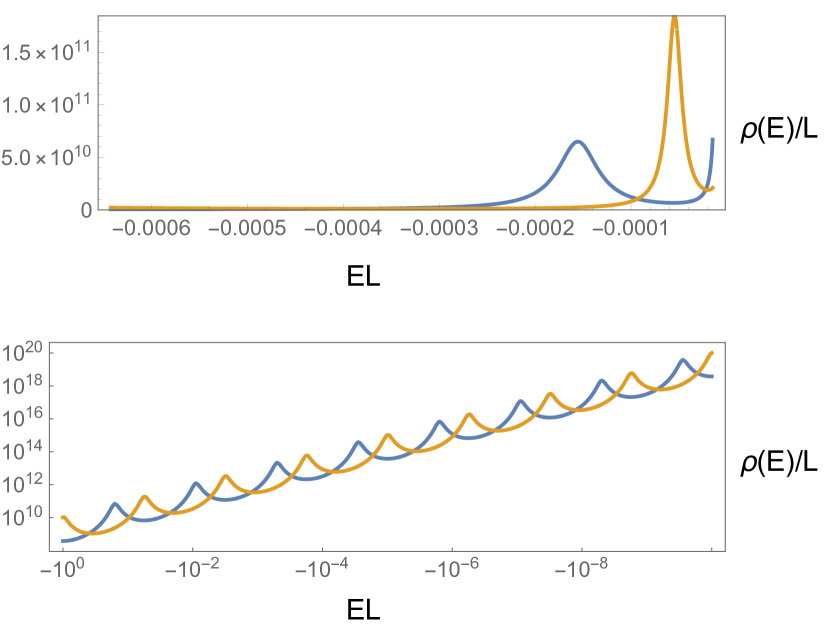
Figure 1: Density of states $\rho(E)$ of $H_{D}$ for $d=2$, $\beta=1.2>\beta_{c}$ and different angular momentum eigenstates. The yellow and blue curves correspond to the $m=0,-1$ angular momentum channels respectively. The boundary condition $h$ used here is the chiral boundary condition (3.16) which breaks parity. The parameter $L$ is the short distance cutoff taken here to be $0.195\mathrm{nm}$. The numeric values on both axis are in units of $\hbar c=0.197\,\mathrm{eV}\,\mu\mathrm{m}$. The set of pronounced peaks in both curves describes the quasi-bound spectrum in the overcritical regime $\beta>\beta_{c}$ as calculated in (3.11). The lower panel displays the detailed structure of the infinite geometric ladders of the quasi-bound states in a logarithmic scale. The $m=0,-1$ ladders are intertwined, indicative of the breaking of parity by the boundary condition. These results are independent of the specific choice of $L$ or $h$ (provided that it breaks parity).

Under (3.15), a solution of the Dirac equation with angular momentum $m$ obeying boundary condition (3.8) will transform into a different solution with angular momentum $-m-1$ obeying (3.8) with $h\to-h^{-1}$. Thus, the boundary condition respects parity if and only if

$$h_{m}=-h_{-m-1}^{-1}.$$ (3.17)

Thus case 1 above preserves parity while 2, 3, 4 break parity. If (3.17) holds, transformation (3.15) links between the $m\leftrightarrow-m-1$ eigenspace solutions. The lowest angular momentum subspaces correspond to orbital angular momentum $m=0,-1$. If (3.17) holds, then the two geometric ladders (3.11) associated with $m=0,-1$ are degenerate. The reason is that, as seen in (3.7), under (3.15)

$$a_{11} \to a_{12},\,a_{12}\to-a_{11},\,a_{21}\to a_{22},\,a_{22}\to-a_{21}$$

$$h \to-h^{-1}$$ (3.18)

which render $z_{0}$ in (3.10) and consequently $E_{0}$ invariant. Thus $E_{0,m=\pm 1/2}$ are identical in this case. If (3.17) does not hold, this symmetry is not enforced and the degeneracy between the ladders is broken.

The visualization of parity breaking is displayed in Fig. 1 where the density of states $\rho(E)$ of $H_{D}$ is plotted for the $m=0,-1$ channels and $\beta>\beta_{c}$. The boundary condition that was used in Fig. 1 is the chiral boundary condition (3.16) which breaks parity. Both curves exhibit an identical set of pronounced peaks condensing near $E=0^{-}$. These peaks describe quasi-bound states (3.11) and, accordingly, are arranged in a set of two geometric ladders. The separation between the ladder is a distinct signal of parity breaking.

3.3 Experimental realization

The CSI to DSI transition has recently received further validity and interest due to a detailed experimental observation in graphene [39]. In what follows, we summarize the results of this observation and emphasize its most significant features.

Graphene is a particularly interesting condensed matter system where $H_{D}$ is relevant (for $d=2$). The basic reason for this argument is that low energy excitations in graphene behave as a massless Dirac fermion field with a linear dispersion $E=\pm v_{F}\left|p\right|$ where the Fermi velocity $v_{F}\approx 10^{6}$ m/s appears instead of $c$ [42]. These characteristics have been extensively exploited to make graphene a useful platform to emulate specific features of quantum field theory, topology and quantum electrodynamics (QED) [32, 34, 35, 43, 44, 45, 46], since an effective fine structure constant $\alpha_{G}=e^{2}/\hbar v_{F}$ of order unity is obtained by replacing the velocity of light $c$ by $v_{F}$.

It has been shown that single-atom vacancies in graphene can host a local and stable charge [39, 47, 48]. This charge can be modified and measured at the vacancy site by means of scanning tunneling spectroscopy and Landau level spectroscopy [47]. The presence of massless Dirac excitations in the vicinity of the vacancy charge motivates the assumption that these will interact in a way that can be described by a massless Dirac Coulomb system. Particularly, the low energy spectral features of the charged vacancy would be the same as that of a tunable Coulomb source. The experimental results of [39] provide confirmation of this hypothesis as will be detailed below.

The measurements and data analysis presented below were carried out as follows: positive charges are gradually increased into an initially prepared single atom vacancy in graphene. Using a scanning tunneling microscope (STM) the differential conductance $dI/dV\left(V\right)$ through the STM tip is measured at each charge increment at the vacancy site. The conductance $dI/dV\left(V\right)$ is expected to be proportional to the local density of states of the system [39, 49]. Thus, quasi-bound states should also appear as pronounced peaks in the $dI/dV$ curves.

For low enough values of the charge, the differential conductance displayed in Fig. 2b, shows the existence of a single quasi-bound state resonance whose distance from the Dirac point increases with charge. The behaviour close to the Dirac point, is very similar to the theoretical prediction of the under-critical regime $\beta<\beta_{c}$ displayed in Fig. 2a. The $\beta$ value associated with the data of Fig. 2b is obtained from matching the position of the quasi-bound state with the theoretical model where the cutoff $L$ and the boundary condition $h$ are fixed model parameters that will be given later. The theoretical position of the under-critical quasi-bound state as a function of $\beta$ is displayed in Fig. 4 along with the positions of the peak extracted from measurements. The existence of a quasi-bound state does not contradict CSI of the undercritical phase since the absence of any states occurs only in the low energy limit.

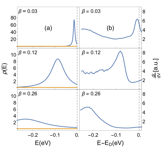
Figure 2: Experimental and theoretical picture in the undercritical regime. (a) Theoretical behaviour of the density of states $\rho(E)$ of the Dirac Hamiltonian $H_{D}$ in (3.1) with $d=2$, $c\to v_{F}=0.003c$ and angular momentum channels $m=-1$ (blue) and $m=0$ (yellow). The cutoff and boundary conditions are assigned here with the optimized values $L=0.195\,\mathrm{nm}$, $h=-0.85(m+1)$ as explained in the text. The $m=-1$ (blue) branch contains a single peak and the $m=0$ (yellow) branch shows no peak. While increasing $\beta$, the resonance shifts to lower energy and becomes broader. (b) The conductance $dI/dV$ measured at a single vacancy in graphene using STM as a function of the applied voltage $V$. The determination of the parameter $\beta$ is obtained from matching the position of the peak in the $dI/dV$ curve with the theoretical model where the cutoff $L$ and the boundary condition $h$ are fixed model parameters.

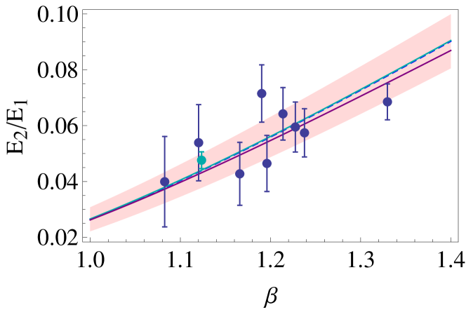
Figure 5: Comparison between the experimentally obtained $E_{2}/E_{1}$ ratio and the universal factor $e^{-\pi/\sqrt{\beta^{2}-1/4}}$. Blue points: the ratio $E_{2}/E_{1}$ obtained from the position of the points in Fig. 4. Green point: Universal Efimov energy ratio as measured in Caesium atoms [23, 31]. Blue line (dashed): the corresponding optimized curve, fitted according to the model $e^{-b/\sqrt{\beta^{2}-1/4}}$ and corresponding to $b=3.145$ with standard error of $\Delta b=0.06$ consistent with the predicted value $\pi$. The shaded pink region is the $\pm 2\Delta b$ confidence interval of the curve. Cyan line: universal low energy factor $e^{-\pi/\sqrt{\beta^{2}-1/4}}$. Purple line: theoretical ratio $E_{2}/E_{1}$ obtained from the exact solution of the Dirac equation. As $\beta\rightarrow 0.5$, $|E_{n}|$ becomes smaller therefore the green and purple curves coincide for low $\beta$. The error bar on the resonance energies is $\pm 1meV$.

At the point where the build up charge exceeds a certain value, three additional resonances emerge out of the Dirac point. These resonances are interpreted as the lowest overcritical $(\beta>1/2)$ resonances which we denote $E_{1},E^{\prime}_{1},E_{2}$ respectively. The corresponding theoretical and experimental behaviours displayed in Figs. 1, 3, show a very good qualitative agreement. To achieve a quantitative comparison solely based on the massless Dirac Coulomb Hamiltonian (3.13), the theoretical $\beta$ values corresponding to the respective positions of the lowest overcritical experimental resonance $E_{1}$ (as demonstrated in Fig. 3) are deduced for fixed $L$ and the boundary condition $h$ (as before). This allows to determine the lowest branch $E_{1}(\beta)$ represented in Fig. 4. Then, the experimental points $E^{\prime}_{1},E_{2}$ are now free points to be directly compared to their corresponding theoretical branch as seen in Fig. 4. Parameters $L$ and $h$, are determined according to the ansatz $h=a(m+1)$, and correspond to optimal values of $L=0.195\,\mathrm{nm}$, $a\simeq-0.85$. The comparison of the experimental $E_{2}/E_{1}$ ratio with the universal prediction $E_{n+1}/E_{n}=e^{-\pi/\sqrt{\beta^{2}-1/4}}$ is given in Fig. 5. A trend-line of the form $e^{-b/\sqrt{\beta^{2}-1/4}}$ is fitted to the ratios $E_{2}/E_{1}$ yielding a statistical value of $b=3.145$ with standard error of $\Delta b=0.06$ consistent with the predicted value $\pi$. An error of $\pm 1meV$ is assumed for the position of the energy resonances.

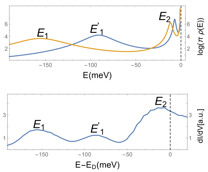
Figure 3: Experimental and theoretical picture in the overcritical regime. Upper plot: Theoretical behaviour of the low energy density of states $\rho(E)$ for overcritical $\beta=1.33$. The Blue (Yellow) line corresponds to $m=-1$ ($m=0$) orbital angular momentum. The peaks on the vertical scale describe the first quasi-bound states with two (Blue and Yellow) infinite geometric towers of states. Lower plot: Experimental values of the tunnelling conductance measured at the charged vacancy site in graphene.

A few further comments are appropriate:

1. The points on the $E_{2}(\beta)$ curve follow very closely the theoretical prediction $E_{n+1}/E_{n}=e^{-\pi/\sqrt{\beta^{2}-1/4}}$. This result is relatively insensitive to the choice of $h,L$.

2. In contrast, the correspondence between the $E^{\prime}_{1}\left(\beta\right)$ points and the theoretical branch is sensitive to the choice of $h,L$. This reflects the fact that while each geometric ladder is of the form (3.11), the energy scale $E_{0}$ is different between the $E_{1}\left(\beta\right)$ and $E^{\prime}_{1}\left(\beta\right)$ channels thus leading to a shifted relative position. The ansatz taken for $h$ is phenomenological, however, in order to get reasonable correspondence to theory, the explicit dependence on $m$ is needed. More importantly, it is necessary to use a parity breaking boundary condition (see section 3.2) to describe the $E^{\prime}_{1}(\beta)$ points, otherwise, both angular momentum channels $E_{1}\left(\beta\right)$, $E^{\prime}_{1}\left(\beta\right)$ will become degenerate and there would be no theoretical line to describe the $E^{\prime}_{1}\left(\beta\right)$ points. The existence of the experimental $E^{\prime}_{1}\left(\beta\right)$ branch is therefore a distinct signal that parity symmetry in the corresponding Dirac description is broken. In graphene, exchanging the triangular sub-lattices is equivalent to a parity transformation. Creating a vacancy breaks the symmetry between the two sub-lattices and is therefore at the origin of broken parity in the Dirac model.

3. The optimal value obtained for the short distance cutoff $L=0.195\,\mathrm{nm}$ is fully consistent with the low energy requirement $E_{1}L/\hbar v_{F}\simeq 0.03\ll 1$ necessary to be in the regime relevant to observe the $\beta$-driven QPT. Furthermore, it is quite close the lattice spacing of graphene ($\approx 0.15\,\mathrm{nm}$)

One of the most interesting features of observed quasi bound states is their similarity with the Efimov spectrum. As discussed in section 2.2, Efimov states are a geometric tower of states with a fixed geometric factor which is derived from an effective Schrödinger equation with a $V=-\lambda/r^{2}$ potential (as in (2.1)) and overcritical potential strength $\lambda=s_{0}+1/4$, $s_{0}\approx 1.00624$. To emphasize the similarities between the Dirac quasi bound spectrum and the Efimov spectrum or, more generally, between the CSI to DSI transition in the Dirac and Schrödinger Hamiltonians $H_{D}$, $H_{S}$, two additional experimental points (pink x’s) are presented in Fig. 4. These points are the values of Efimov energy states measured in Caesium atoms [23, 31] and scaled with an appropriate overall factor. The points are placed at the (overcritical) fixed Efimov value $\beta_{\mathrm{E}}=1.1236$ corresponding to the geometric factor of Efimov states. The universality of the transition is thereby emphasized in Fig. 4 in which curves calculated from a massless Dirac Hamiltonian, energy positions of tunneling conductance peaks in graphene and resonances of a gas of Caesium atoms are combined in a meaningful context.

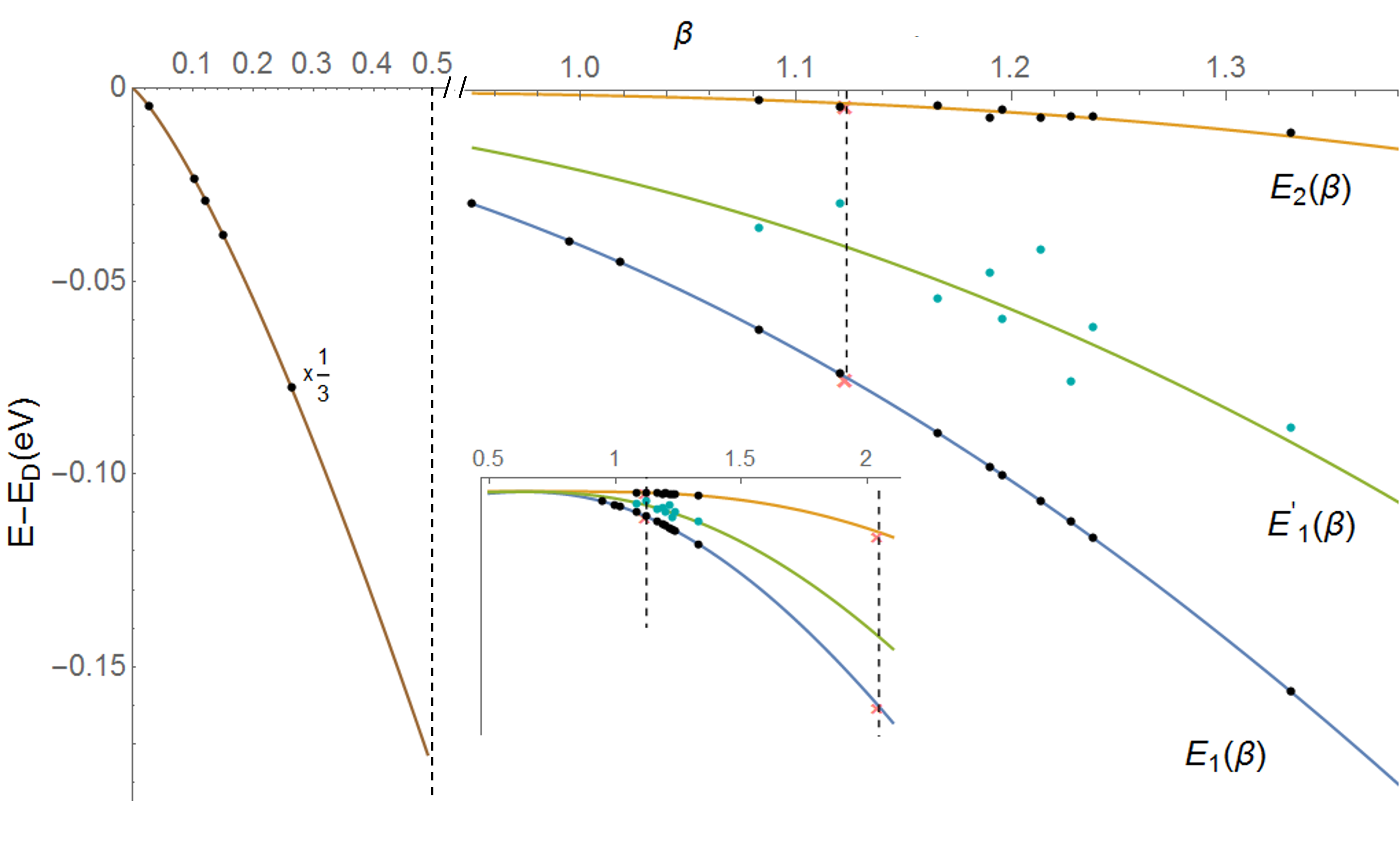
Figure 4: Comparison of lowest quasi bound state energy curves $E_{n}(\beta)$ with experimentally measured tunneling conductance peaks. The curves $E_{1}(\beta),E^{\prime}_{1}(\beta),E_{2}(\beta)$ describe resonances extracted from the density of states of the $m=0$ ($E_{1},\,E_{2}$) and $m=-1$ ($E^{\prime}_{1}$) angular momentum channels. $E_{1},\,E_{2}$ and $E^{\prime}_{1}$ are the first quasi bound states appearing for $\beta>1/2$ in the $m=0,-1$ channels respectively. The brown curve is the position of the single under-critical quasi bound state as a function of $\beta<\beta_{c}$ scaled by a factor of $1/3$ in the vertical axis. The black and cyan dots correspond to the positions of the tunneling conductance peaks as measured in graphene. The determination of the $\beta$ value associated with these points is obtained from matching the position of the single under-critical peak and first over-critical peak ($E_{1}$) in the $dI/dV$ curves with the theoretical model where the cutoff $L$ and boundary condition $h$ are fixed parameters. The two pink x’s are the values of Efimov energy states as measured in Caesium atoms [23, 31] and rescaled by an appropriate overall factor. These points corresponds to the (overcritical) fixed Efimov value $\beta_{\mathrm{E}}=1.1236$. Similarly, additional experimental points obtained in [24, 25] are displayed in the inset.

4 Relation to universality

In sections 2, 3 we obtained the properties of the CSI to DSI transition from a direct analysis of the corresponding eigenstates of each system. In what follows, we describe the same physics, but this time through the language of the renormalization group (RG). As will be detailed next, the description of this phenomenon in a RG picture provides a notable example of a case in which there is universality even in the absence of any fixed points. To understand this point more clearly, we first recall the physical meaning of the RG formalism and the usual context for which universality is understood with relation to RG.

Universality is a central concept of physics. It refers to phenomena for which very different systems exhibit identical behavior when properly coarse-grained to large distance (or low energy) scales. Important representatives of universality are systems that are close to a critical point, e.g., liquid-gas or magnetic systems. Near the critical point, these systems exhibit continuous scale invariance (as in (1.1)) where the free energy and correlation length vary as a power of the temperature (or some other control parameter). The exponents of these functions are real valued and are identical for a set of different systems thereby constituting a “universality class”.

The contemporary understanding of university in critical phenomena is provided by the tools of RG and effective theory. In the framework of the later, low energy physics is described by a Hamiltonian $H$ with a series of interaction terms $g_{n}\mathcal{O}_{n}$ constrained by symmetries. Intrinsic to this description is an ultraviolet cutoff $\Lambda$ reflecting the conceptual idea that $H$ is obtained from some microscopic Hamiltonian $H_{0}$ by integrating out degrees of freedom with length scale shorter than $1/\Lambda$. The dependence of $\vec{g}\equiv\left(g_{1},g_{2}\ldots\right)$ on $\Lambda$ defines the RG space of parameters $\vec{g}\left(\Lambda\right)$ which represent a large set of Hamiltonians $H\left(\vec{g}\left(\Lambda\right)\right)$. Within this picture, the scale invariant character of critical phenomena is attributed to the case where $H_{0}\left(\vec{g}_{0}\right)$ flows in the infrared limit, $\Lambda\rightarrow 0$, to $H\left(\vec{g}_{\ast}\right)$ where $\vec{g}_{\ast}$ is a fixed point. Additionally, universality classes arise since trajectories starting at distinct positions on RG space can flow to the same fixed point for $\Lambda\rightarrow 0$. The role of RG fixed points in the description of universality, effective theory and scale invariance is central and extends throughout broad sub-fields in physics.

4.1 Renomarlization group formalism for the Schrödinger $1/r^{2}$ potential

The RG picture which describes the low energy physics of the Schrödinger $-\lambda/r^{2}$ potential in the $\lambda>\lambda_{c}$ regime cannot be associated with a fixed point because of the absence of CSI. However, even without fixed points, we expect universality to appear in this regime since the geometric series factor $E_{n+1}/E_{n}$ = $\exp\left(-2\pi/\sqrt{\lambda-\lambda_{c}}\right)$ is independent of the short distance parameters associated with the cutoff $L$ and the boundary condition $g$

To see this explicitly [7, 13, 14, 15, 19], consider the radial Schrödinger equation for $H_{S}$ given by

$$-\left(\frac{d^{2}}{dr^{2}}+\frac{d-1}{r}\frac{d}{dr}-\frac{l(l+d-2)}{r^{2}}\right)-\frac{\lambda}{r^{s}}\psi\left(r\right)=E\psi\left(r\right),\hskip 10.00002ptL<r<\infty$$ (4.1)

where $\psi\left(r\right)$ is the radial wavefunction, $l$ the orbital angular momentum, $d$ the space dimension, $L$ a short distance cutoff and $s=2$ but remains implicit for a reason that will be clear shortly. A well defined eigenstate of (4.1) is obtained by imposing a boundary condition at $r=L$

$$L\frac{\psi^{\prime}\left(L\right)}{\psi\left(L\right)}=g,$$ (4.2)

$g\in\mathbb{R}$, which encodes the short-distance physics. To initiate a RG transformation we transform

$$L\rightarrow L+dL\equiv\epsilon L\,;\hskip 10.00002pt0<\epsilon-1\ll 1$$ (4.3)

and obtain an equivalent effective description with the short distance cut-off $\epsilon L$ and correspondingly, a new boundary condition at $r=\epsilon L$:

$$\epsilon L\frac{\psi^{\prime}\left(\epsilon L\right)}{\psi\left(\epsilon L\right)} = g\left(\epsilon L\right).$$ (4.4)

As a result of (4.3), equation (4.1) is now defined in the range $\epsilon L\leq r<\infty$ with the same functional form. With the help of the rescaling $r^{\prime}\equiv\epsilon^{-1}r,\,E^{\prime}\equiv\epsilon^{2}E$, equation (4.1) is modified to the equivalent form

$$-\left(\frac{d^{2}}{dr^{\prime 2}}+\frac{d-1}{r^{\prime}}\frac{d}{dr^{\prime}}-\frac{l(l+d-2)}{r^{\prime 2}}\right)-\frac{\lambda\epsilon^{2-s}}{r^{\prime s}}\psi\left(r^{\prime}\right)=E^{\prime}\psi\left(r^{\prime}\right)\hskip 10.00002ptL<r^{\prime}<\infty.$$ (4.5)

Thus, transformation (4.3) is accounted in (4.1) by $\lambda\to\lambda\epsilon^{2-s}$ and using (4.3) leads to the infinitesimal form

$$L\frac{d\lambda}{dL}=\left(2-s\right)\lambda.$$ (4.6)

Similarly, $g\left(\epsilon L\right)$ in (4.4) can be related to $g\left(L\right)$ as follows. The series expansion of $g\left(\epsilon L\right)$ in $\epsilon-1$ is

$$g\left(\epsilon L\right)=L\frac{\psi^{\prime}\left(L\right)}{\psi\left(L\right)}+\left(\epsilon-1\right)\left(L\frac{\psi^{\prime}\left(L\right)}{\psi\left(L\right)}-L^{2}\left(\frac{\psi^{\prime}\left(L\right)}{\psi\left(L\right)}\right)^{2}+L^{2}\frac{\psi^{\prime\prime}\left(L\right)}{\psi\left(L\right)}\right)+\mathcal{O}\left(\epsilon-1\right)^{2}.$$ (4.7)

Manipulation of (4.7) by insertion of the radial Schrödinger equation (4.1) and the definition of $g\left(L\right)$ yield

$$g\left(\epsilon L\right)=g\left(L\right)+\left(\epsilon-1\right)\left(\left(2-d\right)g\left(L\right)-g\left(L\right)^{2}-\lambda L^{2-s}+l(l+d-2)-L^{2}E\right)$$ (4.8)

where terms of order $\left(\epsilon-1\right)^{2}$ or higher were eliminated. The equivalent differential form is thus

$$L\frac{dg}{dL}=\left(2-d\right)g-g^{2}-\lambda L^{2-s}+l(l+d-2)-L^{2}E.$$ (4.9)

In the low energy regime

$$L^{2}\left|E\right|\ll\left|\lambda-l(l+d-2)\right|$$ (4.10)

equation (4.9) reduces to

$$L\frac{dg}{dL}=\left(2-d\right)g-g^{2}-\lambda$$ (4.11)

where the orbital angular momentum was taken to be $l=0$ and $s$ set to $s=2$ for brevity. Finally, the combination of (4.6), (4.11) constitutes the RG equations

$$\beta\left(\lambda\right)\equiv L\frac{d\lambda}{dL} = \left(2-s\right)\lambda$$

$$\beta\left(g\right)\equiv L\frac{dg}{dL} = -\left(g-g_{+}\right)\left(g-g_{-}\right)$$ (4.12)

where

$$g_{\pm}=\frac{2-d}{2}\pm\sqrt{\lambda_{c}-\lambda}$$ (4.13)

and $\lambda_{c}=\left(d-2\right)^{2}/4$.

Since $\beta\left(\lambda\right)=0$ for $s=2$, $\lambda\left(L\right)$ remains unchanged under the RG transformation. In contrary, the function $\beta\left(g\right)$ is not trivial and has two roots $g_{\pm}$ . For $\lambda<\lambda_{c}$, the two roots correspond to two fixed points, $g_{-}$ unstable and $g_{+}$ stable. However, as $\lambda$ increases, the two fixed points get closer and merge for $\lambda=\lambda_{c}$. For $\lambda>\lambda_{c}$, $g_{\pm}$ become complex valued and the two fixed points vanish as can be seen in Fig. 6a. The solution for $g\left(L\right)$ in this regime is given explicitly by (see Fig. 6b)

$$g\left(L\right)=\frac{2-d}{2}-\sqrt{\lambda-\lambda_{c}}\tan\left[\sqrt{\lambda-\lambda_{c}}\ln\left(L/L_{0}\right)-\phi_{g}\right]$$ (4.14)

where $\phi_{g}\equiv\arctan\left(\frac{g_{0}-\frac{2-d}{2}}{\sqrt{\lambda-\lambda_{c}}}\right)$. Unlike the case of a fixed point, the flow of $g\left(L\right)$ in (4.14) does not terminate at any specific point but rather oscillate periodically in $\log L$ with period $L\to e^{\pi/\sqrt{\lambda-\lambda_{c}}}L$ independent of the initial condition $g\left(L_{0}\right)=g_{0}$.

The appearance of two fixed points for $\lambda<\lambda_{c}$, which annihilate at $\lambda_{c}$ and give rise to a log-periodic flow for $\lambda>\lambda_{c}$ is the transcription of the CSI to DSI transition in the RG picture. The periodicity $e^{\pi/\sqrt{\lambda-\lambda_{c}}}$, being independent on the initial conditions, $g\left(L_{0}\right)=g_{0}$, represents a universal content even in the absence of fixed points.

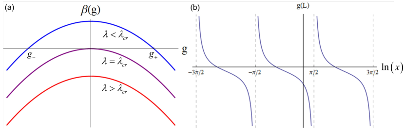
Figure 6: Visualization of the renormalization group picture associated with the boundary condition $g(L)$ at the short distance cutoff $r=L$ for the case of the Schrödinger $V\left(r\right)=-\lambda/r^{2}$ potential $H_{S}$. (a) The $\beta\left(g\right)$ function in the over-critical and under-critical regimes. For $\lambda<\lambda_{c}$, $\beta\left(g\right)$ has two roots correspond to two fixed points, $g_{-}$ unstable and $g_{+}$ stable. The point $\lambda=\lambda_{c}$ is a transition point where the roots merge into a single fixed point. For $\lambda>\lambda_{c}$ there are no real fixed points. (b) The behaviour of the boundary condition $g\left(L\right)$ in the overcritical regime $\lambda>\lambda_{c}$ and $d=3$ as a function of $\ln\left(x\right)$ with $x\equiv\sqrt{\lambda-\lambda_{c}}\ln\left(L/L_{0}\right)-\phi_{g}$, $\phi_{g}\equiv\arctan\left(\frac{g_{0}-\frac{2-d}{2}}{\sqrt{\lambda-\lambda_{c}}}\right)$. Independent of the initial condition $g_{0}\left(L_{0}\right)$, $g\left(L\right)$ is a log-periodic function of $L$ which, as shown in (1.3), is a generic feature of DSI.

An analogue of the RG equations (4.12) can be derived for the boundary condition $h\left(L\right)$ in (3.8) of the massless Dirac Coulomb system described in section 3 [50].

5 Discussion

The similarities between the Dirac and Schrödinger system $H_{S},H_{D}$

$$H_{S} = p^{2}-\lambda/r^{2}$$ (5.1)

$$H_{D} = \gamma^{0}\gamma^{j}p_{j}-\beta/r$$ (5.2)

presented in sections 2, 3 motivate the study of whether a similar transition from CSI to DSI is possible for a generic class of systems and, if so, what are the common ingredients within this class. Below we briefly survey some other setups which interestingly give rise to a CSI to DSI transition. The relation between all these cases is summarized in table 2.

Table 2: Comparison between the various cases discussed in the text for which a transition between a continuous scale invariant phase and a discrete scale invariant phase occurs. In the DSI regime each system is characterized by the sudden appearance of a geometric tower of modes with the universal form $O_{n}=O_{0}\,\exp\left(-b\frac{\pi n}{\sqrt{x-x_{c}}}\right)$. In lines 1–3 of the table, $O_{n}$ are one body bound states. Lines 4–5 describe many body quantum systems where $O_{n}$ are fermion masses and 3-body bound states respectively. Line 6 provides a comparison with the Berezinskii-Kosterlitz-Thouless phase transition where the analog quantity for $O_{n}$ is the free energy $F$ for $T\gtrsim T_{c}$. In line 4, $\alpha_{N}$ is a $N$ dependent real number whose exact value can be found in [51]. In line 5, $c_{-}$ is a $d$ dependent real positive number defined in section 5.3.

System	$O_{n}$	$x$	$x_{c}$	$b$
$H_{S}=p^{2}-\lambda/r^{2}$	$E_{n}$	$\lambda$	$\left(d-2\right)^{2}/4$	$2$
$H_{D}=\gamma^{0}\gamma^{j}p_{j}-\beta/r$	$E_{n}$	$\beta^{2}$	$\left(d-1\right)^{2}/4$	$1$
$H_{L}=\left(-\dfrac{d^{2}}{dx^{2}}\right)^{N}-\dfrac{\lambda_{L}}{x^{2N}}$	$E_{n}$	$\lambda_{L}$	$\left(\dfrac{(2N-1)!!}{2^{N}}\right)^{2}$	$N\alpha_{N}$
QED3 with $N$ massless flavours	$m_{n}$	$N^{-1}$	$\pi^{2}/32$	$\pi/\sqrt{8}$
Efimov effect in $d$ dimensions	$E_{n}$	$d$	$2.3$	$1/c_{\pm}\left(d\right)$
BKT	$F$	$T$	$T_{c}$	system dependent

5.1 Lifshitz scaling symmetry

Since $H_{S}$ and $H_{D}$ share the property that the power law form of the corresponding potential matches the order of the kinetic term, it is interesting to examine whether this property is a sufficient ingredient by considering a generalized class of one dimensional Hamiltonians,

$$H_{L}=\left(-\frac{d^{2}}{dx^{2}}\right)^{N}-\frac{\lambda_{L}}{x^{2N}},$$ (5.3)

where $N$ is a natural integer and $\lambda_{L}$ a real valued coupling. The Hamiltonian $H_{L}$ describes a quantum system with non-quadratic anisotropic scaling between space and time for $N>1$. This so called “Lifshitz scaling symmetry” [52], manifest in (5.3), can be seen for example at the finite temperature multicritical points of certain materials [53, 54] or in strongly correlated electron systems [55, 56, 57]. Quartic dispersion relations $E\sim p^{4}$ can also be found in graphene bilayers [58] and heavy fermion metals [59]. It may also have applications in particle physics [52], cosmology [60] and quantum gravity [61, 62, 63].

The detailed solution of the corresponding Schrödinger equation $H_{L}\psi=E\psi$ [51] confirms that a transition from CSI to DSI occurs at $\lambda_{L,c}=\left(2N-1\right)!!^{2}/2^{2N}$, $\forall N\geq$1. The CSI phase contains no low energy, $\left|E\right|^{1/2N}L\ll 1$ ($L$ is a short distance cutoff), bound states and the DSI phase is characterized by an infinite set of bound states forming the geometric series

$$E_{n}=-E_{0}e^{-\frac{N\alpha_{N}\pi n}{\sqrt{\lambda_{L}-\lambda_{L,c}}}},\,\,0<\lambda_{L}-\lambda_{L,c}\ll 1$$ (5.4)

where $E_{0}>0$ and $\alpha_{N}$ is an $N$ dependent real number. For $\lambda_{L}-\lambda_{L,c}\to 0^{+}$, the analytic behavior of the spectrum is characteristic of the Berezinskii-Kosterlitz-Thouless (BKT) scaling in analogy with the $N=1$ case. However, unlike the $N=1$ case, the BKT scaling appears only for $\lambda_{L}-\lambda_{L,c}\to 0^{+}$. Deeper in the overcritical regime, the dependence on $\left(\lambda_{L}-\lambda_{L,c}\right)^{1/2}$ in (5.4) is replaced by a more complicated function of $\lambda_{L}-\lambda_{L,c}$ [51]. The transition as well as the value of $\lambda_{L,c}$ is independent of the short distance physics characterized by the boundary conditions and cutoff $L$.

Since $H_{L}$ is a high order differential operator it requires the specification of several $x=L$ boundary condition parameters (unlike the one parameter $g$ in section 2.1) in order to render it as a well defined self-adjoint operator on the interval $L<x<\infty$. The most general choice of boundary conditions is parameterized by a unitary $N\times N$ matrix. Accordingly, the corresponding $N^{2}$ dimensional RG space is characterized by fixed points in the under-critical regime $\lambda_{L}<\lambda_{L,c}$. Interestingly, the DSI over-critical regime $\lambda_{L}>\lambda_{L,c}$ is not filled with an infinite number of cyclic flows such as represented in Fig. 6b. Instead, there is a ’limit cycle’ [64], i.e., an isolated closed trajectory at which flows terminate [65] (see Fig. 7).

5.2 QED in $2+1$ dimensions and $N$ fermionic flavors

The study of dynamical fermion mass generation in $2+1$ dimensional quantum electrodynamics (QED) [66, 67] provides an interesting many body instance of the CSI to DSI transition. Consider the $2+1$ dimensional QED Lagrangian

$$\mathcal{L}=i\bar{\Psi}\gamma^{\mu}\left(\partial_{\mu}-ieA_{\mu}\right)\Psi-\frac{1}{4}F_{\mu\nu}F^{\mu\nu}$$ (5.5)

where $\Psi$ is a vector of $N$ identical types of fermion fields with zero mass. In this theory, $e^{2}$ or alternatively $\alpha\equiv Ne^{2}/8$, is a dimension-full coupling. Analogous to the short distance cutoff $L$ of sections 2, 3, 5.1, $\alpha$ constitutes the only energy scale of the theory. Consequently, the low energy regime $E\ll\alpha$ can be shown to exhibit CSI.

The understand whether or not fermion mass appears as a result of quantum fluctuations it is required to calculate the fermion propagator, specifically, the self-energy $\Sigma\left(p\right)$. Under a particular (non-perturbative) approximation scheme [66], the expression for $\Sigma\left(p\right)$ can be extracted from the solution of the following differential equation

$$-\Sigma^{\prime\prime}\left(p\right)-\frac{2}{p}\Sigma^{\prime}\left(p\right)-\frac{\lambda_{Q}}{p^{2}+\Sigma\left(p\right)^{2}}\Sigma\left(p\right)=0,\hskip 5.0pt0<p<\alpha$$ (5.6)

with boundary condition

$$\alpha\frac{\Sigma^{\prime}\left(\alpha\right)}{\Sigma\left(\alpha\right)}=-1$$ (5.7)

where $\lambda_{Q}\equiv 8/\left(\pi^{2}N\right)$. Close to a transition point the fermion mass and thereby $\Sigma\left(p\right)$ are non-zero but arbitrarily small such that $\Sigma\left(p\right)\ll p<\alpha$. As a result, (5.6) can be further approximated by assuming $\Sigma\left(p\right)^{2}$ in the denominator is a constant which we define as $\Sigma\left(p\right)^{2}\to m^{2}/\lambda_{Q}$. Expanding to order $m^{2}$ yields

$$-\Sigma^{\prime\prime}\left(p\right)-\frac{2}{p}\Sigma^{\prime}\left(p\right)-\frac{\lambda_{Q}}{p^{2}}\Sigma\left(p\right)=-\frac{m^{2}}{p^{4}}\Sigma\left(p\right).$$ (5.8)

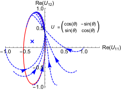
Figure 7: A two dimensional projection of the (four dimensional) RG picture of the system $H=d_{x}^{4}-2/x^{4}$. The four boundary conditions at $x=L$ are parametrized by a unitary $2\times 2$ matrix $U$. The initial conditions for the dashed blue flows are specified by choosing $\theta=-\pi,\ldots,-\pi/10,0$ for the $U$ matrix as displayed. All the trajectories flow towards a limit cycle. There exists a non-unitary fixed point, denoted by the blue cross, which is enclosed by the cycle when projected down onto any two dimensional subspace.

A closer look on equations (5.7), (5.8) reveals that they are the same as the radial form of the Schrödinger equation with a $V=-\lambda/r^{2}$ potential

$$-\left(\frac{d^{2}}{dr^{2}}+\frac{d-1}{r}\frac{d}{dr}-\frac{l(l+d-2)}{r^{2}}\right)-\frac{\lambda}{r^{2}}\psi\left(r\right) = -k^{2}\psi\left(r\right),\hskip 5.0ptL<r<\infty$$ (5.9)

$$L\frac{\psi^{\prime}\left(L\right)}{\psi\left(L\right)} = g$$ (5.10)

where $k=\sqrt{-E}$ as described in section 2 and in equations (4.1), (4.2). To see this explicitly, we rewrite (5.7), (5.8) in terms of $r\equiv 1/p$, $\psi\left(r\right)\equiv\Sigma\left(p\right)$, $L\equiv 1/\alpha$ which then yields

$$-\psi^{\prime\prime}(r)-\frac{\lambda_{Q}}{r^{2}}\psi(r) = -m^{2}\psi(r),\hskip 5.0ptL<r<\infty$$ (5.11)

$$L\frac{\psi^{\prime}\left(L\right)}{\psi\left(L\right)} = 1.$$ (5.12)

Thus, the appearance of a non-vanishing fermion self energy constitutes a system of the form (5.9), (5.10) with $d=1,\,\lambda=\lambda_{Q}$ and $g=1$. The resulting implication is that a transition from a CSI to DSI occurs at $\lambda_{Q,c}=1/4$. For $\lambda_{Q,c}<1/4$ there will be no $\Sigma\left(p\right)\neq 0$ solution for the self-energy in the $m/\alpha\ll 1$ regime. However, once $\lambda_{Q}$ exceeds $\lambda_{Q,c}=1/4$ an infinite geometric tower of possible non-trivial self-energy solutions appears with eigenvalues

$$m_{n+1}/m_{n}=e^{-\frac{\pi}{\sqrt{\lambda_{Q}-\lambda_{Q,c}}}}.$$ (5.13)

The critical point $\lambda_{Q,c}=1/4$ corresponds to a critical fermion number $N_{c}=32/\pi^{2}$ for which the DSI regime is $N<N_{c}$. In these term, (5.13) reduces to

$$m_{n+1}/m_{n}=e^{-\frac{\pi}{\sqrt{\frac{1}{N}-\frac{\pi^{2}}{32}}}\pi/\sqrt{8}}.$$ (5.14)

5.3 Efimov effect in $d$ dimensions

As described in 2.2, the Efimov effect [3, 4, 22] is a remarkable phenomenon in which three particles form an infinite geometric ladder of low energy bound states. The effect occurs when at least two of the three pairs interact with a range that is small compared to the scattering length. It can be shown that the Efimov effect is possible only for space dimensions $2.3<d<3.76$ [68] which essentially limits the phenomenon to 3 dimensions. Interestingly, in the case where $d$ is allowed to be tuned continuously, two CSI to DSI transitions are initiated at the critical dimensions $d_{-}=2.3$, $d_{+}=3.76$ [69]. In what follows we outline the main features of this result.

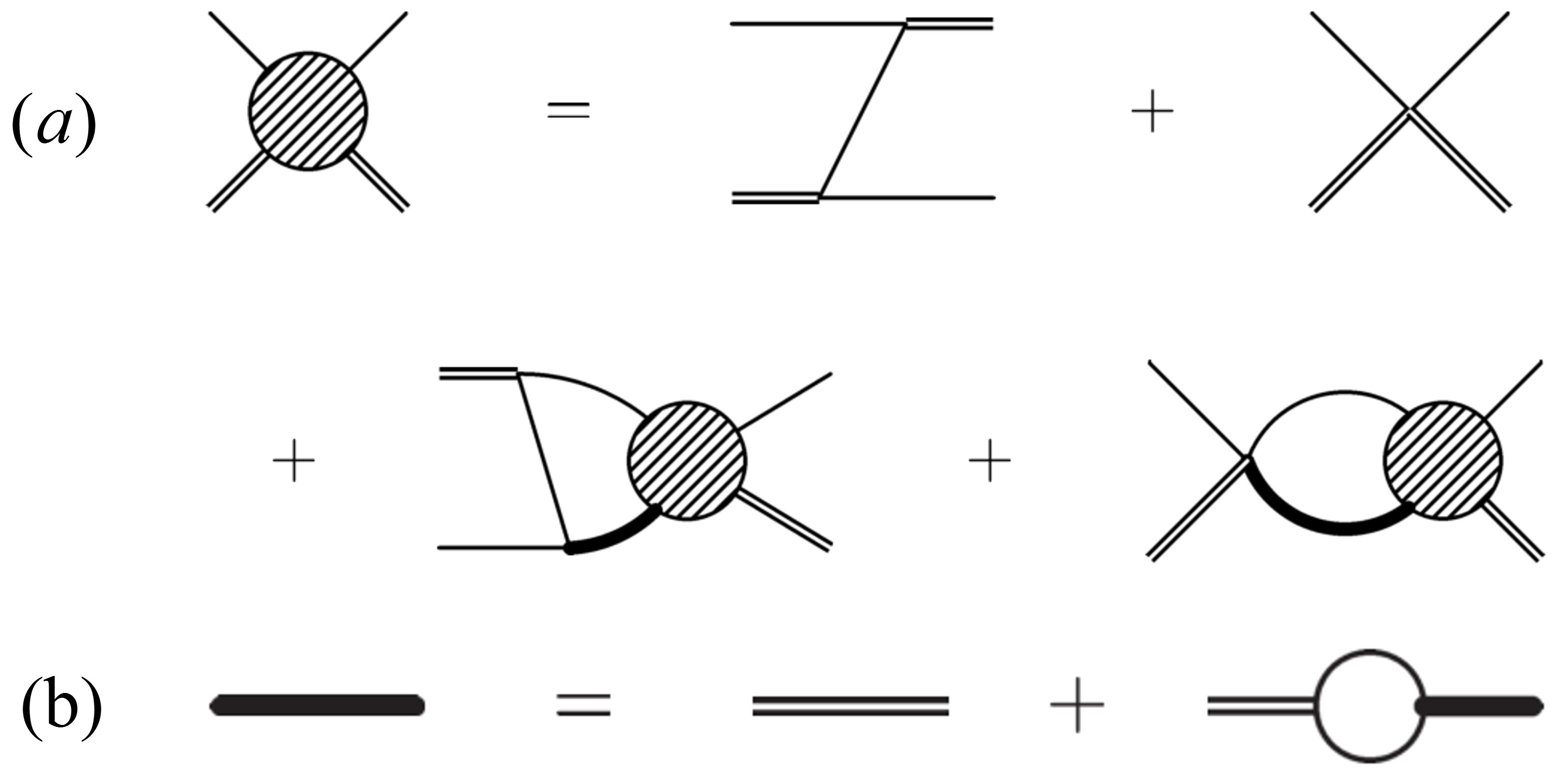
Figure 8: Diagrammatic representation of the atom-diatom scattering amplitude and the diatom propagator [22]. (a) Diagrammatic self-consistent equation for the atom-diatom scattering amplitude. (b) Diagrammatic self-consistent equation for the diatom field propagator.

Low energy 3-body observables of locally interacting identical bosons can be described by an effective field theory with Lagrangian

$$\mathcal{L}=\psi^{\dagger}\left(i\frac{\partial}{\partial t}+\frac{1}{2}\nabla^{2}\right)\psi+\frac{g_{2}}{4}\left(\Delta^{\dagger}\Delta\right)-\frac{g_{2}}{4}\left(\Delta^{\dagger}\psi^{2}+\psi^{\dagger^{2}}\Delta\right)-\frac{g_{3}}{36}\left(\Delta^{\dagger}\Delta\psi^{\dagger}\psi\right)$$ (5.15)

where $\psi$ is a non-relativistic bosonic atom field, $\Delta$ is a non dynamical ’diatom’ field annihilating two atoms at one point and $g_{2}$, $g_{3}$ are bare 2-body and 3-body couplings respectively. With the diatom field and these interaction terms, it is possible to reproduce the physics of the Efimov effect [70]. The main ingredient of this procedure is the diagramatic calculation of the atom-diatom scattering amplitude as shown in Fig. 8. The self-consistent equations described in Fig. 8 leads to the following approximate relation for the s-wave atom-diatom amplitude $A_{s}$

$$A_{s}\left(p\right)=-\left(\frac{4}{3}\right)^{\frac{d-2}{2}}\frac{4\sin\left(\frac{d}{2}\pi\right)}{\pi}\int_{0}^{\infty}\,dq\frac{q}{p^{2}+q^{2}}\,{}_{2}F_{1}\left(\begin{matrix}\frac{1}{2}&&1\\ &\frac{d}{2}\end{matrix};\frac{p^{2}q^{2}}{p^{2}+q^{2}}\right)A_{s}\left(q\right)$$ (5.16)

Since there are no dimension-full parameters in (5.16) we are, once again, faced with a CSI equation, in analogy with the characteristics of equations (2.2), (3.3), (5.3) and (5.8). By inserting the ansatz $A_{s}\left(p\right)=p^{s-1}$, two possible solutions for (5.16) are obtained

$$A_{s}\approx a_{1}p^{\sqrt{s^{2}}-1}+a_{2}p^{-\sqrt{s^{2}}-1}$$ (5.17)

where $s^{2}\left(d\right)$ is a solution of the $s\to-s$ invariant equation

$$2\sin\left(\frac{d\pi}{2}\right){}_{2}F_{1}\left(\begin{matrix}\frac{d-1+s}{2}&&\frac{d-1-s}{2}\\ &\frac{d}{2}\end{matrix};\frac{1}{4}\right)+\cos\left(\frac{s}{2}\pi\right)=0.$$ (5.18)

The numerical solution $s^{2}\left(d\right)$ of (5.18) shows that near $d=d_{\pm}$, $s^{2}\left(d_{\pm}\right)=0$, $\partial_{d}s^{2}\left(d_{-}\right)<0$, $\partial_{d}s^{2}\left(d_{+}\right)>0$ and it is analytic. Consequently, near the critical dimensions $d_{\pm}$

$$s^{2}\left(d\right)=\pm c_{\pm}^{2}\left(d-d_{\pm}\right)+\mathcal{O}\left(d-d_{\pm}\right)$$ (5.19)

with $c_{\pm}>0$. The insertion of (5.19) into (5.17) imply a CSI to DSI transition from real to complex valued power law behaviour of $A_{s}$. The DSI regime $d_{-}<d<d_{+}$ is consistent with the strip within which the Efimov states appear. Consequently, close to the critical points $d=d_{\pm}$, $A_{s}\left(p\right)$ in (5.17) obeys the following DSI scaling relation (as in (1.1))

$$A_{s}\left(e^{\frac{\pi n}{c_{\pm}\sqrt{|d-d_{\pm}|}}}p\right)=e^{-\frac{\pi n}{c_{\pm}\sqrt{|d-d_{\pm}|}}}A_{s}\left(p\right).$$ (5.20)

The corresponding RG equation for the couplings is

$$\Lambda\frac{d}{d\Lambda}G=\frac{1-s^{2}\left(d\right)}{2}\left(G-G_{-}\right)\left(G-G_{+}\right)$$ (5.21)

where $G\left(\Lambda\right)\equiv\Lambda^{2}g_{3}\left(\Lambda\right)/9g_{2}\left(\Lambda\right)^{2}$, $\Lambda$ is a UV cutoff and

$$G_{\pm}\equiv-\left(1\pm\sqrt{s^{2}\left(d\right)}\right)/\left(1\mp\sqrt{s^{2}\left(d\right)}\right).$$ (5.22)

In accordance with the RG picture detailed in section 4.1, the insertion of (5.19) shows that the $\beta$-function of $G$ contains two fixed points outside the strip $d_{-}<d<d_{+}$ which annihilate at $d=d_{\pm}$.

6 Summary

The breaking of continuous scale invariance (CSI) into discrete scale invariance (DSI) is a rich phenomenon with roots in multiple fields in physics. Theoretically, this transition plays an important role in various fundamental quantum systems such as the inverse-squared potential (section 2), the massless hydrogen atom (section 3), $2+1$ dimensional quantum electrodynamics (section 5.2) and the Efimov effect (sections 2.2 and 5.3). This CSI to DSI transition constitutes a quantum phase transition which appears for single body and strongly coupled many body systems and extends through non-relativistic, relativistic and Lifshitz dispersion relations. In a RG picture the transition describes universal low energy physics without fixed points and constitutes a physical realization of a limit cycle. Remarkably, the features of this transition have been measured recently in various systems such as cold atoms, graphene and Fermi gases [71]. In the DSI phase, the dependence of the geometric ladder of states on the control parameter (see Table 2) is in the class of Berezinskii-Kosterlitz-Thouless transitions. This provides an interesting, yet to be studied, bridge between DSI and two dimensional systems associated with BKT physics.

The characteristics described above provide the motivation to further study the ingredients associated with CSI to DSI transitions and we expect that these transitions will have an increasingly important role across the physics community in the future.

References

- Case [1950] K. M. Case, Phys. Rev. 80, 797 (1950).
- Landau [1991] L. D. Landau, Quantum mechanics : non-relativistic theory (Butterworth-Heinemann, Oxford Boston, 1991).
- Efimov [1970] V. Efimov, Physics Letters B 33, 563 (1970).
- Efimov [1971] V. Efimov, Sov. J. Nucl. Phys 12, 589 (1971).
- Lévy-Leblond [1967] J.-M. Lévy-Leblond, Phys. Rev. 153, 1 (1967).
- Camblong et al. [2001] H. E. Camblong, L. N. Epele, H. Fanchiotti, and C. A. Garcia Canal, Phys.Rev.Lett. 87, 220402 (2001), arXiv:hep-th/0106144 [hep-th] .
- Kaplan et al. [2009] D. B. Kaplan, J.-W. Lee, D. T. Son, and M. A. Stephanov, Phys. Rev. D 80, 125005 (2009).
- Nisoli and Bishop [2014] C. Nisoli and A. R. Bishop, Phys. Rev. Lett. 112, 070401 (2014).
- De Martino et al. [2014] A. De Martino, D. Klöpfer, D. Matrasulov, and R. Egger, Phys. Rev. Lett. 112, 186603 (2014).
- Jackiw [1995] R. W. Jackiw, Diverse topics in theoretical and mathematical physics (World Scientific, 1995).
- Meetz [1964] K. Meetz, Il Nuovo Cimento (1955-1965) 34, 690 (1964).
- Gitman et al. [2012] D. M. Gitman, I. Tyutin, and B. L. Voronov, Self-adjoint Extensions in Quantum Mechanics: General Theory and Applications to Schrödinger and Dirac Equations with Singular Potentials, Vol. 62 (Springer, 2012).
- Albeverio et al. [1981] S. Albeverio, R. Høegh-Krohn, and T. T. Wu, Phys. Lett. A 83, 105 (1981).
- Beane et al. [2001] S. R. Beane, P. F. Bedaque, L. Childress, A. Kryjevski, J. McGuire, and U. van Kolck, Phys. Rev. A 64, 042103 (2001).
- Mueller and Ho [2004] E. J. Mueller and T.-L. Ho, arXiv preprint cond-mat/0403283 (2004).
- Braaten and Phillips [2004] E. Braaten and D. Phillips, Phys. Rev. A 70, 052111 (2004).
- Hammer and Swingle [2006] H.-W. Hammer and B. G. Swingle, Annals of Physics 321, 306 (2006).
- Moroz and Schmidt [2010] S. Moroz and R. Schmidt, Annals of Physics 325, 491 (2010).
- Kolomeisky and Straley [1992] E. B. Kolomeisky and J. P. Straley, Phys. Rev. B 46, 12664 (1992).
- Jensen [2011] K. Jensen, Phys. Rev. Lett. 107, 231601 (2011), arXiv:1108.0421 [hep-th] .
- Jensen et al. [2010] K. Jensen, A. Karch, D. T. Son, and E. G. Thompson, Phys. Rev. Lett. 105, 041601 (2010), arXiv:1002.3159 [hep-th] .
- Braaten and Hammer [2006] E. Braaten and H.-W. Hammer, Physics Reports 428, 259 (2006).
- Kraemer et al. [2006] T. Kraemer, M. Mark, P. Waldburger, J. Danzl, C. Chin, B. Engeser, A. Lange, K. Pilch, A. Jaakkola, H.-C. Nägerl, et al., Nature 440, 315 (2006).
- Tung et al. [2014] S.-K. Tung, K. Jiménez-García, J. Johansen, C. V. Parker, and C. Chin, Phys. Rev. Lett. 113, 240402 (2014).
- Pires et al. [2014] R. Pires, J. Ulmanis, S. Häfner, M. Repp, A. Arias, E. D. Kuhnle, and M. Weidemüller, Phys. Rev. Lett. 112, 250404 (2014).
- Pollack et al. [2009] S. E. Pollack, D. Dries, and R. G. Hulet, Science 326, 1683 (2009).
- Gross et al. [2009] N. Gross, Z. Shotan, S. Kokkelmans, and L. Khaykovich, Phys. Rev. Lett. 103, 163202 (2009).
- Lompe et al. [2010] T. Lompe, T. B. Ottenstein, F. Serwane, A. N. Wenz, G. Zürn, and S. Jochim, Science 330, 940 (2010).
- Nakajima et al. [2011] S. Nakajima, M. Horikoshi, T. Mukaiyama, P. Naidon, and M. Ueda, Phys. Rev. Lett. 106, 143201 (2011).
- Kunitski et al. [2015] M. Kunitski, S. Zeller, J. Voigtsberger, A. Kalinin, L. P. H. Schmidt, M. Schöffler, A. Czasch, W. Schöllkopf, R. E. Grisenti, T. Jahnke, D. Blume, and R. Dörner, Science 348, 551 (2015).
- Huang et al. [2014] B. Huang, L. A. Sidorenkov, R. Grimm, and J. M. Hutson, Phys. Rev. Lett. 112, 190401 (2014).
- Miransky [1980] V. Miransky, Physics Letters B 91, 421 (1980).
- Pereira et al. [2007] V. M. Pereira, J. Nilsson, and A. H. Castro Neto, Phys. Rev. Lett. 99, 166802 (2007).
- Shytov et al. [2007a] A. V. Shytov, M. I. Katsnelson, and L. S. Levitov, Phys. Rev. Lett. 99, 236801 (2007a).
- Shytov et al. [2007b] A. V. Shytov, M. I. Katsnelson, and L. S. Levitov, Phys. Rev. Lett. 99, 246802 (2007b).
- Dong [2011] S.-H. Dong, Wave Equations in Higher Dimensions (Springer, 2011).
- Friedrich [2013] H. Friedrich, “Scattering theory,” (2013).
- Yang [1987] C. N. Yang, Comm. Math. Phys. 112, 205 (1987).
- Ovdat et al. [2017] O. Ovdat, J. Mao, Y. Jiang, E. Y. Andrei, and E. Akkermans, Nature Communications 8, 507 (2017).
- Pereira et al. [2008] V. M. Pereira, V. N. Kotov, and A. H. Castro Neto, Phys. Rev. B 78, 085101 (2008).
- Ovdat et al. [2018] O. Ovdat, Y. Don, and E. Akkermans, arXiv preprint arXiv:1807.10297 (2018).
- Katsnelson [2012] M. I. Katsnelson, Graphene: carbon in two dimensions (Cambridge University Press, New York, 2012).
- Katsnelson et al. [2006] M. I. Katsnelson, K. S. Novoselov, and A. K. Geim, Nat Phys 2, 620 (2006).
- Stander et al. [2009] N. Stander, B. Huard, and D. Goldhaber-Gordon, Phys. Rev. Lett. 102, 026807 (2009).
- Zhang et al. [2005] Y. Zhang, Y.-W. Tan, H. L. Stormer, and P. Kim, Nature 438, 201 (2005).
- Wang et al. [2013] Y. Wang, D. Wong, A. V. Shytov, V. W. Brar, S. Choi, Q. Wu, H.-Z. Tsai, W. Regan, A. Zettl, R. K. Kawakami, S. G. Louie, L. S. Levitov, and M. F. Crommie, Science 340, 734 (2013).
- Mao et al. [2016] J. Mao, Y. Jiang, D. Moldovan, G. Li, K. Watanabe, T. Taniguchi, M. R. Masir, F. M. Peeters, and E. Y. Andrei, Nat. Phys. 12, 545 (2016).
- Liu et al. [2015] Y. Liu, M. Weinert, and L. Li, Nanotechnology 26, 035702 (2015).
- Akkermans and Montambaux [2007] E. Akkermans and G. Montambaux, in Mesoscopic Physics of Electrons and Photons (Cambridge University Press, 2007) Chap. 7.
- Gorsky and Popov [2014] A. Gorsky and F. Popov, Phys. Rev. D 89, 061702 (2014).
- Brattan et al. [2018a] D. K. Brattan, O. Ovdat, and E. Akkermans, Phys. Rev. D 97, 061701 (2018a).
- Alexandre [2011] J. Alexandre, Int. J. Mod. Phys. A26, 4523 (2011).
- Hornreich et al. [1975] R. M. Hornreich, M. Luban, and S. Shtrikman, Phys. Rev. Lett. 35, 1678 (1975).
- Grinstein [1981] G. Grinstein, Phys. Rev. B 23, 4615 (1981).
- Fradkin et al. [2004] E. Fradkin, D. A. Huse, R. Moessner, V. Oganesyan, and S. L. Sondhi, Phys. Rev. B 69, 224415 (2004).
- Vishwanath et al. [2004] A. Vishwanath, L. Balents, and T. Senthil, Phys. Rev. B 69, 224416 (2004).
- Ardonne et al. [2004] E. Ardonne, P. Fendley, and E. Fradkin, Annals Phys. 310, 493 (2004).
- McCann and Koshino [2013] E. McCann and M. Koshino, Reports on Progress in Physics 76, 056503 (2013).
- Ramires et al. [2012] A. Ramires, P. Coleman, A. H. Nevidomskyy, and A. M. Tsvelik, Physical Review Letters 109, 176404 (2012), arXiv:1207.6441 [cond-mat.str-el] .
- Mukohyama [2010] S. Mukohyama, Class. Quant. Grav. 27, 223101 (2010).
- Kachru et al. [2008] S. Kachru, X. Liu, and M. Mulligan, Phys. Rev. D78, 106005 (2008).
- Horava [2009a] P. Horava, Phys. Rev. D79, 084008 (2009a).
- Horava [2009b] P. Horava, Phys. Rev. Lett. 102, 161301 (2009b).
- Strogatz [2014] S. H. Strogatz, Nonlinear dynamics and chaos: with applications to physics, biology, chemistry, and engineering (Westview press, 2014).
- Brattan et al. [2018b] D. K. Brattan, O. Ovdat, and E. Akkermans, Journal of Physics A: Mathematical and Theoretical 51, 435401 (2018b).
- Appelquist et al. [1988] T. Appelquist, D. Nash, and L. C. R. Wijewardhana, Phys. Rev. Lett. 60, 2575 (1988).
- Herbut [2016] I. F. Herbut, Phys. Rev. D 94, 025036 (2016).
- Nielsen et al. [2001] E. Nielsen, D. Fedorov, A. Jensen, and E. Garrido, Physics Reports 347, 373 (2001).
- Mohapatra and Braaten [2018] A. Mohapatra and E. Braaten, Phys. Rev. A 98, 013633 (2018).
- Bedaque et al. [1999] P. F. Bedaque, H.-W. Hammer, and U. van Kolck, Phys. Rev. Lett. 82, 463 (1999).
- Deng et al. [2016] S. Deng, Z.-Y. Shi, P. Diao, Q. Yu, H. Zhai, R. Qi, and H. Wu, Science 353, 371 (2016).