The Randomized Midpoint Method for Log-Concave Sampling

Abstract

Sampling from log-concave distributions is a well researched problem that has many applications in statistics and machine learning. We study the distributions of the form $p^{*}\propto\exp(-f(x))$, where $f:\mathbb{R}^{d}\rightarrow\mathbb{R}$ has an $L$-Lipschitz gradient and is $m$-strongly convex. In our paper, we propose a Markov chain Monte Carlo (MCMC) algorithm based on the underdamped Langevin diffusion (ULD). It can achieve $\epsilon\cdot D$ error (in 2-Wasserstein distance) in $\tilde{O}\left(\kappa^{7/6}/\epsilon^{1/3}+\kappa/\epsilon^{2/3}\right)$ steps, where $D\overset{\mathrm{def}}{=}\sqrt{\frac{d}{m}}$ is the effective diameter of the problem and $\kappa\overset{\mathrm{def}}{=}\frac{L}{m}$ is the condition number. Our algorithm performs significantly faster than the previously best known algorithm for solving this problem, which requires $\tilde{O}\left(\kappa^{1.5}/\epsilon\right)$ steps [7, 15]. Moreover, our algorithm can be easily parallelized to require only $O(\kappa\log\frac{1}{\epsilon})$ parallel steps.

To solve the sampling problem, we propose a new framework to discretize stochastic differential equations. We apply this framework to discretize and simulate ULD, which converges to the target distribution $p^{*}$. The framework can be used to solve not only the log-concave sampling problem, but any problem that involves simulating (stochastic) differential equations.

1 Introduction

In this paper, we study the problem of sampling from a high-dimensional log-concave distribution. This problem is central in statistics, machine learning and theoretical computer science, with applications such as Bayesian estimation [1], volume computation [55] and bandit optimization [54]. In a seminal 1989 result, Dyer, Frieze and Kannan [23] first presented a polynomial-time algorithm (for an equivalent problem) that takes $\tilde{O}(d^{23}\log\frac{1}{\epsilon})$ steps on any $d$ dimensional log-concave distribution to achieve target accuracy $\epsilon$. After three decades of research in Markov chain Monte Carlo (MCMC) and convex geometry [34, 2, 22, 35, 27, 37, 11, 30, 31, 43], results have been improved to $\tilde{O}(d^{4}\log\frac{1}{\epsilon})$ steps for general log-concave distributions and slightly better for distributions given in a certain form. Unfortunately, $d\log\frac{1}{\epsilon}$ steps are necessary even for a special case of log-concave sampling, i.e., convex optimization [3]. To avoid this lower bound, there has been a recent surge of interest in obtaining a faster algorithm via assuming some properties on the distribution.

We call a distribution log-concave if its density is proportional to $e^{-f(x)}$ with a convex function $f$. For the standard assumption that $f$ is $m$-strongly convex with an $L$-Lipschitz gradient (see Section 3.1), the current best algorithms have at least a linear $d$ or $1/\epsilon$ dependence or a large dependence on the condition number $\kappa\overset{\mathrm{def}}{=}\frac{L}{m}$. In this paper, we present an algorithm with no dependence on $d$ and a much smaller dependence on $\kappa$ and $\epsilon$ than shown in previous research. Moreover, our algorithm is the first algorithm with better than $1/\epsilon$ dependence that is not Metropolis-adjusted and does not make any extra assumption, such as high-order smoothness [41, 42, 6, 45].

To explain our main result, we note that this problem has an effective diameter $D\overset{\mathrm{def}}{=}\sqrt{\frac{d}{m}}$ because the distance between the minimizer $x^{*}$ of $f$ and a random point $y\sim e^{-f}$ satisfies $\mathbb{E}_{y\sim e^{-f}}\|x^{*}-y\|^{2}\leq\frac{d}{m}$[19]. Therefore, a natural problem definition is to find a random $x$ that makes the Wasserstein distance small:

$$W_{2}(x,y)\leq\epsilon\cdot D.$$ (1)

This choice of distance is also common in previous papers [19, 20, 10, 41, 29, 42, 6].

For $\epsilon=1$, we can simply output the minimizer $x^{*}$ of $f$ as the “random” point. We first consider the question how quickly we can find a random point satisfying $\epsilon=\frac{1}{2}$. For convex optimization under the same assumption, it takes $\sqrt{\kappa}$ iterations via acceleration methods or $d$ iterations via cutting plane methods, and these results are tight. For sampling, the current fastest algorithms take either $\tilde{O}(\kappa^{1.5})$ steps [7, 15] or $\tilde{O}(d^{4})$ steps [36]. Although there is no rigorous lower bound for this problem, it is believed that $\min(\text{$\kappa$},d^{2})$ is the natural barrier. This paper presents an algorithm that takes only $\tilde{O}(\kappa^{7/6})$ steps, much closer to the natural barrier of $\kappa$ for the high-dimensional regime.

For general $0<\epsilon<1$, our algorithm takes $\tilde{O}(\kappa^{7/6}/\epsilon^{1/3}+\kappa/\epsilon^{2/3})$ steps, which is almost linear in $\kappa$ and sub-linear in $\epsilon$ . It has significantly better dependence on both $\kappa$ and $\epsilon$ than previous algorithms. (See the detailed comparison in Table 1.) Moreover, if we query gradient $\nabla f$ at multiple points in parallel in each step, we can improve the number to $O(\kappa\log\frac{1}{\epsilon})$ steps.

	$\mathbf{\#}$ Step
Algorithm	Warm Start	Cold Start
Hit-and-Run[36]	$\tilde{O}\left(d^{3}\log(\frac{1}{\epsilon})\right)$	$\tilde{O}\left(d^{4}\log(\frac{1}{\epsilon})\right)$
Langevin Diffusion[19, 13]	$\tilde{O}\left(\kappa^{2}/\epsilon^{2}\right)$
Underdamped Langevin Diffusion [10]	$\tilde{O}\left(\kappa^{2}/\epsilon\right)$
Underdamped Langevin Diffusion2 [15]	$\tilde{O}\left(\kappa^{1.5}/\epsilon+\kappa^{2}\right)$
High-Order Langevin Diffusion[45]	$\tilde{O}\left(\kappa^{19/4}/\epsilon^{1/2}+\kappa^{13/3}/\epsilon^{2/3}\right)$
Metropolis-Adjusted Langevin Algorithm[21]	$\tilde{O}\left(\left(\kappa d+\kappa^{1.5}\sqrt{d}\right)\log(\frac{1}{\epsilon})\right)$	$\tilde{O}\left(\left(\kappa d^{2}+\kappa^{1.5}d^{1.5}\right)\log(\frac{1}{\epsilon})\right)$
Hamiltonian Monte Carlo with Euler Method [41]	$\tilde{O}\left(\kappa^{6.5}/\epsilon\right)$
Hamiltonian Monte Carlo with Collocation Method [29]	$\tilde{O}\left(\kappa^{1.75}/\epsilon\right)$
Hamiltonian Monte Carlo with Collocation Method 2 [7]	$\tilde{O}\left(\kappa^{1.5}/\epsilon\right)$
Underdamped Langevin Diffusion with Randomized Midpoint Method (This Paper)	$\tilde{O}\left(\kappa^{7/6}/\epsilon^{1/3}+\kappa/\epsilon^{2/3}\right)$

Table 1: Summary of iteration complexity. Except for Hit-and-Run, each step involves $O(1)$-gradient computation. Hit-and-Run takes $\tilde{O}(1)$ function value computations in each step.

1.1 Contributions

We propose a new framework to discretize stochastic differential equations (SDEs), which is a crucial step of log-sampling algorithms. Since our techniques can also be applied to ordinary differential equations (ODEs), we focus on the following ODE here:

$$\frac{\mathop{}\!\mathrm{d}x}{\mathop{}\!\mathrm{d}t}=F(x(t)).$$

There are two main frameworks to discretize a differential equation. One is the Taylor expansion, which approximates $x(t)$ by $x(0)+x^{\prime}(0)t+x^{\prime\prime}(0)\frac{t^{2}}{2}+\cdots$. Our paper uses the second framework, called the collocation method. This method uses the fact that the differential equation is equivalent to the integral equation $x=\mathcal{T}(x)$, where $\mathcal{T}$ maps continuous functions to continuous functions:

$$\mathcal{T}(x)(t)=x(0)+\int_{0}^{t}F(x(s))\mathop{}\!\mathrm{d}s\text{ for all }t\geq 0.$$

Since $x$ is a fixed point of $\mathcal{T}$, we can approximate $x$ by computing $\mathcal{T}(\mathcal{T}(\cdots(\mathcal{T}(x_{0}))\cdots))$ for some approximate initial function $x_{0}$. Algorithmically, two key questions are how to: (1) show when and how quickly $\mathcal{T}$ iterations converge, and (2) compute the integration. The convergence rate of $\mathcal{T}$ was shown by the Picard–Lindelöf Theorem in the 1890s [32, 48] and was key to achieving $O(\kappa^{1.75})$ and $O\left(\kappa^{1.5}\right)$ in the previous papers [29, 7]. To approximate the integration, one standard approach is to approximate

$$\int_{0}^{t}F(x(s))\mathop{}\!\mathrm{d}s\sim\sum_{i}w_{i}F(x(s_{i}))$$

for some carefully chosen $w_{i}$ and $s_{i}$. The key drawback of this approach is its introduction of a deterministic error, which accumulates linearly to the number of steps. Since we expect to take at least $\kappa$-many iterations, the approximation error must be $\kappa$ times smaller than the target accuracy.

In this paper, we improve upon the collocation method for sampling by developing a new algorithm, called the randomized midpoint method, that yields three distinct benefits:

1. We generalize fixed point iteration to stochastic differential equations and hence avoid the cost of reducing SDEs to ODEs, as was done in [29].

2. We greatly reduce the error accumulation by simply approximating $\int_{0}^{t}F(x(s))ds$ by $t\cdot F(x(s))$ where $s$ is randomly chosen from $0$ to $t$ uniformly.

3. We show that two iterations of $\mathcal{T}$ suffice to achieve the best theoretical guarantee.

Although we discuss only strongly convex functions with a Lipschitz gradient, we believe our framework can be applied to other classes of functions, as well. By designing suitable unbiased estimators of integrals, researchers can easily use our approach to obtain faster algorithms for solving SDEs that are unrelated to sampling problems.

1.2 Paper Organization

Section 2 provides background information on solving the log-concave sampling problem, while Section 3 introduces our notations and assumptions about the function $f$. We introduce our algorithm in Section 4, where we present the main result of our paper. We show our proofs in appendices: Appendix A–how we simulate the Brownian motion; Appendix B–important properties of ULD and the Brownian motion; Appendix C– bounds for the discretization error of our algorithm; Appendix D–a bound on the average value of $\left\|\nabla f(x_{n})\right\|$ and $\left\|v_{n}\right\|$ in our algorithm, which is useful for bounding the discretization error; Appendix E–proofs for the main result of our paper; Appendix F–additional proofs on how to parallelize our algorithm.

2 Background

Many different algorithms have been proposed to solve the log-concave sampling problem. The general approach uses a MCMC-based algorithm that often includes two steps. The first step involves the choice of a Markov process with a stationary distribution equal or close to the target distribution. The second step is discretizing the process and simulating it until the distribution of the points generated is sufficiently close to the target distribution.

2.1 Choosing the Markov Process

One commonly used Markov process is the Langevin diffusion (LD) [52, 25, 18]. LD evolves according to the SDE

$$\mathop{}\!\mathrm{d}x(t) = -\nabla f(x(t))+\sqrt{2}\mathop{}\!\mathrm{d}B_{t},$$ (2)

where $B_{t}$ is the standard Brownian motion. Under the assumption that $f$ is $L$-smooth and $m$-strongly convex (see Section 3.1) with $\kappa=\frac{L}{m}$ as the condition number, [19, 13, 8] show that algorithms based on LD can achieve less than $\epsilon$ error in $\tilde{O}\left(\frac{\kappa^{2}}{\epsilon^{2}}\right)$ steps. Other related works include LD with stochastic gradient [14, 57, 50, 6] and LD in the non-convex setting [50, 9].

One important breakthrough introduced the Hamiltonian Monte Carlo (HMC), originally proposed in [28]. In this process, SDE (2) is approximated by a piece-wise curve, where each piece is governed by an ODE called the Hamiltonian dynamics. The Hamiltonian dynamics maintains a velocity $v$ in addition to a position $x$ and conserves the value of the Hamiltonian $H(x,v)=f(x)+\frac{1}{2}\left\|v\right\|^{2}.$ HMC has been widely studied in [46, 40, 41, 42, 29, 7, 31]. The works [7, 15] show that algorithms based on HMC can achieve less than $\epsilon$ error in $\tilde{O}\left(\frac{\kappa^{1.5}}{\epsilon}\right)$ steps.

The underdamped Langevin diffusion (ULD) can be viewed as a version of HMC that replaces multiple ODEs with one SDE; it has been studied in [10, 24, 15]. ULD follows the SDE:

$$\mathop{}\!\mathrm{d}v(t)=-2v(t)\mathop{}\!\mathrm{d}t-u\nabla f(x(t))\mathop{}\!\mathrm{d}t+2\sqrt{u}\mathop{}\!\mathrm{d}B_{t}, \qquad\mathop{}\!\mathrm{d}x(t)=v(t)\mathop{}\!\mathrm{d}t,$$ (3)

where $u=\frac{1}{L}$. [10] shows that even a basic discretization of ULD has a fast convergence rate that can achieve less than $\epsilon$ error in $\tilde{O}\left(\frac{\kappa^{2}}{\epsilon}\right)$ steps. Recently, it was shown that ULD can be viewed as an accelerated gradient descent for sampling [39]. This suggests that ULD might be one of the right dynamic for sampling in the same way as the accelerated gradient descent method is appropriate for convex optimization. For this reason, our paper focuses on how to discretize ULD. We note that our framework can be applied to both LD and HMC to improve on previous results for these dynamics as well.

2.2 Discretizing the Process

To simulate the random process mentioned, previous works usually apply the Euler method [10, 19] or the Leapfrog method [41, 42] to discretize the SDEs or the ODEs. In Section 4.2, we introduce a 2-step fixed point iteration method to solve general differential equations. We apply this method to ULD and significantly reduce the discretization error compared to existing methods. In particular, ULD can achieve less than $\epsilon$ error in $\tilde{O}\left(\frac{\kappa^{7/6}}{\epsilon^{1/3}}+\frac{\kappa}{\epsilon^{2/3}}\right)$ steps. Table 1 summarizes the number of steps needed by previous algorithms versus our algorithm. Moreover, with slightly more effort, our algorithm can be parallelized so that it needs only $O\left(\kappa\log\frac{1}{\epsilon}\right)$ parallel steps.

On top of the discretization method, one can use a Metropolis-Hastings accept-reject step to ensure that the post-discretization random process results in a stationary distribution equal to the target distribution [4, 35, 53, 44, 33, 36, 38]. [36] gives the current best algorithm for arbitrary log-concave distribution. Originally proposed in [52, 53], the Metropolis Adjusted Langevin Algorithm (MALA) [51, 26, 49, 5, 56, 47] applies the Metropolis-Hastings accept-reject step to the Langevin diffusion. [21] shows MALA can achieve $\epsilon$ error in total variation distance in $\tilde{O}\left(\left(\kappa d+\kappa^{1.5}\sqrt{d}\right)\log\left(\frac{\beta}{\epsilon}\right)\right)$ steps for $\beta$-warm start. Unlike other algorithms that have a $\frac{1}{\epsilon^{O(1)}}$ dependence on $\epsilon$, MALA depends logarithmically on $\epsilon$. However, $\beta$ usually depends exponentially on the dimension $d$, which results in a $\Omega(d^{1.5})$ dependence in total. Since this paper focuses on achieving a dimension independent result, we do not discuss how to combine our process with a Metropolis-Hastings step in this paper.

Finally, we note that all results–including ours–can be improved if we assume that $f$ has bounded higher-order derivatives. To ensure a fair comparison in Table 1, we only include results that only assume $f$ is strongly convex and has a Lipschitz gradient.

3 Notations and Definitions

For any function $f$, we use $\tilde{O}(f)$ to denote the class $O\left(f\right)\cdot\log^{O(1)}(f)$. For vector $v\in\mathbb{\mathbb{R}}^{d}$, we use $\left\|v\right\|$ to denote the Euclidean norm of $v$.

3.1 Assumptions on $f$

We assume that the function $f$ is a twice continuously differentiable function from $\mathbb{\mathbb{R}}^{d}$ to $\mathbb{\mathbb{R}}$ that has an $L$-Lipschitz continuous gradient and is $m$-strongly convex. That is, there exist positive constants $L$ and $m$ such that for all $x,y\in\mathbb{\mathbb{R}}^{d}$,

$$\left\|\nabla f(x)-\nabla f(y)\right\|\leq L\left\|x-y\right\|, \text{ and }f(y)\geq f(x)+\left\langle\nabla f(x),y-x\right\rangle+\frac{m}{2}\left\|x-y\right\|^{2}.$$

It is easy to show that these inequalities are equivalent to $mI_{d}\preceq\nabla^{2}f(x)\preceq LI_{d},$ where $I_{d}$ is the identity matrix of dimension $d$. Let $\kappa=\frac{L}{m}$ be the condition number. We assume that we have access to an oracle that, given a point $x\in\mathbb{\mathbb{R}}^{d}$, can return the gradient of $f$ at point $x$, $\nabla f(x)$.

3.2 Wasserstein Distance

The $p$th Wasserstein distance between two probability measures $\mu$ and $\nu$ is defined as

$$W_{p}\left(\mu,\nu\right) = \left(\inf_{\left(X,Y\right)\in\mathcal{C}\left(\mu,\nu\right)}\mathbb{E}\left[\left\|X-Y\right\|^{p}\right]\right)^{1/p},$$

where $\mathcal{C}\left(\mu,\nu\right)$ is the set of all couplings of $\mu$ and $\nu$. In this paper, for any $0<\epsilon<1$, we study the number of steps needed so that the $W_{2}$ distance between the distribution of the point our algorithms generate and the target distribution is smaller than $\epsilon\cdot D$.

4 Algorithms and Results

4.1 Underdamped Langevin Diffusion (ULD)

ULD is a random process that evolves according to $\left(\ref{eq:ULD}\right)$. Our paper studies $\left(\ref{eq:ULD}\right)$ with $u=\frac{1}{L}$. Under mild conditions, it can be shown that the stationary distribution of $\left(\ref{eq:ULD}\right)$ is proportional to $\exp\left(-f(x)+L\left\|v\right\|^{2}/2\right).$ Then, the marginal distribution of $x$ is proportional to $\exp\left(-f(x)\right).$ It can also be shown that the solution to $\left(\ref{eq:ULD}\right)$ has a contraction property [10, 24], shown in the following lemma.

Lemma 1 (Theorem 5 of [10]).

Let $\left(x_{0},v_{0}\right)$ and $\left(y_{0},w_{0}\right)$ be two arbitrary points in $\mathbb{\mathbb{R}}^{d}\times\mathbb{\mathbb{R}}^{d}.$ Let $\left(x_{t},v_{t}\right)$ and $\left(y_{t},w_{t}\right)$ be the exact solutions of the underdamped Langevin diffusion after time $t$. If $\left(x_{t},v_{t}\right)$ and $\left(y_{t},w_{t}\right)$ are coupled through a shared Brownian motion, then,

$$\mathbb{E}\left[\left\|x_{t}-y_{t}\right\|^{2}+\left\|\left(x_{t}+v_{t}\right)-\left(y_{t}+w_{t}\right)\right\|^{2}\right]\leq e^{-\frac{t}{\kappa}}\mathbb{E}\left[\left\|x_{0}-y_{0}\right\|^{2}+\left\|\left(x_{0}+v_{0}\right)-\left(y_{0}+w_{0}\right)\right\|^{2}\right].$$

This contraction bound can be very useful for showing the convergence of the continuous process $\left(\ref{eq:ULD}\right)$. In our algorithm, we discretize the continuous process to implement it; therefore we need to use this contraction bound together with a discretization error bound to show the guarantee of our algorithm. In Section 4.2, we show how we discretize $\left(\ref{eq:ULD}\right)$.

4.2 Randomized Midpoint Method

Algorithm 1 Randomized Midpoint Method for ULD

1:  ${\bf Procedure}$ RandomMidpoint$(x_{0},v_{0},N,h)$

2:  ${\bf For}\;n=0,...,N-1$

3:     Randomly sample $\alpha$ uniformly from $[0,1].$

4:     Generate Gaussian random variable $\left(W_{1}^{(n)},W_{2}^{(n)},W_{3}^{(n)}\right)\in\mathbb{\mathbb{R}}^{3d}$ as in Appendix A

5:  $\quad x_{n+\frac{1}{2}}=x_{n}+\frac{1}{2}\left(1-e^{-2\alpha h}\right)v_{n}-\frac{1}{2}u\left(\alpha h-\frac{1}{2}(1-e^{-2\alpha h})\right)\nabla f(x_{n})+\sqrt{u}W_{1}^{(n)}.$

6:     $x_{n+1}=x_{n}+\frac{1}{2}\left(1-e^{-2h}\right)v_{n}-\frac{1}{2}uh\left(1-e^{-2(h-\alpha h)}\right)\nabla f(x_{n+\frac{1}{2}})+\sqrt{u}W_{2}^{(n)}.$

7:     $v_{n+1}=v_{n}e^{-2h}-uhe^{-2(h-\alpha h)}\nabla f(x_{n+\frac{1}{2}})+2\sqrt{u}W_{3}^{(n)}.$

8:  ${\bf end}{\bf\;for}$

9:  ${\bf end}{\bf\;procedure}$

Our step size for each iteration is $h$. In iteration $n$ of our algorithm, to simulate (3), we need to approximate the solution to SDE (3) at time $h$, $\left(x_{n}^{*}(h),v_{n}^{*}(h)\right)$, with initial value, $\left(x_{n},v_{n}\right)$. The simplest way to do so is to use the Euler method:

$$v_{n}(h) =(1-2h)v_{n}-uh\nabla f(x_{n})+2\sqrt{uh}\zeta,\quad x_{n}(h)=x_{n}+hv_{n},$$

where $\zeta\in\mathbb{\mathbb{R}}^{d}$ is drawn from the standard normal distribution. This discretization was considered in [20, 13] due to its simplicity.

As discussed in Section 1.1, we improve the accuracy by studying the integral formulation of (3):

$$x_{n}^{*}(t) =x_{n}+\frac{1-e^{-2t}}{2}v_{n}-\frac{u}{2}\int_{0}^{t}\left(1-e^{-2(t-s)}\right)\nabla f(x_{n}^{*}(s))\mathop{}\!\mathrm{d}s+\sqrt{u}\int_{0}^{t}\left(1-e^{-2(t-s)}\right)\mathop{}\!\mathrm{d}B_{s},$$

$$v_{n}^{*}(t) =v_{n}e^{-2t}-u\left(\int_{0}^{t}e^{-2(t-s)}\nabla f(x_{n}^{*}(s))\mathop{}\!\mathrm{d}s\right)+2\sqrt{u}\int_{0}^{t}e^{-2(t-s)}\mathop{}\!\mathrm{d}B_{s}.$$ (4)

[10] considered the same integral formulation and used $\nabla f(x_{n})$ to approximate $\nabla f(x_{n}^{*}(t))$ for $t\in[0,h]$ to get the following algorithm:

$$\hat{x}_{n}(h) =x_{n}+\frac{1-e^{-2h}}{2}v_{n}-\frac{u}{2}\int_{0}^{h}\left(1-e^{-2(h-s)}\right)\nabla f(x_{n})\mathop{}\!\mathrm{d}s+\sqrt{u}\int_{0}^{h}\left(1-e^{-2(h-s)}\right)\mathop{}\!\mathrm{d}B_{s},$$

$$\hat{v}_{n}(h) =v_{n}e^{-2h}-u\left(\int_{0}^{h}e^{-2(h-s)}\nabla f(x_{n})\mathop{}\!\mathrm{d}s\right)+2\sqrt{u}\int_{0}^{h}e^{-2(h-s)}\mathop{}\!\mathrm{d}B_{s}.$$

However, this approximation method can still generate a relatively large error. Our paper proposes a new method, the randomized midpoint method, to solve (4), which yields a more accurate approximation and significantly reduces the total runtime of the algorithm.

We first need to identify an accurate estimator of the integral $\int_{0}^{h}\left(1-e^{-2(h-s)}\right)\nabla f(x_{n}^{*}(s))\mathop{}\!\mathrm{d}s.$ To do so, we sample a random number $\alpha$ uniformly from $[0,1]$ so that $\alpha h$ gives a random point from $[0,h].$ Then, $h\left(1-e^{-2(h-\alpha h)}\right)\nabla f(x_{n}^{*}(\alpha h))$ is an accurate estimator of the integral
$\int_{0}^{h}\left(1-e^{-2(h-s)}\right)\nabla f(x_{n}^{*}(s))\mathop{}\!\mathrm{d}s.$ We can further show that this estimator is unbiased.

For brevity, we use $x_{n+\frac{1}{2}}$ to denote our approximation of $x_{n}^{*}(\alpha h)$. To approximate $x_{n}^{*}(\alpha h)$, we use equation (4) again:

$$x_{n+\frac{1}{2}}=x_{n}+\frac{1-e^{-2\alpha h}}{2}v_{n}-\frac{u}{2}\int_{0}^{\alpha h}\left(1-e^{-2(\alpha h-s)}\right)\nabla f(x_{n})\!\mathrm{d}s+\sqrt{u}\int_{0}^{\alpha h}\left(1-e^{-2(\alpha h-s)}\right)\!\mathrm{d}B_{s}.$$

Then, $\left(x_{n}^{*}(h),v_{n}^{*}(h)\right)$ can be approximated as

$$x_{n+1} =x_{n}+\frac{1-e^{-2h}}{2}v_{n}-\frac{u}{2}h\left(1-e^{-2(h-\alpha h)}\right)\nabla f(x_{n+\frac{1}{2}})+\sqrt{u}\int_{0}^{h}\left(1-e^{-2(h-s)}\right)\mathop{}\!\mathrm{d}B_{s},$$

$$v_{n+1} =v_{n}e^{-2h}-uhe^{-2(h-\alpha h)}\nabla f(x_{n+\frac{1}{2}})+2\sqrt{u}\int_{0}^{h}e^{-2(h-s)}\mathop{}\!\mathrm{d}B_{s}.$$

Note that we can view (4) as the fixed point of the operator $\mathcal{T}$, $x_{n}^{*}=\mathcal{T}(x_{n}^{*})$, where for all $t$,

$$\mathcal{T}(x)(t) =x_{n}+\frac{1-e^{-2t}}{2}v_{n}-\frac{u}{2}\int_{0}^{t}\left(1-e^{-2(t-s)}\right)\nabla f(x(s))\mathop{}\!\mathrm{d}s+\sqrt{u}\int_{0}^{t}\left(1-e^{-2(t-s)}\right)\mathop{}\!\mathrm{d}B_{s}.$$ (5)

Then, our randomized algorithm is essentially approximating $\mathcal{T}(\mathcal{T}(x_{n}))$. Under the assumption $f$ is twice differentiable, we show that two iterations suffice to achieve the best theoretical guarantee, but we suspect more iterations might be useful if $f$ has higher order derivatives. As emphasized in Section 1.1, the way we obtain our algorithm forms a general framework that can be applied to other SDEs.

In Lemma 5, we show that the stochastic terms $W_{1}=\int_{0}^{\alpha h}\left(1-e^{-2(\alpha h-s)}\right)\mathop{}\!\mathrm{d}B_{s}$,
$W_{2}=\int_{0}^{h}\left(1-e^{-2(h-s)}\right)\mathop{}\!\mathrm{d}B_{s},$ and $W_{3}=\int_{0}^{h}e^{-2(h-s)}\mathop{}\!\mathrm{d}B_{s}$ conditional on the choice of $\alpha$ follow a multi-dimensional Gaussian distribution and therefore can be easily sampled. The steps mentioned above are summarized in Algorithm 1. Using this randomized midpoint method, we can solve (4) much more accurately than previous works. We show that the discretization error satisfies:

Lemma 2.

For each iteration $n$ of Algorithm 1, let $\mathbb{E}_{\alpha}$ be the expectation taken over the random choice of $\alpha$ in iteration $n$. Let $\mathbb{E}$ be the expectation taken over other randomness in iteration $n$. Let $\left(x_{n}^{*}(t),v_{n}^{*}(t)\right)_{t\in[0,h]}$ be the solution of the exact underdamped Langevin diffusion starting from $\left(x_{n},v_{n}\right)$ coupled through a shared Brownian motion with $x_{n+\frac{1}{2}},$ $v_{n}$ and $x_{n+1}.$ Assume that $h\leq\frac{1}{20}$ and $u=\frac{1}{L}$. Then, $x_{n+1}$ and $v_{n+1}$ of Algorithm 1 satisfy

$$\mathbb{E}\left\|\mathbb{E}_{\alpha}x_{n+1}-x_{n}^{*}(h)\right\|^{2} \leq O\left(h^{10}\left\|v_{n}\right\|^{2}+u^{2}h^{12}\left\|\nabla f(x_{n})\right\|^{2}+udh^{11}\right),$$

$$\mathbb{E}\left\|x_{n+1}-x_{n}^{*}(h)\right\|^{2} \leq O\left(h^{6}\left\|v_{n}\right\|^{2}+u^{2}h^{4}\left\|\nabla f(x_{n})\right\|^{2}+udh^{7}\right),$$

$$\mathbb{E}\left\|\mathbb{E}_{\alpha}v_{n+1}-v_{n}^{*}(h)\right\|^{2} \leq O\left(h^{8}\left\|v_{n}\right\|^{2}+u^{2}h^{10}\left\|\nabla f(x_{n})\right\|^{2}+udh^{9}\right),$$

$$\mathbb{E}\left\|v_{n+1}-v_{n}^{*}(h)\right\|^{2} \leq O\left(h^{4}\left\|v_{n}\right\|^{2}+u^{2}h^{4}\left\|\nabla f(x_{n})\right\|^{2}+udh^{5}\right).$$

In Appendix D, we show that the average value of $\left\|v_{n}\right\|^{2}$ is of order $\tilde{O}\left(\frac{d}{L}\right)$; that of $\left\|\nabla f(x_{n})\right\|^{2}$ is of order $\tilde{O}\left(Ld\right)$. Then, Lemma 2 shows that the bias of the discretization is of order $\tilde{O}\left(h^{4}\sqrt{\frac{d}{L}}\right)$ and the standard deviation is of order $\tilde{O}\left(h^{2}\sqrt{\frac{d}{L}}\right)$, which implies the error is larger when $h$ is larger. However, by Lemma 1, in order for the algorithm to converge in a small number of steps, we need to avoid choosing an $h$ that is too small. Therefore, it is important to choose the largest possible $h$ that can still make the algorithm converge. By Lemma 1, it is sufficient to run our algorithm for $\tilde{O}\left(\frac{\kappa}{h}\right)$ iterations. Then, the bias will cumulate to $\tilde{O}\left(h^{4}\sqrt{\frac{d}{L}}\cdot\frac{\kappa}{h}\right)=\tilde{O}\left(h^{3}\sqrt{\frac{d\kappa}{m}}\right)$, and the standard deviation will cumulate to $\tilde{O}\left(h^{2}\sqrt{\frac{d}{L}}\cdot\sqrt{\frac{\kappa}{h}}\right)=\tilde{O}\left(h^{1.5}\sqrt{\frac{d}{m}}\right)$. Thus, in order to make the $W_{2}$ distance less than $\tilde{O}\left(\epsilon\sqrt{\frac{d}{m}}\right)$, we show in Theorem 3 that it is enough to choose $h$ to be $\tilde{\Theta}\left(\min\left(\frac{\epsilon^{1/3}}{\kappa^{1/6}},\epsilon^{2/3}\right)\right)$. This choice of $h$ yields the main result of our paper, which is stated in Theorem 3. (See Appendix E for the full proof.)

Theorem 3 (Main Result).

Let $f$ be a function such that $0\prec m\cdot I_{d}\preceq\nabla^{2}f(x)\preceq L\cdot I_{d}$ for all $x\in\mathbb{\mathbb{R}}^{d}$. Let $Y$ be a random point drawn from the density proportional to $e^{-f}.$ Let the starting point $x_{0}$ be the point that minimizes $f(x)$ and $v_{0}=0$. For any $0<\epsilon<1,$ if we set the step size of Algorithm 1 as $h=C\min\left(\frac{\epsilon^{1/3}}{\kappa^{1/6}}\log^{-1/6}\left(\frac{1}{\epsilon}\right),\epsilon^{2/3}\log^{-1/3}\left(\frac{1}{\epsilon}\right)\right)$, for some small constant $C$ and run the algorithm for $N=\frac{2\kappa}{h}\log\left(\frac{20}{\epsilon^{2}}\right)\leq\tilde{O}\left(\frac{\kappa^{7/6}}{\epsilon^{1/3}}+\frac{\kappa}{\epsilon^{2/3}}\right)$ iterations, then Algorithm 1 after $N$ iterations can generate a random point $X$ such that $W_{2}(X,Y)\leq\epsilon\sqrt{\frac{d}{m}}.$ Furthermore, each iteration of Algorithm 1 involves computing $\nabla f$ exactly twice.

4.3 A More General Algorithm

Algorithm 2 Randomized Midpoint Method for ULD (Parallel)

1:  ${\bf Procedure}$ RandomMidpoint_P$(x_{0},v_{0},N,h,R)$

2:  ${\bf For}\;n=0,...,N-1$

3:     Randomly sample $\alpha_{1}$, …, $\alpha_{R}$ uniformly from $\left[0,\frac{1}{R}\right]$, $\left[\frac{1}{R},\frac{2}{R}\right]$, …, $\left[\frac{R-1}{R},1\right]$.

4:     Generate Gaussian r.v. $\left(W_{1,1}^{(n)},...,W_{1,R}^{(n)},W_{2}^{(n)},W_{3}^{(n)}\right)\in\mathbb{\mathbb{R}}^{(R+2)d}$ similar to Appendix A

5:     $x_{n}^{(0,i)}=x_{n}$ for $i=1,...,R$.

6:     ${\bf For}\;k=1,...,K-1,i=1,...,R$

7:        $x_{n}^{(k,i)}=x_{n}+\frac{1}{2}\left(1-e^{-2\alpha_{i}h}\right)v_{n}$

8:           $-\frac{1}{2}u\sum_{j=1}^{i}\left[\int_{(j-1)\delta}^{\min(j\delta,\alpha_{i}h)}\left(1-e^{-2(\alpha_{i}h-s)}\right)\mathop{}\!\mathrm{d}s\cdot\nabla f(x_{n}^{(k-1,j)})\right]+\sqrt{u}W_{1,i}^{(n)}$

9:      ${\bf end}{\bf\;for}$

10:     $x_{n+1}=x_{n}+\frac{1}{2}\left(1-e^{-2h}\right)v_{n}-\frac{1}{2}u\sum_{i=1}^{R}\delta\left(1-e^{-2(h-\alpha_{i}h)}\right)\nabla f(x_{n}^{(K-1,i)})+\sqrt{u}W_{2}^{(n)},$

11:  $\quad v_{n+1}=v_{n}e^{-2h}-u\sum_{i=1}^{R}\delta e^{-2(h-\alpha_{i}h)}\nabla f(x_{n}^{(K-1,i)})+2\sqrt{u}W_{3}^{(n)}.$

12:  ${\bf end}{\bf\;for}$

13:  ${\bf end}{\bf\;procedure}$

Now we show how our algorithm can be parallelized. The algorithm studied in this section can be viewed as a more general version of Algorithm $\text{\ref{al:lan}}.$ Instead of choosing one random point from $[0,h]$, we divide the time interval $[0,h]$ into $R$ pieces, each of length $\delta=\frac{h}{R}$, and choose one random point from each piece. That is, we randomly choose $\alpha_{1},$ $\alpha_{2}$, …, $\alpha_{R}$ uniformly from $\left[0,\frac{1}{R}\right]$, $\left[\frac{1}{R},\frac{2}{R}\right]$, …, $\left[\frac{R-1}{R},1\right]$. As in Algorithm 1, to approximate $\left(x_{n}^{*}(h),v_{n}^{*}(h)\right)$, we use

$$\tilde{x} =x_{n}+\frac{1-e^{-2h}}{2}v_{n}-\frac{u}{2}\sum_{i=1}^{R}\delta\left(1-e^{-2(h-\alpha_{i}h)}\right)\nabla f(x_{n}^{*}(\alpha_{i}h))+\sqrt{u}\int_{0}^{h}\left(1-e^{-2(h-s)}\right)\mathrm{d}B_{s},$$

$$\tilde{v} =v_{n}e^{-2h}-u\sum_{i=1}^{R}\delta e^{-2(h-\alpha_{i}h)}\nabla f(x^{*}(\alpha_{i}h))+2\sqrt{u}\int_{0}^{h}e^{-2(h-s)}\mathop{}\!\mathrm{d}B_{s},$$

which gives an unbiased estimator of $\left(x_{n}^{*}(h),v_{n}^{*}(h)\right)$. The next step is to approximate $x_{n}^{*}(\alpha_{i}h)$ for $i=1,..,R$. We know that the solution $x_{n}^{*}$ is the fixed point of the operator $\mathcal{T}$ defined in $\left(\ref{eq:op_t}\right)$. To solve the fixed point of $\mathcal{T}$, we can use the fixed point iteration method, which applies the operator $\mathcal{T}$ multiple times on some initial point. By the Banach fixed point theorem, the resulting points can converge to the fixed point of $\mathcal{T}$. Instead of applying $\mathcal{T}$, which involves computing an integral, we apply the operator $\tilde{\mathcal{T}}$ , which approximates $\mathcal{T}$, on $X=\left(x^{(1)},...,x^{(R)}\right)$ ,

$$\tilde{\mathcal{T}}\left(X\right)_{i} =x_{n}+\frac{1}{2}\left(1-e^{-2\alpha_{i}h}\right)v_{n}-\frac{1}{2}u\sum_{j=1}^{i}\left[\int_{(j-1)\delta}^{\min(j\delta,\alpha_{i}h)}\left(1-e^{-2(\alpha_{i}h-s)}\right)\mathop{}\!\mathrm{d}s\cdot\nabla f(x^{(j)})\right]$$

$$+\sqrt{u}\int_{0}^{\alpha_{i}h}\left(1-e^{-2(\alpha_{i}h-s)}\right)\mathop{}\!\mathrm{d}B_{s}.$$

We set the initial points to $x_{n}^{(0,j)}=x_{n}$ for $j=1,...,R$. Then, we apply $\tilde{\mathcal{T}}$ for $K$ times and get $(x^{(K,1)},...,x^{(K,R)})=\tilde{\mathcal{T}}^{\circ K}(x^{(0,1)},...,x^{(0,R)})$. The preceding steps are summarized in Algorithm 2. It is easy to see Algorithm 1 is a special case of Algorithm 2 with $R=1$ and $K=2$.

This algorithm can be parallelized since we can compute $\tilde{\mathcal{T}}(x^{(k,1)},...,x^{(k,R)})_{j}$ for each $j$ parallelly. It can be shown that it is sufficient to choose $K$ to depend logarithmically on $\kappa$ and $\epsilon$. Similar to Algorithm 1, we can show that Algorithm 2 has the guarantee that the bias of the discretization is of order $\tilde{O}\left(\frac{h^{4}}{R}\sqrt{\frac{d}{L}}\right)$ and the standard deviation is of order $\tilde{O}\left(\frac{h^{2}}{R}\sqrt{\frac{d}{L}}\right)$ (Appendix F). Then, summing from $\tilde{O}\left(\frac{\kappa}{h}\right)$ iterations, the total bias would be $\tilde{O}\left(\frac{h^{4}}{R}\sqrt{\frac{d}{L}}\cdot\frac{\kappa}{h}\right)=\tilde{O}\left(\frac{h^{3}}{R}\sqrt{\frac{d\kappa}{m}}\right)$, and the total standard deviation would be $\tilde{O}\left(\frac{h^{2}}{R}\sqrt{\frac{d}{L}}\cdot\sqrt{\frac{\kappa}{h}}\right)=\tilde{O}\left(\frac{h^{1.5}}{R}\sqrt{\frac{d}{m}}\right)$. By choosing $R=\tilde{\Theta}\left(\frac{\sqrt{\kappa}}{\epsilon}\right)$, it is enough to choose $h$ to be a constant to achieve less than $\epsilon\sqrt{\frac{d}{m}}$ error, which shows that the algorithm needs only $O\left(\frac{\kappa}{h}\log\frac{1}{\epsilon}\right)=O(\kappa\log\frac{1}{\epsilon})$ parallel steps. Appendix F gives a partial proof of the guarantee of Algorithm 2. The other part of the proof is similar to that in Algorithm 1, so we omit it here.

Theorem 4.

Let $f$ be a function such that $0\prec m\cdot I_{d}\preceq\nabla^{2}f(x)\preceq L\cdot I_{d}$ for all $x\in\mathbb{\mathbb{R}}^{d}$. Let $Y$ be a random point drawn from the density proportional to $e^{-f}.$ Algorithm 2 can generate a random point $X$ such that $W_{2}(X,Y)\leq\epsilon\sqrt{\frac{d}{m}}$ in $O(\kappa\log\frac{1}{\epsilon})$ parallel steps. Furthermore, each iteration of Algorithm 2 involves computing $\tilde{\Theta}\left(\frac{\sqrt{\kappa}}{\epsilon}\right)$ of $\nabla f$s.

5 Numerical Experiments

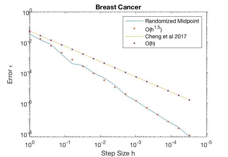
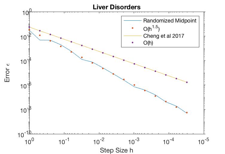
Figure 1: Error of random walks with different choice of step size.

In this section, we compare the algorithm from our paper, randomized midpoint method, with the one from [10]. We test the algorithms on the liver-disorders dataset and the breast-cancer dataset from UCL machine learning [17]. In both datasets, we observe a set of independent samples $\left\{x_{i},y_{i}\right\}_{i=1}^{m}$, where $y_{i}$ is the label, $x_{i}$ is the feature and $m$ is the number of samples. We sample from the target distribution $p^{*}(\theta)\propto\exp\left(-f(\theta)\right),$ where

$$f(\theta)=\frac{\lambda}{2}\left\|\theta\right\|^{2}+\frac{1}{m}\sum_{i=1}^{m}\log\left(\exp\left(-y_{i}x_{i}^{T}\theta\right)+1\right),$$

for regularization parameters $\lambda$. We set $\lambda$ to be $10^{-2}$ in our experiments. Figure 1 shows the error of randomized midpoint method and the algorithm from [10] with different step size $h$. The error is measured by the $\ell_{2}$ distance to the true solution of (3) at time $N=5000$, a time much greater than the mixing time of (3) for both datasets. Our results show that the $\epsilon$ dependence analysis of our algorithm and that of [10] are both tight. However, we note that the logistic function is infinitely differentiable, so there are methods of higher orders for this objective such as the standard midpoint method and Runge–Kutta methods.

Appendix A Brownian Motion Simulation

In this section, we introduce how $W_{1},$ $W_{2}$ and $W_{3}$ can be sampled. Let $\left\{B_{t}\right\}_{t\in[0,h]}$ be the standard $d$-dimensional Brownian motion on $t\in[0,h]$. In Algorithm $\text{\ref{al:lan}},$ $W_{1}=\int_{0}^{\alpha h}\left(1-e^{-2(\alpha h-s)}\right)\mathop{}\!\mathrm{d}B_{s}$, $W_{2}=\int_{0}^{h}\left(1-e^{-2(h-s)}\right)\mathop{}\!\mathrm{d}B_{s}$ and $W_{3}=\int_{0}^{h}e^{-2(h-s)}\mathop{}\!\mathrm{d}B_{s}.$ We define $G_{1}=\int_{0}^{\alpha h}e^{2s}\mathop{}\!\mathrm{d}B_{s}$, $G_{2}=\int_{\alpha h}^{h}e^{2s}\mathop{}\!\mathrm{d}B_{s}$, $H_{1}=\int_{0}^{\alpha h}\mathop{}\!\mathrm{d}B_{s}$ and $H_{2}=\int_{\alpha h}^{h}\mathop{}\!\mathrm{d}B_{s}$. Then, $W_{1}=H_{1}-e^{-2\alpha h}G_{1}$, $W_{2}=(H_{1}+H_{2})-e^{-2h}(G_{1}+G_{2})$ and $W_{3}=e^{-2h}(G_{1}+G_{2})$. It is sufficient to sample $H_{1}$, $H_{2}$, $G_{1}$ and $G_{2}$. We can show that $\left(G_{1},H_{1}\right)$ is independent of $\left(G_{2},H_{2}\right),$ and $\left(G_{1},H_{1}\right)$ and $\left(G_{2},H_{2}\right)$ both follow a $2d$-dimensional Gaussian distribution, which can be easily sampled.

Lemma 5.

Define $G_{1}=\int_{0}^{\alpha h}e^{2s}\mathop{}\!\mathrm{d}B_{s}$, $G_{2}=\int_{\alpha h}^{h}e^{2s}\mathop{}\!\mathrm{d}B_{s}$, $H_{1}=\int_{0}^{\alpha h}\mathop{}\!\mathrm{d}B_{s}$ and $H_{2}=\int_{\alpha h}^{h}\mathop{}\!\mathrm{d}B_{s}$. Then, $\left(G_{1},H_{1}\right)$ is independent of $\left(G_{2},H_{2}\right)$ . Moreover, $\left(G_{1},H_{1}\right)$ and $\left(G_{2},H_{2}\right)$ both follow a $2d$-dimensional Gaussian distribution with mean zero. Conditional on the choice of $\alpha$, their covariance is given by

$$\mathbb{E}\left[\left(G_{1}-\mathbb{E}G_{1}\right)\left(H_{1}-\mathbb{E}H_{1}\right)^{T}\right] = \frac{1}{2}\left(e^{2\alpha h}-1\right)\cdot I_{d},$$

$$\mathbb{E}\left[\left(G_{1}-\mathbb{E}G_{1}\right)\left(G_{1}-\mathbb{E}G_{1}\right)^{T}\right] = \frac{1}{4}\left(e^{4\alpha h}-1\right)\cdot I_{d},$$

$$\mathbb{E}\left[\left(H_{1}-\mathbb{E}H_{1}\right)\left(H_{1}-\mathbb{E}H_{1}\right)^{T}\right] = \alpha h\cdot I_{d},$$

$$\mathbb{E}\left[\left(G_{2}-\mathbb{E}G_{2}\right)\left(H_{2}-\mathbb{E}H_{2}\right)^{T}\right] = \frac{1}{2}\left(e^{2h}-e^{2\alpha h}\right)\cdot I_{d},$$

$$\mathbb{E}\left[\left(G_{2}-\mathbb{E}G_{2}\right)\left(G_{2}-\mathbb{E}G_{2}\right)^{T}\right] = \frac{1}{4}\left(e^{4h}-e^{4\alpha h}\right)\cdot I_{d},$$

$$\mathbb{E}\left[\left(H_{2}-\mathbb{E}H_{2}\right)\left(H_{2}-\mathbb{E}H_{2}\right)^{T}\right] = \left(h-\alpha h\right)\cdot I_{d}.$$

Proof.

By the definition of the standard Brownian motion, $\left(G_{1},H_{1}\right)$ is independent of $\left(G_{2},H_{2}\right)$ and $\left(G_{1},H_{1}\right)$ and $\left(G_{2},H_{2}\right)$ both have mean zero. Moreover,

$$\mathbb{E}\left[\left(G_{1}-\mathbb{E}G_{1}\right)\left(H_{1}-\mathbb{E}H_{1}\right)^{T}\right] =\mathbb{E}\left[\left(\int_{0}^{\alpha h}e^{2s}\mathop{}\!\mathrm{d}B_{s}\right)\left(\int_{0}^{\alpha h}\mathop{}\!\mathrm{d}B_{s}\right)^{T}\right]=\int_{0}^{\alpha h}e^{2s}\mathop{}\!\mathrm{d}s\cdot I_{d}$$

$$=\frac{1}{2}\left(e^{2\alpha h}-1\right)\cdot I_{d},$$

$$\mathbb{E}\left[\left(G_{1}-\mathbb{E}G_{1}\right)\left(G_{1}-\mathbb{E}G_{1}\right)^{T}\right] =\mathbb{E}\left[\left(\int_{0}^{\alpha h}e^{2s}\mathop{}\!\mathrm{d}B_{s}\right)\left(\int_{0}^{\alpha h}e^{2s}\mathop{}\!\mathrm{d}B_{s}\right)^{T}\right]=\int_{0}^{\alpha h}e^{4s}\mathop{}\!\mathrm{d}s\cdot I_{d}$$

$$=\frac{1}{4}\left(e^{4\alpha h}-1\right)\cdot I_{d},$$

and

$$\mathbb{E}\left[\left(H_{1}-\mathbb{E}H_{1}\right)\left(H_{1}-\mathbb{E}H_{1}\right)^{T}\right] = \alpha h\cdot I_{d}.$$

Similarly,

$$\mathbb{E}\left[\left(G_{2}-\mathbb{E}G_{2}\right)\left(H_{2}-\mathbb{E}H_{2}\right)^{T}\right] =\mathbb{E}\left[\left(\int_{\alpha h}^{h}e^{2s}\mathop{}\!\mathrm{d}B_{s}\right)\left(\int_{\alpha h}^{h}\mathop{}\!\mathrm{d}B_{s}\right)^{T}\right]=\int_{\alpha h}^{h}e^{2s}\mathop{}\!\mathrm{d}s\cdot I_{d}$$

$$=\frac{1}{2}\left(e^{2h}-e^{2\alpha h}\right)\cdot I_{d},$$

$$\mathbb{E}\left[\left(G_{1}-\mathbb{E}G_{1}\right)\left(G_{1}-\mathbb{E}G_{1}\right)^{T}\right] =\mathbb{E}\left[\left(\int_{\alpha h}^{h}e^{2s}\mathop{}\!\mathrm{d}B_{s}\right)\left(\int_{\alpha h}^{h}e^{2s}\mathop{}\!\mathrm{d}B_{s}\right)^{T}\right]=\int_{\alpha h}^{h}e^{4s}\mathop{}\!\mathrm{d}s\cdot I_{d}$$

$$=\frac{1}{4}\left(e^{4h}-e^{4\alpha h}\right)\cdot I_{d},$$

and

$$\mathbb{E}\left[\left(H_{2}-\mathbb{E}H_{2}\right)\left(H_{2}-\mathbb{E}H_{2}\right)^{T}\right] = \left(h-\alpha h\right)\cdot I_{d}.$$

∎

Appendix B Properties of the ULD and the Brownian motion

Here, we prove some properties of the ULD and the Brownian motion. These properties are used in Appendices C, D, E and F to prove the guarantee of our algorithm.

B.1 Properties of the ULD

Lemma 6.

Let $\left\{x(t)\right\}_{t\in[0,h]}$ and $\left\{v(t)\right\}_{t\in[0,h]}$ be the solution to the underdamped Langevin diffusion $\left(\ref{eq:ULD}\right)$ on $t\in[0,h]$. Assume that $h\leq\frac{1}{20}$ and $u=\frac{1}{L}$. We have the following bounds.

$$\mathbb{E}\sup_{t\in[0,h]}\left\|v(t)\right\|^{2} \leq O\left(\left\|v(0)\right\|^{2}+u^{2}h^{2}\left\|\nabla f(x(0))\right\|^{2}+udh\right),$$

$$\mathbb{E}\sup_{t\in[0,h]}\left\|\nabla f(x(t))\right\|^{2} \leq O\left(\left\|\nabla f(x(0))\right\|^{2}+L^{2}h^{2}\left\|v(0)\right\|^{2}+Ldh^{3}\right),$$

$$\mathbb{E}\sup_{t\in[0,h]}\left\|x(0)-x(t)\right\|^{2} \leq O\left(h^{2}\left\|v(0)\right\|^{2}+u^{2}h^{4}\left\|\nabla f(x(0))\right\|^{2}+udh^{3}\right)\text{,}$$

and

$$-\mathbb{E}\inf_{t\in[0,h]}\left\|v(t)\right\|^{2} \leq -\frac{1}{3}\left\|v(0)\right\|^{2}+O\left(u^{2}h^{2}\left\|\nabla f(x(0))\right\|^{2}+udh\right),$$

$$-\mathbb{E}\inf_{t\in[0,h]}\left\|\nabla f(x(t))\right\|^{2} \leq -\frac{1}{3}\left\|\nabla f(x(0))\right\|^{2}+O\left(h^{2}L^{2}\left\|v(0)\right\|^{2}+Ldh^{3}\right)\text{.}$$

Proof.

We first show the first three bounds. We can write $\mathbb{E}\sup_{t\in[0,h]}\left\|\nabla f(x(t))\right\|^{2}$ as

$$\mathbb{E}\sup_{t\in[0,h]}\left\|\nabla f(x(t))\right\|^{2}$$ (6)

$$\leq 2\left\|\nabla f(x(0))\right\|^{2}+2\mathbb{E}\sup_{t\in[0,h]}\left\|\nabla f(x(0))-\nabla f(x(t))\right\|^{2}$$

$$\leq 2\left\|\nabla f(x(0))\right\|^{2}+2L^{2}\mathbb{E}\sup_{t\in[0,h]}\left\|x(0)-x(t)\right\|^{2},$$

where the first step follows by Young’s inequality and the second step follows by $\nabla f$ is $L$-Lipschitz. To bound $\mathbb{E}\sup_{t\in[0,h]}\left\|x(0)-x(t)\right\|^{2}$,

$$\mathbb{E}\sup_{t\in[0,h]}\left\|x(0)-x(t)\right\|^{2} = \mathbb{E}\sup_{t\in[0,h]}\left\|\int_{0}^{t}v(s)\mathop{}\!\mathrm{d}s\right\|^{2}$$ (7)

$$\leq \mathbb{E}\sup_{t\in[0,h]}t\int_{0}^{t}\left\|v(s)\right\|^{2}\mathop{}\!\mathrm{d}s$$

$$\leq h^{2}\mathbb{E}\sup_{t\in[0,h]}\left\|v(t)\right\|^{2},$$

where the first step follows by the definition of $x$ and the second follows by the Cauchy-Schwarz inequality. To bound $\mathbb{E}\sup_{t\in[0,h]}\left\|v(t)\right\|^{2},$

$$\mathbb{E}\sup_{t\in[0,h]}\left\|v(t)\right\|^{2} = \mathbb{E}\sup_{t\in[0,h]}\left\|v(0)e^{-2t}-u\int_{0}^{t}e^{-2(t-s)}\nabla f(x(s))\mathop{}\!\mathrm{d}s+2\sqrt{u}\int_{0}^{t}e^{-2(t-s)}\mathop{}\!\mathrm{d}B_{s}\right\|^{2}$$ (8)

$$\leq 3\left\|v(0)\right\|^{2}+3u^{2}h^{2}\mathbb{E}\sup_{t\in[0,h]}\left\|\nabla f(x(t))\right\|^{2}+12u\mathbb{E}\sup_{t\in[0,h]}\left\|\int_{0}^{t}e^{-2(t-s)}\mathop{}\!\mathrm{d}B_{s}\right\|^{2}$$

$$\leq 3\left\|v(0)\right\|^{2}+3u^{2}h^{2}\mathbb{E}\sup_{t\in[0,h]}\left\|\nabla f(x(t))\right\|^{2}+60udh,$$

where the first step follows by the definition of ULD, the second step follows by the inequality $(a+b+c)^{2}\leq 3a^{2}+3b^{2}+3c^{2}$ and the third step follows by Lemma $\text{\ref{lem:Brownian}}.$ Then, combining $\left(\ref{eq:ideal_1}\right)$, $\left(\text{\ref{eq:ideal_2}}\right)$ and $\left(\text{\ref{eq:ideal_3}}\right)$, we have

$$\mathbb{E}\sup_{t\in[0,h]}\left\|\nabla f(x(t))\right\|^{2} \leq 2\left\|\nabla f(x(0))\right\|^{2}+2L^{2}\mathbb{E}\sup_{t\in[0,h]}\left\|x(0)-x(t)\right\|^{2}$$

$$\leq 2\left\|\nabla f(x(0))\right\|^{2}+2L^{2}h^{2}\mathbb{E}\sup_{t\in[0,h]}\left\|v(t)\right\|^{2}$$

$$\leq 2\left\|\nabla f(x(0))\right\|^{2}+6h^{4}\mathbb{E}\sup_{t\in[0,h]}\left\|\nabla f(x(t))\right\|^{2}+6L^{2}h^{2}\left\|v(0)\right\|^{2}+120Ldh^{3}.$$

Since $6h^{4}\leq\frac{1}{4}$,

$$\mathbb{E}\sup_{t\in[0,h]}\left\|\nabla f(x(t))\right\|^{2} \leq 3\left\|\nabla f(x(0))\right\|^{2}+8L^{2}h^{2}\left\|v(0)\right\|^{2}+160Ldh^{3}$$ (9)

$$\leq O\left(\left\|\nabla f(x(0))\right\|^{2}+L^{2}h^{2}\left\|v(0)\right\|^{2}+Ldh^{3}\right).$$

By $\left(\ref{eq:ideal_3}\right)$ and $\left(\ref{eq:ideal_4}\right)$,

$$\mathbb{E}\sup_{t\in[0,h]}\left\|v(t)\right\|^{2} \leq 3\left\|v(0)\right\|^{2}+3u^{2}h^{2}\mathbb{E}\sup_{t\in[0,h]}\left\|\nabla f(x(t))\right\|^{2}+60udh$$

$$\leq 3\left\|v(0)\right\|^{2}+3u^{2}h^{2}\cdot O\left(\left\|\nabla f(x(0))\right\|^{2}+L^{2}h^{2}\left\|v(0)\right\|^{2}+Ldh^{3}\right)+60udh$$

$$\leq O\left(\left\|v(0)\right\|^{2}+u^{2}h^{2}\left\|\nabla f(x(0))\right\|^{2}+udh\right).$$

where the last step follows by $h$ is small.

By $\left(\text{\ref{eq:ideal_2}}\right)$ and $\left(\text{\ref{eq:ideal_4}}\right)$,

$$\mathbb{E}\sup_{t\in[0,h]}\left\|x(0)-x(t)\right\|^{2} \leq h^{2}\mathbb{E}\sup_{t\in[0,h]}\left\|v(t)\right\|^{2}$$ (10)

$$\leq O\left(h^{2}\left\|v(0)\right\|^{2}+u^{2}h^{4}\left\|\nabla f(x(0))\right\|^{2}+udh^{3}\right).$$

To prove the fourth claim,

$$\inf_{t\in[0,h]}\left\|v(t)\right\|^{2}$$

$$= \inf_{t\in[0,h]}\left\|v(0)e^{-2t}-u\int_{0}^{t}e^{-2(t-s)}\nabla f(x(s))\mathop{}\!\mathrm{d}s+2\sqrt{u}\int_{0}^{t}e^{-2(t-s)}\mathop{}\!\mathrm{d}B_{s}\right\|^{2}$$

$$\geq \inf_{t\in[0,h]}\Bigg{[}e^{-4t}\left\|v(0)\right\|^{2}-2e^{-2t}v(0)^{T}\left(u\int_{0}^{t}e^{-2(t-s)}\nabla f(x(s))\mathop{}\!\mathrm{d}s\right)$$

$$+2e^{-2t}v(0)^{T}\left(2\sqrt{u}\int_{0}^{t}e^{-2(t-s)}\mathop{}\!\mathrm{d}B_{s}\right)\Bigg{]}$$

$$\geq \inf_{t\in[0,h]}\Bigg{[}e^{-4t}\left\|v(0)\right\|^{2}-\frac{1}{2}e^{-4t}\left\|v(0)\right\|^{2}-4\left\|u\int_{0}^{t}e^{-2(t-s)}\nabla f(x(s))\mathop{}\!\mathrm{d}s\right\|^{2}$$

$$-4\left\|2\sqrt{u}\int_{0}^{t}e^{-2(t-s)}\mathop{}\!\mathrm{d}B_{s}\right\|^{2}\Bigg{]}$$

$$\geq \inf_{t\in[0,h]}\left[\frac{1}{2}(1-4h)\left\|v(0)\right\|^{2}-4u^{2}h^{2}\sup_{s\in[0,t]}\left\|\nabla f(x(s))\right\|^{2}-16u\left\|\int_{0}^{t}e^{-2(t-s)}\mathop{}\!\mathrm{d}B_{s}\right\|^{2}\right]$$

$$\geq \frac{1}{2}(1-4h)\left\|v(0)\right\|^{2}-4u^{2}h^{2}\sup_{t\in[0,h]}\left\|\nabla f(x(t))\right\|^{2}-16u\sup_{t\in[0,h]}\left\|\int_{0}^{t}e^{-2(t-s)}\mathop{}\!\mathrm{d}B_{s}\right\|^{2},$$

where the first step follows by the definition of $v$ , the second step follows by the inequality $(a+b+c)^{2}\geq a^{2}+2a(b+c)$, the third step follows by the inequality $2ab\leq a^{2}+b^{2}$ , the fourth step follows by $e^{-4t}\geq 1-4t$, and the last step follows by $h$ is small.

Then, by $\left(\ref{eq:ideal_4}\right)$ and Lemma $\text{\ref{lem:Brownian}},$

$$-\mathbb{E}\inf_{t\in[0,h]}\left\|v(t)\right\|^{2} \leq -\frac{1}{3}\left\|v(0)\right\|^{2}+O\left(u^{2}h^{2}\left\|\nabla f(x(0))\right\|^{2}+udh\right).$$

To show the lower bound on $\mathbb{E}\inf_{t\in[0,h]}\left\|\nabla f(x(t))\right\|^{2}$, notice that

$$\mathbb{E}\inf_{t\in[0,h]}\left\|\nabla f(x(t))\right\|^{2} \geq \frac{1}{2}\left\|\nabla f(x(0))\right\|^{2}-\mathbb{E}\sup_{t\in[0,h]}\left\|\nabla f(x(t))-\nabla f(x(0))\right\|^{2}$$

$$\geq \frac{1}{2}\left\|\nabla f(x(0))\right\|^{2}-L^{2}\mathbb{E}\sup_{t\in[0,h]}\left\|x(t)-x(0)\right\|^{2}.$$

Then, by$\left(\ref{eq:ideal_5}\right)$ and $h\leq\frac{1}{20}$,

$$-\mathbb{E}\inf_{t\in[0,h]}\left\|\nabla f(x(t))\right\| \leq -\frac{1}{3}\left\|\nabla f(x(0))\right\|^{2}+O\left(h^{2}L^{2}\left\|v(0)\right\|^{2}+Ldh^{3}\right)\text{.}$$

∎

B.2 Properties of the Brownian Motion

Lemma 7 (Doob’s maximal inequality [16]).

Suppose $\{X(t):t\geq 0\}$ is a continuous martingale. Then, for any $t\geq 0$,

$$\mathbb{E}\left[\sup_{0\leq s\leq t}\left|X(s)\right|^{2}\right] \leq 4\mathbb{E}\left[\left|X(t)\right|^{2}\right].$$

Using the Doob’s maximal inequality, we can show the following lemma.

Lemma 8.

For $d$-dimensional Brownian motion $B_{t}$ on $t\in[0,h]$, assuming $h\leq\frac{1}{10},$

$$\mathbb{E}\left[\sup_{0\leq t\leq h}\left\|B(t)\right\|^{2}\right]\leq 4dh,\text{ and }\mathbb{E}\left[\sup_{0\leq t\leq h}\left\|\int_{0}^{t}e^{-2(t-s)}dB_{s}\right\|^{2}\right]\leq 5dh.$$

Proof.

To show the first inequality,

$$\mathbb{E}\left[\sup_{0\leq t\leq h}\left\|B(t)\right\|^{2}\right] \leq \sum_{i=1}^{d}\mathbb{E}\left[\sup_{0\leq t\leq h}\left|B_{i}(t)\right|^{2}\right]$$

$$\leq 4d\mathbb{E}\left[\left|B_{i}(h)\right|^{2}\right]$$

$$= 4dh,$$

where the second step follows by Lemma 7. To show the second inequality,

$$\mathbb{E}\left[\sup_{0\leq t\leq h}\left\|\int_{0}^{t}e^{-2(t-s)}dB_{s}\right\|^{2}\right] \leq \mathbb{E}\left[\sup_{0\leq t\leq h}e^{-4t}\left\|\int_{0}^{t}e^{2s}dB_{s}\right\|^{2}\right]$$

$$\leq \mathbb{E}\left[\sup_{0\leq t\leq h}\left\|\int_{0}^{t}e^{2s}dB_{s}\right\|^{2}\right]$$

$$\leq \sum_{i=1}^{d}\mathbb{E}\left[\sup_{0\leq t\leq h}\left|\int_{0}^{t}e^{2s}dB_{s,i}\right|^{2}\right]$$

$$\leq 4\sum_{i=1}^{d}\mathbb{E}\left[\left|\int_{0}^{h}e^{2s}dB_{s,i}\right|^{2}\right]$$

$$= 4\sum_{i=1}^{d}\int_{0}^{h}e^{4s}ds$$

$$\leq 5dh,$$

where the second step follows by $e^{-4t}\leq 1$, the fourth step follows by Lemma 7 and the last inequality follows by $\int_{0}^{h}e^{4s}ds\leq\frac{5}{4}h$ for $h\leq\frac{1}{10}.$ ∎

Appendix C Discretization Error of Algorithm 1

In this section, we bound the discretization error of Algorithm 1 in each iteration. In order to prove Lemma 2, we first prove Lemma 9, stated next.

Lemma 9.

Let $\alpha$ be the random number chosen in iteration $n$. Let $x_{n+\frac{1}{2}}$ be the intermediate value computed in iteration $n$ of Algorithm 1. Let $\left\{x_{n}^{*}(t)\right\}_{t\in[0,h]}$ be the ideal underdamped Langevin diffusion starting from $x_{n}^{*}(0)=x_{n}$ coupled through a shared Brownian motion with $x_{n+\frac{1}{2}}.$ Assume that $h\leq\frac{1}{20}$. Then,

$$\mathbb{E}\left\|\nabla f(x_{n+\frac{1}{2}})-\nabla f(x_{n}^{*}(\alpha h))\right\|^{2} \leq O\left(h^{6}L^{2}\left\|v_{n}\right\|^{2}+h^{8}\left\|\nabla f(x_{n})\right\|^{2}+Ldh^{7}\right).$$

Proof.

We have the bound

$$\mathbb{E}\left\|\nabla f(x_{n+\frac{1}{2}})-\nabla f(x_{n}^{*}(\alpha h))\right\|^{2}$$

$$\leq L^{2}\mathbb{E}\left\|x_{n+\frac{1}{2}}-x_{n}^{*}(\alpha h)\right\|^{2}$$

$$= L^{2}\mathbb{E}\left\|\frac{1}{2}u\int_{0}^{\alpha h}\left(1-e^{-2(\alpha h-s)}\right)\left(\nabla f(x_{n}^{*}(0))-\nabla f(x_{n}^{*}(s))\right)\mathop{}\!\mathrm{d}s\right\|^{2}$$

$$\leq \frac{1}{4}\mathbb{E}\left[\int_{0}^{\alpha h}\left(1-e^{-2(\alpha h-s)}\right)^{2}\mathop{}\!\mathrm{d}s\cdot\alpha h\cdot\left(\sup_{t\in[0,h]}\left\|\nabla f(x_{n}^{*}(0))-\nabla f(x_{n}^{*}(t))\right\|^{2}\right)\right]$$

$$\leq h^{4}\mathbb{E}\sup_{t\in[0,h]}\left\|\nabla f(x_{n}^{*}(0))-\nabla f(x_{n}^{*}(t))\right\|^{2}$$

$$\leq L^{2}h^{4}\mathbb{E}\sup_{t\in[0,h]}\left\|x_{n}^{*}(0)-x_{n}^{*}(t)\right\|^{2}$$

$$\leq O\left(h^{6}L^{2}\left\|v_{n}\right\|^{2}+h^{8}\left\|\nabla f(x_{n})\right\|^{2}+Ldh^{7}\right),$$

where the first and the fifth step follows by $\nabla f$ is $L$-Lipschitz, the third step follows by Cauchy-Schwarz inequality, the fourth step follows by $1-e^{-2(\alpha h-t)}\leq 2h$ and the last step follows by Lemma 6. ∎

Now, we are ready to prove Lemma 2.

Proof.

To show the first claim,

$$\left\|\mathbb{E}_{\alpha}x_{n+1}-x_{n}^{*}(h)\right\|^{2}$$

$$= \left\|\mathbb{E}_{\alpha}\frac{1}{2}uh\left(1-e^{-2(h-\alpha h)}\right)\nabla f(x_{n+\frac{1}{2}})-\frac{1}{2}u\int_{0}^{h}\left(1-e^{-2(h-s)}\right)\nabla f(x_{n}^{*}(s))\mathop{}\!\mathrm{d}s\right\|^{2}$$

$$\leq \frac{1}{2}\mathbb{E}_{\alpha}\left\|uh\left(1-e^{-2(h-\alpha h)}\right)\nabla f(x_{n+\frac{1}{2}})-uh\left(1-e^{-2(h-\alpha h)}\right)\nabla f(x_{n}^{*}(\alpha h))\right\|^{2}$$

$$+\frac{1}{2}\left\|\mathbb{E}_{\alpha}uh\left(1-e^{-2(h-\alpha h)}\right)\nabla f(x_{n}^{*}(\alpha h))-u\int_{0}^{h}\left(1-e^{-2(h-s)}\right)\nabla f(x_{n}^{*}(s))\mathop{}\!\mathrm{d}s\right\|^{2}$$

$$\leq \frac{1}{2}u^{2}h^{2}\mathbb{E}_{\alpha}\left[\left(1-e^{-2(h-\alpha h)}\right)^{2}\left\|\nabla f(x_{n+\frac{1}{2}})-\nabla f(x_{n}^{*}(\alpha h))\right\|^{2}\right]+0$$

$$\leq 2u^{2}h^{4}\mathbb{E}_{\alpha}\left\|\nabla f(x_{n+\frac{1}{2}})-\nabla f(x_{n}^{*}(\alpha h))\right\|^{2},$$

where the first step follows by the definition of $x_{n+1}$, the second step follows by Young’s inequality, the third step follows by

$$\mathbb{E}_{\alpha}h\left(1-e^{-2(h-\alpha h)}\right)\nabla f(x_{n}^{*}(\alpha h))=\int_{0}^{h}\left(1-e^{-2(h-s)}\right)\nabla f(x_{n}^{*}(s))\mathop{}\!\mathrm{d}s,$$

and the fourth step follows by $1-e^{-2(h-\alpha h)}\leq 2h$ . By Lemma 9,

$$\mathbb{E}\left\|\mathbb{E}_{\alpha}x_{n+1}-x_{n}^{*}(h)\right\|^{2} \leq O\left(h^{10}\left\|v_{n}\right\|^{2}+u^{2}h^{12}\left\|\nabla f(x_{n})\right\|^{2}+udh^{11}\right).$$

To show the second claim,

$$\mathbb{E}\left\|x_{n+1}-x_{n}^{*}(h)\right\|^{2}$$

$$\leq \frac{3}{4}\mathbb{E}\left\|uh\left(1-e^{-2(h-\alpha h)}\right)\nabla f(x_{n+\frac{1}{2}})-uh\left(1-e^{-2(h-\alpha h)}\right)\nabla f(x_{n}^{*}(\alpha h))\right\|^{2}$$

$$+\frac{3}{4}\mathbb{E}\left\|uh\left(1-e^{-2(h-\alpha h)}\right)\nabla f(x_{n}^{*}(\alpha h))-u\int_{0}^{h}\left(1-e^{-2(h-\alpha h)}\right)\nabla f(x_{n}^{*}(s))\mathop{}\!\mathrm{d}s\right\|^{2}$$

$$+\frac{3}{4}\mathbb{E}\left\|u\int_{0}^{h}\left(1-e^{-2(h-\alpha h)}\right)\nabla f(x_{n}^{*}(s))\mathop{}\!\mathrm{d}s-u\int_{0}^{h}\left(1-e^{-2(h-s)}\right)\nabla f(x_{n}^{*}(s))\mathop{}\!\mathrm{d}s\right\|^{2},$$

which follows by definition and Young’s inequality. To bound the second term,

$$\left\|uh\left(1-e^{-2(h-\alpha h)}\right)\nabla f(x_{n}^{*}(\alpha h))-u\int_{0}^{h}\left(1-e^{-2(h-\alpha h)}\right)\nabla f(x_{n}^{*}(s))\mathop{}\!\mathrm{d}s\right\|^{2}$$ (11)

$$= \left\|u\int_{0}^{h}\left(1-e^{-2(h-\alpha h)}\right)\left(\nabla f(x_{n}^{*}(\alpha h))-\nabla f(x_{n}^{*}(s))\right)\mathop{}\!\mathrm{d}s\right\|^{2}$$

$$\leq u^{2}\int_{0}^{h}\left(1-e^{-2(h-\alpha h)}\right)^{2}\mathop{}\!\mathrm{d}s\cdot\sup_{t\in[0,h]}\left\|\nabla f(x_{n}^{*}(\alpha h))-\nabla f(x_{n}^{*}(t))\right\|^{2}\cdot h$$

$$\leq 4u^{2}h^{4}\sup_{t\in[0,h]}\left\|\nabla f(x_{n}^{*}(\alpha h))-\nabla f(x_{n}^{*}(t))\right\|^{2}$$

$$\leq 16h^{4}\sup_{t\in[0,h]}\left\|x_{n}^{*}(0)-x_{n}^{*}(t)\right\|^{2}$$

where the second step follows by the Cauchy-Schwarz inequality. The third term satisfies

$$\left\|u\int_{0}^{h}\left(1-e^{-2(h-\alpha h)}\right)\nabla f(x_{n}^{*}(s))\mathop{}\!\mathrm{d}s-u\int_{0}^{h}\left(1-e^{-2(h-s)}\right)\nabla f(x_{n}^{*}(s))\mathop{}\!\mathrm{d}s\right\|^{2}$$ (12)

$$= u^{2}\left\|\int_{0}^{h}\left(e^{-2(h-s)}-e^{-2(h-\alpha h)}\right)\nabla f(x_{n}^{*}(s))\mathop{}\!\mathrm{d}s\right\|^{2}$$

$$\leq 4u^{2}h^{4}\sup_{t\in[0,h]}\left\|\nabla f(x_{n}^{*}(t))\right\|^{2},$$

where the second step follows by the Cauchy Schwarz inequality and $\left|e^{-2(h-s)}-e^{-2(h-\alpha h)}\right|\leq 2h$. Thus,

$$\mathbb{E}\left\|x_{n+1}-x_{n}^{*}(h)\right\|^{2}$$

$$\leq 3u^{2}h^{4}\mathbb{E}\left\|\nabla f(x_{n+\frac{1}{2}})-\nabla f(x_{n}^{*}(\alpha h))\right\|^{2}+12h^{4}\mathbb{E}\sup_{t\in[0,h]}\left\|x_{n}^{*}(0)-x_{n}^{*}(t)\right\|^{2}$$

$$+3u^{2}h^{4}\mathbb{E}\sup_{t\in[0,h]}\left\|\nabla f(x_{n}^{*}(t))\right\|^{2}$$

$$\leq 3h^{4}\cdot O\left(h^{6}\left\|v_{n}\right\|^{2}+h^{8}u^{2}\left\|\nabla f(x_{n})\right\|^{2}+udh^{7}\right)$$

$$+12h^{4}\cdot O\left(h^{2}\left\|v_{n}\right\|^{2}+u^{2}h^{4}\left\|\nabla f(x_{n})\right\|^{2}+udh^{3}\right)$$

$$+3u^{2}h^{4}\cdot O\left(\left\|\nabla f(x_{n})\right\|^{2}+L^{2}h^{2}\left\|v_{n}\right\|^{2}+Mdh^{3}\right)$$

$$\leq O\left(h^{6}\left\|v_{n}\right\|^{2}+u^{2}h^{4}\left\|\nabla f(x_{n})\right\|^{2}+udh^{7}\right).$$

where the first step follows by $\left(\text{\ref{eq:error_1}}\right)$ and $\left(\text{\ref{eq:error_2}}\right)$, the second step follows by Lemma 6 and Lemma 9, and the last inequality follows by $h\leq 1$.

To show the third claim,

$$\mathbb{E}\left\|\mathbb{E}_{\alpha}v_{n+1}-v_{n}^{*}(h)\right\|^{2} = \mathbb{E}\left\|\mathbb{E}_{\alpha}uhe^{-2(h-\alpha h)}\nabla f(x_{n+\frac{1}{2}})-u\int_{0}^{h}e^{-2(h-s)}\nabla f(x_{n}^{*}(s))\mathop{}\!\mathrm{d}s\right\|^{2}$$

$$\leq 2\mathbb{E}\left\|uhe^{-2(h-\alpha h)}\nabla f(x_{n+\frac{1}{2}})-uhe^{-2(h-\alpha h)}\nabla f(x_{n}^{*}(\alpha h))\right\|^{2}$$

$$+2\mathbb{E}\left\|\mathbb{E}_{\alpha}uhe^{-2(h-\alpha h)}\nabla f(x_{n}^{*}(\alpha h))-u\int_{0}^{h}e^{-2(h-s)}\nabla f(x_{n}^{*}(s))\mathop{}\!\mathrm{d}s\right\|^{2}$$

$$\leq 2u^{2}h^{2}\mathbb{E}\left\|\nabla f(x_{n+\frac{1}{2}})-\nabla f(x_{n}^{*}(\alpha h))\right\|^{2}+0$$

$$\leq O\left(h^{8}\left\|v_{n}\right\|^{2}+u^{2}h^{10}\left\|\nabla f(x_{n})\right\|^{2}+udh^{9}\right),$$

where the first step follows by Young’s inequality, the second step follows by

$$\mathbb{E}_{\alpha}uhe^{-2(h-\alpha h)}\nabla f(x_{n}^{*}(\alpha h)) = u\int_{0}^{h}e^{-2(h-t)}\nabla f(x_{n}^{*}(t))\mathop{}\!\mathrm{d}t,$$

and $e^{-2(h-\alpha h)}\leq 1$, and the third step follows by Lemma $\text{\ref{lem:grad_f}}.$

To show the last claim,

$$\mathbb{E}\left\|v_{n+1}-v_{n}^{*}(h)\right\|^{2}$$

$$= \mathbb{E}\left\|uhe^{-2(h-\alpha h)}\nabla f(x_{n+\frac{1}{2}})-u\int_{0}^{h}e^{-2(h-s)}\nabla f(x^{*}(s))\mathop{}\!\mathrm{d}s\right\|^{2}$$

$$\leq 3\mathbb{E}\left\|uhe^{-2(h-\alpha h)}\nabla f(x_{n+\frac{1}{2}})-uhe^{-2(h-\alpha h)}\nabla f(x^{*}(\alpha h))\right\|^{2}$$

$$+3\mathbb{E}\left\|u\int_{0}^{h}e^{-2(h-\alpha h)}\nabla f(x_{n}^{*}(\alpha h))\mathop{}\!\mathrm{d}t-u\int_{0}^{h}e^{-2(h-\alpha h)}\nabla f(x_{n}^{*}(s))\mathop{}\!\mathrm{d}s\right\|^{2}$$

$$+3\mathbb{E}\left\|u\int_{0}^{h}e^{-2(h-\alpha h)}\nabla f(x_{n}^{*}(s))\mathop{}\!\mathrm{d}s-u\int_{0}^{h}e^{-2(h-s)}\nabla f(x_{n}^{*}(s))\mathop{}\!\mathrm{d}s\right\|^{2}$$

$$\leq 3u^{2}h^{2}\mathbb{E}\left\|\nabla f(x_{n+\frac{1}{2}})-\nabla f(x_{n}^{*}(\alpha h))\right\|^{2}+3h^{2}\mathbb{E}\sup_{t\in[0,h]}\left\|x_{n}^{*}(\alpha h)-x_{n}^{*}(t)\right\|^{2}$$

$$+12u^{2}h^{4}\mathbb{E}\sup_{t\in[0,h]}\left\|\nabla f(x_{n}^{*}(t))\right\|^{2}$$

$$\leq 3u^{2}h^{2}\cdot O\left(h^{6}L^{2}\left\|v_{n}\right\|^{2}+h^{8}\left\|\nabla f(x_{n})\right\|^{2}+Ldh^{7}\right)$$

$$+3h^{2}\cdot O\left(h^{2}\left\|v_{n}\right\|^{2}+u^{2}h^{4}\left\|\nabla f(x_{n})\right\|^{2}+udh^{3}\right)$$

$$+12u^{2}h^{4}\cdot O\left(\left\|\nabla f(x_{n})\right\|^{2}+L^{2}h^{2}\left\|v_{n}\right\|^{2}+Ldh^{3}\right)$$

$$\leq O\left(h^{4}\left\|v_{n}\right\|^{2}+u^{2}h^{4}\left\|\nabla f(x_{n})\right\|^{2}+udh^{5}\right),$$

where the first step follows by the definition, the second step follows by Young’s inequality, the third follows by $e^{-2(h-\alpha h)}-e^{-2(h-s)}\leq 2h$ , the fourth step follows by Lemma 9 and Lemma 6 and the last inequality follows by $h\leq 1.$ ∎

Appendix D Bounds on $\left\|\nabla f(x)\right\|$ and $\left\|v\right\|$

In this section, we bound the sum of $\left\|\nabla f(x_{n})\right\|^{2}$ and $\left\|v_{n}\right\|^{2}$ over all iterations $n$, $\sum_{n=0}^{N-1}\mathbb{E}\left\|\nabla f(x_{n})\right\|^{2}$ and $\sum_{n=0}^{N-1}\mathbb{E}\left\|v_{n}\right\|^{2}$. In Appendix E, we use the results in this appendix together with Lemma 2 to prove the guarantee of our algorithm.

Lemma 10.

Assume $h\leq\frac{1}{20}$. For each iteration $n$, let $x_{n}$ be the starting point of iteration $n$ of Algorithm 1. Let $\left\{v_{n}(t),x_{n}(t)\right\}_{t\in[0,h]}$ be the solution of the exact underdamped Langevin diffusion starting from $\left(v_{n},x_{n}\right)$ . Let $\mathbb{E}_{\alpha}$ be the expectation over the random choice of $\alpha$ in iteration $n$. Then, the difference between the value of $f$ on the starting point of iteration $n+1$, $x_{n+1}$, and that of $x_{n}(h)$ satisfies

$$\mathbb{E}f(x_{n+1}(0))-f(x_{n}(h)) \leq O\left(uh^{3}\left\|\nabla f(x_{n}(0))\right\|^{2}+Lh^{5}\left\|v_{n}(0)\right\|^{2}+dh^{6}\right).$$

Proof.

We first consider the expectation over the choice of $\alpha$ in iteration $n$,

$$\mathbb{E}_{\alpha}f(x_{n+1}(0))$$

$$\leq f(x_{n}(h))+\nabla f(x_{n}(h))^{T}\left(\mathbb{E}_{\alpha}x_{n+1}(0)-x_{n}(h)\right)+\frac{L}{2}\mathbb{E}_{\alpha}\left\|x_{n+1}(0)-x_{n}(h)\right\|^{2}$$

$$\leq f(x_{n}(h))+\left\|\nabla f(x_{n}(h))\right\|\left\|\mathbb{E}_{\alpha}x_{n+1}(0)-x_{n}(h)\right\|+\frac{L}{2}\mathbb{E}_{\alpha}\left\|x_{n+1}(0)-x_{n}(h)\right\|^{2}$$

$$\leq f(x_{n}(h))+uh^{3}\left\|\nabla f(x_{n}(h))\right\|^{2}+\frac{L}{h^{3}}\left\|\mathbb{E}_{\alpha}x_{n+1}(0)-x_{n}(h)\right\|^{2}+\frac{L}{2}\mathbb{E}_{\alpha}\left\|x_{n+1}(0)-x_{n}(h)\right\|^{2},$$

where the first step follows by $\nabla f$ is $L$-Lipschitz, the second step follows by Cauchy-Schwarz inequality and the third step follows by Young’s inequality. By Lemma 2 and Lemma $\text{\ref{lem:idealULD}},$

$$\mathbb{E}f(x_{n+1}(0)) \leq \mathbb{E}f(x_{n}(h))+uh^{3}\mathbb{E}\left\|\nabla f(x_{n}(h))\right\|^{2}+\frac{L}{h^{3}}\mathbb{E}\left\|\mathbb{E}_{\alpha}x_{n+1}(0)-x_{n}(h)\right\|^{2}$$

$$+\frac{L}{2}\mathbb{E}\left\|x_{n+1}(0)-x_{n}(h)\right\|^{2}$$

$$\leq \mathbb{E}f(x_{n}(h))+\mathbb{E}uh^{3}\cdot O\left(\left\|\nabla f(x_{n}(0))\right\|^{2}+L^{2}h^{2}\left\|v_{n}(0)\right\|^{2}+Ldh^{3}\right)$$

$$+\mathbb{E}\frac{L}{h^{3}}\cdot O\left(h^{10}\left\|v_{n}(0)\right\|^{2}+u^{2}h^{12}\left\|\nabla f(x_{n}(0))\right\|^{2}+udh^{11}\right)$$

$$+\mathbb{E}\frac{L}{2}\cdot O\left(h^{6}\left\|v_{n}(0)\right\|^{2}+h^{4}u^{2}\left\|\nabla f(x_{n}(0))\right\|^{2}+udh^{7}\right)$$

$$\leq \mathbb{E}f(x_{n}(h))+O\left(uh^{3}\mathbb{E}\left\|\nabla f(x_{n}(0))\right\|^{2}+Lh^{5}\mathbb{E}\left\|v_{n}(0)\right\|^{2}+dh^{6}\right).$$

where the second step follows by Lemma 2 and Lemma 6, and the last step follows by $h\leq\frac{1}{20}$. ∎

Lemma 11.

Assume $h$ is smaller than some given constant. For each iteration $n=0,...,N-1$, let $\left(v_{n},x_{n}\right)$ be the starting point of Algorithm 1 in iteration $n$. Then,

$$\sum_{n=0}^{N-1}\mathbb{E}\left\|v_{n}\right\|^{2} \leq O\left(u^{2}h\sum_{n=0}^{N-1}\mathbb{E}\left\|\nabla f(x_{n})\right\|^{2}+Nud\right).$$

Proof.

Let $\left\{v_{n}(t),x_{n}(t)\right\}_{t\in[0,h]}$ be the solution of the exact underdamped Langevin diffusion starting from $\left(v_{n},x_{n}\right)$ . By definition, for $t\in[0,h]$,

$$\frac{\mathop{}\!\mathrm{d}f(x_{n}(t))}{\mathop{}\!\mathrm{d}t} = \nabla f(x_{n}(t))^{T}\frac{\mathop{}\!\mathrm{d}x_{n}(t)}{\mathop{}\!\mathrm{d}t}$$

$$= \nabla f(x_{n}(t))^{T}v_{n}(t),$$

so

$$f(x_{n}(h)) = f(x_{n}(0))+\int_{0}^{h}\mathop{}\!\mathrm{d}f(x_{n}(t))$$ (13)

$$= f(x_{n}(0))+\int_{0}^{h}\nabla f(x_{n}(t))^{T}v_{n}(t)\mathop{}\!\mathrm{d}t.$$

Also, since

$$\mathop{}\!\mathrm{d}v_{n}(t) = \left(-2v_{n}(t)-u\nabla f(x_{n}(t))\right)\mathop{}\!\mathrm{d}t+2\sqrt{u}\mathop{}\!\mathrm{d}B_{t},$$

by Ito’s lemma,

$$\mathop{}\!\mathrm{d}\frac{1}{2}\left\|v_{n}(t)\right\|^{2} = \left\langle v_{n}(t),2\sqrt{u}\mathop{}\!\mathrm{d}B_{t}\right\rangle+\left(\left\langle v_{n}(t),-2v_{n}(t)-u\nabla f(x_{n}(t))\right\rangle+\frac{1}{2}\cdot 4u\text{Tr}(I_{d})\right)\mathop{}\!\mathrm{d}t$$

$$= 2\sqrt{u}v_{n}(t)^{T}\mathop{}\!\mathrm{d}B_{t}+\left(-2\left\|v_{n}(t)\right\|^{2}-uv_{n}(t)^{T}\nabla f(x_{n}(t))+2ud\right)\mathop{}\!\mathrm{d}t,$$

and therefore

$$\mathbb{E}\frac{1}{2u}\left\|v_{n}(h)\right\|^{2}=\mathbb{E}\frac{1}{2u}\left\|v_{n}(0)\right\|^{2}+\mathbb{E}\int_{0}^{h}\left(4d-\frac{2}{u}\left\|v_{n}(t)\right\|^{2}-v_{n}(t)^{T}\nabla f(x_{n}(t))+2d\right)\mathop{}\!\mathrm{d}t.$$ (14)

Now, we consider the term $\frac{1}{2u}\left\|v_{n}(h)\right\|^{2}+f(x_{n}(h)).$ By $\left(\ref{eq:sum_v_2}\right)$and $\left(\ref{eq:sum_v_1}\right)$,

$$\mathbb{E}\left[\frac{1}{2u}\left\|v_{n}(h)\right\|^{2}+f(x_{n}(h))\right]$$

$$= \mathbb{E}\left[\frac{1}{2u}\left\|v_{n}(0)\right\|^{2}+f(x_{n}(0))+\int_{0}^{h}\left(-\frac{2}{u}\left\|v_{n}(t)\right\|^{2}+6d\right)\mathop{}\!\mathrm{d}t\right]$$

$$\leq \mathbb{E}\left[\frac{1}{2u}\left\|v_{n}(0)\right\|^{2}+f(x_{n}(0))-\frac{2}{u}h\inf_{t\in[0,h]}\left\|v_{n}(t)\right\|^{2}+6dh\right]$$

$$\leq \mathbb{E}\left[\frac{1}{2u}\left\|v_{n}(0)\right\|^{2}+f(x_{n}(0))\right]-\frac{2}{3}hL\mathbb{E}\left\|v_{n}(0)\right\|^{2}+O\left(uh^{3}\mathbb{E}\left\|\nabla f(x_{n}(0))\right\|^{2}+dh\right),$$

where the first step follows by $\left(\ref{eq:sum_v_2}\right)$ and $\left(\ref{eq:sum_v_1}\right)$ and the third step follows by Lemma 6.

Since

$$\mathbb{E}\left[\left\|v_{n+1}(0)\right\|^{2}-\left\|v_{n}(h)\right\|^{2}\right]$$

$$= \mathbb{E}\left(v_{n+1}(0)-v_{n}(h)\right)^{T}\left(v_{n+1}(0)+v_{n}(h)\right)$$

$$\leq \frac{1}{h^{2}}\mathbb{E}\left\|v_{n+1}(0)-v_{n}(h)\right\|^{2}+\frac{1}{2}h^{2}\mathbb{E}\left\|v_{n+1}(0)+v_{n}(h)\right\|^{2}$$

$$\leq \frac{1}{h^{2}}\mathbb{E}\left\|v_{n+1}(0)-v_{n}(h)\right\|^{2}+h^{2}\mathbb{E}\left\|v_{n+1}(0)-v_{n}(h)\right\|^{2}+4h^{2}\mathbb{E}\left\|v_{n}(h)\right\|^{2}$$

$$\leq \frac{2}{h^{2}}\mathbb{E}\left\|v_{n+1}(0)-v_{n}(h)\right\|^{2}+4h^{2}\mathbb{E}\left\|v_{n}(h)\right\|^{2}$$

$$\leq O\left(h^{2}\mathbb{E}\left\|v_{n}(0)\right\|^{2}+u^{2}h^{2}\mathbb{E}\left\|\nabla f(x_{n}(0))\right\|^{2}+udh^{3}\right),$$

where the first inequality follows by the inequality $2ab\leq a^{2}+b^{2},$ the second inequality follows by Young’s inequality and the last inequality follows by Lemma 2 and Lemma 6.

Since

$$\mathbb{E}f(x_{n+1}(0))-f(x_{n}(h)) \leq O\left(uh^{3}\mathbb{E}\left\|\nabla f(x_{n}(0))\right\|^{2}+Lh^{5}\mathbb{E}\left\|v_{n}(0)\right\|^{2}+dh^{6}\right),$$

which is shown in Lemma $\text{\ref{lem:f_error}},$ we have

$$\mathbb{E}\left[\frac{1}{2u}\left\|v_{n+1}(0)\right\|^{2}+f(x_{n+1}(0))\right]$$

$$\leq \mathbb{E}\left[\frac{1}{2u}\left\|v_{n}(0)\right\|^{2}+f(x_{n}(0))\right]-\frac{2}{3}hL\mathbb{E}\left\|v_{n}(0)\right\|^{2}+O\left(uh^{3}\mathbb{E}\left\|\nabla f(x_{n}(0))\right\|^{2}+dh\right)$$

$$+O\left(h^{2}L\mathbb{E}\left\|v_{n}(0)\right\|^{2}+uh^{2}\mathbb{E}\left\|\nabla f(x_{n}(0))\right\|^{2}+dh^{3}\right)$$

$$+O\left(uh^{3}\mathbb{E}\left\|\nabla f(x_{n}(0))\right\|^{2}+Lh^{5}\mathbb{E}\left\|v_{n}(0)\right\|^{2}+dh^{6}\right)$$

$$\leq \mathbb{E}\left[\frac{1}{2u}\left\|v_{n}(0)\right\|^{2}+f(x_{n}(0))\right]-\frac{1}{3}hL\mathbb{E}\left\|v_{n}(0)\right\|^{2}+O\left(uh^{2}\mathbb{E}\left\|\nabla f(x_{n}(0))\right\|^{2}+hd\right),$$

where the last step follows by $h$ is small. Summing $n$ from $0$ to $N-1$, we get

$$\sum_{n=0}^{N-1}\mathbb{E}\left[\frac{1}{2u}\left\|v_{n+1}(0)\right\|^{2}+f(x_{n+1}(0))\right]$$

$$\leq \sum_{n=0}^{N-1}\mathbb{E}\left[\frac{1}{2u}\left\|v_{n}(0)\right\|^{2}+f(x_{n}(0))\right]-\frac{1}{3}hL\sum_{n=0}^{N-1}\mathbb{E}\left\|v_{n}(0)\right\|^{2}$$

$$+O\left(uh^{2}\sum_{n=0}^{N-1}\mathbb{E}\left\|\nabla f(x_{n}(0))\right\|^{2}+Nhd\right).$$

Since $\left\|v_{0}(0)\right\|=0$ and $f(x_{0}(0))\leq f(x_{N}(0)),$

$$\frac{1}{3}hL\sum_{n=0}^{N-1}\mathbb{E}\left\|v_{n}(0)\right\|^{2} \leq O\left(uh^{2}\sum_{n=0}^{N-1}\mathbb{E}\left\|\nabla f(x_{n}(0))\right\|^{2}+Nhd\right),$$

which implies

$$\sum_{n=0}^{N-1}\mathbb{E}\left\|v_{n}(0)\right\|^{2} \leq O\left(u^{2}h\sum_{n=0}^{N-1}\mathbb{E}\left\|\nabla f(x_{n}(0))\right\|^{2}+Nud\right).$$

∎

Lemma 12.

Assume $h$ is smaller than some given constant. For each iteration $n=0,...,N-1$, let $\left(v_{n},x_{n}\right)$ be the starting point of Algorithm 1 in iteration $n$. Then, the $x_{n}$ in iteration $n=0,...,N-1$ satisfies

$$\sum_{n=0}^{N-1}\mathbb{E}\left\|\nabla f(x_{n})\right\|^{2} \leq O\left(NLd+\frac{L}{h}\left|\mathbb{E}\nabla f(x_{N})^{T}v_{N}\right|\right).$$

Furthermore, the $v_{n}$ in iteration $n=0,...,N-1$ satisfies

$$\sum_{n=0}^{N-1}\mathbb{E}\left\|v_{n}\right\|^{2} \leq O\left(Nud+u\left|\mathbb{E}\nabla f(x_{N})^{T}v_{N}\right|\right).$$

Proof.

For each iteration $n=0,...,N-1$, let $\left\{v_{n}(t),x_{n}(t)\right\}_{t\in[0,h]}$ be the exact underdamped Langevin diffusion starting from $\left(v_{n},x_{n}\right)$ computed in Algorithm 1. By definition,

$$\mathbb{E}\left[\mathop{}\!\mathrm{d}\nabla f(x_{n}(t))^{T}v_{n}(t)\right]$$

$$= \mathbb{E}\left[v_{n}(t)^{T}\nabla^{2}f(x_{n}(t))v_{n}(t)+\nabla f(x_{n}(t))^{T}\mathop{}\!\mathrm{d}v_{n}(t)\right]$$

$$= \mathbb{E}\left[v_{n}(t)^{T}\nabla^{2}f(x_{n}(t))v_{n}(t)-2\nabla f(x_{n}(t))^{T}v_{n}(t)-u\left\|\nabla f(x_{n}(t))\right\|^{2}\right].$$

So we have

$$\mathbb{E}\left[\nabla f(x_{n}(h))^{T}v_{n}(h)\right]$$ (15)

$$= \mathbb{E}\left[\nabla f(x_{n}(0))^{T}v_{n}(0)+\int_{0}^{h}\mathop{}\!\mathrm{d}\nabla f(x_{n}(t))^{T}v_{n}(t)\right]$$

$$= \mathbb{E}\Bigg{[}\nabla f(x_{n}(0))^{T}v_{n}(0)+\int_{0}^{h}v_{n}(t)^{T}\nabla^{2}f(x_{n}(t))v_{n}(t)-2\nabla f(x_{n}(t))^{T}v_{n}(t)$$

$$-u\left\|\nabla f(x_{n}(t))\right\|^{2}\mathop{}\!\mathrm{d}t\Bigg{]}$$

$$\leq \mathbb{E}\left[\nabla f(x_{n}(0))^{T}v_{n}(0)+3L\int_{0}^{h}\left\|v_{n}(t)\right\|^{2}\mathop{}\!\mathrm{d}t-\frac{1}{2}\int_{0}^{h}u\left\|\nabla f(x_{n}(t))\right\|^{2}\mathop{}\!\mathrm{d}t\right]$$

$$\leq \mathbb{E}\left[\nabla f(x_{n}(0))^{T}v_{n}(0)+3Lh\sup_{t\in[0,h]}\left\|v_{n}(t)\right\|^{2}-\frac{1}{2}hu\inf_{t\in[0,h]}\left\|\nabla f(x_{n}(t))\right\|^{2}\right]$$

$$\leq \mathbb{E}\nabla f(x_{n}(0))^{T}v_{n}(0)-\frac{1}{6}hu\mathbb{E}\left\|\nabla f(x_{n}(0))\right\|^{2}+O\left(h^{3}L\mathbb{E}\left\|v_{n}(0)\right\|^{2}+dh^{4}\right)$$

$$+3Lh\cdot O\left(\mathbb{E}\left\|v_{n}(0)\right\|^{2}+u^{2}h^{2}\mathbb{E}\left\|\nabla f(x_{n}(0))\right\|^{2}+udh\right)$$

$$\leq \mathbb{E}\nabla f(x_{n}(0))^{T}v_{n}(0)-\frac{1}{6}hu\mathbb{E}\left\|\nabla f(x_{n}(0))\right\|^{2}$$

$$+O\left(Lh\mathbb{E}\left\|v_{n}(0)\right\|^{2}+uh^{3}\mathbb{E}\left\|\nabla f(x_{n}(0))\right\|^{2}+dh^{2}\right),$$

where the third step follows by Young’s inequality, the fifth step follows by Lemma 6 and the last step follows by $h$ is small. Also, we have

$$\mathbb{E}\left[\nabla f(x_{n+1}(0))^{T}v_{n+1}(0)-\nabla f(x_{n}(h))^{T}v_{n}(h)\right]$$ (16)

$$= \mathbb{E}\left(\nabla f(x_{n+1}(0))-\nabla f(x_{n}(h))+\nabla f(x_{n}(h))\right)^{T}\left(v_{n+1}(0)-v_{n}(h)\right)$$

$$+\mathbb{E}\left(\nabla f(x_{n+1}(0)-\nabla f(x_{n}(h))\right)^{T}v_{n}(h)$$

$$\leq u\mathbb{E}\left\|\nabla f(x_{n+1}(0))-\nabla f(x_{n}(h))\right\|^{2}+L\mathbb{E}\left\|v_{n+1}(0)-v_{n}(h)\right\|^{2}+uh^{2}\mathbb{E}\left\|\nabla f(x_{n}(h))\right\|^{2}$$

$$+\frac{L}{h^{2}}\mathbb{E}\left\|v_{n+1}(0)-v_{n}(h)\right\|^{2}+\frac{u}{h}\mathbb{E}\left\|\nabla f(x_{n+1}(0))-\nabla f(x_{n}(h))\right\|^{2}+hL\mathbb{E}\left\|v_{n}(h)\right\|^{2}$$

$$\leq \frac{2u}{h}\mathbb{E}\left\|\nabla f(x_{n+1}(0))-\nabla f(x_{n}(h))\right\|^{2}+\frac{2L}{h^{2}}\mathbb{E}\left\|v_{n+1}(0)-v_{n}(h)\right\|^{2}+uh^{2}\mathbb{E}\left\|\nabla f(x_{n}(h))\right\|^{2}$$

$$+hL\mathbb{E}\left\|v_{n}(h)\right\|^{2}$$

$$\leq \frac{2L}{h}\cdot O\left(h^{6}\mathbb{E}\left\|v_{n}(0)\right\|^{2}+h^{4}u^{2}\mathbb{E}\left\|\nabla f(x_{n}(0))\right\|^{2}+udh^{7}\right)$$

$$+\frac{2L}{h^{2}}\cdot O\left(h^{4}\mathbb{E}\left\|v_{n}(0)\right\|^{2}+u^{2}h^{4}\mathbb{E}\left\|\nabla f(x_{n}(0))\right\|^{2}+udh^{5}\right)$$

$$+uh^{2}\cdot O\left(\mathbb{E}\left\|\nabla f(x_{n}(0))\right\|^{2}+L^{2}h^{2}\mathbb{E}\left\|v_{n}(0)\right\|^{2}+Ldh^{3}\right)$$

$$+hL\cdot O\left(\mathbb{E}\left\|v_{n}(0)\right\|^{2}+u^{2}h^{2}\mathbb{E}\left\|\nabla f(x_{n}(0))\right\|^{2}+udh\right)$$

$$\leq O\left(hL\mathbb{E}\left\|v_{n}(0)\right\|^{2}+uh^{2}\mathbb{E}\left\|\nabla f(x_{n}(0))\right\|^{2}+dh^{2}\right),$$

where the second step follows by Young’s inequality and the fourth step follows by Lemma 2 and Lemma 6. Combining $\left(\ref{eq:sum_gradf_1}\right)$ and $\text{$\left(\ref{eq:sum_gradf_2}\right)$},$

$$\mathbb{E}\nabla f(x_{n+1}(0))^{T}v_{n+1}(0) \leq \mathbb{E}\nabla f(x_{n}(0))^{T}v_{n}(0)-\frac{1}{6}hu\mathbb{E}\left\|\nabla f(x_{n}(0))\right\|^{2}$$

$$+O\left(Lh\mathbb{E}\left\|v_{n}(0)\right\|^{2}+uh^{3}\mathbb{E}\left\|\nabla f(x_{n}(0))\right\|^{2}+dh^{2}\right)$$

$$+O\left(Lh\mathbb{E}\left\|v_{n}(0)\right\|^{2}+uh^{2}\mathbb{E}\left\|\nabla f(x_{n}(0))\right\|^{2}+dh^{2}\right)$$

$$\leq \mathbb{E}\nabla f(x_{n}(0))^{T}v_{n}(0)-\frac{1}{6}hu\mathbb{E}\left\|\nabla f(x_{n}(0))\right\|^{2}$$

$$+O\left(Lh\mathbb{E}\left\|v_{n}(0)\right\|^{2}+uh^{2}\mathbb{E}\left\|\nabla f(x_{n}(0))\right\|^{2}+dh^{2}\right).$$

Summing from $n=0$ to $N-1$,

$$\sum_{n=0}^{N-1}\mathbb{E}\nabla f(x_{n+1}(0))^{T}v_{n+1}(0) \leq\sum_{n=0}^{N-1}\mathbb{E}\nabla f(x_{n}(0))^{T}v_{n}(0)-\frac{1}{6}hu\sum_{n=0}^{N-1}\mathbb{E}\left\|\nabla f(x_{n}(0))\right\|^{2}$$

$$+O\left(Lh\sum_{n=0}^{N-1}\mathbb{E}\left\|v_{n}(0)\right\|^{2}+uh^{2}\sum_{n=0}^{N-1}\mathbb{E}\left\|\nabla f(x_{n}(0))\right\|^{2}+Ndh^{2}\right)$$

$$\leq\sum_{n=0}^{N-1}\mathbb{E}\nabla f(x_{n}(0))^{T}v_{n}(0)-\frac{1}{6}hu\sum_{n=0}^{N-1}\left\|\nabla f(x_{n}(0))\right\|^{2}$$

$$+O\left(Lh\left(u^{2}h\sum_{n=0}^{N-1}\mathbb{E}\left\|\nabla f(x_{n}(0))\right\|^{2}+Nud\right)+Ndh^{2}\right)$$

$$\leq\sum_{n=0}^{N-1}\mathbb{E}\nabla f(x_{n}(0))^{T}v_{n}(0)-\frac{1}{8}hu\sum_{n=0}^{N-1}\left\|\nabla f(x_{n}(0))\right\|^{2}+O\left(Ndh\right),$$

where the second step follows by Lemma 11 and the last step follows by $h$ is small. Then, since $v_{0}=0$,

$$\frac{1}{8}hu\sum_{n=0}^{N-1}\mathbb{E}\left\|\nabla f(x_{n}(0))\right\|^{2} \leq O\left(Ndh+\left|\mathbb{E}\nabla f(x_{N}(0))^{T}v_{N}(0)\right|\right),$$

which implies

$$\sum_{n=0}^{N-1}\mathbb{E}\left\|\nabla f(x_{n}(0))\right\|^{2} \leq O\left(NLd+\frac{L}{h}\left|\mathbb{E}\nabla f(x_{N}(0))^{T}v_{N}(0)\right|\right).$$

By Lemma 11,

$$\sum_{n=0}^{N-1}\mathbb{E}\left\|v_{n}(0)\right\|^{2} \leq O\left(u^{2}h\sum_{n=0}^{N-1}\mathbb{E}\left\|\nabla f(x_{n}(0))\right\|^{2}+Nud\right)$$

$$\leq O\left(Nud+u\left|\mathbb{E}\nabla f(x_{N}(0))^{T}v_{N}(0)\right|\right).$$

∎

Appendix E Proof of Theorem 3

Here, we combine Lemma 12 and Lemma 2 to prove our main result.

Proof.

Let $x_{n+\frac{1}{2}}$, $x_{n}$ and $v_{n}$ be the iterates of Algorithm 1. Let $\left(y_{n},w_{n}\right)$ be the $n$-th step of the exact underdamped Langevin diffusion, starting from a random point $\left(y_{0},w_{0}\right)\propto\exp\left(-\left(f(y)+\frac{L}{2}\left\|w\right\|^{2}\right)\right)$, coupled with $\left(x_{n},v_{n}\right)$ through the same Brownian motion. Let $\left(x_{n+1}^{*},v_{n+1}^{*}\right)$ be the 1-step exact Langevin diffusion starting from $\left(x_{n},v_{n}\right).$ For any iteration $n$, let $\mathbb{E}_{\alpha}$ be the expectation taken over the random choice of $\alpha$ in iteration $n$. Then,

$$\mathbb{E}_{\alpha}\left[\left\|x_{n}-y_{n}\right\|^{2}+\left\|\left(x_{n}+v_{n}\right)-\left(y_{n}+w_{n}\right)\right\|^{2}\right]$$

$$= \mathbb{E}_{\alpha}\left[\left\|\left(x_{n}-x_{n}^{*}\right)-\left(y_{n}-x_{n}^{*}\right)\right\|^{2}+\left\|\left(x_{n}+v_{n}-x_{n}^{*}-v_{n}^{*}\right)-\left(y_{n}+w_{n}-x_{n}^{*}-v_{n}^{*}\right)\right\|^{2}\right]$$

$$\leq \left\|y_{n}-x_{n}^{*}\right\|^{2}+\left\|y_{n}+w_{n}-x_{n}^{*}-v_{n}^{*}\right\|^{2}+\mathbb{E}_{\alpha}\left\|x_{n}-x_{n}^{*}\right\|^{2}+\mathbb{E}_{\alpha}\left\|x_{n}+v_{n}-x_{n}^{*}-v_{n}^{*}\right\|^{2}$$

$$-2\left(y_{n}-x_{n}^{*}\right)^{T}\left(\mathbb{E}_{\alpha}x_{n}-x_{n}^{*}\right)-2\left(y_{n}+w_{n}-x_{n}^{*}-v_{n}^{*}\right)^{T}\left(\mathbb{E}_{\alpha}\left[x_{n}+v_{n}\right]-x_{n}^{*}-v_{n}^{*}\right)$$

$$\leq \left(1+\frac{h}{2\kappa}\right)\left(\left\|y_{n}-x_{n}^{*}\right\|^{2}+\left\|y_{n}+w_{n}-x_{n}^{*}-v_{n}^{*}\right\|^{2}\right)$$

$$+\frac{2\kappa}{h}\left(\left\|\mathbb{E}_{\alpha}x_{n}-x_{n}^{*}\right\|^{2}+\left\|\mathbb{E}_{\alpha}\left[x_{n}+v_{n}\right]-x_{n}^{*}-v_{n}^{*}\right\|^{2}\right)+\mathbb{E}_{\alpha}\left\|x_{n}-x_{n}^{*}\right\|^{2}$$

$$+\mathbb{E}_{\alpha}\left\|x_{n}+v_{n}-x_{n}^{*}-v_{n}^{*}\right\|^{2},$$

where the second step follows by $y_{n},$ $w_{n}$, $x_{n}^{*}$ and $v_{n}^{*}$ are independent of the choice of $\alpha$ and the third follows by Young’s inequality. Then,

$$\mathbb{E}\left[\left\|x_{N}-y_{N}\right\|^{2}+\left\|\left(x_{N}+v_{N}\right)-\left(y_{N}+w_{N}\right)\right\|^{2}\right]$$

$$\leq \left(1+\frac{h}{2\kappa}\right)e^{-\frac{h}{\kappa}}\mathbb{E}\left[\left\|y_{N-1}-x_{N-1}\right\|^{2}+\left\|y_{N-1}+w_{N-1}-x_{N-1}-v_{N-1}\right\|^{2}\right]$$

$$+\frac{2\kappa}{h}\left(\mathbb{E}\left\|\mathbb{E}_{\alpha}x_{N}-x_{N}^{*}\right\|^{2}+\mathbb{E}\left\|\mathbb{E}_{\alpha}x_{N}+v_{N}-x_{N}^{*}-v_{N}^{*}\right\|^{2}\right)$$

$$+\left(\mathbb{E}\left\|x_{N}-x_{N}^{*}\right\|^{2}+\mathbb{E}\left\|x_{N}+v_{N}-x_{N}^{*}-v_{N}^{*}\right\|^{2}\right)$$

$$\leq e^{-\frac{h}{2\kappa}}\mathbb{E}\left[\left\|y_{N-1}-x_{N-1}\right\|^{2}+\left\|y_{N-1}+w_{N-1}-x_{N-1}-v_{N-1}\right\|^{2}\right]$$

$$+\frac{2\kappa}{h}\left(2\mathbb{E}\left\|\mathbb{E}_{\alpha}v_{N}-v_{N}^{*}\right\|^{2}+3\mathbb{E}\left\|\mathbb{E}_{\alpha}x_{N}-x_{N}^{*}\right\|^{2}\right)+\left(2\mathbb{E}\left\|v_{N}-v_{N}^{*}\right\|^{2}+3\mathbb{E}\left\|x_{N}-x_{N}^{*}\right\|^{2}\right)$$

$$\leq e^{-\frac{Nh}{2\kappa}}\mathbb{E}\left[\left\|y_{0}-x_{0}\right\|^{2}+\left\|y_{0}+w_{0}-x_{0}-v_{0}\right\|^{2}\right]$$

$$+\sum_{n=1}^{N}\frac{2\kappa}{h}\left(2\mathbb{E}\left\|\mathbb{E}_{\alpha}v_{n}-v_{n}^{*}\right\|^{2}+3\mathbb{E}\left\|\mathbb{E}_{\alpha}x_{n}-x_{n}^{*}\right\|^{2}\right)$$

$$+\sum_{n=1}^{N}\left(2\mathbb{E}\left\|v_{n}-v_{n}^{*}\right\|^{2}+3\mathbb{E}\left\|x_{n}-x_{n}^{*}\right\|^{2}\right),$$

where the first step follows by Lemma 1, the second step follows by $1+\frac{h}{2\kappa}\leq e^{\frac{h}{2\kappa}}$ , and the last step follows by induction.

Since $(y_{N},w_{N})$ follows the distribution $p^{*}\propto\exp\left(-\left(f(y)+\frac{L}{2}\left\|w\right\|^{2}\right)\right)$, $\mathbb{E}\left\|w_{N}\right\|^{2}=\frac{d}{L}$. By Proposition 1 of [19], $\mathbb{E}\left\|y_{0}-x_{0}\right\|^{2}\leq\frac{d}{m}$. Then,

$$\mathbb{E}\left[\left\|y_{0}-x_{0}\right\|^{2}+\left\|y_{0}+w_{0}-x_{0}-v_{0}\right\|^{2}\right] \leq 3\mathbb{E}\left\|y_{0}-x_{0}\right\|^{2}+2\mathbb{E}\left\|w_{0}-v_{0}\right\|^{2}$$

$$\leq 5\frac{d}{m}.$$

When $N=\frac{2\kappa}{h}\log\left(\frac{20}{\epsilon^{2}}\right)$,

$$e^{-\frac{Nh}{2\kappa}}\mathbb{E}\left[\left\|y_{0}-x_{0}\right\|^{2}+\left\|y_{0}+w_{0}-x_{0}-v_{0}\right\|^{2}\right] \leq \frac{\epsilon^{2}d}{4m}.$$

By Lemma 2,

$$\sum_{n=1}^{N}\frac{2\kappa}{h}\left(2\mathbb{E}\left\|\mathbb{E}_{\alpha}v_{n}-v_{n}^{*}\right\|^{2}+3\mathbb{E}\left\|\mathbb{E}_{\alpha}x_{n}-x_{n}^{*}\right\|^{2}\right)$$

$$\leq O\left(h^{7}\kappa\sum_{n=0}^{N-1}\mathbb{E}\left\|v_{n}\right\|^{2}+\frac{u}{m}h^{9}\sum_{n=0}^{N-1}\mathbb{E}\left\|\nabla f(x_{n})\right\|^{2}+\frac{1}{m}Ndh^{8}\right),$$

and

$$\sum_{n=1}^{N}\left(2\mathbb{E}\left\|v_{n}-v_{n}^{*}\right\|^{2}+3\mathbb{E}\left\|x_{n}-x_{n}^{*}\right\|^{2}\right)$$

$$\leq O\left(h^{4}\sum_{n=0}^{N-1}\mathbb{E}\left\|v_{n}\right\|^{2}+u^{2}h^{4}\sum_{n=0}^{N-1}\mathbb{E}\left\|\nabla f(x_{n})\right\|^{2}+Nudh^{5}\right).$$

By Lemma 2 of [12], $\mathbb{E}\left\|\nabla f(y_{N})\right\|^{2}\leq dL$. Then, by $\mathbb{E}\left\|\nabla f(y_{N})\right\|^{2}\leq dL$ and $\mathbb{E}\left\|w_{N}\right\|^{2}=\frac{d}{L}$,

$$\left|\mathbb{E}\nabla f(x_{N})^{T}v_{N}\right| \leq \mathbb{E}\left[L\left\|v_{N}\right\|^{2}+u\left\|\nabla f(x_{N})\right\|^{2}\right]$$

$$\leq 2\mathbb{E}\left[L\left\|w_{N}\right\|^{2}+L\left\|v_{N}-w_{N}\right\|^{2}+u\left\|\nabla f(y_{N})\right\|^{2}+L\left\|x_{N}-y_{N}\right\|^{2}\right]$$

$$\leq 4d+2L\mathbb{E}\left[\left\|v_{N}-w_{N}\right\|^{2}+\left\|x_{N}-y_{N}\right\|^{2}\right]$$

$$\leq 4d+6L\mathbb{E}\left[\left\|x_{N}-y_{N}\right\|^{2}+\left\|\left(x_{N}+v_{N}\right)-\left(y_{N}+w_{N}\right)\right\|^{2}\right],$$

By Lemma 12 and our choice of $N$,

$$\sum_{n=0}^{N-1}\left\|\nabla f(x_{n}(0))\right\|^{2}\leq O\left(\frac{\kappa dL}{h}\log\left(\frac{1}{\epsilon^{2}}\right)+\frac{L^{2}}{h}\mathbb{E}\left[\left\|x_{N}-y_{N}\right\|^{2}+\left\|\left(x_{N}+v_{N}\right)-\left(y_{N}+w_{N}\right)\right\|^{2}\right]\right),$$

and

$$\sum_{n=0}^{N-1}\mathbb{E}\left\|v_{n}(0)\right\|^{2}\leq O\left(\frac{d}{hm}\log\left(\frac{1}{\epsilon^{2}}\right)+\mathbb{E}\left[\left\|x_{N}-y_{N}\right\|^{2}+\left\|\left(x_{N}+v_{N}\right)-\left(y_{N}+w_{N}\right)\right\|^{2}\right]\right).$$

Thus,

$$\sum_{n=1}^{N}\frac{2\kappa}{h}\left(2\mathbb{E}\left\|\mathbb{E}_{\alpha}v_{n}-v_{n}^{*}\right\|^{2}+3\mathbb{E}\left\|\mathbb{E}_{\alpha}x_{n}-x_{n}^{*}\right\|^{2}\right)+\sum_{n=1}^{N}\left(2\mathbb{E}\left\|v_{n}-v_{n}^{*}\right\|^{2}+3\mathbb{E}\left\|x_{n}-x_{n}^{*}\right\|^{2}\right)$$

$$\leq O\left(\left(\frac{\kappa dh^{6}}{m}+\frac{dh^{3}}{m}\right)\log\left(\frac{1}{\epsilon^{2}}\right)\right)$$

$$+O\left(\kappa h^{7}+h^{3}\right)\mathbb{E}\left[\left\|x_{N}-y_{N}\right\|^{2}+\left\|\left(x_{N}+v_{N}\right)-\left(y_{N}+w_{N}\right)\right\|^{2}\right].$$

Then, we can choose a small constant $C$ such that if we let

$$h=C\min\left(\frac{\epsilon^{1/3}}{\kappa^{1/6}}\log^{-1/6}\left(\frac{1}{\epsilon^{2}}\right),\epsilon^{2/3}\log^{-1/3}\left(\frac{1}{\epsilon^{2}}\right)\right),$$

then

$$\sum_{n=1}^{N}\frac{2\kappa}{h}\left(2\mathbb{E}\left\|\mathbb{E}_{\alpha}v_{n}-v_{n}^{*}\right\|^{2}+3\mathbb{E}\left\|\mathbb{E}_{\alpha}x_{n}-x_{n}^{*}\right\|^{2}\right)+\sum_{n=1}^{N}\left(2\mathbb{E}\left\|v_{n}-v_{n}^{*}\right\|^{2}+3\mathbb{E}\left\|x_{n}-x_{n}^{*}\right\|^{2}\right)$$

$$\leq\frac{\epsilon^{2}d}{4m}+\frac{1}{2}\mathbb{E}\left[\left\|x_{N}-y_{N}\right\|^{2}+\left\|\left(x_{N}+v_{N}\right)-\left(y_{N}+w_{N}\right)\right\|^{2}\right].$$

Therefore,

$$\mathbb{E}\left[\left\|x_{N}-y_{N}\right\|^{2}+\left\|\left(x_{N}+v_{N}\right)-\left(y_{N}+w_{N}\right)\right\|^{2}\right]$$

$$\leq \frac{\epsilon^{2}d}{4m}+\frac{\epsilon^{2}d}{4m}+\frac{1}{2}\mathbb{E}\left[\left\|x_{N}-y_{N}\right\|^{2}+\left\|\left(x_{N}+v_{N}\right)-\left(y_{N}+w_{N}\right)\right\|^{2}\right]$$

$$= \frac{\epsilon^{2}d}{2m}+\frac{1}{2}\mathbb{E}\left[\left\|x_{N}-y_{N}\right\|^{2}+\left\|\left(x_{N}+v_{N}\right)-\left(y_{N}+w_{N}\right)\right\|^{2}\right],$$

which implies

$$\mathbb{E}\left[\left\|x_{N}-y_{N}\right\|^{2}\right]\leq\mathbb{E}\left[\left\|x_{N}-y_{N}\right\|^{2}+\left\|\left(x_{N}+v_{N}\right)-\left(y_{N}+w_{N}\right)\right\|^{2}\right]\leq\frac{\epsilon^{2}d}{m}.$$

By our choice of $h$,

$$N \leq \tilde{O}\left(\frac{\kappa^{7/6}}{\epsilon^{1/3}}+\frac{\kappa}{\epsilon^{2/3}}\right).$$

∎

Appendix F Discretization Error of Algorithm 2

Here, we bound the discretization error in one step of Algorithm 2. Since the terms $\mathbb{E}\left\|\mathbb{E}_{\alpha}x_{n+1}-x_{n}^{*}(h)\right\|^{2}$ and $\mathbb{E}\left\|x_{n+1}-x_{n}^{*}(h)\right\|^{2}$ are dominated by the terms $\mathbb{E}\left\|\mathbb{E}_{\alpha}v_{n+1}-v_{n}^{*}(h)\right\|^{2}$ and $\mathbb{E}\left\|v_{n+1}-v_{n}^{*}(h)\right\|^{2}$, we bound only the later two terms.

Lemma 13.

Assume that $R^{4}\delta^{4}\leq\frac{1}{4}$. Let $x_{n}^{(k-1,i)}$ for $i=1,...,R$, $k=1,...,K$ be the intermediate value computed in iteration $n$ of Algorithm 2. Let $\left\{x_{n}^{*}(t),v_{n}^{*}(t)\right\}_{t\in[0,h]}$ be the ideal underdamped Langevin diffusion, starting from $x_{n}^{*}(0)=x_{n}$ and $v_{n}^{*}(0)=v_{n}$, coupled through a shared Brownian motion with $\left\{x_{n}^{(k-1,i)}\right\}_{i=1,...,R,k=1,...,K}.$ Then, for any $i=1,...,R,$ and $k=1,...,K-1$,

$$\mathbb{E}\left\|x_{n}^{(k,i)}-x_{n}^{*}(\alpha_{i}h)\right\|^{2} \leq \left(2R^{4}\delta^{4}\right)^{k}\frac{1}{R}\sum_{j=1}^{R}\mathbb{E}\left\|x_{n}-x_{n}^{*}(\alpha_{j}h)\right\|^{2}$$

$$+4R^{3}\delta^{4}\sum_{j=1}^{R}\mathbb{E}\sup_{s\in[(j-1)\delta,j\delta]}\left\|x_{n}^{*}(\alpha_{j}h)-x_{n}^{*}(s)\right\|^{2}.$$

Proof.

For any $i=1,...,R,$ and $k=1,...,K-1$,

$$\mathbb{E}\left\|x_{n}^{(k,i)}-x_{n}^{*}(\alpha_{i}h)\right\|^{2}$$

$$\leq \mathbb{E}\Bigg{\|}\frac{1}{2}u\sum_{j=1}^{i}\left[\int_{(j-1)\delta}^{\min(j\delta,\alpha_{i}h)}\left(1-e^{-2(\alpha_{i}h-s)}\right)\mathop{}\!\mathrm{d}s\cdot\nabla f(x_{n}^{(k-1,j)})\right]$$

$$-\frac{1}{2}u\int_{0}^{\alpha_{i}h}\left(1-e^{-2(\alpha_{i}h-s)}\right)\nabla f(x_{n}^{*}(s))\mathop{}\!\mathrm{d}s\Bigg{\|}^{2}$$

$$\leq \frac{1}{2}\mathbb{E}\left\|u\sum_{j=1}^{i}\left[\int_{(j-1)\delta}^{\min(j\delta,\alpha_{i}h)}\left(1-e^{-2(\alpha_{i}h-s)}\right)\mathop{}\!\mathrm{d}s\cdot\left(\nabla f(x_{n}^{(k-1,j)})-\nabla f(x_{n}^{*}(\alpha_{j}h))\right)\right]\right\|^{2}$$

$$+\frac{1}{2}\mathbb{E}\left\|u\sum_{j=1}^{i}\left[\int_{(j-1)\delta}^{\min(j\delta,\alpha_{i}h)}\left(1-e^{-2(\alpha_{i}h-s)}\right)\left(\nabla f(x_{n}^{*}(\alpha_{j}h))-\nabla f(x_{n}^{*}(s))\right)\mathop{}\!\mathrm{d}s\right]\right\|^{2},$$

where the first step follows by the definition, and the second step follows by Young’s inequality.

To compute the first term,

$$\frac{1}{2}\mathbb{E}\left\|u\sum_{j=1}^{i}\left[\int_{(j-1)\delta}^{\min(j\delta,\alpha_{i}h)}\left(1-e^{-2(\alpha_{i}h-s)}\right)\mathop{}\!\mathrm{d}s\cdot\left(\nabla f(x_{n}^{(k-1,j)})-\nabla f(x_{n}^{*}(\alpha_{j}h))\right)\right]\right\|^{2}$$ (17)

$$\leq \frac{1}{2}u^{2}R\sum_{j=1}^{i}\mathbb{E}\left\|\int_{(j-1)\delta}^{\min(j\delta,\alpha_{i}h)}\left(1-e^{-2(\alpha_{i}h-s)}\right)\mathop{}\!\mathrm{d}s\cdot\left(\nabla f(x_{n}^{(k-1,j)})-\nabla f(x_{n}^{*}(\alpha_{j}h))\right)\right\|^{2}$$

$$\leq 2R^{3}\delta^{4}\sum_{j=1}^{R}\mathbb{E}\left\|x_{n}^{(k-1,j)}-x_{n}^{*}(\alpha_{j}h)\right\|^{2},$$

where the first step follows by the inequality $\left(\sum_{i=1}^{n}a_{i}\right)^{2}\leq n\sum_{i=1}^{n}a_{i}^{2}$, the second step follows by $1-e^{-2(\alpha_{i}h-s)}\leq 2R\delta$ and $\nabla f$ is $L$-Lipschitz.

For the second term,

$$\frac{1}{2}\mathbb{E}\left\|u\sum_{j=1}^{i}\left[\int_{(j-1)\delta}^{\min(j\delta,\alpha_{i}h)}\left(1-e^{-2(\alpha_{i}h-s)}\right)\left(\nabla f(x_{n}^{*}(\alpha_{j}h))-\nabla f(x_{n}^{*}(s))\right)\mathop{}\!\mathrm{d}s\right]\right\|^{2}$$ (18)

$$\leq \frac{1}{2}u^{2}R\sum_{j=1}^{i}\mathbb{E}\left\|\int_{(j-1)\delta}^{\min(j\delta,\alpha_{i}h)}\left(1-e^{-2(\alpha_{i}h-s)}\right)\left(\nabla f(x_{n}^{*}(\alpha_{j}h))-\nabla f(x_{n}^{*}(s))\right)\mathop{}\!\mathrm{d}s\right\|^{2}$$

$$\leq 2R^{3}\delta^{4}\sum_{j=1}^{R}\mathbb{E}\sup_{s\in[(j-1)\delta,j\delta]}\left\|x_{n}^{*}(\alpha_{j}h)-x_{n}^{*}(s)\right\|^{2},$$

where the first step follows by the inequality $\left(\sum_{i=1}^{n}a_{i}\right)^{2}\leq n\sum_{i=1}^{n}a_{i}^{2}$ and the second step follows by $1-e^{-2(\alpha_{i}h-s)}\leq 2R\delta$ and $\nabla f$ is $L$-Lipschitz. Thus,

$$\mathbb{E}\left\|x_{n}^{(k,i)}-x_{n}^{*}(\alpha_{i}h)\right\|^{2}$$

$$\leq 2R^{3}\delta^{4}\sum_{j=1}^{R}\mathbb{E}\left\|x_{n}^{(k-1,j)}-x_{n}^{*}(\alpha_{j}h)\right\|^{2}+2R^{3}\delta^{4}\sum_{j=1}^{R}\mathbb{E}\sup_{s\in[(j-1)\delta,j\delta]}\left\|x_{n}^{*}(\alpha_{j}h)-x_{n}^{*}(s)\right\|^{2}$$

$$\leq \left(2R^{4}\delta^{4}\right)^{k}\frac{1}{R}\sum_{j=1}^{R}\mathbb{E}\left\|x_{n}-x_{n}^{*}(\alpha_{j}h)\right\|^{2}$$

$$+\left(1+2R^{4}\delta^{4}+...+\left(2R^{4}\delta^{4}\right)^{k-1}\right)2R^{3}\delta^{4}\sum_{j=1}^{R}\mathbb{E}\sup_{s\in[(j-1)\delta,j\delta]}\left\|x_{n}^{*}(\alpha_{j}h)-x_{n}^{*}(s)\right\|^{2}$$

$$\leq \left(2R^{4}\delta^{4}\right)^{k}\frac{1}{R}\sum_{j=1}^{R}\mathbb{E}\left\|x_{n}-x_{n}^{*}(\alpha_{j}h)\right\|^{2}+4R^{3}\delta^{4}\sum_{j=1}^{R}\mathbb{E}\sup_{s\in[(j-1)\delta,j\delta]}\left\|x_{n}^{*}(\alpha_{j}h)-x_{n}^{*}(s)\right\|^{2},$$

where the first step follows by $\left(\text{\ref{eq:step_induc_1}}\right)$ and $\left(\text{\ref{eq:step_induc_2}}\right)$, the second step follows by induction, and the third step follows by $2R^{4}\delta^{4}\leq\frac{1}{2}.$ ∎

Lemma 14.

Let $\left(v_{n},x_{n}\right)$ be the iterates of iteration $n$. Let $x_{n}^{(k,i)}$ for $i=1,...,R$, $k=1,...,K-1$ be the intermediate value computed in iteration $n$ of Algorithm 2. Let $\left\{x_{n}^{*}(t),v_{n}^{*}(t)\right\}_{t\in[0,h]}$ be the ideal underdamped Langevin diffusion, starting from $x_{n}^{*}(0)=x_{n}$ and $v_{n}^{*}(0)=v_{n}$, coupled through a shared Brownian motion with $\left\{x_{n}^{(k,i)}\right\}_{i=1,...,R,k=1,...,K-1}.$ Assume that $h=R\delta\leq\frac{1}{10}$ and $K\geq\Omega\left(\log\frac{1}{\delta^{4}}\right)$. Let $\mathbb{E}_{\alpha}$ be the expectation taken over the choice of $\alpha_{1},...,\alpha_{R}$ in iteration $n$. Let $\mathbb{E}$ be the expectation taken over other randomness in iteration $n$. Then,

$$\mathbb{E}\left\|\mathbb{E}_{\alpha}v_{n+1}-v_{n}^{*}(h)\right\|^{2} \leq O\left(R^{6}\delta^{8}\left\|v_{n}\right\|^{2}+u^{2}R^{6}\delta^{10}\left\|\nabla f(x_{n})\right\|^{2}+R^{6}\delta^{9}ud\right),$$

$$\mathbb{E}\left\|v_{n+1}-v_{n}^{*}(h)\right\|^{2} \leq O\left(R^{2}\delta^{4}\left\|v_{n}\right\|^{2}+u^{2}R^{2}\delta^{4}\left\|\nabla f(x_{n})\right\|^{2}+R^{2}\delta^{5}ud\right).$$

Proof.

To show the first claim,

$$\mathbb{E}\left\|\mathbb{E}_{\alpha}v_{n+1}-v_{n}^{*}(h)\right\|^{2}$$ (19)

$$\leq \mathbb{E}\left\|\mathbb{E}_{\alpha}u\sum_{i=1}^{R}\delta e^{-2(h-\alpha_{i}h)}\nabla f(x_{n}^{(K-1,i)})-u\int_{0}^{h}e^{-2(h-s)}\nabla f(x_{n}^{*}(s))\mathop{}\!\mathrm{d}s\right\|^{2}$$

$$\leq 2\mathbb{E}\left\|u\sum_{i=1}^{R}\delta e^{-2(h-\alpha_{i}h)}\nabla f(x_{n}^{(K-1,i)})-u\sum_{i=1}^{R}\delta e^{-2(h-\alpha_{i}h)}\nabla f(x_{n}^{*}(\alpha_{i}h))\right\|^{2}$$

$$+2\mathbb{E}\left\|\mathbb{E}_{\alpha}u\sum_{i=1}^{R}\delta e^{-2(h-\alpha_{i}h)}\nabla f(x_{n}^{*}(\alpha_{i}h))-u\int_{0}^{h}e^{-2(h-s)}\nabla f(x_{n}^{*}(s))\mathop{}\!\mathrm{d}s\right\|^{2}$$

$$\leq 2\delta^{2}R\sum_{i=1}^{R}\mathbb{E}\left\|x_{n}^{(K-1,i)}-x_{n}^{*}(\alpha_{i}h)\right\|^{2}+0$$

$$\leq 2\delta^{2}R\left(2R^{4}\delta^{4}\right)^{K-1}\sum_{i=1}^{R}\mathbb{E}\left\|x_{n}-x_{n}^{*}(\alpha_{i}h)\right\|^{2}$$

$$+8R^{5}\delta^{6}\sum_{i=1}^{R}\mathbb{E}\sup_{s\in[(i-1)\delta,i\delta]}\left\|x_{n}^{*}(\alpha_{i}h)-x_{n}^{*}(s)\right\|^{2},$$

where the first step follows by the definition, the second step follows by Young’s inequality, and the third step follows by

$$\mathbb{E}_{\alpha}\delta e^{-2(h-\alpha_{i}h)}\nabla f(x_{n}^{*}(\alpha_{i}h)) = \int_{(i-1)\delta}^{i\delta}e^{-2(h-s)}\nabla f(x_{n}^{*}(s))\mathop{}\!\mathrm{d}s.$$

To show the second claim,

$$\mathbb{E}\left\|v_{n+1}-v_{n}^{*}(h)\right\|^{2}$$

$$\leq \mathbb{E}\left\|u\sum_{i=1}^{R}\delta e^{-2(h-\alpha_{i}h)}\nabla f(x_{n}^{(K-1,i)})-u\int_{0}^{h}e^{-2(h-s)}\nabla f(x_{n}^{*}(s))\mathop{}\!\mathrm{d}s\right\|^{2}$$

$$\leq 3\mathbb{E}\left\|u\sum_{i=1}^{R}\delta e^{-2(h-\alpha_{i}h)}\nabla f(x_{n}^{(K-1,i)})-u\sum_{i=1}^{R}\delta e^{-2(h-\alpha_{i}h)}\nabla f(x_{n}^{*}(\alpha_{i}h))\right\|^{2}$$

$$+3\mathbb{E}\left\|u\sum_{i=1}^{R}\int_{(i-1)\delta}^{i\delta}e^{-2(h-\alpha_{i}h)}\left(\nabla f(x_{n}^{*}(\alpha_{i}h))-\nabla f(x_{n}^{*}(s))\right)\mathop{}\!\mathrm{d}s\right\|^{2}$$

$$+3\mathbb{E}\left\|u\sum_{i=1}^{R}\int_{(i-1)\delta}^{i\delta}\left(e^{-2(h-\alpha_{i}h)}-e^{-2(h-s)}\right)\nabla f(x_{n}^{*}(s))\mathop{}\!\mathrm{d}s\right\|^{2}.$$

Like the proof of the third claim, the first term satisfies

$$3\mathbb{E}\left\|u\sum_{i=1}^{R}\delta e^{-2(h-\alpha_{i}h)}\nabla f(x_{n}^{(K-1,i)})-u\sum_{i=1}^{R}\delta e^{-2(h-\alpha_{i}h)}\nabla f(x_{n}^{*}(\alpha_{i}h))\right\|^{2}$$

$$\leq 3\delta^{2}R\left(2R^{4}\delta^{4}\right)^{K-1}\sum_{i=1}^{R}\mathbb{E}\left\|x_{n}-x_{n}^{*}(\alpha_{i}h)\right\|^{2}+12R^{5}\delta^{6}\sum_{i=1}^{R}\mathbb{E}\sup_{s\in[(i-1)\delta,i\delta]}\left\|x_{n}^{*}(\alpha_{i}h)-x_{n}^{*}(s)\right\|^{2}.$$

The second term satisfies

$$3\mathbb{E}\left\|u\sum_{i=1}^{R}\int_{(i-1)\delta}^{i\delta}e^{-2(h-\alpha_{i}h)}\left(\nabla f(x_{n}^{*}(\alpha_{i}h))-\nabla f(x_{n}^{*}(s))\right)\mathop{}\!\mathrm{d}s\right\|^{2}$$

$$\leq 3u^{2}R\sum_{i=1}^{R}\mathbb{E}\left\|\int_{(i-1)\delta}^{i\delta}e^{-2(h-\alpha_{i}h)}\left(\nabla f(x_{n}^{*}(\alpha_{i}h))-\nabla f(x_{n}^{*}(s))\right)\mathop{}\!\mathrm{d}s\right\|^{2}$$

$$\leq 3\delta^{2}R\sum_{i=1}^{R}\mathbb{E}\sup_{s\in[(i-1)\delta,i\delta]}\left\|x_{n}^{*}(\alpha_{i}h)-x_{n}^{*}(s)\right\|^{2},$$

where the first step follows by $\left(\sum_{i=1}^{n}a_{i}\right)^{2}\leq n\sum_{i=1}^{n}a_{i}^{2}$, and the second step follows by $\nabla f$ is $L$-Lipschitz.

The last term satisfies

$$3\mathbb{E}\left\|u\sum_{i=1}^{R}\int_{(i-1)\delta}^{i\delta}\left(e^{-2(h-\alpha_{i}h)}-e^{-2(h-s)}\right)\nabla f(x_{n}^{*}(s))\mathop{}\!\mathrm{d}s\right\|^{2}\leq 12u^{2}R^{2}\delta^{4}\mathbb{E}\sup_{s\in[0,h]}\left\|\nabla f(x_{n}^{*}(s))\right\|^{2},$$

which follows by $e^{-2(h-\alpha_{i}h)}-e^{-2(h-s)}\leq 2\delta$ for $s\in[(i-1)\delta,i\delta]$. Thus,

$$\mathbb{E}\left\|v_{n+1}-v_{n}^{*}(h)\right\|^{2}$$ (20)

$$\leq 3\delta^{2}R\left(2R^{4}\delta^{4}\right)^{K-1}\sum_{i=1}^{R}\mathbb{E}\left\|x_{n}-x_{n}^{*}(\alpha_{i}h)\right\|^{2}$$

$$+12R^{5}\delta^{6}\sum_{i=1}^{R}\mathbb{E}\sup_{s\in[(i-1)\delta,i\delta]}\left\|x_{n}^{*}(\alpha_{i}h)-x_{n}^{*}(s)\right\|^{2}$$

$$+3\delta^{2}R\sum_{i=1}^{R}\mathbb{E}\sup_{s\in[(i-1)\delta,i\delta]}\left\|x_{n}^{*}(\alpha_{i}h)-x_{n}^{*}(s)\right\|^{2}+12u^{2}R^{2}\delta^{4}\mathbb{E}\sup_{s\in[0,h]}\left\|\nabla f(x_{n}^{*}(s))\right\|^{2}.$$

By Lemma 6, for $i=1,...,R$,

$$\mathbb{E}\left\|x_{n}-x_{n}^{*}(\alpha_{i}h)\right\|^{2} \leq O\left(R^{2}\delta^{2}\left\|v_{n}\right\|^{2}+u^{2}R^{4}\delta^{4}\left\|\nabla f(x_{n})\right\|^{2}+udR^{3}\delta^{3}\right),$$

,and

$$\mathbb{E}\sup_{s\in[(i-1)\delta,i\delta]}\left\|x_{n}^{*}(\alpha_{i}h)-x_{n}^{*}(s)\right\|^{2}\leq O\left(\delta^{2}\left\|v_{n}\right\|^{2}+u^{2}\delta^{4}\left\|\nabla f(x_{n})\right\|^{2}+ud\delta^{3}\right).$$

Thus, when $K\geq\Omega\left(\log\frac{1}{\delta^{4}}\right)$, since $R\delta\leq\frac{1}{10}$, $\left(2R^{4}\delta^{4}\right)^{K-1}\leq O\left(\delta^{4}\right)$. By (19) and (20),

$$\mathbb{E}\left\|\mathbb{E}_{\alpha}v_{n+1}-v_{n}^{*}(h)\right\|^{2} \leq O\left(R^{6}\delta^{8}\left\|v_{n}\right\|^{2}+u^{2}R^{6}\delta^{10}\left\|\nabla f(x_{n})\right\|^{2}+R^{6}\delta^{9}ud\right),$$

and

$$\mathbb{E}\left\|v_{n+1}-v_{n}^{*}(h)\right\|^{2} \leq O\left(R^{2}\delta^{4}\left\|v_{n}\right\|^{2}+u^{2}R^{2}\delta^{4}\mathbb{E}\left\|\nabla f(x_{n})\right\|^{2}+R^{2}\delta^{5}ud\right).$$

∎

References

- [1] Christophe Andrieu, Nando De Freitas, Arnaud Doucet, and Michael I Jordan. An introduction to MCMC for machine learning. Machine Learning, 50(1-2):5–43, 2003.
- [2] David Applegate and Ravi Kannan. Sampling and integration of near log-concave functions. In Proceedings of the Twenty-Third Annual ACM Symposium on Theory of Computing, pages 156–163. ACM, 1991.
- [3] David Yudin Arkadii Nemirovsky. Problem complexity and method efficiency in optimization. Wiley-Interscience Series in Discrete Mathematics. John Wiley & Sons, 1983.
- [4] Claude JP Bélisle, H Edwin Romeijn, and Robert L Smith. Hit-and-Run algorithms for generating multivariate distributions. Mathematics of Operations Research, 18(2):255–266, 1993.
- [5] Nawaf Bou-Rabee and Martin Hairer. Nonasymptotic mixing of the MALA algorithm. IMA Journal of Numerical Analysis, 33(1):80–110, 03 2012.
- [6] Niladri S Chatterji, Nicolas Flammarion, Yi-An Ma, Peter L Bartlett, and Michael I Jordan. On the theory of variance reduction for stochastic gradient Monte Carlo. arXiv preprint arXiv:1802.05431, 2018.
- [7] Zongchen Chen and Santosh S Vempala. Optimal convergence rate of Hamiltonian Monte Carlo for strongly logconcave distributions. arXiv preprint arXiv:1905.02313, 2019.
- [8] Xiang Cheng and Peter Bartlett. Convergence of Langevin MCMC in KL-divergence. arXiv preprint arXiv:1705.09048, 2017.
- [9] Xiang Cheng, Niladri S Chatterji, Yasin Abbasi-Yadkori, Peter L Bartlett, and Michael I Jordan. Sharp convergence rates for Langevin dynamics in the nonconvex setting. arXiv preprint arXiv:1805.01648, 2018.
- [10] Xiang Cheng, Niladri S Chatterji, Peter L Bartlett, and Michael I Jordan. Underdamped Langevin MCMC: A non-asymptotic analysis. arXiv preprint arXiv:1707.03663, 2017.
- [11] Benjamin Cousins and Santosh Vempala. Bypassing KLS: Gaussian cooling and a cubic volume algorithm. In Proceedings of the Forty-seventh Annual ACM Symposium on Theory of Computing, STOC ’15, pages 539–548, New York, NY, USA, 2015. ACM.
- [12] Arnak S Dalalyan. Further and stronger analogy between sampling and optimization: Langevin Monte Carlo and gradient descent. arXiv preprint arXiv:1704.04752, 2017.
- [13] Arnak S. Dalalyan. Theoretical guarantees for approximate sampling from smooth and log-concave densities. Journal of the Royal Statistical Society: Series B (Statistical Methodology), 79(3):651–676, 2017.
- [14] Arnak S Dalalyan and Avetik Karagulyan. User-friendly guarantees for the Langevin Monte Carlo with inaccurate gradient. Stochastic Processes and Their Applications, 2019.
- [15] Arnak S Dalalyan and Lionel Riou-Durand. On sampling from a log-concave density using kinetic Langevin diffusions. arXiv preprint arXiv:1807.09382, 2018.
- [16] Joseph Leo Doob. Stochastic Processes, volume 101. New York, Wiley, 1953.
- [17] Dheeru Dua and Casey Graff. UCI machine learning repository, 2017.
- [18] Alain Durmus, Szymon Majewski, and Blazej Miasojedow. Analysis of langevin monte carlo via convex optimization. Journal of Machine Learning Research, 20(73):1–46, 2019.
- [19] Alain Durmus and Eric Moulines. High-dimensional bayesian inference via the unadjusted Langevin algorithm. arXiv preprint arXiv:1605.01559, 2016.
- [20] Alain Durmus and Eric Moulines. Nonasymptotic convergence analysis for the unadjusted Langevin algorithm. The Annals of Applied Probability, 27(3):1551–1587, 2017.
- [21] Raaz Dwivedi, Yuansi Chen, Martin J Wainwright, and Bin Yu. Log-concave sampling: Metropolis-Hastings algorithms are fast! arXiv preprint arXiv:1801.02309, 2018.
- [22] Martin Dyer and Alan Frieze. Computing the volume of convex bodies: a case where randomness provably helps. Probabilistic Combinatorics and Its Applications, 44:123–170, 1991.
- [23] Martin Dyer, Alan Frieze, and Ravi Kannan. A random polynomial-time algorithm for approximating the volume of convex bodies. Journal of the ACM (JACM), 38(1):1–17, 1991.
- [24] Andreas Eberle, Arnaud Guillin, and Raphael Zimmer. Couplings and quantitative contraction rates for Langevin dynamics. arXiv preprint arXiv:1703.01617, 2017.
- [25] S. B. Gelfand and S. K. Mitter. Recursive stochastic algorithms for global optimization in R^d. In 29th IEEE Conference on Decision and Control, pages 220–221 vol.1, Dec 1990.
- [26] Søren Fiig Jarner and Ernst Hansen. Geometric ergodicity of Metropolis algorithms. Stochastic Processes and Their Applications, 85(2):341–361, 2000.
- [27] Ravi Kannan, Laszlo Lovasz, and Miklos Simonovits. Random walks and an o*(n5) volume algorithm for convex bodies. Random Structures & Algorithms, 11(1):1–50, 1997.
- [28] Hendrik Anthony Kramers. Brownian motion in a field of force and the diffusion model of chemical reactions. Physica, 7(4):284–304, 1940.
- [29] Yin Tat Lee, Zhao Song, and Santosh S Vempala. Algorithmic theory of ODEs and sampling from well-conditioned logconcave densities. arXiv preprint arXiv:1812.06243, 2018.
- [30] Yin Tat Lee and Santosh S. Vempala. Geodesic walks in polytopes. In Proceedings of the 49th Annual ACM SIGACT Symposium on Theory of Computing, STOC 2017, pages 927–940, New York, NY, USA, 2017. ACM.
- [31] Yin Tat Lee and Santosh S. Vempala. Convergence rate of riemannian Hamiltonian Monte Carlo and faster polytope volume computation. In Proceedings of the 50th Annual ACM SIGACT Symposium on Theory of Computing, STOC 2018, pages 1115–1121, New York, NY, USA, 2018. ACM.
- [32] Ernest Lindelof. Sur lapplication de la methode des approximations successives aux equations differentielles ordinaires du premier ordre. Comptes rendus hebdomadaires des seances de lAcademie des sciences, 116(3):454–457, 1894.
- [33] László Lovász. Hit-and-Run mixes fast. Mathematical Programming, 86(3):443–461, 1999.
- [34] László Lovász and Miklós Simonovits. The mixing rate of Markov chains, an isoperimetric inequality, and computing the volume. In Proceedings., 31st Annual Symposium on Foundations of Computer Science, pages 346–354. IEEE, 1990.
- [35] László Lovász and Miklós Simonovits. Random walks in a convex body and an improved volume algorithm. Random structures & algorithms, 4(4):359–412, 1993.
- [36] László Lovász and Santosh Vempala. Hit-and-Run from a corner. SIAM Journal on Computing, 35(4):985–1005, 2006.
- [37] László Lovász and Santosh Vempala. Simulated annealing in convex bodies and an o*(n4) volume algorithm. Journal of Computer and System Sciences, 72(2):392–417, 2006.
- [38] László Lovász and Santosh Vempala. The geometry of logconcave functions and sampling algorithms. Random Structures & Algorithms, 30(3):307–358, 2007.
- [39] Yi-An Ma, Niladri Chatterji, Xiang Cheng, Nicolas Flammarion, Peter Bartlett, and Michael I. Jordan. Is there an analog of nesterov acceleration for MCMC? arXiv preprint arXiv:1902.00996, 2019.
- [40] Yi-An Ma, Tianqi Chen, and Emily Fox. A complete recipe for stochastic gradient MCMC. In Advances in Neural Information Processing Systems, pages 2917–2925, 2015.
- [41] Oren Mangoubi and Aaron Smith. Rapid mixing of Hamiltonian Monte Carlo on strongly log-concave distributions. arXiv preprint arXiv:1708.07114, 2017.
- [42] Oren Mangoubi and Nisheeth Vishnoi. Dimensionally tight bounds for second-order Hamiltonian Monte Carlo. In Advances in Neural Information Processing Systems, pages 6027–6037, 2018.
- [43] Oren Mangoubi and Nisheeth K. Vishnoi. Faster algorithms for polytope rounding, sampling, and volume computation via a sublinear "ball walk”, 2019.
- [44] Kerrie L Mengersen and Richard L Tweedie. Rates of convergence of the Hastings and Metropolis algorithms. The Annals of Statistics, 24(1):101–121, 1996.
- [45] Wenlong Mou, Yi-An Ma, Martin J Wainwright, Peter L Bartlett, and Michael I Jordan. High-order langevin diffusion yields an accelerated mcmc algorithm. arXiv preprint arXiv:1908.10859, 2019.
- [46] Radford M Neal. MCMC using Hamiltonian dynamics. Handbook of Markov Chain Monte cCarlo, 2(11):2, 2011.
- [47] Marcelo Pereyra. Proximal Markov chain Monte Carlo algorithms. Statistics and Computing, 26(4):745–760, Jul 2016.
- [48] Emile Picard. Sur les methodes dapproximations successives dans la theorie des equations differentielles. American Journal of Mathematics, pages 87–100, 1898.
- [49] Natesh S Pillai, Andrew M Stuart, and Alexandre H Thiéry. Optimal scaling and diffusion limits for the Langevin algorithm in high dimensions. The Annals of Applied Probability, 22(6):2320–2356, 2012.
- [50] Maxim Raginsky, Alexander Rakhlin, and Matus Telgarsky. Non-convex learning via stochastic gradient Langevin dynamics: a nonasymptotic analysis. arXiv preprint arXiv:1702.03849, 2017.
- [51] Gareth O. Roberts and Jeffrey S. Rosenthal. Optimal scaling of discrete approximations to Langevin diffusions. Journal of the Royal Statistical Society: Series B, 60:255–268, 1997.
- [52] Gareth O Roberts and Richard L Tweedie. Exponential convergence of Langevin distributions and their discrete approximations. Bernoulli, 2(4):341–363, 1996.
- [53] Gareth O Roberts and Richard L Tweedie. Geometric convergence and central limit theorems for multidimensional Hastings and Metropolis algorithms. Biometrika, 83(1):95–110, 1996.
- [54] Daniel J Russo, Benjamin Van Roy, et al. A tutorial on thompson sampling. Foundations and Trends® in Machine Learning, 11(1):1–96, 2018.
- [55] Santosh S Vempala. Recent progress and open problems in algorithmic convex geometry. In IARCS Annual Conference on Foundations of Software Technology and Theoretical Computer Science (FSTTCS 2010). Schloss Dagstuhl-Leibniz-Zentrum fuer Informatik, 2010.
- [56] Tatiana Xifara, Chris Sherlock, Samuel Livingstone, Simon Byrne, and Mark Girolami. Langevin diffusions and the Metropolis-adjusted Langevin algorithm. Statistics & Probability Letters, 91:14–19, 2014.
- [57] Yuchen Zhang, Percy Liang, and Moses Charikar. A hitting time analysis of stochastic gradient Langevin dynamics. arXiv preprint arXiv:1702.05575, 2017.