Wall turbulence without modal instability of the streaks

Abstract

Despite the nonlinear nature of wall turbulence, there is evidence that the mechanism underlying the energy transfer from the mean flow to the turbulent fluctuations can be ascribed to linear processes. One of the most acclaimed linear instabilities for this energy transfer is the modal growth of perturbations with respect to the streamwise-averaged flow (or streaks). Here, we devise a numerical experiment in which the Navier–Stokes equations are sensibly modified to suppress these modal instabilities. Our results demonstrate that wall turbulence is sustained with realistic mean and fluctuating velocities despite the absence of streak instabilities.

Turbulence is a primary example of a highly nonlinear phenomenon. Nevertheless, there is ample agreement that the energy-injection mechanisms sustaining wall turbulence can be partially attributed to linear processes (Jiménez, 2013). The different scenarios stem from linear stability theory and constitute the foundations of many control and modeling strategies (Kim and R. Bewley, 2006; Schmid and Henningson, 2012). One of the most prominent linear mechanisms is the modal instability arising from mean-flow inflection points between high and low streamwise velocity regions, usually referred to as ‘streaks’. Although the modal instability of the streak plays a central role in several theories of the self-sustaining turbulence (Hamilton et al., 1995; Waleffe, 1997; Hwang and Cossu, 2011), other linear mechanisms have also been implicated in the process (Schoppa and Hussain, 2002; Del Álamo and Jiménez, 2006; Hwang and Cossu, 2010). Up to date, the relative importance of linear growth in sustaining turbulence remains an open question. Here, we devise a novel numerical experiment of a turbulent flow over a flat wall in which the Navier–Stokes equations are minimally altered to suppress the energy transfer from the mean flow to the fluctuating velocities via modal instabilities. Our results show that the flow remains turbulent in the absence of such instabilities.

Several linear mechanisms have been proposed within the fluid mechanics community as plausible scenarios to rationalize the transfer of energy from the large-scale mean flow to the fluctuating velocities. Generally, it is agreed that the ubiquitous streamwise rolls (regions of rotating fluid) and streaks (Klebanoff et al., 1962; Kline et al., 1967) are involved in a quasi-periodic regeneration cycle (Panton, 2001; Adrian, 2007; Smits et al., 2011; Jiménez, 2012, 2018) and that their space-time structure plays a crucial role in sustaining shear-driven turbulence (e.g., Refs. Kim et al. (1971); Jiménez and Moin (1991); Butler and Farrell (1993); Hamilton et al. (1995); Waleffe (1997); Schoppa and Hussain (2002); Farrell and Ioannou (2012); Jiménez (2012); Farrell et al. (2016); Lozano-Durán et al. (2018)). Accordingly, the flow is often decomposed into two components: a base state defined by the streamwise-averaged velocity $U(y,z,t)$ with zero cross-flow (where $y$ and $z$ are the wall-normal and spanwise directions, respectively), and the three-dimensional fluctuations (or perturbations) about that base state. Figure 1 illustrates this flow decomposition.

Inasmuch as the instantaneous realizations of the streaky flow are strongly inflectional, the flow $U(y,z,t)$ at a frozen time $t$ is invariably unstable (Lozano-Durán et al., 2018). These inflectional instabilities are markedly robust and their excitation has been proposed to be the mechanism that replenishes the perturbation energy of the turbulent flow (Hamilton et al., 1995; Waleffe, 1997; Andersson et al., 2001; Kawahara et al., 2003; Hack and Zaki, 2014; Hack and Moin, 2018). Consequently, the modal instability of the streak is thought to be central to the maintenance of wall turbulence. The above scenario, although consistent with the observed turbulence structure (Jiménez, 2018), is rooted in simplified theoretical arguments. Whether the flow follows this or any other combination of mechanisms for maintaining the turbulent fluctuations remains unclear.

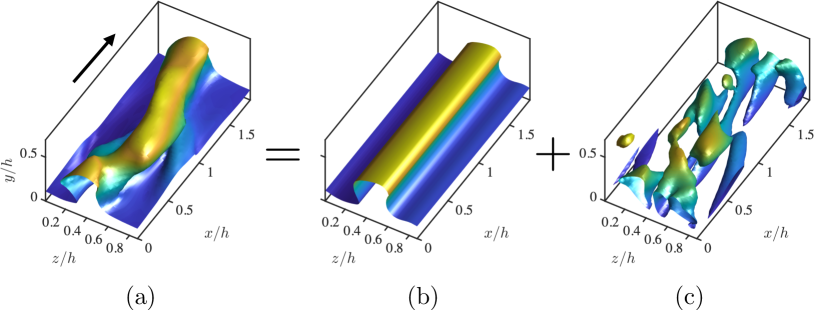
Figure 1: Decomposition of the instantaneous flow into a streamwise mean base state and fluctuations. Instantaneous isosurface of streamwise velocity for (a) the total flow $u$, (b) the streak base state $U$, and (c) the absolute value of the fluctuations $|u^{\prime}|$. The values of the isosurfaces are 0.8 (a and b) and 0.1 (c) of the maximum streamwise velocity. Colors represent the distance to the wall located at $y=0$. The arrow in panel (a) indicates the mean flow direction.

To investigate the role of modal instabilities, we examine data from spatially and temporally resolved simulations of an incompressible turbulent channel flow driven by a constant mean pressure gradient. Hereafter, the streamwise, wall-normal, and spanwise directions of the channel are denoted by $x$, $y$, and $z$, respectively, and the corresponding flow velocity components and pressure by $u$, $v$, $w$, and $p$. The density of the fluid is $\rho$ and the channel height is $h$. The wall is located at $y=0$, where no-slip boundary conditions apply, whereas free stress and no penetration conditions are imposed at $y=h$. The streamwise and spanwise directions are periodic. The grid resolution of the simulations in $x$, $y$, and $z$ is $64\times 90\times 64$, respectively, which is fine enough to resolve all the scales of the fluid motion. Additional details on the numerical setup are offered in Ref. Lozano-Durán et al. (2018).

The simulations are characterized by the non-dimensional Reynolds number, defined as the ratio between the largest and the smallest length-scales of the flow, $h$ and $\delta_{v}=\nu/u_{\tau}$, respectively, where $\nu$ is the kinematic viscosity of the fluid and $u_{\tau}$ is the characteristic velocity based on the friction at the wall (Pope, 2000). The Reynolds number selected is $\mathrm{Re}_{\tau}=\delta/\delta_{v}\approx 180$, which provides a sustained turbulent flow at an affordable computational cost (Kim et al., 1987). The flow is simulated for $100h/u_{\tau}$ units of time, which is orders of magnitude longer than the typical lifetime of individual energy-containing eddies (Lozano-Durán and Jiménez, 2014). The streamwise, wall-normal, and spanwise sizes of the computational domain are $L_{x}^{+}\approx 337$, $L_{y}^{+}\approx 184$, and $L_{z}^{+}\approx 168$, respectively, where the superscript $+$ denotes quantities normalized by $\nu$ and $u_{\tau}$. Jiménez and Moin Jiménez and Moin (1991) showed that turbulence in such domains contains an elemental flow unit comprised of a single streamwise streak and a pair of staggered quasi-streamwise vortices, that reproduce the dynamics of the flow in larger domains. Hence, the current numerical experiment provides a fundamental testbed for studying the self-sustaining cycle of wall turbulence.

We focus on the dynamics of the fluctuating velocities $\bm{u}^{\prime}\equiv(u^{\prime},v^{\prime},w^{\prime})$, defined with respect to the streak base state $U(y,z,t)\equiv L_{x}^{-1}\int_{0}^{L_{x}}u(x,y,z,t)\,\mathrm{d}x$, such that $u^{\prime}\equiv u-U$, $v^{\prime}\equiv v$, and $w^{\prime}\equiv w$. The fluctuating state vector $\bm{q}^{\prime}\equiv(u^{\prime},v^{\prime},w^{\prime},p^{\prime}/\rho u_{\tau})$ is governed by

$$\mathcal{P}\frac{\partial\bm{q}^{\prime}}{\partial t}=\mathcal{A}(U)\bm{q}^{\prime}+\bm{N}(\bm{q}^{\prime}),$$ (1)

where $\mathcal{A}$ is the linearized Navier–Stokes operator for the fluctuating state vector about the instantaneous $U(y,z,t)$ (see Fig. 1b), the operator $\mathcal{P}$ accounts for the kinematic divergence-free condition $\bm{\nabla}\cdot\bm{u}^{\prime}=0$, and $\bm{N}$ collectively denotes the nonlinear terms (which are quadratic with respect of fluctuating flow fields). The corresponding equation of motion for $U(y,z,t)$ is obtained by averaging the Navier–Stokes equations in the streamwise direction.

The modal instabilities of the streaks at a given time are obtained by eigenanalysis of the matrix representation of the operator $\mathcal{A}$ about the instantaneous $U$,

$$\mathcal{A}(U)=\mathcal{Q}\Sigma\mathcal{Q}^{-1},$$ (2)

where $\mathcal{Q}$ consists of the eigenvectors organized in columns and $\Sigma$ is the diagonal matrix of associated eigenvalues, $\sigma_{i}$. The streak is unstable when the growth rate $\lambda_{i}\equiv\mathrm{Real}(\sigma_{i})$ is positive. Figure 2 shows a representative example of the streamwise velocity of an unstable eigenmode. The predominant eigenmode has the typical sinuous structure of positive and negative patches of velocity flanking the velocity streak side by side, which may lead to its subsequent meandering and breakdown.

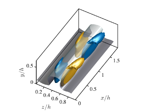
Figure 2: Isosurface of the instantaneous streamwise velocity for the eigenmode associated with the most unstable eigenvalue $\lambda_{\mathrm{max}}h/u_{\tau}\approx 3$ at $t=5.1h/u_{\tau}$. The values of the isosurface are $-0.5$ (blue) and $0.5$ (yellow) of the maximum streamwise velocity. The transparent gray isosurface shows the streak at the same instance from Fig. 1(b).

We consider two numerical experiments. First, we simulate the Navier–Stokes equations without any modification, in which the modal growth of perturbations is naturally allowed. We refer to this case as the “regular channel.” On average, the operator $\mathcal{A}$ contains 2 to 3 unstable eigenmodes at a given instant. Figure 3(a) shows the evolution of the maximum growth rate supported by $\mathcal{A}$ and denoted by $\lambda_{\mathrm{max}}$. The flow is modally unstable ($\lambda_{\mathrm{max}}>0$) 70% of the time. The corresponding kinetic energy of the perturbations averaged over the channel is shown in Fig. 3(b).

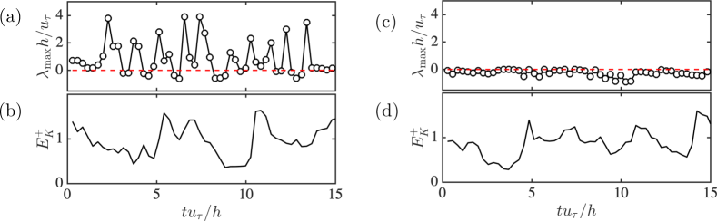
Figure 3: (a,c) The evolution of the most unstable eigenvalue $\lambda_{\rm max}$ of (a) $\mathcal{A}$ for the regular channel flow and (c) $\tilde{\mathcal{A}}$ for the channel flow with suppressed modal instabilities. (b,d) The evolution of the kinetic energy of the perturbations $E_{K}=\bm{u}^{\prime}\cdot\bm{u}^{\prime}/2$ averaged over the channel domain for (b) the regular channel flow and (d) for the channel flow with suppressed modal instabilities.

For the second numerical experiment, we modify the operator $\mathcal{A}$ so that all the unstable eigenmodes are rendered neutral for all times. We refer to this case as the “channel with suppressed modal instabilities” and we inquire whether turbulence is sustained in this case. The approach is implemented by replacing $\mathcal{A}$ at each time-instance by the modally-stable operator

$$\tilde{\mathcal{A}}=\mathcal{Q}\tilde{\Sigma}\mathcal{Q}^{-1},$$ (3)

where $\tilde{\Sigma}$ is the stabilized version of $\Sigma$ obtained by setting the real part of all unstable eigenvalues of $\Sigma$ equal to zero. We do not modify the equation of motion for $U(y,z,t)$. The stable counterpart of $\mathcal{A}$ in Eq. (3), $\tilde{\mathcal{A}}$, represents the smallest intrusion into the system to achieve modally stable wall turbulence at all times while leaving other linear mechanisms almost intact. Figure 3(c) shows the maximum modal growth rate of $\tilde{\mathcal{A}}$ at selected times with the instabilities successfully neutralized. It was verified that turbulence persists when $\mathcal{A}$ is replaced by $\tilde{\mathcal{A}}$ (Fig. 3d).

Our main result is presented in Fig. 4, which compares the mean velocity profile and turbulence intensities for both the regular channel and the channel with suppressed modal instabilities. The statistics are compiled for the statistical steady state after initial transients. Notably, the turbulent channel flow without modal instabilities is capable of sustaining turbulence. The difference of roughly 15%–25% in the turbulence intensities between cases indicates that, even if the linear instability of the streak manifests in the flow, it is not a requisite for maintaining turbulent fluctuations. The new flow equilibrates at a state with augmented streamwise fluctuations (Fig. 4b) and depleted cross flow (Fig. 4c,d). The outcome is consistent with the occasional inhibition of the streak meandering or breakdown via modal instability, which enhances the streamwise velocity fluctuations, whereas wall-normal and spanwise turbulence intensities are diminished due to a lack of vortices succeeding the collapse of the streak.

Figure 4: (a) Streamwise mean velocity profile as a function of the wall-normal distance and (b) streamwise, (c) wall-normal, and (d) spanwise root-mean-squared fluctuating velocities for the regular channel (            ) and the channel with suppressed modal instabilities (   ). The Reynolds number of both simulations is $\mathrm{Re}_{\tau}=186$. Angle brackets represent averaging in the homogeneous directions and time.

In summary, we have investigated the linear mechanism of energy injection from the streamwise-averaged mean flow to the turbulent fluctuations by modal instabilities. We have devised a numerical experiment of a turbulent channel flow in which the linear operator is altered to render any modal instabilities of the streaks stable, thus precluding the energy transfer from the mean to the fluctuations via exponential growth. Our results establish that wall turbulence with realistic mean velocity and turbulence intensities persists even when modal instabilities are suppressed. Therefore, we conclude that modal instabilities of the streaks are not required to attain a self-sustaining cycle in wall-bounded turbulence. The present outcome is consequential to comprehend, model, and control the structure of wall-bounded turbulence by linear methods (e.g., Refs. Högberg et al. (2003); Del Álamo and Jiménez (2006); Hwang and Cossu (2010); Morra et al. (2019)).

Our conclusions refer to the dynamics of wall turbulence in channels computed using minimal flow units, chosen as simplified representations of naturally occurring wall turbulence. The approach presented in this Letter paves the path for future investigations at high-Reynolds-numbers turbulence obtained for larger unconstraining domains, in addition to extensions to different flow configurations in which the role of modal instabilities remains elusive.

A.L.-D. acknowledges the support of the NASA Transformative Aeronautics Concepts Program (Grant No. NNX15AU93A) and the Office of Naval Research (Grant No. N00014-16-S-BA10). N.C.C. was supported by the Australian Research Council (Grant No. CE170100023). This work was also supported by the Coturb project of the European Research Council (ERC-2014.AdG-669505) during the 2019 Coturb Turbulence Summer Workshop at the Universidad Politécnica de Madrid. We thank Brian Farrell, Petros Ioannou, Jane Bae, and Javier Jiménez for insightful discussions.

References

- Jiménez (2013) J. Jiménez, Phys. Fluids 25, 110814 (2013).
- Kim and R. Bewley (2006) J. Kim and T. R. Bewley, Annu. Rev. Fluid Mech. 39, 383 (2006).
- Schmid and Henningson (2012) P. Schmid and D. Henningson, Stability and Transition in Shear Flows, Applied Mathematical Sciences (Springer New York, 2012).
- Hamilton et al. (1995) J. M. Hamilton, J. Kim, and F. Waleffe, J. Fluid Mech. 287, 317 (1995).
- Waleffe (1997) F. Waleffe, Phys. Fluids 9, 883 (1997).
- Hwang and Cossu (2011) Y. Hwang and C. Cossu, Phys. Fluids 23, 061702 (2011).
- Schoppa and Hussain (2002) W. Schoppa and F. Hussain, J. Fluid Mech. 453, 57 (2002).
- Del Álamo and Jiménez (2006) J. C. Del Álamo and J. Jiménez, J. Fluid Mech. 559, 205 (2006).
- Hwang and Cossu (2010) Y. Hwang and C. Cossu, J. Fluid Mech. 664, 51 (2010).
- Klebanoff et al. (1962) P. S. Klebanoff, K. D. Tidstrom, and L. M. Sargent, J. Fluid Mech. 12, 1 (1962).
- Kline et al. (1967) S. J. Kline, W. C. Reynolds, F. A. Schraub, and P. W. Runstadler, J. Fluid Mech. 30, 741 (1967).
- Panton (2001) R. L. Panton, Prog. Aerosp. Sci. 37, 341 (2001).
- Adrian (2007) R. J. Adrian, Phys. Fluids 19, 041301 (2007).
- Smits et al. (2011) A. J. Smits, B. J. McKeon, and I. Marusic, Annu. Rev. Fluid Mech. 43, 353 (2011).
- Jiménez (2012) J. Jiménez, Annu. Rev. Fluid Mech. 44, 27 (2012).
- Jiménez (2018) J. Jiménez, J. Fluid Mech. 842, P1 (2018).
- Kim et al. (1971) J. Kim, S. J. Kline, and W. C. Reynolds, J. Fluid Mech. 50, 133 (1971).
- Jiménez and Moin (1991) J. Jiménez and P. Moin, J. Fluid Mech. 225, 213 (1991).
- Butler and Farrell (1993) K. M. Butler and B. F. Farrell, Phys. Fluids A 5, 774 (1993).
- Farrell and Ioannou (2012) B. F. Farrell and P. J. Ioannou, J. Fluid Mech. 708, 149 (2012).
- Farrell et al. (2016) B. F. Farrell, P. J. Ioannou, J. Jiménez, N. C. Constantinou, A. Lozano-Durán, and M.-A. Nikolaidis, J. Fluid Mech. 809, 290 (2016).
- Lozano-Durán et al. (2018) A. Lozano-Durán, M. Karp, and N. C. Constantinou, in Center for Turbulence Research – Annual Research Briefs (2018) pp. 209–220.
- Andersson et al. (2001) P. Andersson, L. Brandt, A. Bottara, and D. S. Henningson, J. Fluid Mech. 428, 29 (2001).
- Kawahara et al. (2003) G. Kawahara, J. Jiménez, M. Uhlmann, and A. Pinelli, J. Fluid Mech. 483, 315 (2003).
- Hack and Zaki (2014) M. J. P. Hack and T. A. Zaki, J. Fluid Mech. 741, 280 (2014).
- Hack and Moin (2018) M. J. P. Hack and P. Moin, J. Fluid Mech. 844, 917 (2018).
- Pope (2000) S. B. Pope, Turbulent Flows (Cambridge University Press, 2000).
- Kim et al. (1987) J. Kim, P. Moin, and R. Moser, J. Fluid Mech. 177, 133 (1987).
- Lozano-Durán and Jiménez (2014) A. Lozano-Durán and J. Jiménez, J. Fluid. Mech. 759, 432 (2014).
- Högberg et al. (2003) M. Högberg, T. R. Bewley, and D. S. Henningson, J. Fluid Mech. 481, 149 (2003).
- Morra et al. (2019) P. Morra, O. Semeraro, D. S. Henningson, and C. Cossu, J. Fluid Mech. 867, 969 (2019).