An Extension of Fast Iterative Shrinkage-thresholding to Riemannian Optimization for Sparse Principal Component Analysis

Abstract

Sparse principal component analysis (PCA), an important variant of PCA, attempts to find sparse loading vectors when conducting dimension reduction. This paper considers the nonsmooth Riemannian optimization problem associated with the ScoTLASS model [JTU03] for sparse PCA which can impose orthogonality and sparsity simultaneously. A Riemannian proximal method is proposed in the work of Chen et al. [CMSZ20] for the efficient solution of this optimization problem. In this paper, two acceleration schemes are introduced. First and foremost, we extend the FISTA method from the Euclidean space to the Riemannian manifold to solve sparse PCA, leading to the accelerated Riemannian proximal gradient method. Since the Riemannian optimization problem for sparse PCA is essentially non-convex, a restarting technique is adopted to stabilize the accelerated method without sacrificing the fast convergence. Second, a diagonal preconditioner is proposed for the Riemannian proximal subproblem which can further accelerate the convergence of the Riemannian proximal methods. Numerical evaluations establish the computational advantages of the proposed methods over the existing proximal gradient methods on a manifold. Additionally, a short result concerning the convergence of the Riemannian subgradients of a sequence is established, which, together with the result in the work of Chen et al. [CMSZ20], can show the stationary point convergence of the Riemannian proximal methods.

1 Introduction

Principal component analysis (PCA) is an important data processing technique. In essence, PCA attempts to find a low dimensional representation of a data set. The low dimensional representation can be subsequently used for data denoising, vision and recognition, just to name a few. However, due to the complexity of data as well as the interpretability issues, vanilla PCA may not be able to meet the requirements of real applications. Therefore, several variants of PCA have been proposed and studied, one of which is sparse PCA.

Given a dataset, PCA aims to find linear combinations of the original variables such that the new variables can capture the maximal variance in the data. In order to achieve the maximal variance, PCA tends to use a linear combination of all the variables. Thus, all coefficients (loadings) in the linear combination are typically non-zero, which will cause interpretability issues in many applications. For example, in genome data analysis, each coefficient may correspond to a specific gene, and it is more desirable to have the new variable being composed of only a few genes. This means that the loading vector should have very few non-zero entries.

Let $A$ be an $m\times n$ data matrix, where $m$ denotes the number of samples and $n$ denotes the number of variables. Without loss of generality, assume each column of $A$ has zero mean. Then PCA can be formally expressed as the following maximization problem:

$$\max_{X\in\mathbb{R}^{n\times p}}\|AX\|_{\mathrm{F}}^{2}\quad\mbox{subject to}\quad X^{T}X=I_{p},$$ (1.1)

where each column $X$ denotes a loading vector. The PCA problem admits a closed form solution which can be computed via the singular value decomposition (SVD) of the data matrix. However, it seldom yields a sparse solution; that is, each column of $X$ is very likely to be a dense vector. Alternatively, sparse PCA attempts to achieve a better trade-off between the variance of $AX$ and the sparsity of $X$. In this paper we consider the following model for sparse PCA:

$$\min_{X\in\mathbb{R}^{n\times p}}-\|AX\|_{\mathrm{F}}^{2}+\lambda\|X\|_{1}\quad\mbox{subject to}\quad X^{T}X=I_{p},$$ (1.2)

where $\|X\|_{1}=\sum_{i,j}|X_{ij}|$ imposes the sparsity of $X$ and $\lambda>0$ is a tuning parameter controlling the balance between variance and sparsity.

In fact, (1.2) is a penalized version of the ScoTLASS model proposed by Jolliffe et al. [JTU03], which is inspired by the Lasso regression. In addition to the ScoTLASS model, there are many other formulations for sparse PCA. By rewriting PCA as a regression optimization problem, Zou et al. [ZHT06] propose a model which mixes the ridge regression and the Lasso regression. A semidefinite programming is proposed in the work of d’Aspremont et al. [dBG08, dGJL07] to compute the dominant sparse loading vector. In the work of Shen and Huang[SH08] and Witten et al. [WTH09], sparse PCA is studied based on matrix decompositions. A formulation similar to (1.2) but with decoupled variables is investigated in [JNRS10]. Moreover, different algorithms have been developed for different formulations. We refer interested readers to [ZX18] for a nice overview of sparse PCA on both computational and theoretical results.

Due to the simultaneous existence of the orthogonal constraint and the non-smooth term in (1.2), it is quite challenging to develop fast algorithms to compute its solution. In the work of Chen et al. [CMSZ20], a Riemannian proximal gradient method called ManPG is proposed for this problem. In this paper we extend the fast iterative shrinkage-thresholding algorithm (FISTA[BT09]) to solve (1.2). For ease of exposition, we consider the following more general nonconvex optimization problem:

$$\min F(x)=f(x)+g(x)\quad\mbox{subject to}\quad x\in\mathcal{M},$$ (1.3)

where $\mathcal{M}\subset\mathbb{R}^{n\times m}$ is a compact Riemannian submanifold, $f:\mathbb{R}^{n\times m}\rightarrow\mathbb{R}$ is $L$-continuously differentiable (may be nonconvex) and $g$ is continuous, convex, but may be nondifferentiable. Clearly, (1.2) is a special case of (1.3) with $\mathcal{M}$ being the Stiefel manifold, defined by

$$\operatorname{\mathrm{St}}(p,n)=\{X\in\mathbb{R}^{n\times p}~{}|~{}X^{T}X=I_{p}\}.$$ (1.4)

When $F$ is a smooth function (i.e., $g=0$), most of the standard optimization algorithms for the Euclidean setting, for example the (accelerated) gradient method, the Newton method and the BFGS method, and the trust region method, are readily extended to the Riemannian setting; see the work[AMS08, Hua13, Van10, Bou14, Mis14] and references therein.

There have also been many algorithms that are designed for the nonsmooth optimization problems on manifold. In the work of Ferreira and Oliveira[FO98], a subgradient method is studied for minimizing a convex function on a Riemannian manifold and convergence guarantee is established for the diminishing stepsizes. In the paper [ZS16], Zhang and Sra analyze a Riemannian subgradient-based method and show that the cost function decreases to the optimal value at the rate of $O(1/\sqrt{k})$. When the cost function is Lipschitz continuous, the $\epsilon$-subgradient method is a variant of the subgradient method which utilizes the gradient at nearby points as an approximation of the subgradient at a given point. In the papers [GH15a, GH15b], Grohs and Hosseini develop two $\epsilon$-subgradient-based optimization methods using line search strategy and trust region strategy, respectively. The convergence of the algorithms to critical points is established in their work. Huang [Hua13] generalizes a gradient sampling method to the Riemannian setting, which is very efficient for small-scale problems but lacks convergence analysis. In the paper [HU17], Hosseini and Uschmajew present a Riemannian gradient sampling method with convergence analysis. Recently, Hosseini et al. [HHY18] propose a new Riemannian line search method by combining the $\epsilon$-subgradient method and the quasi-Newton ideas. The proximal point method has also been extended to the Riemannian setting. For instance, Ferreira and Oliveira propose a Riemannian proximal point method [FO02]. The $O(1/k)$ convergence rate of the method for the Hadamard manifold is established by Bento et al.  [BFM17]. The shortcoming of the Riemannian proximal point method is that there do not exist efficient algorithms for the subproblems.

While some of the aforementioned algorithms are also applicable for the nonsmooth optimization problem (1.3), they lack the ability of exploiting the decomposable structure of the cost function. In contrast, a proximal gradient method (ManPG) is proposed in the work of Chen et al. [CMSZ20] when $\mathcal{M}$ is the Stiefel manifold in (1.3), which is an analogue of the proximal gradient method in the Euclidean setting and hence is able to take advantage of the problem structure. Moreover, Riemannian proximal methods for composite problems on general manifolds are developed in the work of the same authors [HW21] based on a different Riemannian proximal mapping. As suggested in that work, for optimization problems on Stiefel manifold (the focus of this paper), the solution to the Riemannian proximal mapping used in the work of Chen et al.  [CMSZ20] and this paper can be solved more efficiently.

The main contributions of this paper are summarized as follows. We first extend the accelerated proximal gradient method (specifically FISTA [BT09]) to the Riemannian setting to solve (1.3). The algorithm is coined as AManPG (accelerated ManPG ). A simple safeguard is introduced in AManPG so that its convergence to stationary points can be guaranteed. Empirical comparisons clearly show that as in the Euclidean case AManPG exhibits a faster convergence rate than ManPG. Moreover, a weighted proximal subproblem is considered in this paper and we observe that a computationally efficient weight in the diagonal form can further speed up the Riemannian proximal gradient methods. It has been shown in the work [CMSZ20] that the search direction computed in ManPG converges to zero. In this paper a complementary result about the convergence of the Riemannian subgradients of a sequence is provided, which can be used to complete the stationary point analysis of the Riemannian proximal methods together with the result in the work [CMSZ20].

The remainder of this paper is organized as follows. In Section 2, we give some basic facts about Riemannian manifolds and Riemannian optimization. The accelerated Riemannian proximal gradient method (i.e., AManPG) is presented in Section 3 together with the preliminary convergence analysis. Empirical performance evaluations are presented in 4, while Section 5 concludes this paper with a few future directions.

2 Preliminaries on Manifold

This section reviews some basic notation on Riemannian manifold that is closely related to the work in this paper. We focus on submanifolds of Euclidean spaces with $\operatorname{\mathrm{St}}(p,n)$ as an example since in this case the manifold is geometrically more intuitive and can be imagined as a smooth surface in a 3D space. Interested readers are referred to the book[AMS08] for more details about Riemannian manifolds and Riemannian optimization.

Assume $\mathcal{M}$ is a smooth submanifold of a Euclidean space and let $x\in\mathcal{M}$. The tangent space of $\mathcal{M}$ at $x$, denoted $\operatorname{\mathrm{T}}_{x}\mathcal{M}$, is a collection of derivatives of all the smooth curves passing through $x$,

$$\operatorname{\mathrm{T}}_{x}\mathcal{M}=\{\gamma^{\prime}(0)~{}|~{}\gamma(t)\mbox{ is a curve in }\mathcal{M}\mbox{ with }\gamma(0)=x\}.$$

The tangent space is a vector space and each tangent vector in $\operatorname{\mathrm{T}}_{x}\mathcal{M}$ corresponds to a linear mapping from the set of smooth real-valued functions in a neibourghood of $x$ to $\mathbb{R}$. Indeed, it is the latter property that is adopted to define tangent spaces for abstract manifolds. Since $\operatorname{\mathrm{T}}_{x}\mathcal{M}$ is a vector space, we can equip it with an inner product (or metric) $g_{x}(\cdot,\cdot):\operatorname{\mathrm{T}}_{x}\mathcal{M}\times\operatorname{\mathrm{T}}_{x}\mathcal{M}\rightarrow\mathbb{R}$; see Figure 1 (left) for an illustration. A manifold whose tangent spaces are endowed with a smoothly varying metric is referred to as a Riemannian manifold. For a smooth function $f$ defined a Riemannian manifold, the Riemannian gradient of $f$ at $x$, denoted $\operatorname{\mathrm{grad}}f(x)$, is the unique tangent vector such that $g_{x}(\operatorname{\mathrm{grad}}f(x),\eta_{x})=\operatorname{\mathrm{D}}f(x)[\eta_{x}],~{}\forall\eta_{x}\in\operatorname{\mathrm{T}}_{x}\mathcal{M}$, where $\operatorname{\mathrm{D}}f(x)[\eta_{x}]$ is the directional derivative of $f$ along the direction $\eta_{x}$. Moreover, the Riemannian gradient of $f$ at $x$ is simply the orthogonal projection of $\nabla f(x)$ onto $\operatorname{\mathrm{T}}_{x}\mathcal{M}$; that is,

$$\operatorname{\mathrm{grad}}f(x)=\mathrm{P}_{\operatorname{\mathrm{T}}_{x}\mathcal{M}}\nabla f(x),$$ (2.1)

where $\nabla f(x)$ is the Euclidean gradient of $f$ at $x$.

When we construct the diagonal weight for the proximal subproblem in the algorithm, the second order information of a function on the Riemannian manifold will also be needed. The Riemannian Hessian of $f$ at $x$, denoted $\operatorname{\mathrm{Hess}}f(x)$, is a mapping from $\operatorname{\mathrm{T}}_{x}\mathcal{M}$ to $\operatorname{\mathrm{T}}_{x}\mathcal{M}$. Moreover, when $\mathcal{M}$ is a Riemannian submanifold of a Euclidean space $\operatorname{\mathrm{Hess}}f(x)$ satisfies

$$\operatorname{\mathrm{Hess}}f(x)[\eta_{x}]=\mathrm{P}_{\operatorname{\mathrm{T}}_{x}\mathcal{M}}\operatorname{\mathrm{D}}\operatorname{\mathrm{grad}}f(x)[\eta_{x}],\quad\eta_{x}\in\operatorname{\mathrm{T}}_{x}\mathcal{M},$$ (2.2)

where $\operatorname{\mathrm{D}}\operatorname{\mathrm{grad}}f(x)[\eta_{x}]$ denotes the directional derivative of $\operatorname{\mathrm{grad}}f(x)$ along the direction $\eta_{x}$.

Figure 1: (Left) Riemannian metric; (Right) Retraction.

Regarding the Stiefel manifold, the tangent space of $\operatorname{\mathrm{St}}(p,n)$ at a matrix $X$ is given by

$$\operatorname{\mathrm{T}}_{X}\operatorname{\mathrm{St}}(p,n)=\{\eta_{X}\in\mathbb{R}^{n\times p}~{}|~{}X^{T}\eta_{X}+\eta_{X}^{T}X=0\}.$$ (2.3)

In particular, when $p=1$, $\operatorname{\mathrm{St}}(p,n)$ is the unit sphere $\mathbb{S}^{n-1}$ in $\mathbb{R}^{n}$ and $\operatorname{\mathrm{T}}_{x}\mathbb{S}^{n-1}$ consists of those vectors that are perpendicular to $x$. We can use the inner product inherited from $\mathbb{R}^{n\times p}$ as the Riemannian metric on $\operatorname{\mathrm{T}}_{X}\operatorname{\mathrm{St}}(p,n)$; that is,

$$g_{X}(\xi_{X},\eta_{X})=\operatorname{\mathrm{trace}}(\xi_{X}^{T}\eta_{X}),\quad\forall~{}\xi_{X},\eta_{X}\in\operatorname{\mathrm{T}}_{X}\operatorname{\mathrm{St}}(p,n).$$

Under this metric, the projection of any $n\times p$ matrix $\xi$ onto $\operatorname{\mathrm{T}}_{X}\operatorname{\mathrm{St}}(p,n)$ is given by

$$\mathrm{P}_{\operatorname{\mathrm{T}}_{X}\operatorname{\mathrm{St}}(p,n)}=\xi-X\mbox{sym}(X^{T}\xi),\quad\mbox{where }\mbox{sym}(X^{T}\xi)=\frac{X^{T}\xi+\xi^{T}X}{2}.$$ (2.4)

A Riemannian optimization algorithm typically conducts a line search or solves a linear system or a model problem on a tangent space, and then moves the solution back to the manifold. The notion of retraction plays a key role in mapping vectors in a tangent space to points on a manifold.

Definition 2.1 (Retraction).

At $x\in\mathcal{M}$, a retraction $R_{x}(\cdot)$ is a smooth mapping from $\operatorname{\mathrm{T}}_{x}\mathcal{M}$ to $\mathcal{M}$ which satisfies the following two properties: 1) $R_{x}(0_{x})=x$, where $0_{x}$ is the zero element in $\operatorname{\mathrm{T}}_{x}\mathcal{M}$; 2) $\left.\frac{d}{dt}R_{x}(t\eta_{x})\right|_{t=0}=\xi_{x}$ for any $\xi_{x}\in\operatorname{\mathrm{T}}_{x}\mathcal{M}$.

The second property means the velocity of the curve defined by $R_{x}(t\eta_{x})$ is equal to $\eta_{x}$ at $t=0$; see Figure 1 (right). Roughly speaking, retraction plays the role of line search when designing a Riemannian optimization algorithm; namely,

$$\mbox{(Euclidean) }x_{k+1}=x_{k}+\eta_{x_{k}}\quad\Rightarrow\quad\mbox{(Riemannian) }x_{k+1}=R_{x_{k}}(\eta_{x_{k}}).$$ (2.5)

Note that the two properties in Definition 2.1 cannot uniquely determine a retraction. For the Stiefel manifold, several retractions can be constructed, for example those based on the exponential map, the QR factorization, the singular value decomposition (SVD) or the polar decomposition [AMS08]. In this paper we use the one based on the SVD:

$$R_{X}(\eta_{X})=UV^{T},\quad\mbox{where }X+\eta_{X}=U\Sigma V^{T}\mbox{ is the SVD of }X+\eta_{X}.$$

Noticing that $X\in\operatorname{\mathrm{St}}(p,n)$ and $\eta_{X}\in\operatorname{\mathrm{T}}_{X}\operatorname{\mathrm{St}}(p,n)$, thus $X+\eta_{X}$ is a matrix of full column rank. Then it is not hard to verify that the retraction based on the SVD is equivalent to the retraction based on the polar decomposition given by

$$R_{X}(\eta_{X})=(X+\eta_{X})(I_{p}+\eta_{X}^{T}\eta_{X})^{-1/2}.$$ (2.6)

Since $X+\eta_{X}$ is a tall matrix, an alternative way to compute $R_{X}(\eta_{X})$ is as follows:

$$[Q,R]=\mbox{qr}(X+\eta_{X}),~{}[\tilde{U},\tilde{S},\tilde{V}]=\mbox{svd}(R),~{}R_{X}(\eta_{X})=Q(\tilde{U}\tilde{V}^{T}),$$ (2.7)

where qr and svd means computing the compact QR decomposition and SVD of a matrix, respectively.

When the cost function $F$ of the Riemannian optimization problem is smooth, the first order optimality condition is

$$\operatorname{\mathrm{grad}}F(x)=0.$$

If $F$ is not differentiable but Lipschitz continuous, then the Riemannian version of generalized Clarke subdifferential introduced in Hosseini et al. [HP11, HHY18] is used. Specifically, since $\hat{F}_{x}=F\circ R_{x}$ is a Lipschitz continuous function defined on a Hilbert space $\operatorname{\mathrm{T}}_{x}\mathcal{M}$, the generalized Clarke directional derivative at $\eta_{x}\in\operatorname{\mathrm{T}}_{x}\mathcal{M}$, denoted by $\hat{F}_{x}^{\circ}(\eta_{x};v)$, is defined by

$$\hat{F}_{x}^{\circ}(\eta_{x};v)=\lim_{\xi_{x}\rightarrow\eta_{x}}\sup_{t\downarrow 0}\frac{\hat{F}_{x}(\xi_{x}+tv)-\hat{F}_{x}(\xi_{x})}{t},$$

where $v\in\operatorname{\mathrm{T}}_{x}\mathcal{M}$. The generalized Clarke subdifferential of $\hat{F}_{x}$ at $\eta_{x}$, denoted by $\partial\hat{F}_{x}(\eta_{x})$, is defined by

$$\partial\hat{F}_{x}(\eta_{x})=\{\eta_{x}\in\operatorname{\mathrm{T}}_{x}\mathcal{M}\mid{\langle\eta_{x},v\rangle_{x}}\leq\hat{F}_{x}^{\circ}(\eta_{x};v)\hbox{ for all }v\in\operatorname{\mathrm{T}}_{x}\mathcal{M}\}.$$

The Riemannian version of generalized Clarke subdifferential of $F$ at $x$, denoted $\hat{\partial}F(x)$, is defined as $\hat{\partial}F(x)=\partial\hat{F}_{x}(0_{x})$. Any tangent vector $\xi_{x}\in\hat{\partial}F(x)$ is called a subgradient of $F$ at $x$. For the cost function in (1.3) (or a class of regular functions in general), the generalized Clarke subdifferential is given by [YZR14]

$$\hat{\partial}F(x)=\mathrm{P}_{\operatorname{\mathrm{T}}_{X}\mathcal{M}}\partial F(x),$$

where $\partial F(x)$ denotes the subdifferential in the Euclidean space. Moreover, the first order optimality of the problem (1.3) is given by

$$0\in\hat{\partial}F(x)=\operatorname{\mathrm{grad}}f(x)+\mathrm{P}_{\operatorname{\mathrm{T}}_{X}\mathcal{M}}\partial g(x).$$

We refer the reader to the work of Yang et al. [YZR14] for more details.

3 Extending FISTA to Riemannian Optimization

Before presenting the algorithm for (1.3), let us first briefly review the proximal gradient method and accelerated proximal gradient method for the optimization problem similar to (1.3) but with the manifold constraint $x\in\mathcal{M}$ being dropped. In each iteration, the proximal gradient method updates the estimate of the minimizer via

$$\begin{cases}\eta_{x_{k}}=\operatorname*{arg\,min}_{\eta\in\mathbb{R}^{n\times p}}\langle\nabla f(x_{k}),\eta\rangle+\frac{1}{2\mu}\|\eta\|_{\mathrm{F}}^{2}+g(x_{k}+\eta)\\ x_{k+1}=x_{k}+\eta_{x_{k}},\end{cases}$$ (3.1)

where $\|\eta\|_{\mathrm{F}}$ denotes the Frobenius norm of $\eta$. In many practical settings, the proximal mapping either has a closed-form solution or can be solved efficiently. Thus, the algorithm has low per iteration cost and is applicable for large-scale problems. Furthermore, under the assumptions that $f$ is convex, Lipschitz-continuously differentiable with Lipschitz constant $L$, $g$ is convex, and $F$ is coercive, the proximal gradient method converges on the order of $O(1/k)$ [BT09, Bec17]. Note that the convergence rate of the proximal gradient method is not optimal and algorithms achieving the optimal $O(1/k^{2})$ [Dar83, Nes83] convergence rate can be developed based on certain acceleration schemes. In the paper[BT09], Beck and Teboulle present an accelerated proximal gradient method (known as FISTA) based on the Nesterov momentum technique. The algorithm consists of the following steps

$$\begin{cases}\eta_{y_{k}}=\operatorname*{arg\,min}_{\eta\in\mathbb{R}^{n\times p}}\langle\nabla f(y_{k}),\eta\rangle+\frac{1}{2\mu}\|\eta\|_{\mathrm{F}}^{2}+g(y_{k}+\eta)\\ x_{k+1}=y_{k}+\eta_{y_{k}}\\ t_{k+1}=\frac{\sqrt{4t_{k}^{2}+1}+1}{2}\\ y_{k+1}=x_{k+1}+\frac{t_{k}-1}{t_{k+1}}(x_{k+1}-x_{k}).\end{cases}$$ (3.2)

Under the same conditions as in the convergence analysis of the proximal gradient method, FISTA been proven to converge on the order of $O(1/k^{2})$ [BT09].

In the work of Chen et al. [CMSZ20], the Manifold Proximal Gradient method (ManPG) is proposed to solve (1.3). The structure of the algorithm is overall is similar to (3.1), except that a subproblem constrained to the tangent space is solved. More precisely, the following constrained optimization problem is first solved to compute the search direction,

$$\eta_{x_{k}}=\operatorname*{arg\,min}_{\eta\in\operatorname{\mathrm{T}}_{x_{k}}\mathcal{M}}\langle\operatorname{\mathrm{grad}}f(x_{k}),\eta\rangle+\frac{1}{2\mu}\|\eta\|_{{}{W_{x_{k}}}}^{2}+g(x_{k}+\eta),$$ (3.3)

where $\|\eta\|_{{}{W_{x}}}^{2}=\langle\eta,{}{W_{x}}\eta\rangle$ with ${}{W_{x}}:\operatorname{\mathrm{T}}_{x}\mathcal{M}\rightarrow\operatorname{\mathrm{T}}_{x}\mathcal{M}$ being a symmetric, positive definite linear operator. Here we describe the proximal subproblem in a more general form by introducing a weight operator. As will be seen in the simulations, a simple diagonal weight that is computed adaptively can help improve the convergence of the algorithms. It is trivial that when ${}{W_{x}}$ is an identity operator, (3.3) reduces to the standard proximal subproblem considered in the work of Chen et al. [CMSZ20]. After the search direction is found, a new estimate is then computed via backtracking and retraction. Since $g(x)$ is a convex function and $\operatorname{\mathrm{T}}_{x}\mathcal{M}$ is a linear subspace, (3.3) is indeed a convex programming. Thus there are computationally efficient algorithms for this problem. We will return to this issue later in Section 3.2.

The global convergence of the algorithm has been established in the work of Chen et al. [CMSZ20]. More precisely, the authors show that the norm of the search direction computed from the Riemannian proximal mapping goes to zero. In addition, if there exists a point such that the search direction from this point vanishes, then this point must be a critical point.

Algorithm 1 Accelerated Manifold Proximal Gradient Method (AManPG)

1:Lipschitz constant $L$ on $\nabla f$, parameter $\mu\in(0,1/L]$ in the proximal mapping, line search parameter $\sigma\in(0,1)$, shrinking parameter in line search $\nu\in(0,1)$, positive integer $N$ for safeguard;

2:$t_{0}=1$, $y_{0}=x_{0}$, $z_{0}=x_{0}$;

3:for $k=0,\ldots$ do

4:     if $\mod(k,N)=0$ then $\triangleright$ Invoke safeguard every $N$ iterations

5:         Invoke Algorithm 2: $[z_{k+N},x_{k},y_{k},t_{k}]=Alg\ref{alg:Safeguard}(z_{k},x_{k},y_{k},t_{k},F(x_{k}))$;

6:     end if

7:     Compute

$$\eta_{y_{k}}=\operatorname*{arg\,min}_{\eta\in\operatorname{\mathrm{T}}_{y_{k}}\mathcal{M}}{\langle\operatorname{\mathrm{grad}}f(y_{k}),\eta\rangle}+\frac{1}{2\mu}\|\eta\|_{{}{W_{y_{k}}}}^{2}+g(y_{k}+\eta);$$

8:     $x_{k+1}=R_{y_{k}}(\eta_{y_{k}})$;

9:     $t_{k+1}=\frac{\sqrt{4t_{k}^{2}+1}+1}{2}$;

10:     Compute

$$y_{k+1}=R_{x_{k+1}}\left(\frac{1-t_{k}}{t_{k+1}}R_{x_{k+1}}^{-1}(x_{k})\right);$$

11:end for

Algorithm 2 Safeguard for Algorithm 1

1:$(z_{k},x_{k},y_{k},t_{k},F(x_{k}))$;

2:$[z_{k+N},x_{k},y_{k},t_{k}]$;

3: Compute

$$\eta_{z_{k}}=\operatorname*{arg\,min}_{\eta\in\operatorname{\mathrm{T}}_{z_{k}}\mathcal{M}}{\langle\operatorname{\mathrm{grad}}f(z_{k}),\eta\rangle}+\frac{1}{2\mu}\|\eta\|_{{}{W_{z_{k}}}}^{2}+g(z_{k}+\eta);$$

4:Set $\alpha=1$;

5:while $F(R_{z_{k}}(\alpha\eta_{z_{k}}))>F(z_{k})-\sigma\alpha{\|\eta_{z_{k}}\|_{\mathrm{F}}^{2}}$  do

6:     $\alpha=\nu\alpha$;

7:end while

8:if $F(R_{z_{k}}(\alpha\eta_{z_{k}}))<F(x_{k})$ then $\triangleright$ Safeguard takes effect

9:     $x_{k}=R_{z_{k}}(\alpha\eta_{z_{k}})$, $y_{k}=R_{z_{k}}(\alpha\eta_{z_{k}})$, and $t_{k}=1$;

10:else

11:     $x_{k}$, $y_{k}$ and $t_{k}$ keep unchanged;

12:end if

13:$z_{k+N}=x_{k}$; $\triangleright$ Update the compared iterate;

Inspired by the works [CMSZ20, BT09], the goal of this paper is to extend FISTA to the Riemannian setting for the optimization problem (1.3). The algorithm, dubbed Accelerated Manifold Proximal Gradient method (AManPG), is presented in Algorithm 1. According to the substitution rule provided in (2.5), the second line of (3.2) can be replaced by $R_{y_{k}}(\eta_{y_{k}})$, giving the 7th step of Algorithm 1. Moreover, the 9th step in Algorithm 1 is obtained through the following replacement:

$$y_{k+1}=\underbrace{x_{k+1}+\frac{1-t_{k}}{t_{k+1}}\underbrace{(x_{k}-x_{k+1})}_{\mbox{replaced by }R_{x_{k+1}}^{-1}(x_{k})}}_{\mbox{replaced by }R_{x_{k+1}}\left(\frac{1-t_{k}}{t_{k+1}}R_{x_{k+1}}^{-1}(x_{k})\right)},$$

where the first replacement guarantees that $R_{x_{k+1}}^{-1}(x_{k})$ is a tangent vector in $\operatorname{\mathrm{T}}_{x_{k+1}}\mathcal{M}$.

Furthermore, since we are dealing with a non-convex optimization problem, the convergence of the Riemannian version of (3.2) is not guaranteed, even for the convergence to a stationary point as the function value of the iterate does not monotonically decrease. Therefore, a safeguard strategy via restarting is introduced in Algorithm 1 to monitor the progress of the algorithm in every $N$ iterations. Whenever the safeguard rule is violated, the algorithm will be restarted. It is worth noting that the idea of restarting has also been used in the Euclidean setting to suppresses the oscillatory behaviour of the accelerated proximal gradient methods, see for example the work of O’Donoghue[OC15].

When we apply Algorithm 1 to the sparse PCA problem (1.2), the computation of the retraction is already given in (2.7). To compute the inverse of the retraction we first note that $R_{X}^{-1}(Y)$ exists when $Y$ is not far from $X$ owing to the local diffeomorphism property of retraction. Letting $\eta_{X}=R_{X}^{-1}(Y)$, by (2.6), we have $\eta_{X}=YS-X$ for $S=(I_{p}+\eta_{X}^{T}\eta_{X})^{1/2}$. Combining the fact $\eta_{X}\in\operatorname{\mathrm{T}}_{X}\operatorname{\mathrm{St}}(p,n)$ and (2.3) yields

$$(X^{T}Y)S+S(Y^{T}X)=2I_{p}.$$ (3.4)

This is a Lyapunov equation which can be computed by the Bartels-Stewart algorithm using $O(p^{3})$ flops [BS72]. Once $S$ is computed from (3.4), inserting it back into $\eta_{X}=YS-X$ gives $R_{X}^{-1}(Y)$. It is worth noting that the additional computational cost incurred by the Lyapunov equation is marginal since it is very typical that $p\ll n$ in the sparse PCA problem.

3.1 Computing the diagonal weight

In this paper we will restrict our attention to the diagonal weight for two reasons. Firstly, it is easy to compute for the sparse PCA problem. Secondly, the proximal subproblem (3.3) with a diagonal weight can be solved as efficiently as that without a weight.

Roughly speaking, we will extract a diagonal weight from the expression of the Riemannian Hessian of $f$ in each iteration. In particular, when applying the Riemannian proximal gradient methods (including ManPG and AManPG) to the sparse PCA problem (1.2), a diagonal weight can be computed in the following way. Noting $f(X)=-\|AX\|_{F}^{2}$ in (1.2), by (2.1) and (2.4), we have

$$\operatorname{\mathrm{grad}}f(X) =\mathrm{P}_{\operatorname{\mathrm{T}}_{X}\mathcal{M}}(-2A^{T}AX)$$

$$=-2A^{T}AX+2X(X^{T}A^{T}AX).$$

It follows that

$$\operatorname{\mathrm{D}}\operatorname{\mathrm{grad}}f(X)[\eta_{X}] =-2A^{T}A\eta_{X}+2\eta_{X}(X^{T}A^{T}AX)$$

$$+2X(\eta_{X}^{T}A^{T}AX+X^{T}A^{T}A\eta_{X}),\quad\forall\eta_{X}\in\operatorname{\mathrm{T}}_{X}\operatorname{\mathrm{St}}(p,n).$$

Noting that $\mathrm{P}_{\operatorname{\mathrm{T}}_{X}\operatorname{\mathrm{St}}(p,n)}(X(\eta^{T}A^{T}AX+X^{T}A^{T}A\eta))=0,$ it follows from (2.2) that

$$\operatorname{\mathrm{Hess}}f(X)[\eta_{X}]=\mathrm{P}_{\operatorname{\mathrm{T}}_{X}\operatorname{\mathrm{St}}(p,n)}(-2A^{T}A\eta_{X}+2\eta_{X}(X^{T}A^{T}AX)).$$

In the Riemannian Newton’s method, the weight operator should be chosen in a way such that

$$\langle\eta_{X},W\eta_{X}\rangle=\langle\eta_{X},\operatorname{\mathrm{Hess}}f(X)[\eta_{X}]\rangle=\langle\eta_{X},-2A^{T}A\eta_{X}+2\eta_{X}(X^{T}A^{T}AX)\rangle,$$

where the second equality follows from the fact $\eta_{X}\in\operatorname{\mathrm{T}}_{X}\operatorname{\mathrm{St}}(p,n)$. After vectorization we can rewrite the third inner product as

$$\langle\eta_{X},-2A^{T}A\eta_{X}+2\eta_{X}(X^{T}A^{T}AX)\rangle=\langle\mathrm{vec}(\eta_{X}),J\mathrm{vec}(\eta_{X})\rangle,$$

where $J$ is an $np\times np$ matrix given by

$$J=-2I_{p}\otimes(A^{T}A)+2(X^{T}A^{T}AX)\otimes I_{n}.$$

Since a diagonal weight is sought here, a natural choice is to set $W$ to be the diagonal part of $J$, given by

$$\operatorname{\mathrm{diag}}(J)=-2(D_{1}-D_{2}),$$

where

$$D_{1}=\begin{bmatrix}\operatorname{\mathrm{diag}}(A^{T}A)\\ &\operatorname{\mathrm{diag}}(A^{T}A)\\ &&\ddots\\ &&&\operatorname{\mathrm{diag}}(A^{T}A)\end{bmatrix}$$

and

$$D_{2}=\begin{bmatrix}(X^{T}A^{T}AX)_{11}I_{n}\\ &(X^{T}A^{T}AX)_{22}I_{n}\\ &&\ddots\\ &&&(X^{T}A^{T}AX)_{pp}I_{n}\end{bmatrix}.$$

Furthermore, in order to make sure $W$ is positive definite, we use the following modification in (3.3),

$$W=\max\{\operatorname{\mathrm{diag}}(J),\tau I_{np}\},$$ (3.5)

where $\tau>0$ is a tuning parameter.

3.2 Outline of the semi-smooth Newton method for (3.3)

As suggested in the work[CMSZ20], the proximal subproblem can be solved efficiently by the semi-smooth Newton method. To keep the presentation self-contained, this section outlines the key ingredients for applying the semi-smooth Newton method to solve (3.3). Interested readers can find more details about the semi-smooth Newton method in the work [CMSZ20, XLWZ18, LST18] and references therein. Overall, semi-smooth Newton method is about solving a system of nonlinear equations based on the notion of the generalized Jacobian. Thus to apply the semi-smooth Newton method, we need to reformulate an optimization problem as a system of nonlinear equations. This can usually be achieved by considering the KKT conditions or the fixed point mappings.

Considering the sparse PCA problem (1.2), we can first rewrite the Riemannian proximal subproblem (3.3) as

$$\eta^{*}=\operatorname*{arg\,min}_{\eta}\langle\operatorname{\mathrm{grad}}f(X),\eta\rangle+\frac{1}{2\mu}\langle\eta,W\eta\rangle+g(X+\eta)\quad\mbox{subject to}\quad\eta\in\operatorname{\mathrm{T}}_{X}\operatorname{\mathrm{St}}(p,n),$$ (3.6)

where we omit the subscripts for conciseness. As in the work [CMSZ20], let $\mathcal{A}:\mathbb{R}^{n\times p}\rightarrow\mathbb{R}^{p\times p}$ be a linear operator defined by $\mathcal{A}(\eta)=X^{T}\eta+\eta^{T}X$. Noting the expression of $\operatorname{\mathrm{T}}_{X}\operatorname{\mathrm{St}}(p,n)$ in (2.3), it is not hard to see that the KKT condition for (3.6) is given by

$$\begin{cases}\partial_{\eta}\mathcal{L}(\eta,\lambda)=0\\ \mathcal{A}(\eta)=0,\end{cases}$$ (3.7)

where $\mathcal{L}(\eta,\lambda)$ the Lagrangian function associated with (3.6),

$$\mathcal{L}(\eta,\lambda)=\langle\operatorname{\mathrm{grad}}f(X),\eta\rangle+\frac{1}{2\mu}\langle\eta,W\eta\rangle+g(X+\eta)-\langle\lambda,\mathcal{A}(\eta)\rangle.$$ (3.8)

From the first equation of (3.7), we have

$$\eta=\operatorname{\mathrm{Prox}}_{ug}^{W}\left(X-\mu W^{-1}(\operatorname{\mathrm{grad}}f(X)-\mathcal{A}^{*}\lambda)\right)-X,$$ (3.9)

where

$$\operatorname{\mathrm{Prox}}_{ug}^{W}(Z)=\operatorname*{arg\,min}_{V\in\mathbb{R}^{n\times p}}\frac{1}{2}\|V-Z\|_{W}^{2}+\mu g(V)$$ (3.10)

denotes the scaled proximal mapping [LSS14], and $\mathcal{A}^{*}$ denotes the adjoint of $\mathcal{A}$. Substituting (3.9) into the second equation of (3.7) yields that

$$\Psi(\lambda):=\mathcal{A}\left(\operatorname{\mathrm{Prox}}_{ug}^{W}\left(X-\mu W^{-1}(\operatorname{\mathrm{grad}}f(X)-\mathcal{A}^{*}\lambda)\right)-X\right)=0,$$ (3.11)

which is a system of nonlinear equations with respect to $\lambda$. Thus, to compute the solution to the proximal subproblem (3.6), we can first find the root of the nonlinear system (3.11) and then substitute it back to (3.9) to obtain $\eta^{*}$.

When $W$ is a diagonal weight operator, the nonlinear system (3.11) can be solved efficiently by the semi-smooth Newton method. Let $\lambda_{k}$ be the current estimate of the solution to (3.11). As in the Newton method, the key step in the semi-smooth Newton method is to compute a search direction by solving the following linear system

$$J_{\Psi}(\lambda_{k})[d]=-\Psi(\lambda_{k}),$$

where $J_{\Psi}(\lambda_{k})$ is generalized Jacobian of $\Psi$. Note that when $W$ is a diagonal operator and $g(V)=\|V\|_{1}$, it is well-known that the solution to the scaled proximal mapping (3.10) can be computed by thresholding each entry of $Z$. Moreover, by the chain rule, we have

$${J_{\Psi}(\lambda_{k})[d]=\mathcal{A}\left(\partial\operatorname{\mathrm{Prox}}_{\mu g}^{W}\left(X-\mu W^{-1}(\operatorname{\mathrm{grad}}f(X)-\mathcal{A}^{*}\lambda_{k})\right)\circ\left(\mu W^{-1}\mathcal{A}^{*}d\right)\right),}$$

where $\partial\operatorname{\mathrm{Prox}}_{\mu g}^{W}(\cdot)$ denotes the generalized Clarke subdifferential of $\operatorname{\mathrm{Prox}}_{\mu g}^{W}(\cdot)$ and $\circ$ denotes the entrywise product of two matrices. Once again, when $W$ is a diagonal operator and $g(V)=\|V\|_{1}$ the generalized Clarke subdifferential of $\operatorname{\mathrm{Prox}}_{\mu g}^{W}(\cdot)$ can also be computed in an entrywise manner [XLWZ18, LST18, Cla90]. Note that in our implementations of the semi-smooth Newton method, we follow the algorithmic framework in the work of Xiao et al. [XLWZ18], where a safeguard step is also introduced.

The computational complexity is measured by flop counts. A flop is a floating point operation [GV96, Section 1.2.4]. The dominant computational costs in one evaluation of $\Psi(\lambda)$ and $J_{\Psi}(\lambda_{k})[d]$ are respectively $4np^{2}$ and $6np^{2}$ flops. Therefore, the total computational costs in the semi-smooth Newton method is on the order of $np^{2}$ where the coefficient depends on the number of iterations (usually 2 or 3 iterations). Note that one evaluation of $f$, $\nabla f$, $\mathrm{P}_{\operatorname{\mathrm{T}}_{x}\operatorname{\mathrm{St}}(p,n)}$, $R$ and $R^{-1}$ takes $2mnp$, $2mnp$, $4np^{2}$, $4np^{2}+O(p^{3})$ and $4np^{2}+O(p^{3})$, respectively. Therefore, the overall complexity of Algorithm 1 is on the order of $kmnp+knp^{2}+kp^{3}$, where the value of $k$ depends on the number of outer/inner iterations.

3.3 Convergence analysis

In this section we show that any accumulation point of the sequence $\{z_{k}\}$ generated by Algorithm 1 is a stationary point. In other words, if $z_{*}$ is an accumulation point of $\{z_{k}\}$, then there holds $0\in\mathrm{P}_{\operatorname{\mathrm{T}}_{z_{*}}\mathcal{M}}\partial F(z_{*})$, where $\partial F(x)$ denotes the generalized Clarke subgradient of $F$ at $x$ and $\mathrm{P}_{\operatorname{\mathrm{T}}_{z_{*}}\mathcal{M}}$ denotes the orthogonal projection to the tangent space of $\mathcal{M}$ at $z$. In the work of Chen et al.  [CMSZ20], it has been shown that the search direction computed in ManPG converges to zero, and if the search direction is zero at $x$, then $x$ is a stationary point. To the best of our knowledge, this does not directly imply that any accumulation point of the iterates generated by the algorithms is a stationary point. For the Euclidean case, such a result can be found in the work [RW98, LL15]. For the Riemannian case, we complete the stationary point analysis by showing that if $(z_{k},u_{k})$ is a sequence such that $u_{k}\in\mathrm{P}_{\operatorname{\mathrm{T}}_{z_{k}}\mathcal{M}}\partial F(z_{k}+\eta_{z_{k}})$,

$$z_{k}\rightarrow z_{*} F(z_{k})\rightarrow F(z_{*}) \eta_{z_{k}}\rightarrow 0 u_{k}\rightarrow 0$$,  ,  ,  and ,

then we have $0\in\mathrm{P}_{\operatorname{\mathrm{T}}_{z_{*}}\mathcal{M}}\partial F(z_{*})$.

The analysis relies on the following assumptions.

Assumption 3.1.

The function $F$ is coercive, i.e., $F(x)\rightarrow+\infty$ as $\|x\|_{\mathrm{F}}\rightarrow\infty$.

Assumption 3.2.

The function $f:\mathbb{R}^{n\times p}\rightarrow\mathbb{R}$ is Lipschitz continuously differentiable.

Assumption 3.3.

The function $g:\mathbb{R}^{n\times p}\rightarrow\mathbb{R}$ is continuous and convex.

Assumption 3.4.

There exists two positive constants $0<\kappa\leq\tilde{\kappa}$ such that the weight matrix $W$ at $z_{k}$, denoted by $W_{z_{k}}$, satisfies that the eigenvalues of $W_{z_{k}}$ are between $\kappa$ and $\tilde{\kappa}$ for all $k$.

It is worth mentioning that Assumption 3.4 is not a stringent assumption. For example, the diagonal weight constructed for the sparse PCA problem in (3.5) satisfies this assumption since the Stiefel manifold is compact and $J$ is continuous over this manifold.

Lemma 3.1.

Suppose Assumptions 3.1, 3.2 and 3.3 hold. Then

1. the sublevel set $\Omega_{x_{0}}=\{x\in\mathcal{M}\mid F(x)\leq F(x_{0})\}$ is bounded;

2. $F$ is Lipschitz continuous in $\Omega_{x_{0}}$ and bounded from below;

3. there exists a constant $M$ such that $\max_{x\in\Omega_{x_{0}}}\max_{v\in\partial F(x)}\|v\|_{\mathrm{F}}\leq M$.

Proof.

It follows from Assumption 3.1 that $\Omega_{x_{0}}$ is bounded. The convexity of $g$ implies that $g$ is locally Lipschitz continuous [BL06, Theorem 4.1.1]. Therefore, $g$ is Lipschitz continuous in the compact set $\Omega_{x_{0}}$. Combining this result with Assumption 3.2 yields that $F$ is Lipschitz continuous in $\Omega_{x_{0}}$. Since $\Omega_{x_{0}}$ is compact, there exists a ball with radius $R$, $B(0,R)$, such that $\Omega_{x_{0}}\subset B(0,R)$. We have

$$|F(x)-F(x_{0})|\overset{\text{Lipschitz continuity of $F$}}{\leq} L_{F}\|x-x_{0}\|_{\mathrm{F}}\leq LR,$$

which yields $F(x)\geq F(x_{0})-L_{F}R$ for all $x\in\Omega_{x_{0}}$. For any $x\notin\Omega_{x_{0}}$, we have $F(x)>F(x_{0})$. Therefore, $F(x)$ is bounded from below. By the work [Cla90, Proposition 2.1.2], the Lipschitz constant $L_{F}$ of $F$ in $\Omega_{x_{0}}$ satisfies that $\max_{x\in\Omega_{x_{0}}}\max_{v\in\partial F(x)}\|v\|_{\mathrm{F}}\leq L_{F}$. ∎

Since the subscripts of the sequence $\{z_{k}\}$ in Algorithm 1 are multiple of $N$, we use $\{\tilde{z}_{i}\}$ to denote $\{z_{k}\}$, where $\tilde{z}_{i}=z_{iN}$. If $W_{z_{k}}\equiv I$, then the subproblem in Step 3 of Algorithm 2 is the same as that in the work[CMSZ20], and therefore related results from the work [CMSZ20], stated in Lemma 3.2, hold. Under Assumption 3.4, we claim that Lemma 3.2 can still be applied here without assuming $W_{z_{k}}\equiv I$. The proof is given in Appendix A.

Lemma 3.2.

The following properties hold:

1. There exist constants $\bar{\alpha}>0$ and $\bar{\beta}>0$ such that for any $0<\alpha\leq\min(1,\bar{\alpha})$, the sequence $\{\tilde{z}_{i}\}$ satisfies:

   $$F(R_{\tilde{z}_{i}}(\alpha\eta_{\tilde{z}_{i}}))-F(\tilde{z}_{i})\leq-\bar{\beta}{}{\alpha}\|\eta_{\tilde{z}_{i}}\|_{\mathrm{F}}^{2}.$$

2. If $\eta_{\tilde{z}_{i}}=0$, then $\tilde{z}_{i}$ is a stationary point of Problem (1.3).

The two items of Lemma 3.2 follow from the work [CMSZ20, Lemmas 5.2 and 5.3]. The first item of Lemma 3.2 implies that the line search in Step 5 of Algorithm 2 terminates in finite iterations. Therefore, Algorithm 1 is well-defined.

Lemma 3.3.

Suppose Assumptions 3.1, 3.2,  3.3 and 3.4 hold. Then

1. $F(\tilde{z}_{i+1})<F(\tilde{z}_{i})$. Therefore, $\{\tilde{z}_{i}\}\subset\Omega_{x_{0}}$.

2. The sequence $\{\eta_{\tilde{z}_{i}}\}$ satisfies $\lim_{i\rightarrow\infty}\|\eta_{\tilde{z}_{i}}\|_{\mathrm{F}}=0$.

Proof.

By Steps 8 to 12 of Algorithm 2, we have $F(\tilde{z}_{i+1})\leq F(R_{\tilde{z}_{i}}(\alpha_{i}\eta_{\tilde{z}_{i}}))$, where $\alpha_{i}$ denotes the accepted step size. Combining it with 1 of Lemma 3.2 yields $F(\tilde{z}_{i+1})<F(\tilde{z}_{i})$. Since $F$ is bounded from below by 2 of Lemma 3.1 and $\{F(\tilde{z}_{i})\}$ is decreasing, we have $\lim_{i\rightarrow\infty}F(\tilde{z}_{i})-F(R_{\tilde{z}_{i}}(\alpha\eta_{\tilde{z}_{i}}))=0$. Combining it with 1 of Lemma 3.2 yields $\lim_{k\rightarrow\infty}\alpha_{i}\|\eta_{\tilde{z}_{i}}\|_{\mathrm{F}}^{2}=0$. By 1 of Lemma 3.2 and the backtracking in Step 5 of Algorithm 2, we have that $\alpha_{i}\geq\min(1,\nu\bar{\beta}\bar{\alpha}/\sigma)$ for all $i$. Therefore, $\lim_{k\rightarrow\infty}\|\eta_{\tilde{z}_{i}}\|_{\mathrm{F}}=0$. ∎

The norms of $\eta_{\tilde{z}_{i}}$ go to zero by 2 of Lemma 3.3. The following theorem further establishes that 0 is in the subgradient of any accumulation point of $\tilde{z}_{i}$.

Theorem 3.1.

Suppose Assumptions 3.1, 3.2, 3.3 and 3.4 hold. Let $z_{*}$ be any accumulation point of the sequence $\{\tilde{z}_{i}\}$. We have

$$0\in\mathrm{P}_{\operatorname{\mathrm{T}}_{z_{*}}\mathcal{M}}\partial F(z_{*}).$$

Proof.

By Step 3 of Algorithm 2, we have

$$\eta_{\tilde{z}_{i}}=\operatorname*{arg\,min}_{\eta\in\operatorname{\mathrm{T}}_{\tilde{z}_{i}}\mathcal{M}}{\langle\operatorname{\mathrm{grad}}f(\tilde{z}_{i}),\eta\rangle}+\frac{1}{2\mu}\|\eta\|_{W_{\tilde{z}_{i}}}^{2}+g(\tilde{z}_{i}+\eta).$$

Therefore, $0\in\operatorname{\mathrm{grad}}f(\tilde{z}_{i})+\frac{1}{\mu}W_{\tilde{z}_{i}}\eta_{\tilde{z}_{i}}+\mathrm{P}_{\operatorname{\mathrm{T}}_{\tilde{z}_{i}}\mathcal{M}}\partial g(\tilde{z}_{i}+\eta_{\tilde{z}_{i}})$ which yields

$$-\operatorname{\mathrm{grad}}f(\tilde{z}_{i})+\operatorname{\mathrm{grad}}f(\tilde{z}_{i}+\eta_{\tilde{z}_{i}})-\frac{1}{\mu}W_{\tilde{z}_{i}}\eta_{\tilde{z}_{i}}\in\mathrm{P}_{\operatorname{\mathrm{T}}_{\tilde{z}_{i}}\mathcal{M}}\partial F(\tilde{z}_{i}+\eta_{\tilde{z}_{i}}).$$

Thus, there exists a sequence $\xi_{i}\in\operatorname{\mathrm{N}}_{\tilde{z}_{i}}\mathcal{M}$ such that

$$-\operatorname{\mathrm{grad}}f(\tilde{z}_{i})+\operatorname{\mathrm{grad}}f(\tilde{z}_{i}+\eta_{\tilde{z}_{i}})-\frac{1}{\mu}W_{\tilde{z}_{i}}\eta_{\tilde{z}_{i}}+\xi_{i}\in\partial F(\tilde{z}_{i}+\eta_{\tilde{z}_{i}}),$$

where $\operatorname{\mathrm{N}}_{\tilde{z}_{i}}\mathcal{M}$ denotes the normal space of $\mathcal{M}$ at $\tilde{z}_{i}$. Let $\tilde{z}_{i_{j}}$ be the subsequence converging to $z_{*}$. We have

$$-\operatorname{\mathrm{grad}}f(\tilde{z}_{i_{j}})+\operatorname{\mathrm{grad}}f(\tilde{z}_{i_{j}}+\eta_{\tilde{z}_{i_{j}}})-\frac{1}{\mu}W_{\tilde{z}_{i}}\eta_{\tilde{z}_{i_{j}}}+\xi_{i_{j}}\in\partial F(\tilde{z}_{i_{j}}+\eta_{\tilde{z}_{i_{j}}}).$$

By 3 of Lemma 3.1, we have that $\|\xi_{i_{j}}\|_{\mathrm{F}}<M$ for all $j$. Therefore, there exists a converging subsequence $\{\xi_{i_{j_{s}}}\}$ and let $\xi_{*}$ denote its limit point. It follows from 2 of Lemma 3.3 and Assumptions 3.2 and 3.4 that

$$-\operatorname{\mathrm{grad}}f(\tilde{z}_{i_{j_{s}}})+\operatorname{\mathrm{grad}}f(\tilde{z}_{i_{j_{s}}}+\eta_{\tilde{z}_{i_{j_{s}}}})-\frac{1}{\mu}W_{\tilde{z}_{i}}\eta_{\tilde{z}_{i_{j_{s}}}}+\xi_{i_{j_{s}}}\rightarrow\xi_{*}\hbox{ and }\tilde{z}_{i_{j_{s}}}+\eta_{\tilde{z}_{i_{j_{s}}}}\rightarrow z_{*},$$

as $s\rightarrow\infty$. Then by the work [BST14, Remark 1(ii)], it holds that

$$\xi_{*}\in\partial F(z_{*}).$$ (3.12)

Note that in (3.12), $F$ is viewed as a function on a Euclidean space and $\partial$ denotes the (non-Riemannian) generalized Clarke subdifferential. Since the projection $\mathrm{P}_{N_{x}\mathcal{M}}$ is smooth with respect to the root $x$, we have that

$$\xi_{i_{j_{s}}}=\mathrm{P}_{\operatorname{\mathrm{N}}_{\tilde{z}_{i_{j_{s}}}}\mathcal{M}}\xi_{i_{j_{s}}}\rightarrow\mathrm{P}_{\operatorname{\mathrm{N}}_{z_{*}}\mathcal{M}}\xi_{*}\hbox{ and }\xi_{i_{j_{s}}}\rightarrow\xi_{*},$$

as $s\rightarrow\infty$. Therefore, $\mathrm{P}_{\operatorname{\mathrm{N}}_{z_{*}}\mathcal{M}}\xi_{*}=\xi_{*}$, which implies $\xi_{*}$ is in the normal space at $z_{*}$. It follows from (3.12) that

$$0\in\mathrm{P}_{\operatorname{\mathrm{T}}_{z_{*}}\mathcal{M}}\partial F(z_{*}),$$

which completes the proof. ∎

4 Numerical Experiments

This section evaluates the empirical performance of AManPG with and without the diagonal weight using the sparse PCA problem (1.2), and compare them with the existing methods.

4.1 Testing environment and parameter settings

All the tested algorithms are implemented in the ROPTLIB package [HAGH18] using C++, with a MATLAB interface. The experiments are performed in Matlab R2019a on a 64 bit MacOS Mojave platform with 2.7 Ghz CPU (Intel Core i7), and the source codes for reproducible research can be downloaded at

https://www.math.fsu.edu/~whuang2/papers/EFROSP.htm.

In this section three different types of data matrices are tested, and they are generated through the following way:

1. Random data. The entries in the data matrix $A$ are drawn from the standard normal distribution $\mathcal{N}(0,1)$.

2. DNA methylation data. The data is available on the NCBI website with the reference number GSE32393 [ZJN⁺12].

3. Synthetic data. As is done in the work of Sjöstrand et al. [SCL⁺18], we first repeat the five principal components (shown in Figure 2) $m/5$ times to obtain an $m$-by-$n$ noise-free matrix. Then the data matrix $A$ is created by further adding a random noise matrix, where each entry of the noise matrix is drawn from $\mathcal{N}(0,0.25)$.

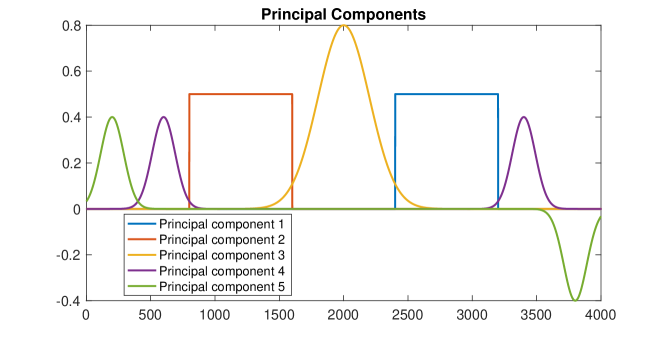
Figure 2: The five principal components used in the synthetic data.

In addition, the matrices corresponding to the random data and the DNA methylation data are shifted and normalized such that their columns have mean zero and standard deviation one. The matrix for the synthetic data is only normalized such that it columns have standard deviation one since the sparsity over the five principal components needs to be preserved.

The parameters $\sigma$, $\nu$, $\mu$, and $N$ in AManPG are set to be $10^{-4}$, $0.5$, $1/(2\|A\|_{2}^{2})$, and $5$ respectively. When the diagonal weight is used, the parameters $\mu$ and $\tau$ are set to be 1 and 0.1, respectively. All the tested algorithms terminate when $\|\eta_{z_{k}}\|_{P}^{2}<\mu n{}{p}10^{-10}$ or the number of iterations exceeds 10000, where $\|\eta_{z_{k}}\|_{P}$ denotes the $\mathrm{F}$-norm for the methods without the diagonal weight and the $W$-norm for the methods with the diagonal weight. The initial guess is constructed from the leading $p$ right singular vectors of the given matrix $A$. Note that the reported computational time of all the algorithms do not include the computational time for the initial iterate.

4.2 Acceleration behavior of AManPG and influence of the safeguard

Here we empirically show that as in the Euclidean case AManPG (with $W=I$ in the Riemannian proximal subproblem) also achieves faster convergence than ManPG, and moreover the safeguard in AManPG is able to stabilize the algorithm while not sacrificing the faster convergence rate. The parameters in ManPG are set to the default values. Figure 3 contains the comparisons in the three different scenarios. Note that AManPG without the safeguard is abbreviated as AManPG w/o SG in the figure, while AManPG simply denotes the method with the safeguard here and later. When both the AManPG methods with and without the safeguard converge, they perform similarly as shown in the left plot. This implies that using safeguard in AManPG does not destroy the efficient performance. In addition, AManPG w/o SG may not converge as shown in the middle and right plots. Therefore, AManPG with the safeguard is preferred since it preserves the global convergence property as ManPG and on the other hand converges faster than ManPG.

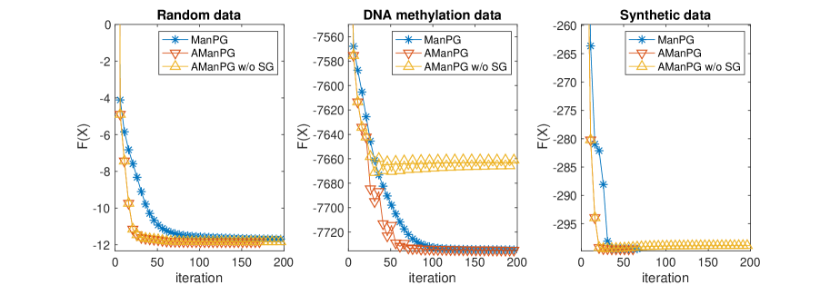
Figure 3: Plots of function values versus iterations for three typical instances with $\mu=1/(1.2\|A\|_{2}^{2})$. Left: Random data, $n=3000$, $m=40$, ${}{p}=4$, $\lambda=2.5$; Middle: DNA methylation data, $n=24589$, $m=113$, ${}{p}=4$, $\lambda=6$; Right: Synthetic data, $n=4000$, $m=400$, ${}{p}=5$, $\lambda=1.5$; The number of restarts in the safeguard in the three tests are 1, 12, and, 3, respectively, from left to right. The values $\|x_{k+1}-x_{k}\|_{F}$ of AManPG w/o SG in the middle and right plots stay above 0.22 and 0.07 respectively, up to 10000 iterations.

4.3 Comparisons with other algorithms

In this section we compare the performance of AManPG and ManPG-Ada with and without diagonal weight. ManPG-Ada is a variant of ManPG which is also introduced in the work of Chen et al. [CMSZ20]. It has been observed in the work [CMSZ20] that AManPG-Ada can achieve faster convergence than ManPG by adaptively adjusting the constant $\mu$ in (3.3). The parameters in ManPG-Ada are set to the default values. Note that the associated algorithms using the diagonal weight computed in the way presented in Section 3.1 are denoted by AManPG-D and ManPG-Ada-D, respectively, while AManPG and ManPG-Ada denote the algorithms without the diagonal weight (i.e., $W=I$ in the Riemannian proximal subproblem). These methods are also compared to SOC (splitting method for orthogonality), as Euclidean space based method introduced in the work of Lai et al.  [LO14]. Since the optimization problem (1.2) can be written as

$$\begin{array}[]{c}\min_{X,Q,P\in\mathbb{R}^{n\times p}}-\operatorname{\mathrm{trace}}(P^{T}A^{T}AP)+\lambda\|Q\|_{1},\\ \hbox{ s.t. $Q=P,X=P,X^{T}X=I_{p}$,}\end{array}$$ (4.3)

the SOC method solves (4.3) by a three-block ADMM:

$$P_{k+1}= \operatorname*{arg\,min}_{P}-\operatorname{\mathrm{trace}}(P^{T}A^{T}AP)+\frac{\beta}{2}\|P-Q_{k}+\Lambda_{k}\|_{\mathrm{F}}^{2}+\frac{\beta}{2}\|P-X_{k}+\Gamma_{k}\|_{\mathrm{F}}^{2},$$ (4.4)

$$Q_{k+1}= \operatorname*{arg\,min}_{Q}\lambda\|Q_{1}\|+\frac{\beta}{2}\|P_{k+1}-Q+\Lambda_{k}\|_{\mathrm{F}}^{2},$$

$$X_{k+1}= \operatorname*{arg\,min}_{X}\frac{\beta}{2}\|P_{k+1}-X+\Gamma_{k}\|_{\mathrm{F}}^{2},\hbox{ s.t. }X^{T}X=I_{p},$$ (4.5)

$$\Lambda_{k+1}= \Lambda_{k}+P_{k+1}-Q_{k+1},$$

$$\Gamma_{k+1}= \Gamma_{k}+P_{k+1}-X_{k+1},$$

where $\beta$ is a constant. Computing $P_{k+1}$ in (4.4) requires to solve a linear system $(\beta I_{n}-A^{T}A)X=B$ for a given matrix $B$. when $m<n$ and $\beta I_{n}-A^{T}A$ is invertible (which holds in our experiments), it is solved by $X=(\beta I_{n}-A^{T}A)^{-1}B=\frac{1}{\beta}\left(B+A^{T}(\beta-AA^{T})^{-1}AB\right)$. The parameter $\beta$ is set to be 2. The SOC method stops when $F(X_{k})<F_{r}+10^{-7}$, where $F_{r}$ is maximum of the function values given by ManPG-Ada, ManPG-Ada-D, AManPG, and AManPG-D. The SOC method has been tested in the work of Chen et al.  [CMSZ20] and it is shown therein that it is the most efficient method among the tested Euclidean space based methods.

Tables 1,  2 and 3 show the performance of the five algorithms with various values of $\lambda$. In the tables, the numbers of iterations, runtime in seconds, final function values, the norms of $\|\eta_{z_{k}}\|_{P}$, sparsity levels and the adjusted variances [ZHT06] are reported. The sparsity level is the portion of entries that are less than $10^{-5}$ in magnitude. The variance in the table refers to the normalized value given by the variance of the sparse PCA solution divided by the maximum variance achieved by the PCA.

Table 1: An average result of 20 random runs for the random data: ${}{p}=4$, $n=3000$ and $m=40$. The subscript $k$ indicates a scale of $10^{k}$.

$\lambda$	Algo	iter	time	$f$	$\|\eta_{z_{k}}\|$	sparsity	variance
2.0	SOC	1894	1.06	$-7.02_{1}$	$\backslash$	0.52	0.84
2.0	ManPG-Ada	359	0.35	$-7.02_{1}$	$5.12_{-4}$	0.52	0.84
2.0	ManPG-Ada-D	335	0.37	$-7.02_{1}$	$5.22_{-4}$	0.52	0.84
2.0	AManPG	128	0.20	$-7.02_{1}$	$4.35_{-4}$	0.52	0.84
2.0	AManPG-D	118	0.21	$-7.02_{1}$	$4.23_{-4}$	0.52	0.84
2.5	SOC	2515	1.43	$-1.44_{1}$	$\backslash$	0.66	0.72
2.5	ManPG-Ada	358	0.36	$-1.44_{1}$	$5.89_{-4}$	0.66	0.72
2.5	ManPG-Ada-D	327	0.39	$-1.44_{1}$	$5.84_{-4}$	0.66	0.72
2.5	AManPG	130	0.22	$-1.44_{1}$	$5.13_{-4}$	0.66	0.72
2.5	AManPG-D	115	0.22	$-1.44_{1}$	$4.99_{-4}$	0.66	0.72
3.0	SOC	3099	1.77	$2.84_{1}$	$\backslash$	0.83	0.48
3.0	ManPG-Ada	389	0.43	$2.84_{1}$	$6.89_{-4}$	0.83	0.48
3.0	ManPG-Ada-D	310	0.43	$2.81_{1}$	$6.96_{-4}$	0.83	0.48
3.0	AManPG	166	0.33	$2.80_{1}$	$6.04_{-4}$	0.83	0.47
3.0	AManPG-D	134	0.31	$2.73_{1}$	$5.65_{-4}$	0.84	0.46

Table 2: The result for the DNA methylation data: ${}{p}=4$, $n=24589$ and $m=113$. The subscript $k$ indicates a scale of $10^{k}$.

$\lambda$	Algo	iter	time	$f$	$\|\eta_{z_{k}}\|$	sparsity	variance
2.0	SOC	5413	134.94	$-9.43_{3}$	$\backslash$	0.10	0.98
2.0	ManPG-Ada	1532	6.43	$-9.43_{3}$	$1.09_{-4}$	0.11	0.98
2.0	ManPG-Ada-D	146	0.87	$-9.43_{3}$	$3.24_{-4}$	0.10	0.98
2.0	AManPG	101	0.81	$-9.43_{3}$	$1.11_{-4}$	0.10	0.98
2.0	AManPG-D	66	0.73	$-9.43_{3}$	$2.61_{-4}$	0.10	0.98
6.0	SOC	2000	51.90	$-7.74_{3}$	$\backslash$	0.29	0.96
6.0	ManPG-Ada	431	2.66	$-7.74_{3}$	$3.08_{-4}$	0.29	0.96
6.0	ManPG-Ada-D	180	1.57	$-7.74_{3}$	$8.14_{-4}$	0.29	0.96
6.0	AManPG	106	1.45	$-7.74_{3}$	$2.68_{-4}$	0.29	0.96
6.0	AManPG-D	56	1.13	$-7.74_{3}$	$5.13_{-4}$	0.29	0.96
10.0	SOC	1516	38.01	$-6.21_{3}$	$\backslash$	0.43	0.94
10.0	ManPG-Ada	144	1.36	$-6.21_{3}$	$4.58_{-4}$	0.43	0.93
10.0	ManPG-Ada-D	50	0.90	$-6.21_{3}$	$1.20_{-3}$	0.43	0.93
10.0	AManPG	66	1.37	$-6.21_{3}$	$2.02_{-4}$	0.43	0.94
10.0	AManPG-D	41	1.30	$-6.21_{3}$	$8.11_{-4}$	0.43	0.93

Table 3: An average result of 20 random runs for the synthetic data: ${}{p}=5$, $n=4000$ and $m=400$. The subscript $k$ indicates a scale of $10^{k}$.

$\lambda$	Algo	iter	time	$f$	$\|\eta_{z_{k}}\|$	sparsity	variance
1.0	SOC	529	9.05	$-3.64_{2}$	$\backslash$	0.61	0.95
1.0	ManPG-Ada	41	0.11	$-3.64_{2}$	$3.17_{-4}$	0.61	0.95
1.0	ManPG-Ada-D	24	0.08	$-3.64_{2}$	$3.97_{-4}$	0.61	0.95
1.0	AManPG	41	0.16	$-3.64_{2}$	$2.09_{-4}$	0.61	0.95
1.0	AManPG-D	31	0.14	$-3.64_{2}$	$2.64_{-4}$	0.61	0.95
1.5	SOC	412	7.29	$-2.99_{2}$	$\backslash$	0.74	0.93
1.5	ManPG-Ada	37	0.10	$-2.99_{2}$	$4.51_{-4}$	0.74	0.93
1.5	ManPG-Ada-D	19	0.08	$-2.99_{2}$	$4.44_{-4}$	0.74	0.93
1.5	AManPG	33	0.15	$-2.99_{2}$	$2.94_{-4}$	0.74	0.93
1.5	AManPG-D	25	0.13	$-2.99_{2}$	$3.59_{-4}$	0.74	0.93
2.0	SOC	375	6.36	$-2.39_{2}$	$\backslash$	0.80	0.91
2.0	ManPG-Ada	46	0.11	$-2.39_{2}$	$5.85_{-4}$	0.80	0.91
2.0	ManPG-Ada-D	17	0.07	$-2.39_{2}$	$6.37_{-4}$	0.80	0.91
2.0	AManPG	33	0.14	$-2.39_{2}$	$3.82_{-4}$	0.80	0.91
2.0	AManPG-D	23	0.12	$-2.39_{2}$	$3.92_{-4}$	0.80	0.91

It can be seen from the tables that the SOC method takes the most computational time to achieve a similar accuracy. In addition, the tables show that AManPG shares the same fast convergence as the Euclidean FISTA method in terms of the number of iterations. Note that the additional computations on the safeguard, the retraction, as well as the inverse of retraction make the per iteration cost of AManPG higher than that of ManPG-Ada. Despite this, due to the significant reduction on the number of iterations, AManPG is still substantially faster than ManPG-Ada in terms of the computational time for the random data and the real DNA data (see Tables 1 and 2). For the synthetic data, Table 3 suggests this problem is relatively easier in the sense that all the algorithms are able to achieve the convergence within a small number of iterations. Thus, the two AManPG algorithms do not exhibit the the computational advantage in terms of the runtime due to the additional costs in each iteration. Moreover, it is evident that using the diagonal weight significantly improves the efficiency of ManPG, ManPG-Ada, and AManPG both in terms of the number of iterations and in terms of the computational time.

4.4 Efficiency for large-scale problems

In this section, the efficiency of the representative method, AManPG-D, is shown for multiple values of $n,m,p$. The values of $\lambda$ are tuned such that the solutions have reasonable sparsities. As shown in Table 4, the trend of the computational time roughly follows the complexity analysis discussed at the end of Section 3.2. Moreover, AManPG-D exhibits high efficiency for the sparse PCA model (1.2) in the sense that it is able to solve the problem with $n=96000,m=1280,p=16$ within half a minute.

Table 4: Performance of AManPG-D with multiple values of $n$, $m,p,\lambda$. An average result of 10 random runs for the random data. The subscript $k$ indicates a scale of $10^{k}$.

$n$	3000	6000	6000	6000	12000	24000	48000	96000
$m$	40	40	80	80	160	320	640	1280
$p$	4	4	4	8	8	8	16	16
$\lambda$	3	3	2	2	1.5	1	0.75	0.5
iter	121	123	139	189	175	146	98	55
time	0.25	0.37	0.46	1.34	2.72	4.40	18.97	29.32
$f$	$2.46_{1}$	$-7.83_{1}$	$1.06_{1}$	$2.70_{1}$	$4.38_{1}$	$1.52_{1}$	$8.02_{1}$	$2.71_{1}$
$\|\eta_{z_{k}}\|$	$5.42_{-4}$	$7.65_{-4}$	$8.07_{-4}$	$1.75_{-3}$	$2.65_{-3}$	$3.88_{-3}$	$1.17_{-2}$	$1.55_{-2}$
sparsity	0.85	0.57	0.76	0.78	0.84	0.77	0.84	0.76
variance	0.43	0.80	0.60	0.58	0.47	0.59	0.48	0.60

4.5 Compare with sparse PCA models in GPower

For the synthetic data, because there exists a ground truth, it is favorable to present the principal components returned by the PCA and that returned by the Riemannian proximal methods for the sparse PCA formulation, see Figure 4 (only the principal components obtained from AManPG-D are reported as a representative). The figure clearly shows that the latter one is more likely to capture the sparse structure of the loading vector.

We have also compared AManPG-D and the GPower with $l_{1}$ and $l_{0}$ norms (designed for a different sparse PCA model, see the work of Journée [JNRS10]) with various sparsity levels. The results are presented in Figures 5, 6 and 7 for the random data, the real DNA data and the synthetic data, respectively. We can see that AManPG-D for (1.2) produces an orthonormal loading matrix while does not lose much variance compared with GPower.

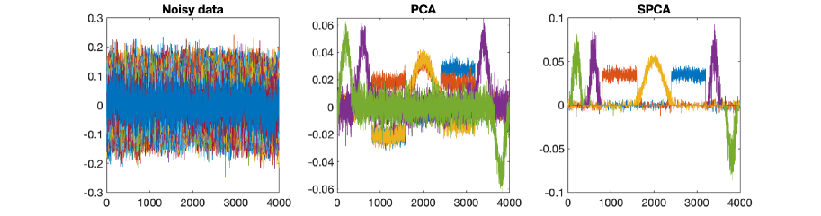
Figure 4: Comparison between the principal components from the PCA and that from the Sparse PCA by AManPG-D with $\lambda=1.5$.

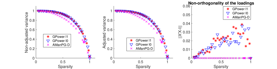
Figure 5: Sparse PCA by AManPG-D and sparse PCA by GPower. Matrix $A\in\mathbb{R}^{3000\times 40}$ is generated randomly. The number of components ${}{p}$ is set to be $4$.

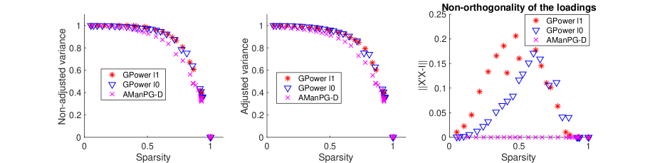
Figure 6: Sparse PCA by AManPG-D and sparse PCA by GPower. Matrix $A\in\mathbb{R}^{24589\times 113}$ is from the DNA methylation data. The number of components ${}{p}$ is set to be $4$.

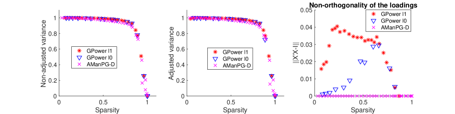
Figure 7: Sparse PCA by AManPG-D and sparse PCA by GPower. Matrix $A\in\mathbb{R}^{4000\times 400}$ is from the synthetic data. The number of components ${}{p}$ is set to be $5$.

5 Conclusion and future directions

In this paper we extend the well-known accelerated first order method FISTA from the Euclidean setting to the Riemannian setting. Moreover, a diagonal preconditioning strategy is also presented which can further accelerate the convergence of the Riemannian proximal gradient methods. Empirical evaluations on the sparse PCA problems have established the computational advantages of the proposed methods. Stationary point convergence of the algorithm has been carefully justified.

There are several lines of research for future directions. In addition to the stationary point analysis, it is also desirable to study the local convergence rate of the Riemannian proximal methods. It is also interesting to develop and study the high order Riemannian methods for the nonsmooth Riemannian optimization problems with the splitting structure. For example, in this paper we only use the diagonal weight to accelerate the convergence of the algorithms for the computational efficiency of the Riemannian proximal subproblem. It is very natural to further consider the Newton type method for this kind of problems. In this case the crux would be to develop efficient algorithms for the scaled proximal mapping on the tangent space. In the work of Li et al. [LST18] a highly efficient semi-smooth Newton augmented Lagrangian method is proposed for the Lasso problem. Due to the similar structures between the Lasso problem and the sparse PCA problem, it is intriguing to see whether or not the method can be extended to solve the sparse PCA problem.

Appendix A Proof of Lemma 3.2

Proof.

We first prove the result of the work [CMSZ20, Lemma 5.1]. Note that the proof is slightly different due to the presence of the weight matrix $W$.

Let $\ell_{\tilde{z}_{i}}(\xi)={\langle\operatorname{\mathrm{grad}}f(\tilde{z}_{i}),\xi_{\tilde{z}_{i}}\rangle}+\frac{1}{2\mu}\|\xi\|_{W_{\tilde{z}_{i}}}^{2}+g(\tilde{z}_{i}+\xi)$. Define functions $\tilde{\ell}_{\tilde{z}_{i}}(\xi)=\langle W_{\tilde{z}_{i}}^{-1/2}\xi_{\tilde{z}_{i}},\xi\rangle+\frac{1}{2\mu}\|\xi\|_{F}^{2}+g(x+W_{\tilde{z}_{i}}^{-1/2}\xi)$ and $\theta(\xi)=W_{\tilde{z}_{i}}^{1/2}\xi$. We have $\ell_{\tilde{z}_{i}}=\tilde{\ell}_{\tilde{z}_{i}}\circ\theta$. By $\frac{1}{\mu}$-strongly convexity of $\tilde{\ell}_{\tilde{z}_{i}}$, we have

$$\tilde{\ell}_{\tilde{z}_{i}}(\hat{\xi})\geq\tilde{\ell}_{\tilde{z}_{i}}({\xi})+{\langle\partial\tilde{\ell}_{\tilde{z}_{i}}({\xi}),\hat{\xi}-\xi\rangle}+\frac{1}{2\mu}\|\hat{\xi}-\xi\|_{F}^{2},\quad\forall\hat{\xi},\xi\in\mathbb{R}^{n\times p},$$

which together with the full rank of $W_{\tilde{z}_{i}}$ yields

$$\ell_{\tilde{z}_{i}}(\hat{\xi})\geq\ell_{\tilde{z}_{i}}(\xi)+{\langle\partial\ell_{\tilde{z}_{i}}(\xi),\hat{\xi}-\xi\rangle}+\frac{1}{2\mu}\|\hat{\xi}-\xi\|_{W_{\tilde{z}_{i}}}^{2}\quad\forall\hat{\xi},\xi\in\mathbb{R}^{n\times p}.$$ (A.1)

By the definition of $\eta_{\tilde{z}_{i}}$ in Step 3 of Algorithm 2 and the optimality condition, we have $0\in\mathrm{P}_{\operatorname{\mathrm{T}}_{\tilde{z}_{i}}}\partial\ell_{\tilde{z}_{i}}(\eta_{\tilde{z}_{i}})$. It follows from (A.1) that

$$\ell_{\tilde{z}_{i}}(0)\geq\ell_{\tilde{z}_{i}}(\eta_{\tilde{z}_{i}})+\frac{1}{2\mu}\|\eta_{\tilde{z}_{i}}\|_{W_{\tilde{z}_{i}}}^{2},$$

which implies

$$g(\tilde{z}_{i})\geq{\langle\operatorname{\mathrm{grad}}f(\tilde{z}_{i}),\eta_{\tilde{z}_{i}}\rangle}+\frac{1}{2\mu}\|\eta_{\tilde{z}_{i}}\|_{W_{\tilde{z}_{i}}}^{2}+g(\tilde{z}_{i}+\eta_{\tilde{z}_{i}})+\frac{1}{2\mu}\|\eta_{\tilde{z}_{i}}\|_{W_{\tilde{z}_{i}}}^{2}.$$

By the convexity of $g$, we have

$$g(\tilde{z}_{i}+\alpha\eta_{\tilde{z}_{i}})-g(\tilde{z}_{i})=g(\alpha(\tilde{z}_{i}+\eta_{\tilde{z}_{i}})+(1-\alpha)\tilde{z}_{i})-g(\tilde{z}_{i})\leq\alpha(g(\tilde{z}_{i}+\eta_{\tilde{z}_{i}})-g(\tilde{z}_{i}))\quad\forall\alpha\in[0,1].$$

Combining the above two inequalities yields

$$\ell_{\tilde{z}_{i}}(\alpha\eta_{\tilde{z}_{i}})-\ell_{\tilde{z}_{i}}(0)\leq\frac{\alpha(\alpha-2)}{2\mu}\|\eta_{\tilde{z}_{i}}\|_{W_{\tilde{z}_{i}}}^{2}\leq\frac{\alpha(\alpha-2){\kappa}}{2\mu}\|\eta_{\tilde{z}_{i}}\|_{F}^{2},$$ (A.2)

where the last inequality follows from Assumption 3.4.

Using (A.2), the first item of Lemma 3.2 can be obtained by exactly following the steps in the work [CMSZ20, Lemma 5.2].

By the definition of $\eta_{\tilde{z}_{i}}$ in Step 3 of Algorithm 2 and the first order optimality condition, we have

$$0\in\frac{1}{\mu}W_{\tilde{z}_{i}}\eta_{\tilde{z}_{i}}+\operatorname{\mathrm{grad}}f(\tilde{z}_{i})+\mathrm{P}_{\operatorname{\mathrm{T}}_{\tilde{z}_{i}}\mathcal{M}}\partial g(\tilde{z}_{i}+\eta_{\tilde{z}_{i}}).$$ (A.3)

If $\eta_{\tilde{z}_{i}}=0$, then it follows from (A.3) that

$$0\in\operatorname{\mathrm{grad}}f(\tilde{z}_{i})+\mathrm{P}_{\operatorname{\mathrm{T}}_{\tilde{z}_{i}}\mathcal{M}}\partial g(\tilde{z}_{i}+\eta_{\tilde{z}_{i}}),$$

which is exactly the first order optimality condition of Problem (1.3). This completes the proof for the second item of Lemma 3.2. ∎

References

- [AMS08] P.-A. Absil, R. Mahony, and R. Sepulchre. Optimization algorithms on matrix manifolds. Princeton University Press, Princeton, NJ, 2008.
- [Bec17] Amir. Beck. First-Order Methods in Optimization. Society for Industrial and Applied Mathematics, Philadelphia, PA, 2017.
- [BFM17] G. C. Bento, O. P. Ferreira, and J. G. Melo. Iteration-complexity of gradient, subgradient and proximal point methods on Riemannian manifolds. Journal of Optimization Theory and Applications, 173(2):548–562, 2017.
- [BL06] J. M. Borwein and A. S. Lewis. Convex Analysis and Nonlinear Optimization: Theory and Examples. Canadian Mathematical Society, 2006.
- [Bou14] N. Boumal. Optimization and estimation on manifolds. PhD thesis, Université catholique de Louvain, 2014.
- [BS72] R. H. Bartels and G. W. Stewart. Solution of the matrix equation . Communications of the ACM, 15(9):820–826, 1972.
- [BST14] J. Bolte, S. Sabach, and M. Teboulle. Proximal alternating linearized minimization for nonconvex and nonsmooth problems. Mathematical Programming (Series A), 146:459–494, 2014.
- [BT09] A. Beck and M. Teboulle. A fast iterative shrinkage-thresholding algorithm for linear inverse problems. SIAM Journal on Imaging Sciences, 2(1):183–202, 2009.
- [Cla90] F. H. Clarke. Optimization and nonsmooth analysis. SIAM, 1990.
- [CMSZ20] Shixiang Chen, Shiqian Ma, Anthony Man-Cho So, and Tong Zhang. Proximal gradient method for nonsmooth optimization over the Stiefel manifold. SIAM Journal on Optimization, 30(1):210–239, 2020.
- [Dar83] John Darzentas. Problem Complexity and Method Efficiency in Optimization. 1983.
- [dBG08] A. d’Aspremont, F. Bach, and L. El Ghaoui. Optimal solutions for sparse principal component analysis. Journal of Machine Learning Research, 9:1269–1294, 2008.
- [dGJL07] A. d’Aspremont, L. E. Ghaoui, M. I. Jordan, and G. R. G. Lanckriet. A direct formulation for sparse PCA using semidefinite programming. SIAM Review, 49(3):434–448, 2007.
- [FO98] O. P. Ferreira and P. R. Oliveira. Subgradient algorithm on Riemannian manifolds. Journal of Optimization Theory and Applications, 97(1):93–104, 1998.
- [FO02] O. P. Ferreira and P. R. Oliveira. Proximal point algorithm on Riemannian manifolds. Optimization, 51(2):257–270, 2002.
- [GH15a] P. Grohs and S. Hosseini. -subgradient algorithms for locally lipschitz functions on Riemannian manifolds. Advances in Computational Mathematics, 2015. DOI: 10.1007/s10444-015-9426-z.
- [GH15b] P. Grohs and S. Hosseini. Nonsmooth trust region algorithms for locally Lipschitz functions on Riemannian manifolds. IMA Journal of Numerical Analysis, 2015. DOI: 10.1093/imanum/drv043.
- [GV96] G. H. Golub and C. F. Van Loan. Matrix computations. Johns Hopkins Studies in the Mathematical Sciences. Johns Hopkins University Press, third edition, 1996.
- [HAGH18] W. Huang, P.-A. Absil, K. A. Gallivan, and P. Hand. ROPTLIB: an object-oriented C++ library for optimization on Riemannian manifolds. ACM Transactions on Mathematical Software, 4(44):43:1–43:21, 2018.
- [HHY18] S. Hosseini, W. Huang, and R. Yousefpour. Line search algorithms for locally Lipschitz functions on Riemannian manifolds. SIAM Journal on Optimization, 28(1):596–619, 2018.
- [HP11] S. Hosseini and M. R. Pouryayevali. Generalized gradient and characterization of epi-Lipschitz sets in Riemannian manifold. Nonlinear Analysis: Theory, Methods & Applications, 72(12):3884–3895, 2011.
- [HU17] S. Hosseini and A. Uschmajew. A Riemannian gradient sampling algorithm for nonsmooth optimization on manifolds. SIAM Journal on Optimization, 27(1):173–189, 2017.
- [Hua13] W. Huang. Optimization algorithms on Riemannian manifolds with applications. PhD thesis, Florida State University, Department of Mathematics, 2013.
- [HW21] W. Huang and K. Wei. Riemannian proximal gradient methods. Mathematical Programming, 2021. doi:10.1007/s10107-021-01632-3.
- [JNRS10] M. Journée, Y. Nesterov, P. Richtárik, and R. Sepulchre. Generalized power method for sparse principal component analysis. Journal of Machine Learning Research, 11:517–553, 2010.
- [JTU03] Ian T. Jolliffe, Nickolay T. Trendafilov, and Mudassir Uddin. A modified principal component technique based on the Lasso. Journal of Computational and Graphical Statistics, 12(3):531–547, 2003.
- [LL15] H. Li and Z. Lin. Accelerated proximal gradient methods for nonconvex programming. In International Conference on Neural Information Processing Systems, 2015.
- [LO14] R. Lai and S. Osher. A splitting method for orthogonality constrained problems. Journal of Scientific Computing, 58(2):431–449, Feb 2014.
- [LSS14] J. Lee, Y. Sun, and M. Saunders. Proximal Newton-type methods for minimizing composite functions. SIAM Journal on Optimization, 24(3):1420–1443, 2014.
- [LST18] X. Li, D. Sun, and K.-C. Toh. A highly efficient semismooth Newton augmented Lagrangian method for solving Lasso problems. SIAM Journal on Optimization, 28(1):433–458, 2018.
- [Mis14] B. Mishra. A Riemannian approach to large-scale constrained least-squares with symmetries. PhD thesis, University of Liege, 2014.
- [Nes83] Y. E. Nesterov. A method for solving the convex programming problem with convergence rate $O(1/k^2)$. Dokl. Akas. Nauk SSSR (In Russian), 269:543–547, 1983.
- [OC15] B. O’Donoghue and E. Candès. Adaptive restart for accelerated gradient schemes. Foundations of Computational Mathematics, 15(3):715–732, 2015.
- [RW98] R. T. Rockafellar and R. J-B Wets. Variational Analysis. Springer-Verlag Berlin Heidelberg, first edition, 1998.
- [SCL+18] K. Sjöstrand, L. Clemmensen, R. Larsen, G. Einarsson, and B. Ersboll. SpaSM: A matlab toolbox for sparse statistical modeling. Journal of Statistical Software, Articles, 84(10):1–37, 2018.
- [SH08] H. Shen and J. Z. Huang. Sparse principal component analysis via regularized low rank matrix approximation. Journal of Multivariate Analysis, 99(6):1015 –1034, 2008.
- [Van10] B. Vandereycken. Riemannian and multilevel optimization for rank-constrained matrix problems (with applications to Lyapunov equations). PhD thesis, Katholieke Universiteit Leuven, 2010.
- [WTH09] D. M. Witten, R. Tibshirani, and T. Hastie. A penalized matrix decomposition, with applications to sparse principal components and canonical correlation analysis. Biostatistics, 10(3):515–534, 2009.
- [XLWZ18] X. Xiao, Y. Li, Z. Wen, and L. Zhang. A regularized semi-smooth Newton method with projection steps for composite convex programs. Journal of Scientific Computing, 76(1):364–389, 2018.
- [YZR14] W. H. Yang, L.-H. Zhang, and Song R. Optimality conditions for the nonlinear programming problems on Riemannian manifolds. Pacific Journal of Optimization, 10(2):415–434, 2014.
- [ZHT06] H. Zou, T. Hastie, and R. Tibshirani. Sparse principal component analysis. Journal of Computational and Graphical Statistics, 15(2):265–286, 2006.
- [ZJN+12] Joanna Zhuang, Allison Jones, Shih-Han Leeand Esther Ng, Heidi Fiegl, Michal Zikan, David Cibula, Alexandra Sargent, Helga B. Salvesen, Ian J. Jacobs, Henry C. Kitchener, Andrew E. Teschendorff, and Martin Widschwendter. The dynamics and prognostic potential of DNA methylation changes at stem cell gene loci in women’s cancer. Plos Genetics, 8(3):e1002517, 2012.
- [ZS16] H. Zhang and S. Sra. First-order methods for geodesically convex optimization. In Conference on Learning Theory, 2016.
- [ZX18] H. Zou and L. Xue. A selective overview of sparse principal component analysis. Proceedings of IEEE, 106(8):1311–1320, 2018.