Higher Secondary Polytopes and Regular Plabic Graphs

Abstract.

Given a configuration $\mathcal{A}$ of $n$ points in $\mathbb{R}^{d-1}$, we introduce the higher secondary polytopes $\widehat{\Upsigma}_{\mathcal{A},1},\dots,\widehat{\Upsigma}_{\mathcal{A},n-d}$, which have the property that $\widehat{\Upsigma}_{\mathcal{A},1}$ agrees with the secondary polytope of Gelfand–Kapranov–Zelevinsky, while the Minkowski sum of these polytopes agrees with Billera–Sturmfels’ fiber zonotope associated with (a lift of) $\mathcal{A}$. In a special case when $d=3$, we refer to our polytopes as higher associahedra. They turn out to be related to the theory of total positivity, specifically, to certain combinatorial objects called plabic graphs, introduced by the second author in his study of the totally positive Grassmannian. We define a subclass of regular plabic graphs and show that they correspond to the vertices of the higher associahedron $\widehat{\Upsigma}_{\mathcal{A},k}$, while square moves connecting them correspond to the edges of $\widehat{\Upsigma}_{\mathcal{A},k}$. Finally we connect our polytopes to soliton graphs, the contour plots of soliton solutions to the KP equation, which were recently studied by Kodama and the third author. In particular, we confirm their conjecture that when the higher times evolve, soliton graphs change according to the moves for plabic graphs.

1. Introduction

Motivated by the study of discriminants, Gelfand, Kapranov, and Zelevinsky [GKZ94] introduced the secondary polytope $\Upsigma_{\mathcal{A}}^{{\operatorname{GKZ}}}$ for a configuration $\mathcal{A}$ of $n$ points in $\mathbb{R}^{d-1}$. Vertices of this remarkable polytope correspond to regular triangulations of the convex hull of $\mathcal{A}$, and its faces correspond to regular polyhedral subdivisions. Billera and Sturmfels [BS92] defined a more general notion of a fiber polytope $\Upsigma^{\operatorname{fib}}(P\overset{\pi}{\to}Q)$ for any linear projection $\pi:P\to Q$ of polytopes. Secondary polytopes are exactly the fiber polytopes in the case when $P$ is a simplex.

In this paper, we extend the notion of a secondary polytope and define the higher secondary polytopes $\widehat{\Upsigma}_{\mathcal{A},1},\dots,\widehat{\Upsigma}_{\mathcal{A},n-d}$ so that $\widehat{\Upsigma}_{\mathcal{A},1}$ coincides with the secondary polytope $\Upsigma_{\mathcal{A}}^{{\operatorname{GKZ}}}$ up to affine translation and dilation. An example of a higher secondary polytope is shown in Figure 1.

Figure 1. The higher secondary polytope $\widehat{\Upsigma}_{\mathcal{A},k}$ for $n=6$, $d=3$, $k=2$, where $\mathcal{A}\subseteq\mathbb{R}^{2}$ is the set of vertices of a generic convex hexagon. Thus $\widehat{\Upsigma}_{\mathcal{A},k}$ is a higher associahedron. The polytope $\widehat{\Upsigma}_{\mathcal{A},k}$ has $32$ vertices, and two points in the interior of $\widehat{\Upsigma}_{\mathcal{A},k}$ (labeled by $b$ and $c$), corresponding to non-regular fine zonotopal tilings, are shown in red. The $34$ points shown in this picture correspond to the $34$ bipartite plabic graphs for $\operatorname{Gr}(3,6)$, and the edges connecting them represent square moves of plabic graphs. See Section 2.3 and Example 7.9 for more details.

Our main motivation for the introduction of polytopes $\widehat{\Upsigma}_{\mathcal{A},k}$ comes from total positivity. [Pos06] constructed a parametrization of the totally positive part $\operatorname{Gr}_{>0}(k,n)$ of the Grassmannian using plabic graphs, which are certain graphs drawn in a disk with vertices colored in two colors. These graphs have interesting combinatorial, algebraic, and geometric features. Remarkably, plabic graphs play a role in several different areas of mathematics and physics: cluster algebras [Sco06], quantum minors [Sco05], soliton solutions of Kadomtsev-Petviashvili (KP) equation [KW11, KW14], scattering amplitudes in $\mathcal{N}=4$ supersymmetric Yang-Mills (SYM) theory [AHBC⁺16], electrical networks [Lam18], the Ising model [GP18], and many other areas.

Plabic graphs are also closely related to polyhedral geometry. There are two variations of plabic graphs: trivalent plabic graphs and bipartite plabic graphs. [Gal18] showed that trivalent plabic graphs can be identified with sections of fine zonotopal tilings of 3-dimensional cyclic zonotopes. A related construction [Pos18] identified trivalent plabic graphs with $\pi$-induced subdivisions for a projection $\pi$ from the hypersimplex $\Delta_{k,n}$ to an $n$-gon. From both points of view, it is natural to define the subclass of regular plabic graphs. Such regular plabic graphs can be explicitly constructed from a vector ${\bm{h}}\in\mathbb{R}^{n}$. Regular trivalent plabic graphs correspond to (1) sections of regular fine zonotopal tilings of a 3-dimensional cyclic zonotope, and (2) vertices of the fiber polytope $\Upsigma^{\operatorname{fib}}(\Delta_{k,n}\overset{\pi}{\to}\text{$n$-gon})$ associated to a projection of a hypersimplex $\Delta_{k,n}$ to a convex $n$-gon.

While regular trivalent plabic graphs correspond to vertices of the fiber polytope $\Upsigma^{\operatorname{fib}}(\Delta_{k,n}\overset{\pi}{\to}\text{$n$-gon})$, regular bipartite plabic graphs also correspond to vertices of certain polytopes, which do not fit into the framework of fiber polytopes. In general, these polytopes are deformations of fiber polytopes, obtained by contracting certain edges of fiber polytopes. These polytopes, whose vertices correspond to regular bipartite plabic graphs, are the higher secondary polytopes $\widehat{\Upsigma}_{\mathcal{A},k}$, where $\mathcal{A}$ is the configuration of vertices of a convex $n$-gon. We call these polytopes higher associahedra, because, for $k=1$, they are the usual secondary polytopes of $n$-gons, which are exactly the celebrated associahedra of Stasheff [Tam51, Sta63].

The study of soliton solutions of the Kadomtsev-Petviashvili (KP) equation also leads to regular trivalent plabic graphs [KW11, KW14, KK18], which were called realizable plabic graphs in [KK18], in the case that $\mathcal{A}=((\kappa_{1},\kappa_{1}^{2}),\dots,(\kappa_{n},\kappa_{n}^{2})).$ To understand a soliton solution $u_{A}(x,y,t)$ of the KP equation coming from a point $A$ in the positive Grassmannian, one fixes the time $t$ and plots the points where $u_{A}(x,y,t)$ has a local maximum. This gives rise to a tropical curve in the $xy$-plane; as soliton solutions model shallow water waves, such as beach waves, this tropical curve shows the positions in the plane where the corresponding wave has a peak. As was shown in [KW11, KW14], this tropical curve is a reduced plabic graph, and hence the Plücker coordinates naturally labeling the regions of the curve form a cluster for the cluster structure on the Grassmannian; the authors moreover speculated in [KW11] that when the time $t$ varies, one observes the face labels of the soliton graph change by cluster transformations, see Figure 2.

Figure 2. A contour plot coming from a point in $\operatorname{Gr}_{>0}(2,4)$ undergoing a cluster mutation as time varies.

We prove this conjecture using the connection between soliton graphs and regular plabic graphs.

Acknowledgements

This project grew out of discussions during the Fall of 2017, while all authors were in residence at the Mathematical Sciences Research Institute in Berkeley, CA. They are grateful to MSRI for providing an ideal work environment. The first author is grateful to Miriam Farber for discussions regarding Figure 1 during the development of [FG18]. The third author would like to thank Yuji Kodama for their joint work on KP solitons, which provided part of the motivation for this project. This work was partially supported by the National Science Foundation under Grant No. DMS-1764370, No. DMS-1440140, No. DMS-1600447, and No. DMS-1854512. Any opinions, findings and conclusions or recommendations expressed in this material are those of the authors and do not necessarily reflect the views of the National Science Foundation.

We now discuss our constructions and results in more detail.

2. Main results

2.1. Background on secondary and fiber polytopes

Let $\mathcal{A}=({\bm{a}}_{1},\dots,{\bm{a}}_{n})$ be a configuration of $n$ points in $\mathbb{R}^{d-1}$, and let $Q\subseteq\mathbb{R}^{d-1}$ be the convex hull of $\mathcal{A}$. We assume that the points in $\mathcal{A}$ affinely span $\mathbb{R}^{d-1}$. An $\mathcal{A}$-triangulation is a polyhedral subdivision of $Q$ formed by simplices of the form $\Delta_{B}:=\mathrm{conv}\{{\bm{a}}_{i}\mid i\in B\}$ for $d$-element subsets $B$ of $[n]:=\{1,\dots,n\}$. We view such simplices $\Delta_{B}$ as labeled by subsets $B$, see Remark 3.7. To every $\mathcal{A}$-triangulation $\tau$, Gelfand–Kapranov–Zelevinsky [GKZ94] associated a point $\mathrm{vert}^{\operatorname{GKZ}}(\tau)\in\mathbb{R}^{n}$ defined by

(2.1) $$\mathrm{vert}^{\operatorname{GKZ}}(\tau):=\sum_{\Delta_{B}\in\tau}\mathrm{Vol}^{d-1}(\Delta_{B})\cdot{\bm{e}}_{B},$$

where $\mathrm{Vol}^{d-1}$ is the usual Euclidean volume in $\mathbb{R}^{d-1}$, ${\bm{e}}_{1},{\bm{e}}_{2},\dots,{\bm{e}}_{n}$ is the standard basis of $\mathbb{R}^{n}$, and we set ${\bm{e}}_{B}:=\sum_{i\in B}{\bm{e}}_{i}$ for $B\subseteq[n]$. The secondary polytope $\Upsigma_{\mathcal{A}}^{{\operatorname{GKZ}}}$ of $\mathcal{A}$ is defined as the convex hull of vectors $\mathrm{vert}^{\operatorname{GKZ}}(\tau)$ where $\tau$ ranges over all $\mathcal{A}$-triangulations. It turns out [GKZ94, Chapter 7, Theorem 1.7] that the vertices of $\Upsigma_{\mathcal{A}}^{{\operatorname{GKZ}}}$ correspond precisely to regular $\mathcal{A}$-triangulations, defined in Section 6.

Billera and Sturmfels [BS92] introduced a more general notion of a fiber polytope $\Upsigma^{\operatorname{fib}}(P\overset{\pi}{\to}Q)$ for any affine projection of polytopes $\pi:P\to Q$, which we review in Section 3.1. If $P:=\Delta^{n-1}=\mathrm{conv}({\bm{e}}_{1},\dots,{\bm{e}}_{n})$ is the standard $(n-1)$-dimensional simplex in $\mathbb{R}^{n}$, $Q:=\mathrm{conv}{\mathcal{A}}$, and $\pi$ is defined by $\pi({\bm{e}}_{i})={\bm{a}}_{i}$ for all $i$, then the fiber polytope $\Upsigma^{\operatorname{fib}}(\Delta^{n-1}\overset{\pi}{\to}Q)$ is a dilation of the secondary polytope $\Upsigma_{\mathcal{A}}^{{\operatorname{GKZ}}}$, see [BS92, Theorem 2.5]. Therefore the vertices of $\Upsigma^{\operatorname{fib}}(\Delta^{n-1}\overset{\pi}{\to}Q)$ correspond to regular $\mathcal{A}$-triangulations.

Another interesting case is when $P=\mbox{\,\mancube\,}_{n}=[0,1]^{n}$ is the standard $n$-cube. Let us denote by $\mathcal{V}:=({\bm{v}}_{1},\dots,{\bm{v}}_{n})$ the lift of $\mathcal{A}$, i.e., the vector configuration in $\mathbb{R}^{d}$ obtained from $\mathcal{A}$ by setting ${\bm{v}}_{i}:=({\bm{a}}_{i},1)\in\mathbb{R}^{d}$ for $i=1,\dots,n$, and let $\mathcal{Z}_{\mathcal{V}}:=\sum_{i=1}^{n}[0,{\bm{v}}_{i}]\subseteq\mathbb{R}^{d}$ be the zonotope associated to $\mathcal{V}$. We have a projection $\mbox{\,\mancube\,}_{n}\overset{\pi}{\to}\mathcal{Z}_{\mathcal{V}}$, defined by $\pi({\bm{e}}_{i})={\bm{v}}_{i}$ for all $i$, and in this case, the fiber polytope $\Upsigma^{\operatorname{fib}}(\mbox{\,\mancube\,}_{n}\overset{\pi}{\to}\mathcal{Z}_{\mathcal{V}})$ is called the fiber zonotope of $\mathcal{Z}_{\mathcal{V}}$. Its vertices correspond to regular fine zonotopal tilings of the zonotope $\mathcal{Z}_{\mathcal{V}}$, discussed below. Restricting this projection map $\pi$ to the hypersimplex $\Delta_{k,n}:=\mbox{\,\mancube\,}_{n}\cap\{{\bm{x}}\in\mathbb{R}^{n}\mid x_{1}+\dots+x_{n}=k\}$, and denoting its image by $Q_{k}:=\pi(\Delta_{k,n})=\mathcal{Z}_{\mathcal{V}}\cap\{{\bm{y}}\in\mathbb{R}^{d}\mid y_{d}=k\}$, we obtain a fiber polytope $\Upsigma^{\operatorname{fib}}(\Delta_{k,n}\overset{\pi}{\to}Q_{k})$ which has recently appeared in the theory of total positivity for Grassmannians [Gal18, Pos18] and was studied further in [OS19].

2.2. Higher secondary polytopes

Given a configuration of $n$ points $\mathcal{A}\subseteq\mathbb{R}^{d-1}$ and its lift $\mathcal{V}\subseteq\mathbb{R}^{d}$ as above, we introduce a family of polytopes $\widehat{\Upsigma}_{\mathcal{A},1},\dots,\widehat{\Upsigma}_{\mathcal{A},n-d}$, called higher secondary polytopes, defined as follows. For a $d$-element subset $B$ of $[n]$, let $\mathrm{Vol}^{d}(\Pi_{B}):=|\det({\bm{v}}_{i})_{i\in B}|$ be the volume of the parallelepiped $\Pi_{B}$ spanned by the vectors $\{{\bm{v}}_{i}\mid i\in B\}$. For a pair of disjoint subsets $A,B$ of $[n]$ such that $|B|=d$ and $\mathrm{Vol}^{d}(\Pi_{B})>0$ (i.e., such that $B$ is a basis of $\mathcal{V}$), define the shifted parallelepiped $\Pi_{A,B}\subseteq\mathcal{Z}_{\mathcal{V}}$ by

$$\Pi_{A,B}:=\sum_{a\in A}{\bm{v}}_{a}+\sum_{b\in B}[0,{\bm{v}}_{b}].$$

Clearly $\mathrm{Vol}^{d}(\Pi_{A,B})=\mathrm{Vol}^{d}(\Pi_{B})$ for any $A$. A fine zonotopal tiling of $\mathcal{Z}_{\mathcal{V}}$ is (roughly speaking) a collection $\mathcal{T}$ of parallelepipeds $\Pi_{A,B}$ that form a polyhedral subdivision of $\mathcal{Z}_{\mathcal{V}}$, see Definition 3.6, and we say that $\mathcal{T}$ is regular if it can be obtained as a projection of the upper boundary of a $(d+1)$-dimensional zonotope onto $\mathcal{Z}_{\mathcal{V}}$, see Definition 6.3.

Definition 2.1.

For a fine zonotopal tiling $\mathcal{T}$ of $\mathcal{Z}_{\mathcal{V}}$ and $k\in\mathbb{Z}$, we introduce a vector

(2.2) $$\widehat{\mathrm{vert}}_{k}(\mathcal{T}):=\sum_{\begin{subarray}{c}\Pi_{A,B}\in\mathcal{T}\\ |A|=k\end{subarray}}\mathrm{Vol}^{d}(\Pi_{B})\cdot{\bm{e}}_{A}\in\mathbb{R}^{n}.$$

It is clear that $\widehat{\mathrm{vert}}_{k}(\mathcal{T})=0$ if $k\notin[n-d]$. For $k\in[n-d]$, the higher secondary polytope $\widehat{\Upsigma}_{\mathcal{A},k}$ is defined by

$$\widehat{\Upsigma}_{\mathcal{A},k}:=\mathrm{conv}\left\{\widehat{\mathrm{vert}}_{k}(\mathcal{T})\;\middle|\;\text{$\mathcal{T}$ is a fine \emph{regular} zonotopal tiling of $\mathcal{Z}_{\mathcal{V}}$}\right\}.$$

We expect that the word regular can be omitted from the above definition, see 6.6. As we will see in Proposition 6.7, for each $k\in[n-d]$, the polytope $\widehat{\Upsigma}_{\mathcal{A},k}$ has dimension $n-d$. An example of a higher secondary polytope is shown in Figure 1.

For simplicity, we formulate the following result modulo affine translation. A more precise formulation will be given in (6.3). For polytopes $P,P^{\prime}\subseteq\mathbb{R}^{m}$, we write $P\stackrel{{\scriptstyle\mathclap{\mbox{\scalebox{0.6}{shift}}}}}{{=\joinrel=}}P^{\prime}$ if $P=P^{\prime}+{\bm{\gamma}}$ for some $\bm{\gamma}\in\mathbb{R}^{m}$.

Theorem 2.2.

Let $\mathcal{A}\subseteq\mathbb{R}^{d-1}$ be a point configuration. Recall that $Q=\mathrm{conv}\mathcal{A}$, $\mathcal{V}\subseteq\mathbb{R}^{d}$ is the lift of $\mathcal{A}$, $\mathcal{Z}_{\mathcal{V}}$ is the zonotope of $\mathcal{V}$, and $Q_{k}=\mathcal{Z}_{\mathcal{V}}\cap\{{\bm{y}}\in\mathbb{R}^{d}\mid y_{d}=k\}$ is the $k$-th section of $\mathcal{Z}_{\mathcal{V}}$. Then we have the following.

1. $\Upsigma_{\mathcal{A}}^{{\operatorname{GKZ}}}\stackrel{{\scriptstyle\mathclap{\mbox{\scalebox{0.6}{shift}}}}}{{=\joinrel=}}\frac{1}{(d-1)!}\widehat{\Upsigma}_{\mathcal{A},1}$, equivalently, $\Upsigma^{\operatorname{fib}}(\Delta^{n-1}\overset{\pi}{\to}Q)\stackrel{{\scriptstyle\mathclap{\mbox{\scalebox{0.6}{shift}}}}}{{=\joinrel=}}\frac{1}{d!\mathrm{Vol}^{d-1}(Q)}\widehat{\Upsigma}_{\mathcal{A},1}$.

2. $\Upsigma^{\operatorname{fib}}(\mbox{\,\mancube\,}_{n}\overset{\pi}{\to}\mathcal{Z}_{\mathcal{V}})\stackrel{{\scriptstyle\mathclap{\mbox{\scalebox{0.6}{shift}}}}}{{=\joinrel=}}\frac{1}{\mathrm{Vol}^{d}(\mathcal{Z}_{\mathcal{V}})}\left(\widehat{\Upsigma}_{\mathcal{A},1}+\cdots+\widehat{\Upsigma}_{\mathcal{A},n-d}\right)$.

3. $\Upsigma^{\operatorname{fib}}(\Delta_{k,n}\overset{\pi}{\to}Q_{k})\stackrel{{\scriptstyle\mathclap{\mbox{\scalebox{0.6}{shift}}}}}{{=\joinrel=}}\frac{1}{\mathrm{Vol}^{d-1}(Q_{k})}\left(p_{0,d}\widehat{\Upsigma}_{\mathcal{A},k}+p_{1,d}\widehat{\Upsigma}_{\mathcal{A},k-1}+\dots+p_{d-1,d}\widehat{\Upsigma}_{\mathcal{A},k-d+1}\right)$ for all $k\in[n-1]$, where $p_{r,d}$ is the probability that a random permutation in $S_{d}$ has $r$ descents.

4. Duality: $\widehat{\Upsigma}_{\mathcal{A},k}\stackrel{{\scriptstyle\mathclap{\mbox{\scalebox{0.6}{shift}}}}}{{=\joinrel=}}-\widehat{\Upsigma}_{\mathcal{A},n-d-k+1}$ for all $k\in[n-d]$.

   Here we assume that $\widehat{\Upsigma}_{\mathcal{A},k}$ is a single point if $k\notin[n-d]$. The volume forms $\mathrm{Vol}^{d}$ and $\mathrm{Vol}^{d-1}$ on $\mathbb{R}^{d}$ are scaled so that $\mathrm{Vol}^{d}([0,1]^{d})=\mathrm{Vol}^{d-1}([0,1]^{d-1}\times\{y_{d}\})=1$ for any $y_{d}\in\mathbb{R}$. The numbers $p_{r,d}$ are given by the formula $p_{r,d}=\frac{\genfrac{\langle}{\rangle}{0.0pt}{}{d}{r}}{d!}$, where $\genfrac{\langle}{\rangle}{0.0pt}{}{d}{r}$ is the Eulerian number, i.e., the number of permutations of $1,2,\dots,d$ with exactly $r$ descents.

   Remark 2.3.

   2.2 is not an obvious consequence of the definitions: it says that $\Upsigma_{\mathcal{A}}^{{\operatorname{GKZ}}}$ (defined by (2.1)) is the convex hull of points

   (2.3) $$\frac{1}{(d-1)!}\sum_{\begin{subarray}{c}\Pi_{A,B}\in\mathcal{T}\\ |A|=1\end{subarray}}\mathrm{Vol}^{d}(\Pi_{B})\cdot{\bm{e}}_{A}$$

   for all regular fine zonotopal tilings $\mathcal{T}$ of $\mathcal{Z}_{\mathcal{V}}$. The formulae (2.1) and (2.3) are quite different: we have ${\bm{e}}_{B}$ in (2.1) as opposed to ${\bm{e}}_{A}$ in (2.3), and we have $|A|=0$ in (2.1) as opposed to $|A|=1$ in (2.3).

   On the other hand, it is easy to see from the definitions that the last higher secondary polytope $\widehat{\Upsigma}_{\mathcal{A},n-d}$ satisfies $\Upsigma_{\mathcal{A}}^{{\operatorname{GKZ}}}\stackrel{{\scriptstyle\mathclap{\mbox{\scalebox{0.6}{shift}}}}}{{=\joinrel=}}-\frac{1}{(d-1)!}\widehat{\Upsigma}_{\mathcal{A},n-d}$. Thus 2.2 follows from 2.2.

   Remark 2.4.

   The polytope $\widehat{\Upsigma}_{\mathcal{A},k}$ in Figure 1 is centrally symmetric, in agreement with 2.2: we have $k=2=n-k-d+1$, thus $\widehat{\Upsigma}_{\mathcal{A},k}\stackrel{{\scriptstyle\mathclap{\mbox{\scalebox{0.6}{shift}}}}}{{=\joinrel=}}-\widehat{\Upsigma}_{\mathcal{A},k}$.

   Example 2.5.

   Let $d=1$ and let $\mathcal{A}$ be the configuration of $n$ points ${\bm{a}}_{1}=\cdots={\bm{a}}_{n}=0\in\mathbb{R}^{0}$. Then $\mathcal{V}$ is the configuration of $n$ vectors ${\bm{v}}_{1}=\dots={\bm{v}}_{n}=(1)\in\mathbb{R}^{1}$, and the zonotope $\mathcal{Z}_{\mathcal{V}}$ is the interval $[0,n]\subseteq\mathbb{R}^{1}$. There are $n!$ fine zonotopal tilings of $\mathcal{Z}_{\mathcal{V}}$ (see Definition 3.6), in bijection with the permutations $w\in S_{n}$. More specifically, for each $w\in S_{n}$, we have the following fine zonotopal tiling $\mathcal{T}_{w}$ of $\mathcal{Z}_{\mathcal{V}}$:

   $$\mathcal{T}_{w}:=\left\{\Pi_{\emptyset,\{w_{1}\}},\Pi_{\{w_{1}\},\{w_{2}\}},\dots,\Pi_{\{w_{1},\dots,w_{n-1}\},\{w_{n}\}}\right\}.$$

   Even though geometrically the tilings $\mathcal{T}_{w}$ are the same for all $w\in S_{n}$, we treat them as different tilings because we take into account the labels of the tiles, see Remark 3.7. We have $\widehat{\mathrm{vert}}_{k}(\mathcal{T}_{w})={\bm{e}}_{\{w_{1},\dots,w_{k}\}}$, thus $\widehat{\Upsigma}_{\mathcal{A},k}$ is the hypersimplex $\Delta_{k,n}$. It is straightforward to see from the definitions (cf. [BS92, Example 5.4] or [Zie95, Example 9.8]) that $n\cdot\Upsigma^{\operatorname{fib}}(\mbox{\,\mancube\,}_{n}\overset{\pi}{\to}\mathcal{Z}_{\mathcal{V}})$ is the permutohedron $\operatorname{Perm}_{n}:=\mathrm{conv}\{(w_{1},\dots,w_{n})\mid w\in S_{n}\}$. Thus 2.2 recovers the following well known decomposition [Pos09, Section 16] (implicit in [GS87]) of the permutohedron as a Minkowski sum of hypersimplices:

   $$\operatorname{Perm}_{n}=\Delta_{1,n}+\Delta_{2,n}+\dots+\Delta_{n-1,n}.$$

   More generally, one can consider the case where $\mathcal{V}$ is a cyclic vector configuration $C(n,d)$, i.e., is given by ${\bm{v}}_{i}=(u_{i}^{d-1},\dots,u_{i},1)$ for $i\in[n]$ and $0<u_{1}<u_{2}<\dots<u_{n}\in\mathbb{R}$. Thus Example 2.5 corresponds to the case $d=1$. If $d=2$, then the zonotope $\mathcal{Z}_{\mathcal{V}}$ is a $2n$-gon, and fine zonotopal tilings are exactly the rhombus tilings of the $2n$-gon. They correspond to commutation classes of reduced decompositions of the longest permutation $w_{0}\in S_{n}$ [Eln97]. It would be interesting to understand the structure of the associated higher secondary polytopes in more detail.

   Remark 2.6.

   For a cyclic vector configuration $C(n,d)$, Ziegler [Zie93] identified the fine zonotopal tilings of the cyclic zonotope $\mathcal{Z}_{\mathcal{V}}$ with elements of Manin-Shekhtman’s higher Bruhat order $B(n,d)$ [MS89], also studied by Voevodsky and Kapranov [VK91]. Note that $B(n,1)$ coincides with the weak Bruhat order on permutations, corresponding to the case $d=1$ in Example 2.5.

   We next proceed to the case $d=3$.

   2.3. Higher associahedra and plabic graphs

   Our main motivating example is the case when $\widehat{\Upsigma}_{\mathcal{A},k}$ is a higher associahedron, that is, when $d=3$ and $\mathcal{A}$ is the configuration of vertices of a convex $n$-gon in $\mathbb{R}^{2}$. For example, one could take the points in $\mathcal{A}$ lying on a parabola, in which case the lift $\mathcal{V}$ of $\mathcal{A}$ is a cyclic vector configuration $C(n,3)$. It turns out that the combinatorics of higher associahedra is directly related to bipartite plabic graphs that were introduced in [Pos06] in the study of the totally nonnegative Grassmannian $\operatorname{Gr}_{\geq 0}(k,n)$.

   A plabic graph is a planar graph embedded in a disk such that every boundary vertex has degree $1$ and every interior vertex is colored either black or white. A plabic graph is called trivalent if every interior vertex has degree $3$, and it is called bipartite if no two interior vertices of the same color are connected by an edge. Note that taking a trivalent plabic graph $G$ and contracting all edges between interior vertices of the same color produces a bipartite plabic graph denoted $G^{{\operatorname{bip}}}$.

   There is a special class of $(k,n)$-plabic graphs (cf. Definition 7.1), that were used in [Pos06] to parametrize the top-dimensional cell of $\operatorname{Gr}_{\geq 0}(k,n)$. Each $(k,n)$-plabic graph has $n$ boundary vertices and $k(n-k)+1$ faces, and its face labels (cf. Definition 7.2) form a cluster in the cluster algebra structure on the coordinate ring of the Grassmannian [Sco06].

   Figure 3. A plabic graph and its bipartite version.

   (M1)	(M2)	(M3)

   Figure 4. Moves on plabic graphs.

   Given a plabic graph, one can apply certain moves to it, as shown in Figure 4. Any two trivalent $(k,n)$-plabic graphs can be connected using moves (M1)–(M3), see [Pos06, Theorem 13.4]. Since applying the moves (M1) and (M3) to $G$ does not change its bipartite version $G^{{\operatorname{bip}}}$, it follows that any two bipartite $(k,n)$-plabic graphs can be connected using only the square move (M2). For example, there are $34$ bipartite $(3,6)$-plabic graphs corresponding to the $34$ points in Figure 1 (including the two points labeled by $b$ and $c$), and square moves between them correspond to the edges in Figure 1.

   Building on the work of Oh–Postnikov–Speyer [OPS15], it was shown in [Gal18] that trivalent $(k,n)$-plabic graphs are exactly the planar duals of the horizontal sections of fine zonotopal tilings of the zonotope $\mathcal{Z}_{\mathcal{V}}$ (where $\mathcal{V}\subseteq\mathbb{R}^{3}$ is the lift of $\mathcal{A}$ as above), see Theorem 7.3. It was later observed in [Pos18] that trivalent $(k,n)$-plabic graphs correspond to $\pi$-induced subdivisions for the map $\pi:\Delta_{k,n}\to Q_{k}$.

   We say that a trivalent $(k,n)$-plabic graph $G$ is $\mathcal{A}$-regular if it is the planar dual of a horizontal section of some regular fine zonotopal tiling of $\mathcal{Z}_{\mathcal{V}}$, or equivalently, if it corresponds to a regular $\pi$-induced subdivision of $Q_{k}$. We say that a bipartite $(k,n)$-plabic graph $G^{\prime}$ is $\mathcal{A}$-regular if it equals to $G^{{\operatorname{bip}}}$ for some $\mathcal{A}$-regular trivalent $(k,n)$-plabic graph $G$. For example, if $\mathcal{A}$ is the set of vertices of a generic hexagon, then there are $32$ $\mathcal{A}$-regular bipartite $(3,6)$-plabic graphs, corresponding to the $32$ vertices of the polytope shown in Figure 1. See Example 7.9 for more details.

   Theorem 2.7.

   Let $d=3$ and $\mathcal{A}$ be the configuration of vertices of a convex $n$-gon. Then:

   1. For each $k\in[n-3]$, the vertices of $\widehat{\Upsigma}_{\mathcal{A},k}$ correspond to $\mathcal{A}$-regular bipartite $(k+1,n)$-plabic graphs, and the square moves connecting them correspond to the edges of $\widehat{\Upsigma}_{\mathcal{A},k}$.

   2. For each $k\in[n-1]$, the vertices of $\widehat{\Upsigma}_{\mathcal{A},k}+\widehat{\Upsigma}_{\mathcal{A},k-1}+\widehat{\Upsigma}_{\mathcal{A},k-2}$ (equivalently, of $\Upsigma^{\operatorname{fib}}(\Delta_{k,n}\overset{\pi}{\to}Q_{k})$) correspond to $\mathcal{A}$-regular trivalent $(k,n)$-plabic graphs, and the moves (M1)–(M3) connecting them correspond to the edges of $\widehat{\Upsigma}_{\mathcal{A},k}+\widehat{\Upsigma}_{\mathcal{A},k-1}+\widehat{\Upsigma}_{\mathcal{A},k-2}$.

   Example 2.8.

   The number of bipartite $(2,n)$-plabic graphs equals to the number of trivalent $(1,n)$-plabic graphs, and is given by the Catalan number $C_{n-2}$, where $C_{m}:=\frac{1}{m+1}{2m\choose m}$. In both cases, all such plabic graphs are regular, and the corresponding polytope is $\widehat{\Upsigma}_{\mathcal{A},1}$ which by 2.2 is a realization of the associahedron.

   Figure 5. A trivalent, bipartite $(4,8)$-plabic graph which admits only $4$ square moves, superimposed onto its dual plabic tiling. This plabic graph is not $\mathcal{A}$-regular for any $\mathcal{A}$, see Example 2.9.

   Example 2.9.

   Since $\widehat{\Upsigma}_{\mathcal{A},k}$ has dimension $n-d$ by Proposition 6.7, it follows from (iv) that every $\mathcal{A}$-regular bipartite $(k,n)$-plabic graph admits at least $n-d=n-3$ square moves. Figure 5 contains a (both trivalent and bipartite) $(4,8)$-plabic graph that admits only $4$ square moves, and therefore is not $\mathcal{A}$-regular for any $\mathcal{A}$. This plabic graph contains as a subgraph another plabic graph known in physics as the “four-mass box”, see [AHBC⁺16, Section 11.1].

   An example of a trivalent $(9,18)$-plabic graph that is not $\mathcal{A}$-regular for any $\mathcal{A}$ was constructed in [KK18, Section 6].

   Let us say that the diameter of a polytope is the maximal graph distance between its vertices in its $1$-skeleton. It would be interesting to find the diameter of a higher associahedron $\widehat{\Upsigma}_{\mathcal{A},k}$, which equals the maximal square move distance between two $\mathcal{A}$-regular plabic graphs. Finding the diameter of the usual associahedron $\widehat{\Upsigma}_{\mathcal{A},1}$ is a well-studied problem: answering a question of Sleator–Tarjan–Thurston [STT88], Pournin [Pou14] showed that it equals $2n-10$ for all $n>12$. The following conjecture is due to Miriam Farber.

   Conjecture 2.10 ([Far]).

   Let $n=2k$. Then the diameter of the higher associahedron $\widehat{\Upsigma}_{\mathcal{A},k-1}$ equals $\frac{1}{2}k(k-1)^{2}$. More generally, for any bipartite $(k,2k)$-plabic graph $G$, the minimal number of square moves needed to connect $G$ with $G^{\operatorname{op}}$ equals $\frac{1}{2}k(k-1)^{2}$, where $G^{\operatorname{op}}$ is obtained from $G$ by a $180^{\circ}$ rotation followed by changing the colors of all vertices.

   An example for $k=3$ is shown in Figure 1. The diameter of this polytope is equal to $\frac{1}{2}k(k-1)^{2}=6$, and moreover the graph distance between any vertex and its antipodal vertex is also equal to $6$.

   It was shown in [BW18, Section 6] that for certain bipartite $(k,2k)$-plabic graphs $G$ (coming from double wiring diagrams of [FZ99]), the square move distance between $G$ and $G^{\operatorname{op}}$ is at least $\frac{1}{2}k(k-1)^{2}$, giving a lower bound on the diameter of $\widehat{\Upsigma}_{\mathcal{A},k-1}$ in 2.10. See [BW19] for related results.

   2.4. Vertices, edges, and deformations

   For simplicity, we assume here that $\mathcal{A}$ is a generic point configuration in $\mathbb{R}^{d-1}$. The extension of the results in this subsection to arbitrary point configurations will be given in Section 6.3.

   It is well known (cf. Lemma 6.5) that any two regular fine zonotopal tilings of $\mathcal{Z}_{\mathcal{V}}$ can be related to each other by a sequence of flips. A flip is an elementary transformation of a zonotopal tiling: if $\mathcal{V}^{\prime}$ consists of $d+1$ vectors that span $\mathbb{R}^{d}$ then $\mathcal{Z}_{\mathcal{V}^{\prime}}$ admits precisely two fine zonotopal tilings. For general vector configurations $\mathcal{V}$, applying a flip $F=(\mathcal{T}\to\mathcal{T}^{\prime})$ to a fine zonotopal tiling $\mathcal{T}$ of $\mathcal{Z}_{\mathcal{V}}$ amounts to finding a shifted copy of a fine zonotopal tiling of $\mathcal{Z}_{\mathcal{V}^{\prime}}$ for some $\mathcal{V}^{\prime}\subseteq\mathcal{V}$ of size $d+1$, and replacing it with the other fine zonotopal tiling of $\mathcal{Z}_{\mathcal{V}^{\prime}}$, which produces another fine zonotopal tiling $\mathcal{T}^{\prime}$ of $\mathcal{Z}_{\mathcal{V}}$, see Figure 8 (left). Flips can occur at different levels: if the above copy of $\mathcal{Z}_{\mathcal{V}^{\prime}}$ is shifted by ${\bm{y}}\in\mathbb{R}^{d}$, then the last coordinate $y_{d}$ of ${\bm{y}}$ belongs to $\{0,1,\dots,n-d-1\}$, and we define the level of the flip $F$ to be $\mathrm{level}(F):=y_{d}+1$. See Definition 5.8 and Example 5.10.

   Since flips of regular fine zonotopal tilings correspond to the edges of the fiber zonotope $\Upsigma^{\operatorname{fib}}(\mbox{\,\mancube\,}_{n}\overset{\pi}{\to}\mathcal{Z}_{\mathcal{V}})$, we define the level of an edge of $\Upsigma^{\operatorname{fib}}(\mbox{\,\mancube\,}_{n}\overset{\pi}{\to}\mathcal{Z}_{\mathcal{V}})$ to be the level of the corresponding flip.

   Let us say that a polytope $P$ is a parallel deformation of another polytope $P^{\prime}$ if the normal fan of $P$ is a coarsening of the normal fan of $P^{\prime}$, see e.g. [PRW08, Theorem 15.3] and  [ACEP19, Section 2.2]. Roughly speaking, $P$ is a parallel deformation of $P^{\prime}$ if $P$ is obtained from $P^{\prime}$ by moving its faces while preserving their direction. During this process, every edge of $P^{\prime}$ stays parallel to itself but gets rescaled by some nonnegative real number.

   We say that two fine zonotopal tilings $\mathcal{T}$ and $\mathcal{T}^{\prime}$ of $\mathcal{Z}_{\mathcal{V}}$ are $k$-equivalent if they can be connected by flips $F$ such that $\mathrm{level}(F)\neq k$. Similarly, we say that two flips $F=(\mathcal{T}_{1}\to\mathcal{T}_{2})$ and $F^{\prime}=(\mathcal{T}^{\prime}_{1}\to\mathcal{T}^{\prime}_{2})$ of level $k$ are $k$-equivalent if $\mathcal{T}_{1}$ is $k$-equivalent to $\mathcal{T}^{\prime}_{1}$ and $\mathcal{T}_{2}$ is $k$-equivalent to $\mathcal{T}^{\prime}_{2}$.

   Proposition 2.11.

   Let $\mathcal{A}$ be a generic configuration of $n$ points in $\mathbb{R}^{d-1}$, and let $k\in[n-d]$.

   1. The vertices of the higher secondary polytope $\widehat{\Upsigma}_{\mathcal{A},k}$ are in bijection with $k$-equivalence classes of regular fine zonotopal tilings of $\mathcal{Z}_{\mathcal{V}}$.

   2. The edges of $\widehat{\Upsigma}_{\mathcal{A},k}$ correspond to $k$-equivalence classes of flips of level $k$.

   3. For any nonnegative real numbers $x_{1},\dots,x_{n-d}$, the Minkowski sum

      $$\frac{1}{\mathrm{Vol}^{d}(\mathcal{Z}_{\mathcal{V}})}\left(x_{1}\widehat{\Upsigma}_{\mathcal{A},1}+\dots+x_{n-d}\widehat{\Upsigma}_{\mathcal{A},n-d}\right)$$

      is a parallel deformation of the fiber zonotope $\Upsigma^{\operatorname{fib}}(\mbox{\,\mancube\,}_{n}\overset{\pi}{\to}\mathcal{Z}_{\mathcal{V}})$, where edges of level $k$ are rescaled by $x_{k}$ for all $k=1,\dots,n-d$.

   2.5. Soliton graphs

   Finally we give applications of our previous results to the soliton graphs [KW11, KW14, KK18] associated to the Kadomtsev-Petviashvili (KP) equation. To understand a soliton solution $u_{A}(x,y,t)$ of the KP equation coming from a point $A$ in the positive Grassmannian, one fixes the time $t$ and plots the points where $u_{A}(x,y,t)$ has a local maximum. This gives rise to a tropical curve in the $xy$-plane. By [KW11, KW14], this tropical curve is a reduced plabic graph, and as discussed in [KK18, Section 2.3], it comes from a regular subdivision of a three-dimensional cyclic zonotope; we give a precise statement in Corollary 8.6. We then apply some of our previous results to classify the soliton graphs coming from the positive Grassmannian when the time parameter $t$ tends to $\pm\infty$, and to show that generically, when the higher time parameters evolve, the face labels of soliton graphs change via the square moves (cluster transformations) on plabic graphs.

   3. Fiber polytopes and zonotopal tilings

   We give further background on fiber polytopes of [BS92] and discuss several specializations of their construction. More details can be found in [BS92], [GKZ94, Chapter 7], and [Zie95, Lecture 9].

   3.1. Fiber polytopes

   Let $P\subseteq\mathbb{R}^{n}$ be a polytope, and let $\pi:P\to Q$ be a linear projection of polytopes. We denote by $\{{\bm{p}}_{i}\}_{i\in[m]}$ the vertex set of $P$ (for some $m\geq 1$). For $i\in[m]$, let ${\bm{q}}_{i}:=\pi({\bm{p}}_{i})$, and let $\mathcal{A}:=\{{\bm{q}}_{i}\}_{i\in[m]}$ be the associated point configuration. The fiber polytope $\Upsigma^{\operatorname{fib}}(P\overset{\pi}{\to}Q)$ is defined as the Minkowski integral Σ^fib(Pπ→Q):= 1Vol(Q)∫_x∈Q (π^-1(x)∩P)  dx. Here $\mathrm{Vol}$ denotes the $\dim(Q)$-dimensional volume form on the affine span of $Q$, and the Minkowski integral can be understood in several ways, for example, as the set of points $\int_{{\bm{x}}\in Q}\gamma({\bm{x}})\,d{\bm{x}}\in\mathbb{R}^{n},$ where $\gamma:Q\to P$ runs over all sections of $\pi$ [BS92, BS94].

   However, instead of working with the Minkowski integral, we will use the following description of $\Upsigma^{\operatorname{fib}}(P\overset{\pi}{\to}Q)$ as a convex hull of points. Recall that an $\mathcal{A}$-triangulation $\tau=\{\Delta_{B}\}$ is a triangulation of $Q$ into simplices $\Delta_{B}:=\mathrm{conv}\{{\bm{q}}_{i}\mid i\in B\}$, where $B\subseteq[m]$ is a $(\dim(Q)+1)$-element subset.

   Proposition 3.1 ([BS92, Corollary 2.6]).

   The fiber polytope $\Upsigma^{\operatorname{fib}}(P\overset{\pi}{\to}Q)$ equals the convex hull

   $$\Upsigma^{\operatorname{fib}}(P\overset{\pi}{\to}Q)=\mathrm{conv}\{\mathrm{vert}^{\operatorname{fib}}(\tau)\mid\tau\text{ is an $\mathcal{A}$-triangulation}\},\quad\text{where}$$

   (3.1) $$\mathrm{vert}^{\operatorname{fib}}(\tau):=\frac{1}{(\dim(Q)+1)\mathrm{Vol}(Q)}\sum_{\Delta_{B}\in\tau}\left(\mathrm{Vol}(\Delta_{B})\cdot\sum_{i\in B}{\bm{p}}_{i}\right)\in\mathbb{R}^{n}.$$

   Definition 3.2 ([Zie95, Definition 9.1]).

   Let $\pi:P\to Q$ be a projection of polytopes as above. A $\pi$-induced subdivision of $Q$ is a collection $\mathcal{T}$ of faces of $P$ such that

   • the images $\{\pi(F)\mid F\in\mathcal{T}\}$ form a polyhedral subdivision of $Q$;

   • for any $F,F^{\prime}\in\mathcal{T}$ such that $\pi(F)\subseteq\pi(F^{\prime})$, we have $F=F^{\prime}\cap\pi^{-1}(\pi(F))$.

   A $\pi$-induced subdivision $\mathcal{T}$ is called fine if all of its faces have dimension at most $\dim(Q)$.

   Definition 3.3.

   For a polytope $P\subseteq\mathbb{R}^{n}$ and a vector ${\bm{h}}\in\mathbb{R}^{n}$, let $(P)^{\bm{h}}$ denote the face of $P$ that maximizes the scalar product with ${\bm{h}}$. Every vector ${\bm{h}}\in\mathbb{R}^{n}$ gives rise to a $\pi$-induced subdivision $\mathcal{T}_{\bm{h}}$ of $Q$ obtained as follows: for each point ${\bm{q}}\in Q$, consider the preimage $P\cap\pi^{-1}({\bm{q}})$ of ${\bm{q}}$ under $\pi$, and let $P_{{\bm{q}},{\bm{h}}}$ be the unique minimal by inclusion face of $P$ that contains $(P\cap\pi^{-1}({\bm{q}}))^{\bm{h}}$. The subdivision $\mathcal{T}_{\bm{h}}$ consists of the faces $P_{{\bm{q}},{\bm{h}}}$ for all ${\bm{q}}\in Q$. A $\pi$-induced subdivision $\mathcal{T}$ of $Q$ is called regular if it equals $\mathcal{T}_{\bm{h}}$ for some ${\bm{h}}\in\mathbb{R}^{n}$.

   Our notion of a regular $\pi$-induced subdivision coincides with the notion of a $\pi$-coherent subdivision from [BS92, Section 1] and [Zie95, Definition 9.2].

   It turns out (see the paragraph before [BS92, Corollary 2.7]) that if $\mathcal{T}$ is a fine $\pi$-induced subdivision then the vector $\mathrm{vert}^{\operatorname{fib}}(\tau)$ is the same for any triangulation $\tau$ of $\mathcal{T}$. We denote this vector by $\mathrm{vert}^{\operatorname{fib}}(\mathcal{T})$.

   Corollary 3.4 ([BS92, Corollary 2.7]).

   The fiber polytope $\Upsigma^{\operatorname{fib}}(P\overset{\pi}{\to}Q)$ equals the convex hull

   (3.2) $$\Upsigma^{\operatorname{fib}}(P\overset{\pi}{\to}Q) =\mathrm{conv}\{\mathrm{vert}^{\operatorname{fib}}(\mathcal{T})\mid\mathcal{T}\text{ is a fine $\pi$-induced subdivision of $Q$}\}.$$

   The vertices of $$\Upsigma^{\operatorname{fib}}(P\to Q) \mathrm{vert}^{\operatorname{fib}}(\mathcal{T}) \mathcal{T} \pi Q$$ are the vectors , where ranges over all regular fine -induced subdivisions of , and in particular,

   (3.3) $$\Upsigma^{\operatorname{fib}}(P\overset{\pi}{\to}Q) =\mathrm{conv}\{\mathrm{vert}^{\operatorname{fib}}(\mathcal{T})\mid\mathcal{T}\text{ is a \emph{regular} fine $\pi$-induced subdivision of $Q$}\}.$$

   We now specialize this construction to the case where $P$ is either a cube or a (hyper)simplex. In these cases, regular fine $\pi$-induced subdivisions recover well-studied objects such as regular triangulations and regular fine zonotopal tilings. We discuss them briefly here, and in more detail in Section 6. In what follows, we will repeatedly use the following notation.

   Notation 3.5.

   Let $\mathcal{A}=({\bm{a}}_{1},\dots,{\bm{a}}_{n})$ be a point configuration in $\mathbb{R}^{d-1}$ which affinely spans $\mathbb{R}^{d-1}$. Let $\mathcal{V}:=({\bm{v}}_{1},\dots,{\bm{v}}_{n})$ be the lift of $\mathcal{A}$, thus ${\bm{v}}_{i}:=({\bm{a}}_{i},1)\in\mathbb{R}^{d}$ for $i=1,\dots,n$. Then the endpoints of the vectors in $\mathcal{V}$ belong to $H_{1}$, where the hyperplane $H_{k}$ is defined by $H_{k}:=\{{\bm{y}}\in\mathbb{R}^{d}\mid y_{d}=k\}$ in $\mathbb{R}^{d}$. The zonotope $\mathcal{Z}_{\mathcal{V}}$ is defined as the Minkowski sum of line segments: Z_V:=∑_i=1^n [0,v_i] ⊆R^d. We also let $Q_{k}:=\mathcal{Z}_{\mathcal{V}}\cap H_{k}\subseteq\mathbb{R}^{d}$. Let $\pi$ be the projection $\pi:\mathbb{R}^{n}\to\mathbb{R}^{d}$ defined by $\pi({\bm{e}}_{i})={\bm{v}}_{i}$ for all $i$, where ${\bm{e}}_{1},\dots,{\bm{e}}_{n}$ is the standard basis in $\mathbb{R}^{n}$.

   3.2. Fiber polytopes for projections of a cube: fiber zonotopes

   Let $P=\mbox{\,\mancube\,}_{n}:=[0,1]^{n}=\sum_{i=1}^{n}[0,{\bm{e}}_{i}]\subseteq\mathbb{R}^{n}$ be the standard $n$-dimensional cube. We have a linear projection $\pi:\mbox{\,\mancube\,}_{n}\to\mathcal{Z}_{\mathcal{V}}$ given by $\pi({\bm{e}}_{i})={\bm{v}}_{i}$, for $i\in[n]$. The fiber zonotope of $\mathcal{Z}_{\mathcal{V}}$ is the fiber polytope $\Upsigma^{\operatorname{fib}}(\mbox{\,\mancube\,}_{n}\overset{\pi}{\to}\mathcal{Z}_{\mathcal{V}})$.

   Recall that for $A\subseteq[n]$, we set ${\bm{e}}_{A}:=\sum_{i\in A}{\bm{e}}_{i}$. Faces $\square_{A,B}$ of the $n$-cube $\mbox{\,\mancube\,}_{n}$ are labeled by pairs $(A,B)$ of disjoint subsets $A$ and $B$ of $[n]$. They are given by

   $$\square_{A,B}:={\bm{e}}_{A}+\sum_{b\in B}[0,{\bm{e}}_{b}]=\{(x_{1},\dots,x_{n})\in\mbox{\,\mancube\,}_{n}\mid x_{a}=1\textrm{ for }a\in A,\textrm{ and }x_{c}=0\textrm{ for }c\in[n]\setminus(A\sqcup B)\}.$$

   Definition 3.6.

   A fine zonotopal tiling $\mathcal{T}$ of $\mathcal{Z}_{\mathcal{V}}$ is a collection of $d$-dimensional faces $\square_{A,B}$ of the $n$-cube such that

   1. The images $\Pi_{A,B}:=\pi(\square_{A,B})$, for all $\square_{A,B}\in\mathcal{T}$, are $d$-dimensional parallelepipeds that form a polyhedral subdivision of the zonotope $\mathcal{Z}_{\mathcal{V}}$.

   2. For any two faces $\square_{A_{1},B_{1}},\,\square_{A_{2},B_{2}}\in\mathcal{T}$, we have π(□_A_1,B_1∩□_A_2,B_2) = Π_A_1,B_1 ∩Π_A_2,B_2.

   From our definition, it is clear that each fine zonotopal tiling is a fine $\pi$-induced subdivision. We say that a fine zonotopal tiling is regular if the corresponding fine $\pi$-induced subdivision is regular. See Section 6.1 for several alternative definitions.

   Remark 3.7.

   We refer to the $d$-parallelepipeds $\Pi_{A,B}=\pi(\square_{A,B})$ as (labeled) tiles. It may happen that for two different pairs $(A_{1},B_{1})$ and $(A_{2},B_{2})$, the two tiles $\Pi_{A_{1},B_{1}}$ and $\Pi_{A_{2},B_{2}}$ coincide as subsets of $\mathbb{R}^{d}$. However, we regard them as different labeled tiles, because they are labeled by different pairs. We will identify a fine zonotopal tiling $\mathcal{T}$ with the collection of such labeled tiles $\Pi_{A,B}$.

   The fiber zonotope of $\mathcal{Z}_{\mathcal{V}}$ can be described explicitly as follows.

   Proposition 3.8.

   Let $\mathcal{V}\subseteq\mathbb{R}^{d}$ be as in 3.5. The fiber zonotope $\Upsigma^{\operatorname{fib}}(\mbox{\,\mancube\,}_{n}\overset{\pi}{\to}\mathcal{Z}_{\mathcal{V}})$ equals the convex hull

   (3.4) $$\Upsigma^{\operatorname{fib}}(\mbox{\,\mancube\,}_{n}\overset{\pi}{\to}\mathcal{Z}_{\mathcal{V}}) =\mathrm{conv}\{\mathrm{vert}^{\operatorname{fib}}(\mathcal{T})\mid\mathcal{T}\text{ is a fine zonotopal tiling of $\mathcal{Z}_{\mathcal{V}}$}\},\quad\text{and}$$

   (3.5) $$\mathrm{vert}^{\operatorname{fib}}(\mathcal{T}) =\frac{1}{\mathrm{Vol}(\mathcal{Z}_{\mathcal{V}})}\sum_{\Pi_{A,B}\in\mathcal{T}}\mathrm{Vol}^{d}(\Pi_{B})\cdot\left({\bm{e}}_{A}+\frac{1}{2}{\bm{e}}_{B}\right).$$

   Proof.

   We use (3.1), and let $\tau$ be a triangulation of a fixed tile $\Pi_{A,B}$ of $\mathcal{T}$. More specifically, we use Stanley’s triangulation [Sta77] of $\mbox{\,\mancube\,}_{d}$ into $d!$ equal-volume simplices $\nabla_{w}$ labeled by permutations $w\in S_{d}$:

   (3.6) $$\nabla_{w}:=\{(y_{1},\dots,y_{d})\in[0,1]^{d}\ \mid\ 0<y_{w_{1}}<\dots<y_{w_{d}}<1\}.$$

   This gives rise to a triangulation $\tau$ of $\Pi_{A,B}$ into $d!$ simplices, each of volume $\frac{\mathrm{Vol}^{d}(\Pi_{B})}{d!}$. By symmetry, we know that the combined contribution of these simplices to (3.1) has the form $x\cdot{\bm{e}}_{A}+y\cdot{\bm{e}}_{B}$ for some $x,y\in\mathbb{R}$. Each simplex $\nabla_{w}$ contributes $\frac{\mathrm{Vol}^{d}(\Pi_{B})}{d!\mathrm{Vol}(\mathcal{Z}_{\mathcal{V}})}{\bm{e}}_{A}+{\bm{u}}(w)$ for some ${\bm{u}}(w)\in\mathbb{R}^{n}$. Let $\bar{w}\in S_{d}$ be the permutation given by $\bar{w}_{i}=w_{d+1-i}$ for all $i\in[d]$. It is easy to see that ${\bm{u}}(w)+{\bm{u}}(\bar{w})=\frac{\mathrm{Vol}^{d}(\Pi_{B})}{d!\mathrm{Vol}(\mathcal{Z}_{\mathcal{V}})}{\bm{e}}_{B}$, thus $x=\frac{\mathrm{Vol}^{d}(\Pi_{B})}{\mathrm{Vol}(\mathcal{Z}_{\mathcal{V}})}$ and $y=\frac{\mathrm{Vol}^{d}(\Pi_{B})}{2\mathrm{Vol}(\mathcal{Z}_{\mathcal{V}})}$. ∎

   3.3. Fiber polytopes for projections of a simplex: secondary polytopes.

   Let $\mathcal{A}$ and $\mathcal{V}$ be as in 3.5. Let $P=\Delta^{n-1}=\mathrm{conv}({\bm{e}}_{1},\dots,{\bm{e}}_{n})$ be the standard $(n-1)$-dimensional simplex in $\mathbb{R}^{n}$, and $\pi:P\to Q:=\mathrm{conv}{\mathcal{A}}$ the projection defined by $\pi({\bm{e}}_{i})={\bm{a}}_{i}$ for all $i$.

   Definition 3.9 ([GKZ94, Definition 1.6]).

   The secondary polytope $\Upsigma_{\mathcal{A}}^{{\operatorname{GKZ}}}$ is defined as the convex hull

   (3.7) $$\Upsigma_{\mathcal{A}}^{{\operatorname{GKZ}}} :=\mathrm{conv}\{\mathrm{vert}^{\operatorname{GKZ}}(\tau)\mid\tau\text{ is an $\mathcal{A}$-triangulation}\},\quad\text{where}$$

   (3.8) $$\mathrm{vert}^{\operatorname{GKZ}}(\tau) :=\sum_{\Delta_{B}\in\tau}\mathrm{Vol}^{d-1}(\Delta_{B})\cdot{\bm{e}}_{B}.$$

   The relationship between the polytopes $\Upsigma_{\mathcal{A}}^{{\operatorname{GKZ}}}$ and $\Upsigma^{\operatorname{fib}}(\Delta^{n-1}\overset{\pi}{\to}Q)$ is given in [BS92, Theorem 2.5]:

   $$\Upsigma^{\operatorname{fib}}(\Delta^{n-1}\overset{\pi}{\to}Q)=\frac{1}{d\cdot\mathrm{Vol}^{d-1}(Q)}\Upsigma_{\mathcal{A}}^{{\operatorname{GKZ}}}.$$

   Remark 3.10.

   Every fine zonotopal tiling $\mathcal{T}$ gives rise to an $\mathcal{A}$-triangulation $\tau:=\{\Delta_{B}\mid\Pi_{\emptyset,B}\in\mathcal{T}\}$, in which case we denote $\mathrm{vert}^{\operatorname{GKZ}}(\mathcal{T}):=\mathrm{vert}^{\operatorname{GKZ}}(\tau)$.

   3.4. Fiber polytopes for projections of a hypersimplex: hypersecondary polytopes.

   Recall the definitions of $\mathcal{V}$, $\mathcal{Z}_{\mathcal{V}}$, $\pi$, $H_{k}$, and $Q_{k}$ from 3.5. Also recall that $\Delta_{k,n}=\mbox{\,\mancube\,}_{n}\cap\{{\bm{x}}\in\mathbb{R}^{n}\mid x_{1}+\dots+x_{n}=k\}$. Note that if $k=1$, then $\Delta_{1,n}=\Delta^{n-1}$. We discuss the fiber polytope $\Upsigma^{\operatorname{fib}}(\Delta_{k,n}\overset{\pi}{\to}Q_{k})$. Such polytopes have been recently studied in [OS19] under the name hypersecondary polytopes (not to be confused with higher secondary polytopes $\widehat{\Upsigma}_{\mathcal{A},k}$ introduced in this paper).

   For integers $r$ and $d$, the Eulerian number $\genfrac{\langle}{\rangle}{0.0pt}{}{d}{r}$ is defined as the number of permutations in $S_{d}$ with $r$ descents, where a descent of a permutation $w$ is a position $i$ such that $w_{i}>w_{i+1}$ (thus $\genfrac{\langle}{\rangle}{0.0pt}{}{d}{r}$ is zero if $r\notin[0,d-1]$). For example, we have $\genfrac{\langle}{\rangle}{0.0pt}{}{3}{0}=1$, $\genfrac{\langle}{\rangle}{0.0pt}{}{3}{1}=4$, $\genfrac{\langle}{\rangle}{0.0pt}{}{3}{2}=1$.

   Lemma 3.11.

   Let $\mathcal{T}$ be a fine zonotopal tiling of $\mathcal{Z}_{\mathcal{V}}\subseteq\mathbb{R}^{d}$. Then for all $r\in[d-1]$ and $\Pi_{A,B}\in\mathcal{T}$, we have

   (3.9) $$\mathrm{Vol}^{d-1}(\Pi_{A,B}\cap H_{|A|+r})=\frac{\genfrac{\langle}{\rangle}{0.0pt}{}{d-1}{r-1}}{(d-1)!}\mathrm{Vol}^{d}(\Pi_{B}).$$

   Proof.

   We have $\Pi_{A,B}=\pi(\mbox{\,\mancube\,}_{A,B})$ for $A,B$ disjoint subsets and $|B|=d$. The intersection $\Pi_{A,B}\cap H_{|A|+r}$ is the image of a hypersimplex $\Delta_{r,d}\subseteq\square_{A,B}\cong\mbox{\,\mancube\,}_{d}$ under $\pi$. By [Sta77], $\Delta_{r,d}$ can be triangulated into $\genfrac{\langle}{\rangle}{0.0pt}{}{d-1}{r-1}$ equal-volume simplices, and the image of each of these simplices under $\pi$ has volume $\frac{\mathrm{Vol}^{d}(\Pi_{B})}{(d-1)!}$. ∎

   Proposition 3.12.

   The fiber polytope $\Upsigma^{\operatorname{fib}}(\Delta_{k,n}\overset{\pi}{\to}Q_{k})$ equals the convex hull

   (3.10) $$\Upsigma^{\operatorname{fib}}(\Delta_{k,n}\overset{\pi}{\to}Q_{k}) =\mathrm{conv}\{\mathrm{vert}^{\operatorname{fib}}_{k}(\mathcal{T})\mid\mathcal{T}\text{ is a fine zonotopal tiling of $\mathcal{Z}_{\mathcal{V}}$}\},\quad\text{where}$$

   (3.11) $$\mathrm{vert}^{\operatorname{fib}}_{k}(\mathcal{T}) :=\frac{1}{d!\cdot\mathrm{Vol}^{d-1}(Q_{k})}\sum_{r=1}^{d-1}\sum_{\begin{subarray}{c}\Pi_{A,B}\in\mathcal{T}\\ |A|=k-r\end{subarray}}\mathrm{Vol}^{d}(\Pi_{B})\cdot\genfrac{\langle}{\rangle}{0.0pt}{}{d-1}{r-1}\cdot(d\cdot{\bm{e}}_{A}+r\cdot{\bm{e}}_{B}).$$

   Proof.

   Let $\mathcal{T}$ be a fine zonotopal tiling of $\mathcal{Z}_{\mathcal{V}}$. Then $\mathcal{T}\cap H_{k}:=\{\Pi_{A,B}\cap H_{k}\mid\Pi_{A,B}\in\mathcal{T}\}$ is a fine $\pi$-induced subdivision for the projection $\Delta_{k,n}\overset{\pi}{\to}Q_{k}$. A tile $\Pi_{A,B}\in\mathcal{T}$ has a full-dimensional intersection with $H_{k}$ whenever $|A|+r=k$ for some $r\in[d-1]$. In this case, $\Pi_{A,B}\cap H_{k}$ can be triangulated into $\genfrac{\langle}{\rangle}{0.0pt}{}{d-1}{r-1}$ simplices as in the proof of Lemma 3.11. Proceeding as in the proof of Proposition 3.8, we find that the combined contribution of these simplices to (3.1) is precisely $\frac{\mathrm{Vol}^{d}(\Pi_{B})}{d!\cdot\mathrm{Vol}^{d-1}(Q_{k})}(d\cdot{\bm{e}}_{A}+r\cdot{\bm{e}}_{B})$. Thus we have shown that $\Upsigma^{\operatorname{fib}}(\Delta_{k,n}\overset{\pi}{\to}Q_{k})$ contains the right hand side of (3.10).

   On the other hand, by (3.3), it is enough to consider only regular fine $\pi$-induced subdivisions, and every such subdivision clearly arises as $\mathcal{T}\cap H_{k}$ for some regular fine zonotopal tiling $\mathcal{T}$. This shows that the right hand side of (3.10) contains $\Upsigma^{\operatorname{fib}}(\Delta_{k,n}\overset{\pi}{\to}Q_{k})$. ∎

   Example 3.13.

   For $d=2$, (3.11) becomes

   (3.12) $$\mathrm{vert}^{\operatorname{fib}}_{k}(\mathcal{T}):=\frac{1}{\mathrm{Vol}^{d-1}(Q_{k})}\sum_{\begin{subarray}{c}\Pi_{A,B}\in\mathcal{T}\\ |A|=k-1\end{subarray}}\mathrm{Vol}^{d}(\Pi_{B})\cdot\left({\bm{e}}_{A}+\frac{1}{2}{\bm{e}}_{B}\right).$$

   Example 3.14.

   Substituting $k=1$ into (3.11) and comparing the result with (3.8), we find

   (3.13) $$\mathrm{vert}^{\operatorname{GKZ}}(\mathcal{T}) =d\cdot\mathrm{Vol}^{d-1}(Q_{1})\cdot\mathrm{vert}^{\operatorname{fib}}_{1}(\mathcal{T})\quad\text{and}\quad\Upsigma_{\mathcal{A}}^{{\operatorname{GKZ}}}=d\cdot\mathrm{Vol}^{d-1}(Q_{1})\cdot\Upsigma^{\operatorname{fib}}(\Delta_{1,n}\overset{\pi}{\to}Q_{1}),$$

   in agreement with (3.3).

   4. Vertices of fiber polytopes and vertices of higher secondary polytopes

   Recall the definitions of $\mathcal{V}\subseteq\mathbb{R}^{d},\mathcal{Z}_{\mathcal{V}},H_{k}$, $Q_{k}$, and $\pi$ from 3.5. Also recall that $\Delta_{k,n}=\mbox{\,\mancube\,}_{n}\cap\{{\bm{x}}\in\mathbb{R}^{n}\mid x_{1}+\dots+x_{n}=k\}$. In this section, we prove Theorem 4.6, which gives a duality identity, and expresses the vertices of fiber polytopes $\Upsigma^{\operatorname{fib}}(\mbox{\,\mancube\,}_{n}\overset{\pi}{\to}\mathcal{Z}_{\mathcal{V}})$, $\Upsigma_{\mathcal{A}}^{{\operatorname{GKZ}}}$, and $\Upsigma^{\operatorname{fib}}(\Delta_{k,n}\overset{\pi}{\to}Q_{k})$ as linear combinations of the vectors $\widehat{\mathrm{vert}}_{k}(\mathcal{T})$ defined in (2.2). This will constitute one of the main steps in the proof of Theorem 2.2, which we give in Section 6.2.

   We start by giving a refinement of the simple fact that for any fine zonotopal tiling $\mathcal{T}$, the sum $\sum_{\Pi_{A,B}\in\mathcal{T}}\mathrm{Vol}^{d}(\Pi_{B})$ equals $\mathrm{Vol}^{d}(\mathcal{Z}_{\mathcal{V}})$, and therefore does not depend on $\mathcal{T}$. For $k\in[n-1]$, we let

   (4.1) $$\beta_{k}:=\mathrm{Vol}^{d-1}(Q_{k}),$$

   and we set $\beta_{k}:=0$ for $k\notin[n-1]$.

   Proposition 4.1.

   Fix a vector configuration $\mathcal{V}\subseteq\mathbb{R}^{d}$ as in 3.5. For each $k\in[0,n-d]$, there exists a number $\gamma_{k}^{d}(\mathcal{V})=\gamma_{k}(\mathcal{V})\in\mathbb{R}_{>0}$ such that for any fine zonotopal tiling $\mathcal{T}$, we have

   (4.2) $$\gamma_{k}^{d}(\mathcal{V})=\gamma_{k}(\mathcal{V})=\sum_{\begin{subarray}{c}\Pi_{A,B}\in\mathcal{T}\\ |A|=k\end{subarray}}\mathrm{Vol}^{d}(\Pi_{B}).$$

   Proof.

   Let us temporarily denote

   $$\tilde{\gamma}_{k}(\mathcal{T},\mathcal{V}):=\sum_{\begin{subarray}{c}\Pi_{A,B}\in\mathcal{T}\\ |A|=k\end{subarray}}\mathrm{Vol}^{d}(\Pi_{B})$$

   for all $k\in\mathbb{Z}$. Then $\beta_{k}=\mathrm{Vol}^{d-1}(Q_{k})=\mathrm{Vol}^{d-1}(\mathcal{Z}_{\mathcal{V}}\cap H_{k})=\sum_{\Pi_{A,B}\in\mathcal{T}}\mathrm{Vol}^{d-1}(\Pi_{A,B}\cap H_{k}).$ Applying (3.9), we find that $\beta_{k}=\sum_{r=1}^{d-1}\tilde{\gamma}_{k-r}(\mathcal{T},\mathcal{V})\cdot\frac{\genfrac{\langle}{\rangle}{0.0pt}{}{d-1}{r-1}}{(d-1)!}$. Since the coefficient of $\tilde{\gamma}_{k-1}$ in the right hand side is equal to $\frac{1}{(d-1)!}$, the numbers $\tilde{\gamma}_{k}(\mathcal{T},\mathcal{V})$ can be expressed in terms of the $\beta_{r}$’s by induction for $k=0,1,\dots,n-d$. Explicitly, let $A_{d-1}(x):=\sum_{r=0}^{d-2}\genfrac{\langle}{\rangle}{0.0pt}{}{d-1}{r}x^{r}$ be the Eulerian polynomial, and let $c_{0},c_{1},\dots\in\mathbb{Z}$ be defined by $\frac{1}{A_{d-1}(x)}=c_{0}+c_{1}x+c_{2}x^{2}+\dots$ (thus $c_{0}=1$). Then we have $\tilde{\gamma}_{k}(\mathcal{T},\mathcal{V})=c_{0}\beta_{k+1}+c_{1}\beta_{k}+c_{2}\beta_{k-1}+\dots+c_{k+1}\beta_{0}$ for all $k\in[0,n-d]$. It is clear that $\tilde{\gamma}_{k}(\mathcal{T},\mathcal{V})$ does not depend on $\mathcal{T}$, and so we can refer to it as $\gamma_{k}(\mathcal{V})$. ∎

   Example 4.2.

   For $d=2,3,4$, we have respectively

   (4.3) $$\gamma_{k}^{2}(\mathcal{V}) =\beta_{k+1},$$

   (4.4) $$\gamma_{k}^{3}(\mathcal{V}) =\beta_{k+1}-\beta_{k}+\dots+(-1)^{k+1}\beta_{0},$$

   (4.5) $$\gamma_{k}^{4}(\mathcal{V}) =\beta_{k+1}-4\beta_{k}+15\beta_{k-1}-56\beta_{k-2}+\dots,$$

   where the coefficients of (4.5) form the sequence A125905 in the OEIS [OEI].

   For $i\in[n]$, let $\mathcal{V}-i$ denote the vector configuration in $\mathbb{R}^{d}$ obtained from $\mathcal{V}$ by omitting ${\bm{v}}_{i}$. For each $k\in[0,n-d]$, we introduce a vector $\bm{\delta}(k,\mathcal{V})\in\mathbb{R}^{n}$ whose $i$th coordinate equals

   (4.6) $$\delta_{i}(k,\mathcal{V}):=\gamma_{k}(\mathcal{V})-\gamma_{k}(\mathcal{V}-i)\quad\text{for all $i\in[n]$}.$$

   For $k\notin[0,n-d]$, we set $\gamma_{k}(\mathcal{V}):=0\in\mathbb{R}$ and $\bm{\delta}(k,\mathcal{V}):=0\in\mathbb{R}^{n}$. Recall that the vectors of $\mathcal{V}$ are assumed to linearly span $\mathbb{R}^{d}$. If the vectors of $\mathcal{V}-i$ all belong to a lower-dimensional subspace of $\mathbb{R}^{d}$, we say that $i$ is a coloop and set $\gamma_{k}(\mathcal{V}-i):=0$ for all $k$.

   The following result will be useful in the proof of Theorem 4.6.

   Proposition 4.3.

   For all $k\in[0,n-d]$, we have

   (4.7) $$\sum_{\begin{subarray}{c}\Pi_{A,B}\in\mathcal{T}\\ |A|=k\end{subarray}}\mathrm{Vol}^{d}(\Pi_{B})\cdot({\bm{e}}_{A}+{\bm{e}}_{B})=\sum_{\begin{subarray}{c}\Pi_{A,B}\in\mathcal{T}\\ |A|=k+1\end{subarray}}\mathrm{Vol}^{d}(\Pi_{B})\cdot{\bm{e}}_{A}+\bm{\delta}(k,\mathcal{V}).$$

   Proof.

   Fix $i\in[n]$. We first show that

   (4.8) $$\sum_{\begin{subarray}{c}\Pi_{A,B}\in\mathcal{T}\\ |A|=k+1,\ i\in A\end{subarray}}\mathrm{Vol}^{d}(\Pi_{B})+\sum_{\begin{subarray}{c}\Pi_{A,B}\in\mathcal{T}\\ |A|=k,\ i\notin A\sqcup B\end{subarray}}\mathrm{Vol}^{d}(\Pi_{B})=\gamma_{k}(\mathcal{V}-i).$$

   Assume that $i$ is a coloop, which means that the vectors in $\mathcal{V}-i$ do not linearly span $\mathbb{R}^{d}$, in which case the right hand side of (4.8) is zero. On the other hand, for each tile $\Pi_{A,B}\in\mathcal{T}$, we must have $i\in B$, which shows that the left hand side of (4.8) is also zero. Assume now that $i$ is not a coloop. Then each fine zonotopal tiling $\mathcal{T}$ of $\mathcal{Z}_{\mathcal{V}}$ gives rise to a fine zonotopal tiling $\mathcal{T}-i$ of $\mathcal{Z}_{\mathcal{V}-i}$ defined by

   $$\mathcal{T}-i:=\{\Pi_{A\setminus\{i\},B}\mid\Pi_{A,B}\in\mathcal{T},\ i\in A\}\sqcup\{\Pi_{A,B}\mid\Pi_{A,B}\in\mathcal{T},\ i\notin A\sqcup B\}.$$

   Using this observation, we see that (4.8) follows from the definition (4.2) of $\gamma_{k}(\mathcal{V}-i)$. For the example in Figure 6, for $k=1$, the left hand side of (4.8) is equal to $3+2$ as shown in Figure 6 (middle) while the right hand side of (4.8) is equal to $5$ as shown in Figure 6 (right).

   Figure 6. Deleting ${\bm{v}}_{i}$ from $\mathcal{V}$ and its effect on a tiling $\mathcal{T}$, see (4.8).

   To prove (4.7), it is enough to verify what it says for the $i$th coordinate, which is:

   (4.9) $$\sum_{\begin{subarray}{c}\Pi_{A,B}\in\mathcal{T}\\ |A|=k,\ i\in A\sqcup B\end{subarray}}\mathrm{Vol}^{d}(\Pi_{B})=\sum_{\begin{subarray}{c}\Pi_{A,B}\in\mathcal{T}\\ |A|=k+1,\ i\in A\end{subarray}}\mathrm{Vol}^{d}(\Pi_{B})+\delta_{i}(k,\mathcal{V}).$$

   Adding $\displaystyle\sum_{\begin{subarray}{c}\Pi_{A,B}\in\mathcal{T}\\ |A|=k,\ i\notin A\sqcup B\end{subarray}}\mathrm{Vol}^{d}(\Pi_{B})$ to both sides of (4.9) and applying (4.8) gives $\gamma_{k}(\mathcal{V})=\gamma_{k}(\mathcal{V}-i)+\delta_{i}(k,\mathcal{V})$, which is precisely the definition (4.6) of $\bm{\delta}(k,\mathcal{V})$. ∎

   Corollary 4.4.

   Recall the definition of $\widehat{\mathrm{vert}}_{k}(\mathcal{T})$ from (2.2). Let $K\subseteq\mathbb{Z}$ and choose some numbers $x_{k},y_{k}\in\mathbb{R}$ for each $k\in K$. Then

   (4.10) $$\sum_{\begin{subarray}{c}\Pi_{A,B}\in\mathcal{T}\\ k:=|A|\in K\end{subarray}}\mathrm{Vol}^{d}(\Pi_{B})\cdot(x_{k}{\bm{e}}_{A}+y_{k}{\bm{e}}_{B})=\sum_{k\in K}\left((x_{k}-y_{k})\widehat{\mathrm{vert}}_{k}(\mathcal{T})+y_{k}(\widehat{\mathrm{vert}}_{k+1}(\mathcal{T})+\bm{\delta}(k,\mathcal{V}))\right).$$

   Proof.

   This follows by replacing $x_{k}{\bm{e}}_{A}+y_{k}{\bm{e}}_{B}$ on the left hand side of (4.10) with $(x_{k}-y_{k}){\bm{e}}_{A}+y_{k}({\bm{e}}_{A}+{\bm{e}}_{B})$, and applying Proposition 4.3. ∎

   Definition 4.5.

   Given two disjoint sets $A,B\subseteq[n]$, let $C:=[n]\setminus(A\sqcup B)$, and denote $\Pi_{A,B,C}:=\Pi_{A,B}$. For each zonotopal tiling $\mathcal{T}$ of $\mathcal{Z}_{\mathcal{V}}$ there exists “the opposite” zonotopal tiling $\mathcal{T}^{\operatorname{op}}$ of $\mathcal{Z}_{\mathcal{V}}$ given by $\mathcal{T}^{\operatorname{op}}:=\{\Pi_{C,B,A}\mid\Pi_{A,B,C}\in\mathcal{T}\}$, see Figure 7.

   Theorem 4.6.

   Recall the definitions of $\mathrm{vert}^{\operatorname{fib}}(\mathcal{T})$, $\mathrm{vert}^{\operatorname{fib}}_{k}(\mathcal{T})$, and $\mathrm{vert}^{\operatorname{GKZ}}(\mathcal{T})$ from (3.5), (3.11), and Remark 3.10. We have

   (4.11) $$\mathrm{vert}^{\operatorname{fib}}(\mathcal{T})=\frac{1}{\mathrm{Vol}^{d}(\mathcal{Z}_{\mathcal{V}})}\left(\sum_{k=1}^{n-d}\widehat{\mathrm{vert}}_{k}(\mathcal{T})+\frac{1}{2}\sum_{k=0}^{n-d}\bm{\delta}(k,\mathcal{V})\right);$$

   (4.12) $$\mathrm{vert}^{\operatorname{fib}}_{k}(\mathcal{T})=\frac{1}{\mathrm{Vol}^{d-1}(Q_{k})}\left(\sum_{r=0}^{d-1}\frac{\genfrac{\langle}{\rangle}{0.0pt}{}{d}{r}}{d!}\widehat{\mathrm{vert}}_{k-r}(\mathcal{T})+\sum_{r=1}^{d-1}\frac{r\cdot\genfrac{\langle}{\rangle}{0.0pt}{}{d-1}{r-1}}{d!}\bm{\delta}(k-r,\mathcal{V})\right);$$

   (4.13) $$\mathrm{vert}^{\operatorname{GKZ}}(\mathcal{T})=\frac{1}{(d-1)!}\left(\widehat{\mathrm{vert}}_{1}(\mathcal{T})+\bm{\delta}(0,\mathcal{V})\right);$$

   (4.14) $$\widehat{\mathrm{vert}}_{k}(\mathcal{T})+\widehat{\mathrm{vert}}_{n-d-k+1}(\mathcal{T}^{\operatorname{op}})=\gamma_{k-1}(\mathcal{V})\cdot{\bm{e}}_{[n]}-\bm{\delta}(k-1,\mathcal{V}).$$

   Proof.

   Applying Corollary 4.4 to (3.5) with $K=[0,n-d]$, $x_{k}=\frac{1}{\mathrm{Vol}(\mathcal{Z}_{\mathcal{V}})}$, and $y_{k}=\frac{1}{2\mathrm{Vol}(\mathcal{Z}_{\mathcal{V}})}$ for all $k\in K$, we obtain (4.11).

   Similarly, applying Corollary 4.4 to (3.11) with $K=[k-d+1,k-1]$, $x_{k-r}=\frac{d\cdot\genfrac{\langle}{\rangle}{0.0pt}{}{d-1}{r-1}}{d!\mathrm{Vol}^{d-1}(Q_{k})}$, and $y_{k-r}=\frac{r\cdot\genfrac{\langle}{\rangle}{0.0pt}{}{d-1}{r-1}}{d!\mathrm{Vol}^{d-1}(Q_{k})}$ for all $r\in[d-1]$, we get

   $$\mathrm{vert}^{\operatorname{fib}}_{k}(\mathcal{T}) =\frac{1}{\mathrm{Vol}^{d-1}(Q_{k})}\sum_{r=1}^{d-1}\left(\frac{(d-r)\cdot\genfrac{\langle}{\rangle}{0.0pt}{}{d-1}{r-1}}{d!}\widehat{\mathrm{vert}}_{k-r}(\mathcal{T})+\frac{r\cdot\genfrac{\langle}{\rangle}{0.0pt}{}{d-1}{r-1}}{d!}(\widehat{\mathrm{vert}}_{k-r+1}(\mathcal{T})+\bm{\delta}(k-r,\mathcal{V}))\right)$$

   $$=\frac{1}{\mathrm{Vol}^{d-1}(Q_{k})}\sum_{r=0}^{d-1}\left(\frac{(d-r)\cdot\genfrac{\langle}{\rangle}{0.0pt}{}{d-1}{r-1}+(r+1)\cdot\genfrac{\langle}{\rangle}{0.0pt}{}{d-1}{r}}{d!}\widehat{\mathrm{vert}}_{k-r}(\mathcal{T})+\frac{r\cdot\genfrac{\langle}{\rangle}{0.0pt}{}{d-1}{r-1}}{d!}\bm{\delta}(k-r,\mathcal{V})\right).$$

   Applying the well known recurrence $(d-r)\cdot\genfrac{\langle}{\rangle}{0.0pt}{}{d-1}{r-1}+(r+1)\cdot\genfrac{\langle}{\rangle}{0.0pt}{}{d-1}{r}=\genfrac{\langle}{\rangle}{0.0pt}{}{d}{r}$ for Eulerian numbers yields (4.12).

   For $k=1$, combining (4.12) with (3.13) yields (4.13).

   Finally, to show (4.14), we use $|A|+|C|=n-d$ and (2.2) to write

   $$\widehat{\mathrm{vert}}_{n-d-k+1}(\mathcal{T}^{\operatorname{op}}) =\sum_{\begin{subarray}{c}\Pi_{C,B,A}\in\mathcal{T}^{\operatorname{op}}\\ |C|=n-d-k+1\end{subarray}}\mathrm{Vol}^{d}(\Pi_{B})\cdot{\bm{e}}_{C}=\sum_{\begin{subarray}{c}\Pi_{A,B}\in\mathcal{T}\\ |A|=k-1\end{subarray}}\mathrm{Vol}^{d}(\Pi_{B})\cdot({\bm{e}}_{[n]}-{\bm{e}}_{A}-{\bm{e}}_{B}),$$

   and by (4.2) and (4.7), this is equal to

   $$\gamma_{k-1}(\mathcal{V})\cdot{\bm{e}}_{[n]}-\sum_{\begin{subarray}{c}\Pi_{A,B}\in\mathcal{T}\\ |A|=k-1\end{subarray}}\mathrm{Vol}^{d}(\Pi_{B})\cdot({\bm{e}}_{A}+{\bm{e}}_{B})=\gamma_{k-1}(\mathcal{V})\cdot{\bm{e}}_{[n]}-\bm{\delta}(k-1,\mathcal{V})-\widehat{\mathrm{vert}}_{k}(\mathcal{T}).\qed$$

   Figure 7. A vector configuration $\mathcal{V}$, a fine zonotopal tiling $\mathcal{T}$ of $\mathcal{Z}_{\mathcal{V}}$, and its “opposite” tiling $\mathcal{T}^{\operatorname{op}}$ for $d=2$ and $n=4$. We label each vertex ${\bm{v}}_{i_{1}}+\dots+{\bm{v}}_{i_{k}}$ by $i_{1}\cdots i_{k}$.

   Example 4.7.

   For $d=2$, (4.12) becomes

   (4.15) $$\mathrm{vert}^{\operatorname{fib}}_{k}(\mathcal{T}) =\frac{1}{2\mathrm{Vol}^{1}(Q_{k})}\left(\widehat{\mathrm{vert}}_{k}(\mathcal{T})+\widehat{\mathrm{vert}}_{k-1}(\mathcal{T})+\bm{\delta}(k-1,\mathcal{V})\right).$$

   Example 4.8.

   Consider the case $n=4$, $d=2$, and let $\mathcal{V}$ be the vector configuration given in Figure 7 (left), so the vectors ${\bm{v}}_{1},{\bm{v}}_{2},{\bm{v}}_{3},{\bm{v}}_{4}$ of $\mathcal{V}$ are the column vectors of the matrix $\begin{pmatrix}2&1&0&-1\\ 1&1&1&1\end{pmatrix}$. If $B=\{i,j\}$ for $1\leq i<j\leq 4$ then $\mathrm{Vol}^{d}(\Pi_{B})=j-i$. We have

   $$\mathrm{Vol}^{d}(\mathcal{Z}_{\mathcal{V}})=10,\quad\mathrm{Vol}^{d-1}(Q_{1})=3,\quad\mathrm{Vol}^{d-1}(Q_{2})=4,\quad\mathrm{Vol}^{d-1}(Q_{3})=3,$$

   where $\mathrm{Vol}^{d}(\mathcal{Z}_{\mathcal{V}})$ is the area of $\mathcal{Z}_{\mathcal{V}}$ and $\mathrm{Vol}^{d-1}(Q_{k})$ is the length of the horizontal section of $\mathcal{Z}_{\mathcal{V}}$ by the line $y_{2}=k$. By (4.3), $\gamma_{k}(\mathcal{V})$ is equal to $\beta_{k+1}=\mathrm{Vol}^{d-1}(Q_{k+1})$. Using this to compute $\gamma_{k}(\mathcal{V})$ (and also $\gamma_{k}(\mathcal{V}-i)$ for $i=1,2,3,4$), we get

   $$\gamma_{0}(\mathcal{V}) =3, \gamma_{1}(\mathcal{V}) =4, \gamma_{2}(\mathcal{V}) =3;$$

   $$\bm{\delta}(0,\mathcal{V}) =(1,0,0,1), \bm{\delta}(1,\mathcal{V}) =(2,1,1,2), \bm{\delta}(2,\mathcal{V}) =(3,3,3,3).$$

   Let $\mathcal{T}$ and $\mathcal{T}^{\operatorname{op}}$ be as in Figure 7. The corresponding vertices of the higher secondary polytopes are given by

   $$\widehat{\mathrm{vert}}_{1}(\mathcal{T})=(0,3,0,1),\quad\widehat{\mathrm{vert}}_{2}(\mathcal{T})=(0,3,3,0),\quad\widehat{\mathrm{vert}}_{1}(\mathcal{T}^{\operatorname{op}})=(2,0,0,2),\quad\widehat{\mathrm{vert}}_{2}(\mathcal{T}^{\operatorname{op}})=(2,0,3,1).$$

   We would like to verify the formulas from Theorem 4.6. First, (4.14) clearly holds: for $k=1$ and $k=2$, we have

   $$\widehat{\mathrm{vert}}_{1}(\mathcal{T})+\widehat{\mathrm{vert}}_{2}(\mathcal{T}^{\operatorname{op}}) =(2,3,3,2), \gamma_{0}(\mathcal{V}){\bm{e}}_{[n]}-\bm{\delta}(0,\mathcal{V}) =3\cdot(1,1,1,1)-(1,0,0,1)=(2,3,3,2),$$

   $$\widehat{\mathrm{vert}}_{2}(\mathcal{T})+\widehat{\mathrm{vert}}_{1}(\mathcal{T}^{\operatorname{op}}) =(2,3,3,2), \gamma_{1}(\mathcal{V}){\bm{e}}_{[n]}-\bm{\delta}(1,\mathcal{V}) =4\cdot(1,1,1,1)-(2,1,1,2)=(2,3,3,2).$$

   Using (3.5) and (3.12), we find

   $$\mathrm{vert}^{\operatorname{fib}}(\mathcal{T})= \frac{1}{10}\Biggl{(}2\frac{{\bm{e}}_{\{2,4\}}}{2}+\frac{{\bm{e}}_{\{1,2\}}}{2}+\left({\bm{e}}_{4}+\frac{{\bm{e}}_{\{2,3\}}}{2}\right)+\left({\bm{e}}_{2}+\frac{{\bm{e}}_{\{3,4\}}}{2}\right)+2\left({\bm{e}}_{2}+\frac{{\bm{e}}_{\{1,3\}}}{2}\right)\Biggr{.}$$

   $$\Biggl{.}+3\left({\bm{e}}_{\{2,3\}}+\frac{{\bm{e}}_{\{1,4\}}}{2}\right)\Biggr{)}=\frac{1}{10}(3,8,5,4);$$

   $$\mathrm{vert}^{\operatorname{fib}}_{1}(\mathcal{T})= \frac{1}{3}\left(2\frac{{\bm{e}}_{\{2,4\}}}{2}+\frac{{\bm{e}}_{\{1,2\}}}{2}\right)=\frac{1}{6}(1,3,0,2);$$

   $$\mathrm{vert}^{\operatorname{fib}}_{2}(\mathcal{T})= \frac{1}{4}\left(\left({\bm{e}}_{4}+\frac{{\bm{e}}_{\{2,3\}}}{2}\right)+\left({\bm{e}}_{2}+\frac{{\bm{e}}_{\{3,4\}}}{2}\right)+2\left({\bm{e}}_{2}+\frac{{\bm{e}}_{\{1,3\}}}{2}\right)\right)=\frac{1}{8}(2,7,4,3);$$

   $$\mathrm{vert}^{\operatorname{fib}}_{3}(\mathcal{T})= \frac{1}{3}\cdot 3\left({\bm{e}}_{\{2,3\}}+\frac{{\bm{e}}_{\{1,4\}}}{2}\right)=\frac{1}{2}(1,2,2,1).$$

   We indeed see that (4.11) and (4.12) (which specializes to (4.15) for $d=2$) hold as well:

   $$\mathrm{vert}^{\operatorname{fib}}(\mathcal{T}) =\frac{1}{10}(3,8,5,4)=\frac{1}{10}\left(\widehat{\mathrm{vert}}_{1}(\mathcal{T})+\widehat{\mathrm{vert}}_{2}(\mathcal{T})+\frac{1}{2}\left(\bm{\delta}(0,\mathcal{V})+\bm{\delta}(1,\mathcal{V})+\bm{\delta}(2,\mathcal{V})\right)\right);$$

   $$\mathrm{vert}^{\operatorname{fib}}_{1}(\mathcal{T}) =\frac{1}{6}(1,3,0,2)=\frac{1}{2\cdot 3}\left(\widehat{\mathrm{vert}}_{1}(\mathcal{T})+0+\bm{\delta}(0,\mathcal{V})\right);$$

   $$\mathrm{vert}^{\operatorname{fib}}_{2}(\mathcal{T}) =\frac{1}{8}(2,7,4,3)=\frac{1}{2\cdot 4}\left(\widehat{\mathrm{vert}}_{2}(\mathcal{T})+\widehat{\mathrm{vert}}_{1}(\mathcal{T})+\bm{\delta}(1,\mathcal{V})\right);$$

   $$\mathrm{vert}^{\operatorname{fib}}_{3}(\mathcal{T}) =\frac{1}{6}(3,6,6,3)=\frac{1}{2\cdot 3}\left(0+\widehat{\mathrm{vert}}_{2}(\mathcal{T})+\bm{\delta}(2,\mathcal{V})\right).$$

   5. Flips of zonotopal tilings

   Zonotopal tilings form a poset under refinement whose minimal elements are fine zonotopal tilings. Two fine zonotopal tilings differ by a flip (cf. Definition 5.6) if there exists a zonotopal tiling that covers both of them in this poset. In this section we describe (see Corollaries 5.9 and 5.16) how the vectors $\widehat{\mathrm{vert}}_{k}(\mathcal{T})$ and $\widehat{\mathrm{vert}}_{k}(\mathcal{T}^{\prime})$ differ when the fine zonotopal tilings $\mathcal{T}$ and $\mathcal{T}^{\prime}$ differ by a flip. This will be useful in Section 6 for describing the $1$-skeleton of a higher secondary polytope.

   5.1. Oriented matroids and signed circuits

   Each vector configuration $\mathcal{V}=({\bm{v}}_{1},\dots,{\bm{v}}_{n})$ spanning $\mathbb{R}^{d}$ defines a rank $d$ oriented matroid $\mathcal{M}=\mathcal{M}_{\mathcal{V}}$. We refer to [BLVS⁺99] for the definition of an oriented matroid, but note that it is completely determined by its set $\mathcal{C}(\mathcal{M})$ of circuits introduced below. We denote by $\mathcal{B}(\mathcal{M})$ the collection of bases of $\mathcal{V}$, that is, $d$-element subsets $B\subseteq[n]$ such that the vectors $\{{\bm{v}}_{i}\}_{i\in B}$ form a linear basis of $\mathbb{R}^{d}$. We say that the vector configuration $\mathcal{V}$ is generic if $\mathcal{B}(\mathcal{M})={[n]\choose d}:=\{B\subseteq[n]\mid|B|=d\}$, that is, if every $d$ vectors of $\mathcal{V}$ form a basis of $\mathbb{R}^{d}$. An independent set is a subset $I\subseteq[n]$ such that there is a basis $B\in\mathcal{B}(\mathcal{M})$ satisfying $I\subseteq B$.

   Let us mention a well known property of fine zonotopal tilings, see Figure 7 for an example.

   Proposition 5.1 ([She74, (56)]).

   Let $\mathcal{T}$ be a fine zonotopal tiling of $\mathcal{Z}_{\mathcal{V}}$. Then the map $\Pi_{A,B}\mapsto B$ is a bijection between $\mathcal{T}$ and $\mathcal{B}(\mathcal{M})$. In other words, for each basis $B\in\mathcal{B}(\mathcal{M})$ of $\mathcal{V}$, there exists a unique set $A\subseteq([n]\setminus B)$ such that $\Pi_{A,B}$ belongs to $\mathcal{T}$.

   Definition 5.2.

   A signed set is a pair $X=(X^{+},X^{-})$ of disjoint subsets of $[n]$. Its support is ${\underline{X}}:=X^{+}\sqcup X^{-}$, and we set $X^{0}:=[n]\setminus\underline{X}$, thus $[n]=X^{+}\sqcup X^{0}\sqcup X^{-}$. For each $j\in[n]$ we write

   (5.1) $$X_{j}=\begin{cases}+1,&\text{ if }j\in X^{+};\\ -1,&\text{ if }j\in X^{-};\\ 0,&\text{ if }j\in X^{0}.\end{cases}$$

   For $j\in{\underline{X}}$, we denote ${\underline{X}}^{(j)}:={\underline{X}}\setminus\{j\}$. We also let $-X:=(X^{-},X^{+})$ denote the opposite signed set.

   Definition 5.3.

   A circuit of $\mathcal{V}$ is a signed set $C=(C^{+},C^{-})$ such that ${\underline{C}}^{(j)}$ is an independent set for each $j\in{\underline{C}}$, but there exists a vector $\bm{\alpha}(C)\in\mathbb{R}^{n}$ satisfying

   $$\text{$\alpha_{j}(C)>0$ for $j\in C^{+}$,}\quad\text{$\alpha_{j}(C)<0$ for $j\in C^{-}$,}\quad\text{$\alpha_{j}(C)=0$ for $j\in C^{0}$},\quad\text{and}\quad\text{$\sum_{j\in{\underline{C}}}\alpha_{j}(C){\bm{v}}_{j}=0$.}$$

   Such a vector $\bm{\alpha}(C)$ is unique up to multiplication by a positive real number. We denote by $\mathcal{C}(\mathcal{M})$ the collection of all circuits of $\mathcal{V}$.

   Throughout, for $A\subseteq[n]$ and $j\in[n]$, we abbreviate $A\cup j:=A\cup\{j\}$ and $A\setminus j:=A\setminus\{j\}$.

   5.2. Circuit orientations

   A convenient way to work with flips of fine zonotopal tilings is to use the language of circuit orientations.

   Definition 5.4.

   A circuit orientation is a map $\sigma:\mathcal{C}(\mathcal{M})\to\{+1,0,-1\}$ satisfying $\sigma(-C)=-\sigma(C)$ for all $C\in\mathcal{C}(\mathcal{M})$. We say that $\sigma$ is generic if $\sigma(C)\in\{+1,-1\}$ for all $C\in\mathcal{C}(\mathcal{M})$.

   We describe a way to associate a generic circuit orientation (called colocalization in [GP17] because they are dual to the localizations of [BLVS⁺99, Definition 7.1.5]) to each fine zonotopal tiling $\mathcal{T}$ of $\mathcal{Z}_{\mathcal{V}}$. Let $\mathcal{T}$ be such a tiling. Define its set of vertex labels (cf. Figure 7) by

   (5.2) $$\operatorname{Vert}(\mathcal{T}):=\{I\subseteq[n]\mid A\subseteq I\subseteq A\sqcup B\text{ for some $\Pi_{A,B}\in\mathcal{T}$}\}.$$

   Given a set $S\subseteq[n]$ and a circuit $C\in\mathcal{C}(\mathcal{M})$, we say that $S$ orients $C$ positively if $C^{+}\subseteq S$ and $C^{-}\cap S=\emptyset$. Similarly, we say that $S$ orients $C$ negatively if $C^{-}\subseteq S$ and $C^{+}\cap S=\emptyset$. We say that a collection ${\mathcal{D}}\subseteq 2^{[n]}$ orients $C$ positively if some set in ${\mathcal{D}}$ orients $C$ positively but no set in ${\mathcal{D}}$ orients $C$ negatively. Similarly, we say that a collection ${\mathcal{D}}\subseteq 2^{[n]}$ orients $C$ negatively if some set in ${\mathcal{D}}$ orients $C$ negatively but no set in ${\mathcal{D}}$ orients $C$ positively.

   Proposition 5.5 ([GP17, Theorem 2.7 and Corollary 7.22]).

   Let $\mathcal{T}$ be a fine zonotopal tiling of $\mathcal{Z}_{\mathcal{V}}$ and let $C\in\mathcal{C}(\mathcal{M})$. Then the collection $\operatorname{Vert}(\mathcal{T})$ either orients $C$ positively or orients $C$ negatively (but not both).

   Note that Proposition 5.5 can alternatively be deduced by combining Proposition 2.2.11, Theorem 2.2.13, and Proposition 7.1.4 of [BLVS⁺99]. We define a generic circuit orientation $\sigma_{\mathcal{T}}:\mathcal{C}(\mathcal{M})\to\{+1,-1\}$ by setting

   (5.3) $$\sigma_{\mathcal{T}}(C):=\begin{cases}+1,&\text{if $\operatorname{Vert}(\mathcal{T})$ orients $C$ positively,}\\ -1,&\text{if $\operatorname{Vert}(\mathcal{T})$ orients $C$ negatively,}\\ \end{cases}\qquad\text{for all $C\in\mathcal{C}(\mathcal{M})$.}$$

   Definition 5.6.

   Consider two fine zonotopal tilings $\mathcal{T},\mathcal{T}^{\prime}$ of $\mathcal{Z}_{\mathcal{V}}$, and let $\sigma:=\sigma_{\mathcal{T}}$, $\sigma^{\prime}:=\sigma_{\mathcal{T}^{\prime}}$ be the corresponding generic circuit orientations. We say that $\mathcal{T}$ and $\mathcal{T}^{\prime}$ differ by a flip if there exists a circuit $C\in\mathcal{C}(\mathcal{M})$ such that $\sigma(C)=+1$, $\sigma^{\prime}(C)=-1$ and $\sigma(X)=\sigma^{\prime}(X)$ for all $X\in\mathcal{C}(\mathcal{M})$ such that $X\neq\pm C$. In this case, we denote this flip by $F:=(\mathcal{T}\to\mathcal{T}^{\prime})$ and say that $F$ is a flip along $C$.

   Our next goal is to describe the effect of a flip $F=(\mathcal{T}\to\mathcal{T}^{\prime})$ on the tiles of $\mathcal{T}$ and on $\widehat{\mathrm{vert}}_{k}(\mathcal{T})$.

   5.3. Flips for generic vector configurations

   Recall that a vector configuration $\mathcal{V}$ is called generic if $\mathcal{B}(\mathcal{M})={[n]\choose d}$. Before proceeding to the general case, we describe flips of zonotopal tilings and their effect on the vertices of higher secondary polytopes in the case when $\mathcal{V}$ is generic. Thus in this subsection we restrict our attention to generic vector configurations. We postpone the proofs of all results until Section 5.4.

   Recall that the vector $\bm{\alpha}(C)$ from Definition 5.3 is defined up to a positive real constant. We start by fixing a choice for this constant: for each $C\in\mathcal{C}(\mathcal{M})$, define $\bm{\alpha}(C)\in\mathbb{R}^{n}$ by

   (5.4) $$\alpha_{j}(C):=C_{j}\cdot\mathrm{Vol}^{d}(\Pi_{{\underline{C}}^{(j)}})\quad\text{for all $j\in[n]$},$$

   where $C_{j}\in\{+1,0,-1\}$ and ${\underline{C}}^{(j)}\in\mathcal{B}(\mathcal{M})$ are given in Definition 5.2. As we will see in Lemma 5.11, $\bm{\alpha}(C)$ satisfies the assumptions of Definition 5.3.

   Proposition 5.7.

   Let $F=(\mathcal{T}\to\mathcal{T}^{\prime})$ be a flip along $C\in\mathcal{C}(\mathcal{M})$. Then there exists a set $A:=A(F)\subseteq[n]\setminus{\underline{C}}$ such that

   $$\mathcal{T}\setminus\mathcal{T}^{\prime}=\left\{\Pi_{A\cup j,{\underline{C}}^{(j)}}\right\}_{j\in C^{+}}\sqcup\left\{\Pi_{A,{\underline{C}}^{(j)}}\right\}_{j\in C^{-}}\quad\text{and}\quad\mathcal{T}^{\prime}\setminus\mathcal{T}=\left\{\Pi_{A,{\underline{C}}^{(j)}}\right\}_{j\in C^{+}}\sqcup\left\{\Pi_{A\cup j,{\underline{C}}^{(j)}}\right\}_{j\in C^{-}}.$$

   Definition 5.8.

   Using the notation of Proposition 5.7. we define $\mathrm{level}(F):=|A(F)|+1\in[n-d]$.

   Corollary 5.9.

   Let $k\in[n-d]$ and $F=(\mathcal{T}\to\mathcal{T}^{\prime})$ be a flip along $C\in\mathcal{C}(\mathcal{M})$. Then

   $$\widehat{\mathrm{vert}}_{k}(\mathcal{T})-\widehat{\mathrm{vert}}_{k}(\mathcal{T}^{\prime})=\begin{cases}\bm{\alpha}(C),&\text{if $\mathrm{level}(F)=k$,}\\ 0,&\text{otherwise.}\end{cases}$$

   Figure 8. A flip for the case when $\mathcal{V}$ is generic (left) and non-generic (right).

   Example 5.10.

   Let $\mathcal{V}$ and $\mathcal{T}$ be as in Example 4.8. An example of a flip $F=(\mathcal{T}\to\mathcal{T}^{\prime})$ is shown in Figure 8 (left). Here we have $C=(\{3\},\{1,4\})$ and thus $\bm{\alpha}(C)=-{\bm{e}}_{1}+3{\bm{e}}_{3}-2{\bm{e}}_{4}=(-1,0,3,-2)$. We also have $A(F)=\{2\}$ and $\mathrm{level}(F)=2$. Recall from Example 4.8 that we had $\widehat{\mathrm{vert}}_{1}(\mathcal{T})=(0,3,0,1)$ and $\widehat{\mathrm{vert}}_{2}(\mathcal{T})=(0,3,3,0)$. Similarly, we find $\widehat{\mathrm{vert}}_{1}(\mathcal{T}^{\prime})=(0,3,0,1)$ and $\widehat{\mathrm{vert}}_{2}(\mathcal{T}^{\prime})=(1,3,0,2)$. Thus $\widehat{\mathrm{vert}}_{1}(\mathcal{T})-\widehat{\mathrm{vert}}_{1}(\mathcal{T}^{\prime})=0$ and $\widehat{\mathrm{vert}}_{2}(\mathcal{T})-\widehat{\mathrm{vert}}_{2}(\mathcal{T}^{\prime})=\bm{\alpha}(C)$, in agreement with Corollary 5.9.

   5.4. Flips for arbitrary vector configurations

   We generalize the results of the previous subsection to vector configurations that are not necessarily generic.

   For a circuit $C\in\mathcal{C}(\mathcal{M})$, denote by

   $$\mathcal{B}(\mathcal{M}/{\underline{C}}):=\left\{J\subseteq([n]\setminus{\underline{C}})\;\middle|\;(J\sqcup{\underline{C}}^{(j)})\in\mathcal{B}(\mathcal{M})\text{ for all $j\in{\underline{C}}$}\right\}$$

   the set of bases of the contracted oriented matroid $\mathcal{M}/{\underline{C}}$. In other words, $\mathcal{B}(\mathcal{M}/{\underline{C}})$ is the set of bases of the vector configuration that is the image of $\mathcal{V}$ in the quotient space $\mathbb{R}^{d}/\left<{\bm{v}}_{j}\mid j\in{\underline{C}}\right>$.

   For any circuit $C\in\mathcal{C}(\mathcal{M})$ and $J\in\mathcal{B}(\mathcal{M}/{\underline{C}})$, define the vector $\bm{\alpha}(C,J)\in\mathbb{R}^{n}$ by

   (5.5) $$\alpha_{j}(C,J):=C_{j}\cdot\mathrm{Vol}^{d}(\Pi_{{\underline{C}}^{(j)}\sqcup J})\quad\text{for all $j\in[n]$}.$$

   We also define

   (5.6) $$\bm{\alpha}(C):=\sum_{J\in\mathcal{B}(\mathcal{M}/{\underline{C}})}\bm{\alpha}(C,J).$$

   When $\mathcal{V}$ is generic, the set $\mathcal{B}(\mathcal{M}/{\underline{C}})=\{\emptyset\}$ consists of a single element, and $\bm{\alpha}(C,\emptyset)=\bm{\alpha}(C)$ specializes to the vector $\bm{\alpha}(C)$ defined in (5.4).

   Lemma 5.11.

   Let $C\in\mathcal{C}(\mathcal{M})$ be a circuit of $\mathcal{M}$. Then for each $J\in\mathcal{B}(\mathcal{M}/{\underline{C}})$, the vector $\bm{\alpha}(C,J)$ satisfies the assumptions of Definition 5.3. In particular, the vectors $\{\bm{\alpha}(C,J)\mid J\in\mathcal{B}(\mathcal{M}/{\underline{C}})\}$ and also $\bm{\alpha}(C)$ coincide up to rescaling by a positive real number.

   Proof.

   By (5.5), we only need to check that $\bm{\alpha}(C,J)$ gives a linear dependence between the vectors of $\mathcal{V}$, i.e., $\sum_{j\in{\underline{C}}}\alpha_{j}(C,J){\bm{v}}_{j}=0$. Let $I:={\underline{C}}\sqcup J=\{j_{1}<\dots<j_{d+1}\}$. The kernel of the $d\times(d+1)$ matrix $M$ with columns ${\bm{v}}_{j_{1}},\dots,{\bm{v}}_{j_{d+1}}$ is given by $\sum_{i\in[d+1]}(-1)^{i}\Delta_{I\setminus j_{i}}(M)\cdot{\bm{e}}_{i}\in\mathbb{R}^{d+1}$, where $\Delta_{I\setminus j_{i}}(M):=\det({\bm{v}}_{j_{i}})_{i\in I\setminus j_{i}}$ denotes the corresponding Plücker coordinate of $M$. If $j_{i}\in J$ then $\Delta_{I\setminus j_{i}}(M)=0$. If $j_{i}\in{\underline{C}}$ then $|\Delta_{I\setminus j_{i}}(M)|=|\alpha_{j_{i}}(C,J)|$, and the sign agrees with $C_{j}$. ∎

   We now show the following generalization of Proposition 5.7, see Figure 8 (right) for an example.

   Proposition 5.12.

   Let $F=(\mathcal{T}\to\mathcal{T}^{\prime})$ be a flip along $C\in\mathcal{C}(\mathcal{M})$. Then for each $J\in\mathcal{B}(\mathcal{M}/{\underline{C}})$, there exists a set $A(F,J)\subseteq[n]\setminus({\underline{C}}\sqcup J)$ such that

   $$\mathcal{T}\setminus\mathcal{T}^{\prime} =\bigsqcup_{J\in\mathcal{B}(\mathcal{M}/{\underline{C}})}\left(\left\{\Pi_{A(F,J)\cup j,{\underline{C}}^{(j)}\sqcup J}\right\}_{j\in C^{+}}\sqcup\left\{\Pi_{A(F,J),{\underline{C}}^{(j)}\sqcup J}\right\}_{j\in C^{-}}\right),\text{ and }$$

   $$\mathcal{T}^{\prime}\setminus\mathcal{T} =\bigsqcup_{J\in\mathcal{B}(\mathcal{M}/{\underline{C}})}\left(\left\{\Pi_{A(F,J),{\underline{C}}^{(j)}\sqcup J}\right\}_{j\in C^{+}}\sqcup\left\{\Pi_{A(F,J)\cup j,{\underline{C}}^{(j)}\sqcup J}\right\}_{j\in C^{-}}\right).$$

   Before proving Proposition 5.12, we explain how to reconstruct a fine zonotopal tiling $\mathcal{T}$ from the associated generic circuit orientation $\sigma_{\mathcal{T}}$ defined in (5.3). Consider a generic circuit orientation $\sigma:\mathcal{C}(\mathcal{M})\to\{+1,-1\}$ and a basis $B\in\mathcal{B}(\mathcal{M})$ of $\mathcal{V}$. Given $j\in[n]\setminus B$, there exists a unique circuit $C\in\mathcal{C}(\mathcal{M})$ such that $j\in C^{+}$ and ${\underline{C}}\subseteq B\sqcup\{j\}$. Following [LP], we say that $j$ is externally semi-active (with respect to $\sigma$ and $B$) if $\sigma(C)=+1$, and we denote by $\operatorname{Ext}_{\sigma}(B)\subseteq([n]\setminus B)$ the set of all externally semi-active $j$. Define a collection $\mathcal{T}_{\sigma}$ of tiles by

   (5.7) $$\mathcal{T}_{\sigma}:=\left\{\Pi_{A,B}\middle|B\in\mathcal{B}(\mathcal{M}),\ A=\operatorname{Ext}_{\sigma}(B)\right\}.$$

   Lemma 5.13.

   Let $\mathcal{T}$ be a fine zonotopal tiling of $\mathcal{Z}_{\mathcal{V}}$ and let $\sigma:=\sigma_{\mathcal{T}}$ be the associated generic circuit orientation. Then $\mathcal{T}=\mathcal{T}_{\sigma}$.

   Proof.

   Let $B\in\mathcal{B}(\mathcal{M})$ be a basis of $\mathcal{V}$. By Proposition 5.1, there exists a unique $A\subseteq([n]\setminus B)$ such that $\Pi_{A,B}\in\mathcal{T}$. It suffices to show that $A=\operatorname{Ext}_{\sigma}(B)$. Let $j\in([n]\setminus B)$ be any element, and let $C\in\mathcal{C}(\mathcal{M})$ be the unique circuit such that ${\underline{C}}\subseteq B\cup j$ and $j\in C^{+}$. We would like to show that $j\in A$ if and only if $\sigma(C)=+1$.

   Suppose that $j\in A$. Then $C^{+}\setminus j$ is an independent set contained in $B$ and thus $A\cup C^{+}=A\sqcup(C^{+}\setminus j)$ belongs to $\operatorname{Vert}(\mathcal{T})$, see (5.2). We also see that $(A\cup C^{+})\cap C^{-}=\emptyset$, so $A\cup C^{+}$ orients $C$ positively, and thus $\sigma(C)=+1$.

   Conversely, suppose that $j\notin A$. Then $C^{-}\subseteq{\underline{C}}^{(j)}$ is an independent set contained in $B$ and thus $A\cup C^{-}\in\operatorname{Vert}(\mathcal{T})$. But now $A\cup C^{-}$ orients $C$ negatively, and thus $\sigma(C)=-1$. ∎

   Corollary 5.14.

   Let $F=(\mathcal{T}\to\mathcal{T}^{\prime})$ be a flip along $C\in\mathcal{C}(\mathcal{M})$, and let $\Pi_{A,B}\in\mathcal{T}$. Then:

   • if $B={\underline{C}}^{(j)}\sqcup J$ for some $j\in C^{+}$ and $J\in\mathcal{B}(\mathcal{M}/{\underline{C}})$ then $j\in A$ and $\Pi_{A\setminus j,B}\in\mathcal{T}^{\prime}$;

   • if $B={\underline{C}}^{(j)}\sqcup J$ for some $j\in C^{-}$ and $J\in\mathcal{B}(\mathcal{M}/{\underline{C}})$ then $j\notin A$ and $\Pi_{A\cup j,B}\in\mathcal{T}^{\prime}$;

   • otherwise, $\Pi_{A,B}\in\mathcal{T}^{\prime}$.

   Proof.

   By Proposition 5.1, there exists a unique set $A^{\prime}$ such that $\Pi_{A^{\prime},B}\in\mathcal{T}^{\prime}$. By Lemma 5.13, we have $A=\operatorname{Ext}_{\sigma}(B)$ and $A^{\prime}=\operatorname{Ext}_{\sigma^{\prime}}(B)$, where $\sigma:=\sigma_{\mathcal{T}}$ and $\sigma^{\prime}:=\sigma_{\mathcal{T}^{\prime}}$. By Definition 5.6, the values of $\sigma$ and $\sigma^{\prime}$ only differ on $\pm C$. By (5.7), for each $j\in([n]\setminus B)$ such that ${\underline{C}}\not\subseteq(B\cup j)$, we have $j\in A$ if and only $j\in A^{\prime}$. If ${\underline{C}}\subseteq B\cup j$ then we have $B={\underline{C}}^{(j)}\sqcup J$ for some $J\in\mathcal{B}(\mathcal{M}/{\underline{C}})$, and depending on whether $j\in C^{+}$ or $j\in C^{-}$, we either get $j\in A\setminus A^{\prime}$ or $j\in A^{\prime}\setminus A$, respectively. ∎

   Proof of Proposition 5.12..

   Fix $J\in\mathcal{B}(\mathcal{M}/{\underline{C}})$ and let $\sigma:=\sigma_{\mathcal{T}}$. By Corollary 5.14, in order to prove Proposition 5.12, it suffices to show that

   (5.8) for any $$j\in{\underline{C}} B:={\underline{C}}^{(j)}\sqcup J \operatorname{Ext}_{\sigma}(B)\setminus j j$$, if we let , then is independent of .

   Indeed, in this case, the set $A(F,J):=\operatorname{Ext}_{\sigma}(B)\setminus j$ clearly satisfies the assumptions of Proposition 5.12.

   To prove (5.8), choose any $j_{1},j_{2}\in{\underline{C}}$, and let $B_{1}:={\underline{C}}^{(j_{1})}\sqcup J$, $B_{2}:={\underline{C}}^{(j_{2})}\sqcup J$, $A_{1}:=\operatorname{Ext}_{\sigma}(B_{1})\setminus j_{1}$, $A_{2}:=\operatorname{Ext}_{\sigma}(B_{2})\setminus j_{2}$. We need to show that $A_{1}=A_{2}$.

   Let ${\mathcal{D}}:=\operatorname{Vert}(\mathcal{T})\cup\operatorname{Vert}(\mathcal{T}^{\prime})$. By Proposition 5.5 and Definition 5.6, for any $X\in\mathcal{C}(\mathcal{M})$ such that $X\neq\pm C$, ${\mathcal{D}}$ orients $X$ either positively or negatively (but not both). Next, we have

   (5.9) $$A_{1}\sqcup I,A_{2}\sqcup I\in{\mathcal{D}}\quad\text{for all $I\subseteq({\underline{C}}\sqcup J)$.}$$

   Indeed, by Corollary 5.14, we either have $A_{1}\sqcup(I\setminus j_{1})\in\operatorname{Vert}(\mathcal{T})$ and $A_{1}\sqcup(I\cup j_{1})\in\operatorname{Vert}(\mathcal{T}^{\prime})$ or vice versa, and the argument for $A_{2}$ is completely similar.

   We would like to show $A_{1}\subseteq A_{2}$. Otherwise, assume that $i\in A_{1}\setminus A_{2}$. Let $X\in\mathcal{C}(\mathcal{M})$ be the unique circuit satisfying ${\underline{X}}\subseteq B_{2}\cup i$ and $i\in X^{+}$. Then $X\neq\pm C$ and $X^{-}\subseteq B_{2}$. By (5.9), we have $A_{2}\sqcup X^{-}\in{\mathcal{D}}$. Since $i\notin A_{2}$, we have $A_{2}\cap X^{+}=\emptyset$, thus ${\mathcal{D}}$ orients $X$ negatively.

   Suppose that $j_{1}\notin X^{+}$. By (5.9), $A_{1}\cup X^{+}=A_{1}\sqcup(X^{+}\setminus i)$ belongs to ${\mathcal{D}}$, thus ${\mathcal{D}}$ orients $X$ positively, and we get a contradiction.

   Thus $j_{1}\in X^{+}$. After possibly switching the direction of the flip $F$ (which amounts to replacing $C$ with $-C$), we may assume that $j_{1}\in C^{-}$. Applying the circuit elimination axiom [BLVS⁺99, Definition 3.2.1 (C3)] to $X$, $C$, and $j_{1}$, we see that there exists $Y\in\mathcal{C}(\mathcal{M})$ satisfying

   $$Y^{+}\subseteq(X^{+}\cup C^{+})\setminus\{j_{1}\},\quad Y^{-}\subseteq(X^{-}\cup C^{-})\setminus\{j_{1}\}.$$

   We have $Y\neq\pm C$ and $i\notin Y^{-}$. By (5.9), the sets $A_{1}\cup Y^{+}=A_{1}\sqcup(Y^{+}\setminus i)$ and $A_{2}\sqcup Y^{-}$ both belong to ${\mathcal{D}}$. Moreover, $A_{1}\cup Y^{+}$ orients $Y$ positively while $A_{2}\sqcup Y^{-}$ orients $Y$ negatively. We arrive at a contradiction, which shows $A_{1}\subseteq A_{2}$. By symmetry, we get $A_{1}\supseteq A_{2}$, therefore $A_{1}=A_{2}$. ∎

   Definition 5.15.

   Using the notation of Proposition 5.12, for $J\in\mathcal{B}(\mathcal{M}/{\underline{C}})$, we define $\mathrm{level}(F,J):=|A(F,J)|+1$.

   Corollary 5.16.

   Let $k\in[n-d]$ and $F=(\mathcal{T}\to\mathcal{T}^{\prime})$ be a flip along $C\in\mathcal{C}(\mathcal{M})$. Then

   $$\widehat{\mathrm{vert}}_{k}(\mathcal{T})-\widehat{\mathrm{vert}}_{k}(\mathcal{T}^{\prime})=\sum_{\begin{subarray}{c}J\in\mathcal{B}(\mathcal{M}/{\underline{C}})\\ \mathrm{level}(F,J)=k\end{subarray}}\bm{\alpha}(C,J).$$

   Proof.

   Recall from Lemma 5.11 that $\sum_{j\in{\underline{C}}}\alpha_{j}(C,J){\bm{v}}_{j}=0$. Since the last coordinate of each ${\bm{v}}_{j}$ is equal to $1$, (5.5) implies that

   (5.10) $$\sum_{j\in C^{+}}\mathrm{Vol}^{d}(\Pi_{{\underline{C}}^{(j)}\sqcup J})=\sum_{j\in C^{-}}\mathrm{Vol}^{d}(\Pi_{{\underline{C}}^{(j)}\sqcup J}).$$

   Combining (2.2) with Proposition 5.12, we see that there exists ${\bm{u}}\in\mathbb{R}^{n}$ such that

   $$\widehat{\mathrm{vert}}_{k}(\mathcal{T}) ={\bm{u}}+\sum_{\begin{subarray}{c}J\in\mathcal{B}(\mathcal{M}/{\underline{C}})\\ \mathrm{level}(F,J)=k\end{subarray}}\sum_{j\in C^{+}}\mathrm{Vol}^{d}(\Pi_{{\underline{C}}^{(j)}\sqcup J}){\bm{e}}_{A(F,J)\cup j}+\sum_{\begin{subarray}{c}J\in\mathcal{B}(\mathcal{M}/{\underline{C}})\\ \mathrm{level}(F,J)=k+1\end{subarray}}\sum_{j\in C^{-}}\mathrm{Vol}^{d}(\Pi_{{\underline{C}}^{(j)}\sqcup J}){\bm{e}}_{A(F,J)},$$

   $$\widehat{\mathrm{vert}}_{k}(\mathcal{T}^{\prime}) ={\bm{u}}+\sum_{\begin{subarray}{c}J\in\mathcal{B}(\mathcal{M}/{\underline{C}})\\ \mathrm{level}(F,J)=k\end{subarray}}\sum_{j\in C^{-}}\mathrm{Vol}^{d}(\Pi_{{\underline{C}}^{(j)}\sqcup J}){\bm{e}}_{A(F,J)\cup j}+\sum_{\begin{subarray}{c}J\in\mathcal{B}(\mathcal{M}/{\underline{C}})\\ \mathrm{level}(F,J)=k+1\end{subarray}}\sum_{j\in C^{+}}\mathrm{Vol}^{d}(\Pi_{{\underline{C}}^{(j)}\sqcup J}){\bm{e}}_{A(F,J)}.$$

   By (5.10), the difference of the right hand sides equals to

   $$\sum_{\begin{subarray}{c}J\in\mathcal{B}(\mathcal{M}/{\underline{C}})\\ \mathrm{level}(F,J)=k\end{subarray}}\left(\sum_{j\in C^{+}}\mathrm{Vol}^{d}(\Pi_{{\underline{C}}^{(j)}\sqcup J}){\bm{e}}_{j}-\sum_{j\in C^{-}}\mathrm{Vol}^{d}(\Pi_{{\underline{C}}^{(j)}\sqcup J}){\bm{e}}_{j}\right)=\sum_{\begin{subarray}{c}J\in\mathcal{B}(\mathcal{M}/{\underline{C}})\\ \mathrm{level}(F,J)=k\end{subarray}}\bm{\alpha}(C,J).\qed$$

   Example 5.17.

   Let $n=5$, $d=2$, and let $\mathcal{V}$ consist of the column vectors of the matrix $\begin{pmatrix}2&1&0&0&-1\\ 1&1&1&1&1\end{pmatrix}$, as shown in Figure 8 (right). Thus ${\bm{v}}_{3}={\bm{v}}_{4}$, and let $C=(\{3\},\{4\})$. We have $\mathcal{B}(\mathcal{M}/{\underline{C}})=\{\{1\},\{2\},\{5\}\}$.

   An example of a flip $F=(\mathcal{T}\to\mathcal{T}^{\prime})$ along $C$ is shown in Figure 8 (right). Geometrically, the tiling has not changed, but some vertex labels have changed, replacing $3$ with $4$. The values of $\bm{\alpha}(C,J)$, $A(F,J)$, $\mathrm{level}(F,J)$ for various $J\in\mathcal{B}(\mathcal{M}/{\underline{C}})$, as well as the values of $\widehat{\mathrm{vert}}_{k}(\mathcal{T})$, $\widehat{\mathrm{vert}}_{k}(\mathcal{T}^{\prime})$, $\widehat{\mathrm{vert}}_{k}(\mathcal{T})-\widehat{\mathrm{vert}}_{k}(\mathcal{T}^{\prime})$ for various $k\in[n-d]$, are given in the following tables.

   $J$ $\bm{\alpha}(C,J)$ $A(F,J)$ $\mathrm{level}(F,J)$ $\{1\}$ $2({\bm{e}}_{3}-{\bm{e}}_{4})$ $\{5\}$ $2$ $\{2\}$ ${\bm{e}}_{3}-{\bm{e}}_{4}$ $\{1,5\}$ $3$ $\{5\}$ ${\bm{e}}_{3}-{\bm{e}}_{4}$ $\{1,2\}$ $3$

   $k$ $\widehat{\mathrm{vert}}_{k}(\mathcal{T})$ $\widehat{\mathrm{vert}}_{k}(\mathcal{T}^{\prime})$ $\widehat{\mathrm{vert}}_{k}(\mathcal{T})-\widehat{\mathrm{vert}}_{k}(\mathcal{T}^{\prime})$ $1$ $(2,0,0,0,2)$ $(2,0,0,0,2)$ $0$ $2$ $(2,1,2,0,3)$ $(2,1,0,2,3)$ $2({\bm{e}}_{3}-{\bm{e}}_{4})$ $3$ $(2,1,3,1,2)$ $(2,1,1,3,2)$ $2({\bm{e}}_{3}-{\bm{e}}_{4})$

   This again agrees with Corollary 5.16.

   6. Regular zonotopal tilings and higher secondary polytopes

   In this section we start by introducing regular fine zonotopal tilings. We then define higher secondary polytopes, compute their dimension, and prove Theorem 2.2.

   Let $\mathcal{A}$, $\mathcal{V}$, and $Q=\mathrm{conv}\mathcal{A}$ be as in 3.5, and let ${\bm{h}}=(h_{1},\dots,h_{n})\in\mathbb{R}^{n}$ be a height vector. Then the upper boundary of the polyhedron $\mathrm{conv}\{({\bm{a}}_{i},h_{i}-t)\mid i\in[n],\ t\geq 0\}\subseteq\mathbb{R}^{d}$ projects piecewise-linearly onto $Q$, and projections of its facets give rise to a polyhedral subdivision of $Q$. Such a subdivision is called regular, and in particular, the $\mathcal{A}$-triangulations that can be obtained this way from a height vector ${\bm{h}}$ are called regular $\mathcal{A}$-triangulations. Again, the notion of a regular $\mathcal{A}$-triangulation coincides with the notion of a regular fine $\pi$-induced subdivision from Definition 3.3.

   6.1. Regular zonotopal tilings

   Let $\mathcal{V}$ be a vector configuration in $\mathbb{R}^{d}$ as above. First, we define the notion of a generic height vector ${\bm{h}}\in\mathbb{R}^{n}$. Recall the vector $\bm{\alpha}(C)$ from (5.6), which by Lemma 5.11 satisfies the assumptions of Definition 5.3. Let $\langle\cdot,\cdot\rangle$ denote the standard inner product on $\mathbb{R}^{n}$, and define the secondary hyperplane arrangement

   (6.1) $${\mathcal{H_{\mathcal{V}}}}:=\{{\bm{h}}\in\mathbb{R}^{n}\mid\langle{\bm{h}},\bm{\alpha}(C)\rangle=0\ \text{for some $C\in\mathcal{C}(\mathcal{M})$}\}.$$

   Definition 6.1.

   We say that a height vector ${\bm{h}}\in\mathbb{R}^{n}$ is generic (for $\mathcal{V}$) if it does not belong to ${\mathcal{H_{\mathcal{V}}}}$. In this case, we write ${\bm{h}}\in\mathbb{R}^{n}\setminus{\mathcal{H_{\mathcal{V}}}}$.

   For ${\bm{h}}\in\mathbb{R}^{n}\setminus{\mathcal{H_{\mathcal{V}}}}$, let $\sigma_{\bm{h}}:\mathcal{C}(\mathcal{M})\to\{+1,-1\}$ be the generic circuit signature given by

   (6.2) $$\sigma_{\bm{h}}(C):=\begin{cases}+1,&\text{if $\langle{\bm{h}},\bm{\alpha}(C)\rangle>0$,}\\ -1,&\text{if $\langle{\bm{h}},\bm{\alpha}(C)\rangle<0$,}\\ \end{cases}\qquad\text{for all $C\in\mathcal{C}(\mathcal{M})$.}$$

   Recall from (5.3) that each fine zonotopal tiling $\mathcal{T}$ gives rise to a generic circuit signature ${\sigma_{\mathcal{T}}:\mathcal{C}(\mathcal{M})\to\{+1,-1\}}$.

   Proposition 6.2.

   Let ${\bm{h}}=(h_{1},\dots,h_{n})\in\mathbb{R}^{n}\setminus{\mathcal{H_{\mathcal{V}}}}$ be a generic height vector. Then $\mathcal{T}:=\mathcal{T}_{\bm{h}}$ from Definition 3.3 is the unique fine zonotopal tiling of $\mathcal{Z}_{\mathcal{V}}$ satisfying $\sigma_{\mathcal{T}}=\sigma_{\bm{h}}$.

   Proof.

   The uniqueness part follows from Lemma 5.13. Consider the $\pi$-induced subdivision $\mathcal{T}:=\mathcal{T}_{\bm{h}}$ from Definition 3.3. Since ${\bm{h}}$ is generic, it follows that $\mathcal{T}$ is a fine zonotopal tiling of $\mathcal{Z}_{\mathcal{V}}$.

   It remains to show that $\sigma_{\mathcal{T}}=\sigma_{\bm{h}}$. Otherwise, suppose that $C\in\mathcal{C}(\mathcal{M})$ is a circuit such that $\sigma_{\mathcal{T}}(C)=-1$ and $\sigma_{\bm{h}}(C)=+1$. Then there must exist a set $S\in\operatorname{Vert}(\mathcal{T})$ that orients $C$ negatively, so $C^{-}\subseteq S$ and $C^{+}\cap S=\emptyset$. By Definition 3.3, having $S\in\operatorname{Vert}(\mathcal{T})$ implies that $\langle{\bm{e}}_{S},{\bm{h}}\rangle\geq\langle{\bm{x}},{\bm{h}}\rangle$ for all ${\bm{x}}\in\mbox{\,\mancube\,}_{n}\cap\pi^{-1}(\pi({\bm{e}}_{S}))$. On the other hand, since $\bm{\alpha}(C)$ satisfies the assumptions of Definition 5.3, and $S$ orients $C$ negatively, it is clear that ${\bm{e}}_{S}+\epsilon\bm{\alpha}(C)$ belongs to $\mbox{\,\mancube\,}_{n}\cap\pi^{-1}(\pi({\bm{e}}_{S}))$ for all sufficiently small $\epsilon>0$. But now because $\sigma_{\bm{h}}(C)=+1$ is equivalent to $\langle\bm{\alpha}(C),{\bm{h}}\rangle>0$, we get a contradiction. ∎

   Definition 6.3.

   A fine zonotopal tiling $\mathcal{T}$ of $\mathcal{Z}_{\mathcal{V}}$ is called regular if $\mathcal{T}=\mathcal{T}_{\bm{h}}$ for some ${\bm{h}}\in\mathbb{R}^{n}\setminus{\mathcal{H_{\mathcal{V}}}}$.

   Thus regular fine zonotopal tilings are precisely the regular fine $\pi$-induced subdivisions for the case $\pi:\mbox{\,\mancube\,}_{n}\to\mathcal{Z}_{\mathcal{V}}$.

   Remark 6.4.

   The usual definition of $\mathcal{T}_{\bm{h}}$ makes use of the zonotope $\mathcal{Z}_{{\widetilde{\mathcal{V}}}}$ associated with the vector configuration ${\widetilde{\mathcal{V}}}=(\widetilde{\bm{v}}_{1},\dots,\widetilde{\bm{v}}_{n})$ in $\mathbb{R}^{d+1}$ given by $\widetilde{\bm{v}}_{i}:=({\bm{v}},h_{i})$. Namely, $\mathcal{T}_{\bm{h}}$ is obtained by projecting the upper boundary of $\mathcal{Z}_{{\widetilde{\mathcal{V}}}}$ down to $\mathcal{Z}_{\mathcal{V}}$ via a map that forgets the last coordinate. (Here the upper boundary is defined as the set of all points ${\bm{x}}$ on the boundary of $\mathcal{Z}_{{\widetilde{\mathcal{V}}}}$ such that ${\bm{x}}+\epsilon{\bm{e}}_{d+1}\notin\mathcal{Z}_{{\widetilde{\mathcal{V}}}}$ for all $\epsilon>0$.) It is straightforward to see that this construction gives rise to the same tiling, see [BS92, Lemma 4.2].

   The following result is well known, see e.g. [BS92, Corollary 4.2]. We include a proof since we will use a similar construction later in the proof of Proposition 6.9.

   Lemma 6.5.

   Any two regular fine zonotopal tilings $\mathcal{T},\mathcal{T}^{\prime}$ can be connected by a sequence of flips.

   Proof.

   In order to construct the desired sequence of flips, we first choose generic ${\bm{h}},{\bm{h}}^{\prime}\in\mathbb{R}^{n}\setminus{\mathcal{H_{\mathcal{V}}}}$ such that $\mathcal{T}=\mathcal{T}_{\bm{h}}$, $\mathcal{T}^{\prime}=\mathcal{T}_{{\bm{h}}^{\prime}}$, and the line segment ${\bm{h}}(t):=t{\bm{h}}+(1-t){\bm{h}}^{\prime}$ connecting them intersects at most one hyperplane in ${\mathcal{H_{\mathcal{V}}}}$ at a time. (That is, for each $0\leq t\leq 1$, ${\bm{h}}(t)$ is orthogonal to $\bm{\alpha}(C)$ for at most one pair $\pm C$ of opposite circuits.) Then the (finite) sequence $\mathcal{T}_{{\bm{h}}(t)}$, defined for all $0\leq t\leq 1$ such that ${\bm{h}}(t)\in\mathbb{R}^{n}\setminus{\mathcal{H_{\mathcal{V}}}}$, connects $\mathcal{T}$ to $\mathcal{T}^{\prime}$ by flips. ∎

   We also note that if $\mathcal{T}=\mathcal{T}_{\bm{h}}$ for some ${\bm{h}}\in\mathbb{R}^{n}\setminus{\mathcal{H_{\mathcal{V}}}}$ then $\mathcal{T}_{-{\bm{h}}}=\mathcal{T}^{\operatorname{op}}$ (see Definition 4.5).

   6.2. Higher secondary polytopes

   We use the conventions of 3.5. Recall from Definition 2.1 that for each $k\in[n-d]$, the higher secondary polytope $\widehat{\Upsigma}_{\mathcal{A},k}$ is defined as the convex hull

   $$\widehat{\Upsigma}_{\mathcal{A},k}:=\mathrm{conv}\left\{\widehat{\mathrm{vert}}_{k}(\mathcal{T})\;\middle|\;\text{$\mathcal{T}$ is a fine \emph{regular} zonotopal tiling of $\mathcal{Z}_{\mathcal{V}}$}\right\},$$

   where the vector $\widehat{\mathrm{vert}}_{k}(\mathcal{T})$ is defined in (2.2). As mentioned in Section 2, we expect that the word regular can be omitted from the above definition.

   Conjecture 6.6.

   The higher secondary polytope $\widehat{\Upsigma}_{\mathcal{A},k}$ is equal to

   $$\widehat{\Upsigma}_{\mathcal{A},k}=\mathrm{conv}\left\{\widehat{\mathrm{vert}}_{k}(\mathcal{T})\;\middle|\;\text{$\mathcal{T}$ is a fine zonotopal tiling of $\mathcal{Z}_{\mathcal{V}}$}\right\}.$$

   That is, for each (not necessarily regular) fine zonotopal tiling $\mathcal{T}$, the vector $\widehat{\mathrm{vert}}_{k}(\mathcal{T})$ lies in $\widehat{\Upsigma}_{\mathcal{A},k}$.

   See Figure 1 for an illustration.

   We start by computing the dimension of $\widehat{\Upsigma}_{\mathcal{A},k}$.

   Proposition 6.7.

   The dimension of $\widehat{\Upsigma}_{\mathcal{A},k}$ is equal to $n-d$.

   Proof.

   Let $M$ be the $d\times n$ matrix whose columns are ${\bm{v}}_{1},\dots,{\bm{v}}_{n}$. Then the row span $U$ of $M$ is a $d$-dimensional subspace of $\mathbb{R}^{n}$. Let $W\subseteq\mathbb{R}^{n}$ be the $(n-d)$-dimensional subspace spanned by the vectors $\bm{\alpha}(C)$ for all $C\in\mathcal{C}(\mathcal{M})$. It is clear that $U$ and $W$ are orthogonal subspaces and $\mathbb{R}^{n}=U\oplus W$. By Corollary 5.16, Lemma 5.11, and Lemma 6.5, we see that all edge directions of $\widehat{\Upsigma}_{\mathcal{A},k}$ belong to $W$. Thus $\dim(\widehat{\Upsigma}_{\mathcal{A},k})\leq n-d$.

   By Corollary 5.16, it remains to show that for each circuit $C\in\mathcal{C}(\mathcal{M})$, there exists a flip $F=(\mathcal{T}\to\mathcal{T}^{\prime})$ along $C$ and $J\in\mathcal{B}(\mathcal{M}/{\underline{C}})$ such that $\mathrm{level}(F,J)=k$, that is, $|A(F,J)|=k-1$. Choose any $J\in\mathcal{B}(\mathcal{M}/{\underline{C}})$ and any $(k-1)$-element set $S\subseteq([n]\setminus({\underline{C}}\sqcup J))$, and let $T:=[n]\setminus({\underline{C}}\sqcup J\sqcup S)$. Choose any height vector ${\bm{h}}=(h_{1},\dots,h_{n})\in\mathbb{R}^{n}$ such that $\langle{\bm{h}},\bm{\alpha}(C)\rangle=0$, $\langle{\bm{h}},\alpha(X)\rangle\neq 0$ for all $X\neq\pm C$, and for all $s\in S$, $b\in{\underline{C}}\sqcup J$, and $t\in T$, we have $h_{s}>0$, $h_{t}<0$, and $|h_{s}|,|h_{t}|\gg|h_{b}|$. Let ${\bm{h}}^{+},{\bm{h}}^{-}\in\mathbb{R}^{n}\setminus{\mathcal{H_{\mathcal{V}}}}$ be generic height vectors given by ${\bm{h}}^{+}:={\bm{h}}+\epsilon\cdot\bm{\alpha}(C)$, ${\bm{h}}^{-}:={\bm{h}}-\epsilon\cdot\bm{\alpha}(C)$ for some small $\epsilon>0$, and let $\mathcal{T}:=\mathcal{T}_{{\bm{h}}^{+}}$, $\mathcal{T}^{\prime}:=\mathcal{T}_{{\bm{h}}^{-}}$. Then $F:=(\mathcal{T}\to\mathcal{T}^{\prime})$ is a flip along $C$ (recall Definition 5.6, (6.2), and Proposition 6.2), and it is easy to see from (5.7) and (5.8) using $\sigma_{{\bm{h}}^{+}}=\sigma_{\mathcal{T}}$ that $A(F,J)=S$, thus $\mathrm{level}(F,J)=k$. ∎

   Example 6.8.

   For the case $d=1$ from Example 2.5, we have a circuit $C=(\{i\},\{j\})$ for all $1\leq i\neq j\leq n$. We see that for each $k\in[n-d]$, the higher secondary polytope $\widehat{\Upsigma}_{\mathcal{A},k}=\Delta_{k,n}$ contains an edge parallel to ${\bm{e}}_{i}-{\bm{e}}_{j}$ for all $i\neq j$, in agreement with the proof of Proposition 6.7.

   We now proceed to proving Theorem 2.2. Recall from Definition 3.3 that for a polytope $P\subseteq\mathbb{R}^{n}$ and a vector ${\bm{h}}\in\mathbb{R}^{n}$, $(P)^{\bm{h}}$ is the face of $P$ that maximizes the scalar product with ${\bm{h}}$.

   Proposition 6.9.

   Let ${\bm{h}}\in\mathbb{R}^{n}\setminus{\mathcal{H_{\mathcal{V}}}}$ be a generic height vector, and let $\mathcal{T}_{\bm{h}}$ be the corresponding regular fine zonotopal tiling of $\mathcal{Z}_{\mathcal{V}}$. Recall the definitions of $\mathrm{vert}^{\operatorname{fib}}(\mathcal{T})$, $\mathrm{vert}^{\operatorname{fib}}_{k}(\mathcal{T})$, and $\mathrm{vert}^{\operatorname{GKZ}}(\mathcal{T})$ from (3.5), (3.11), and Remark 3.10.

   1. $(\Upsigma_{\mathcal{A}}^{{\operatorname{GKZ}}})^{\bm{h}}=\mathrm{vert}^{\operatorname{GKZ}}(\mathcal{T}_{\bm{h}})$.

   2. $(\Upsigma^{\operatorname{fib}}(\mbox{\,\mancube\,}_{n}\overset{\pi}{\to}\mathcal{Z}_{\mathcal{V}}))^{\bm{h}}=\mathrm{vert}^{\operatorname{fib}}(\mathcal{T}_{\bm{h}})$.

   3. $(\Upsigma^{\operatorname{fib}}(\Delta_{k,n}\overset{\pi}{\to}Q_{k}))^{\bm{h}}=\mathrm{vert}^{\operatorname{fib}}_{k}(\mathcal{T}_{\bm{h}})$ for all $k\in[n-1]$.

   4. $(\widehat{\Upsigma}_{\mathcal{A},k})^{\bm{h}}=\widehat{\mathrm{vert}}_{k}(\mathcal{T}_{\bm{h}})$ for all $k\in[n-d]$.

   Proof.

   Parts (iv)–(iv) are well known, see [BS92, Proposition 1.2, the proof of Theorem 2.5, Corollary 4.2], or [Zie95, the proof of Theorem 9.6]. To prove (iv), we need to show that for any regular fine zonotopal tiling $\mathcal{T}^{\prime}:=\mathcal{T}_{{\bm{h}}^{\prime}}$ of $\mathcal{Z}_{\mathcal{V}}$ (where ${\bm{h}}^{\prime}\in\mathbb{R}^{n}\setminus{\mathcal{H_{\mathcal{V}}}}$), we have $\langle{\bm{h}},\widehat{\mathrm{vert}}_{k}(\mathcal{T}_{\bm{h}})\rangle\geq\langle{\bm{h}},\widehat{\mathrm{vert}}_{k}(\mathcal{T}^{\prime})\rangle$. We proceed as in the proof of Lemma 6.5. After slightly modifying ${\bm{h}}^{\prime}$ without changing $\mathcal{T}_{{\bm{h}}^{\prime}}$, we may assume that every point of the ray $\{{\bm{h}}^{\prime}+t{\bm{h}}\mid t\geq 0\}$ is orthogonal to $\bm{\alpha}(C)$ for at most one pair $\pm C$ of opposite circuits. The corresponding finite sequence of flips connects $\mathcal{T}^{\prime}$ to $\mathcal{T}$. Suppose that for some $t>0$ and $C\in\mathcal{C}(\mathcal{M})$, we have $\langle{\bm{h}}^{\prime}+t{\bm{h}},\bm{\alpha}(C)\rangle=0$. Choose a small positive $\epsilon$ so that the tilings $\mathcal{T}_{-}:=\mathcal{T}_{{\bm{h}}^{\prime}+(t-\epsilon){\bm{h}}}$ and $\mathcal{T}_{+}:=\mathcal{T}_{{\bm{h}}^{\prime}+(t+\epsilon){\bm{h}}}$ differ by a flip $F=(\mathcal{T}_{+}\to\mathcal{T}_{-})$ along $C$. By Definition 5.6 and Proposition 6.2, $\langle{\bm{h}},\bm{\alpha}(C)\rangle>0$. By Corollary 5.16, $\widehat{\mathrm{vert}}_{k}(\mathcal{T}_{+})-\widehat{\mathrm{vert}}_{k}(\mathcal{T}_{-})$ is a positive scalar multiple of $\bm{\alpha}(C)$, so $\langle{\bm{h}},\widehat{\mathrm{vert}}_{k}(\mathcal{T}_{+})\rangle>\langle{\bm{h}},\widehat{\mathrm{vert}}_{k}(\mathcal{T}_{-})\rangle$. Thus the dot product of $\widehat{\mathrm{vert}}_{k}(\mathcal{T}_{{\bm{h}}^{\prime}+t{\bm{h}}})$ with ${\bm{h}}$ increases weakly as $t$ grows from $0$ to $\infty$, and when $t$ is sufficiently large, we obviously have $\mathcal{T}_{{\bm{h}}^{\prime}+t{\bm{h}}}=\mathcal{T}_{{\bm{h}}}$. ∎

   Proof of Theorem 2.2..

   All four parts of Theorem 2.2 follow from Theorem 4.6, Proposition 6.9, and (3.3). Explicitly, the polytopes in question are related as follows:

   (6.3) $$\Upsigma_{\mathcal{A}}^{{\operatorname{GKZ}}}= \frac{1}{(d-1)!}\left(\widehat{\Upsigma}_{\mathcal{A},1}+\bm{\delta}(0,\mathcal{V})\right);$$

   $$\Upsigma^{\operatorname{fib}}(\mbox{\,\mancube\,}_{n}\overset{\pi}{\to}\mathcal{Z}_{\mathcal{V}})= \frac{1}{\mathrm{Vol}^{d}(\mathcal{Z}_{\mathcal{V}})}\left(\widehat{\Upsigma}_{\mathcal{A},1}+\cdots+\widehat{\Upsigma}_{\mathcal{A},n-d}+\frac{1}{2}\sum_{k=0}^{n-d}\bm{\delta}(k,\mathcal{V})\right);$$

   $$\Upsigma^{\operatorname{fib}}(\Delta_{k,n}\overset{\pi}{\to}Q_{k})= \frac{1}{\mathrm{Vol}^{d-1}(Q_{k})}\Biggl{(}p_{0,d}\widehat{\Upsigma}_{\mathcal{A},k}+p_{1,d}\widehat{\Upsigma}_{\mathcal{A},k-1}+\dots+p_{d-1,d}\widehat{\Upsigma}_{\mathcal{A},k-d+1}\Biggr{.}$$

   $$+\Biggl{.}\sum_{r=1}^{d-1}\frac{r}{d}\cdot p_{r-1,d-1}\bm{\delta}(k-r,\mathcal{V})\Biggr{)}\qquad\text{for all $k\in[n-1]$};$$

   $$\widehat{\Upsigma}_{\mathcal{A},k}= -\widehat{\Upsigma}_{\mathcal{A},n-d-k+1}+\gamma_{k-1}(\mathcal{V})\cdot{\bm{e}}_{[n]}-\bm{\delta}(k-1,\mathcal{V})\qquad\text{for all $k\in[n-d]$}.$$

   Here we set $p_{r,d}=\frac{\genfrac{\langle}{\rangle}{0.0pt}{}{d}{r}}{d!}$ as before. ∎

   6.3. Vertices, edges, and deformations

   In this section, we prove Proposition 2.11. We state it more generally for point configurations that are not necessarily generic. For a flip $F=(\mathcal{T}\to\mathcal{T}^{\prime})$ along a circuit $C$ and $J\in\mathcal{B}(\mathcal{M}/{\underline{C}})$, recall the definition of $\mathrm{level}(F,J)\in[n-d]$ from Definition 5.15. Let us write $\operatorname{Level}(F):=\{\mathrm{level}(F,J)\mid J\in\mathcal{B}(\mathcal{M}/{\underline{C}})\}$.

   Extending the definitions of Section 2.4, we say that two fine zonotopal tilings $\mathcal{T}$ and $\mathcal{T}^{\prime}$ of $\mathcal{Z}_{\mathcal{V}}$ are $k$-equivalent if they can be connected by flips $F$ such that $k\notin\operatorname{Level}(F)$. Similarly, we say that two flips $F=(\mathcal{T}_{1}\to\mathcal{T}_{2})$ and $F^{\prime}=(\mathcal{T}^{\prime}_{1}\to\mathcal{T}^{\prime}_{2})$ are $k$-equivalent if $\mathcal{T}_{1}$ is $k$-equivalent to $\mathcal{T}_{1}^{\prime}$ and $\mathcal{T}_{2}$ is $k$-equivalent to $\mathcal{T}_{2}^{\prime}$.

   Proposition 6.10.

   Let $\mathcal{A}$ be an arbitrary configuration of $n$ points in $\mathbb{R}^{d-1}$, and let $k\in[n-d]$.

   1. The vertices of the higher secondary polytope $\widehat{\Upsigma}_{\mathcal{A},k}$ are in bijection with $k$-equivalence classes of regular fine zonotopal tilings of $\mathcal{Z}_{\mathcal{V}}$.

   2. The edges of $\widehat{\Upsigma}_{\mathcal{A},k}$ correspond to $k$-equivalence classes of flips $F$ such that $k\in\operatorname{Level}(F)$.

   3. For any nonnegative real numbers $x_{1},\dots,x_{n-d}$, the Minkowski sum

      $$\frac{1}{\mathrm{Vol}^{d}(\mathcal{Z}_{\mathcal{V}})}\left(x_{1}\widehat{\Upsigma}_{\mathcal{A},1}+\dots+x_{n-d}\widehat{\Upsigma}_{\mathcal{A},n-d}\right)$$

      is a parallel deformation of the fiber zonotope $\Upsigma^{\operatorname{fib}}(\mbox{\,\mancube\,}_{n}\overset{\pi}{\to}\mathcal{Z}_{\mathcal{V}})$, where an edge corresponding to a flip $F$ along $C\in\mathcal{C}(\mathcal{M})$ is rescaled by $\sum_{J\in\mathcal{B}(\mathcal{M}/{\underline{C}})}x_{\mathrm{level}(F,J)}$.

   Proof.

   Parts (iv) and (iv) follow from part (iv). As for part (iv), the statement about the parallel deformation is an immediate consequence of 2.2, together with the fact ([Zie95, Proposition 7.12]) that the normal fan of a Minkowski sum of two polytopes is the common refinement of the individual normal fans. The statement about the edges follows from Proposition 6.9. ∎

   7. Higher associahedra and plabic graphs

   In this section, we give background on plabic graphs, and explain the relation between plabic graphs and higher associahedra, which are the higher secondary polytopes in the case that $d=3$ and $\mathcal{A}$ is the set of vertices of a convex $n$-gon in $\mathbb{R}^{2}$. We then prove Theorem 2.7 and discuss several combinatorial notions arising from our construction.

   7.1. Background on plabic graphs

   Recall the definition of a plabic graph $G$ and its bipartite version $G^{{\operatorname{bip}}}$ from Section 2.3. We always assume that plabic graphs have no interior vertices of degree $1$ or $2$. A strand in a plabic graph $G$ is a directed path $p$ defined as follows:

   • $p$ starts and ends at a boundary vertex of $G$;

   • at each black interior vertex of $G$, $p$ turns “maximally right”;

   • at each white interior vertex of $G$, $p$ turns “maximally left”.

   Figure 9. A plabic tiling of a hexagon $Q_{3}$, with vertices of $Q_{3}$ labeled by the cyclic intervals of size $3$. The dual graph is a (neither trivalent nor bipartite) $(3,6)$-plabic graph. The strand from $5$ to $2$ is shown in green. A face label contains $2$ if and only if it is to the left of this strand.

   From now on, fix $n$ and $1\leq k\leq n-1$.

   Definition 7.1.

   A $(k,n)$-plabic graph is a plabic graph $G$ with $n$ boundary vertices such that:

   1. for each $i\in[n]$, the strand starting at vertex $i$ ends at vertex $i+k$ (modulo $n$);

   2. $G$ has $k(n-k)+1$ faces.

   Condition (2) could be replaced by describing several forbidden patterns for the way the strands in $G$ may look, see [Pos06, Theorem 13.2]. Note that $k(n-k)+1$ is the minimal number of faces a plabic graph satisfying condition (1) can have. We label the faces of a plabic graph as follows.

   Definition 7.2.

   Given a $(k,n)$-plabic graph $G$, we label each face $F$ of $G$ by a set $S(F)\subseteq[n]$, defined by the condition that for each $i\in[n]$, $S(F)$ contains $i$ if and only if $F$ is to the left of the unique strand in $G$ that ends at vertex $i$.

   It turns out [Pos06] that $S(F)$ has size $k$. Let $\mathcal{F}(G):=\{S(F)\ |\ F\text{ a face of }G\}\subseteq{[n]\choose k}.$

   7.2. Plabic graphs from fine zonotopal tilings

   Throughout the rest of Section 7, we fix $d=3$. We also fix a configuration $\mathcal{A}=({\bm{a}}_{1},\dots,{\bm{a}}_{n})$ of vertices of a convex $n$-gon in $\mathbb{R}^{2}$, and let $\mathcal{V}$, $\mathcal{Z}_{\mathcal{V}}$, $Q_{k}$, and $\pi$ be as in 3.5. Recall that we have a projection $\Delta_{k,n}\overset{\pi}{\to}Q_{k}$ from the hypersimplex to the $k$-th horizontal section of $\mathcal{Z}_{\mathcal{V}}$. In this section we recall how to obtain plabic graphs from fine zonotopal tilings, based on results of [Gal18] and [Pos18, Section 11].

   Given a subset $S\subseteq[n]$, we let v_S:= ∑_i ∈S v_i. Clearly $Q_{k}$ is a convex $n$-gon in the affine plane $H_{k}=\{(y_{1},y_{2},y_{3})\ |\ y_{3}=k\}$, with vertices ${\bm{v}}_{[1,k]},{\bm{v}}_{[2,k+1]},\dots,{\bm{v}}_{[n,k-1]}$, corresponding to all consecutive cyclic intervals of size $k$ in $[n]$. Each two-dimensional face $F$ of $\Delta_{k,n}$ is a triangle with vertices ${\bm{e}}_{S},{\bm{e}}_{T},{\bm{e}}_{R}$ for some $S,T,R\in{[n]\choose k}$. Moreover, we have either $|S\cap T\cap R|=k-1$ or $|S\cup T\cup R|=k+1$, in which case we say that $F$ is isomorphic to $\Delta_{1,3}$, or $\Delta_{2,3}$, respectively. The fine $\pi$-induced subdivisions of $Q_{k}$ come from collections of two-dimensional faces of $\Delta_{k,n}$. Moreover, the fine $\pi$-induced subdivisions are in bijection with the tilings of the $n$-gon $Q_{k}$ by triangles, such that:

   • Each vertex has the form ${\bm{v}}_{S}$ for some $S\in{[n]\choose k}$.

   • Each edge has the form $[{\bm{v}}_{S},{\bm{v}}_{T}]$ for two $k$-element subsets $S$ and $T$ such that $|S\cap T|=k-1$.

   • Each face is a triangle which is the projection of a two-dimensional face of $\Delta_{k,n}$ isomorphic to either $\Delta_{1,3}$ or $\Delta_{2,3}$ (in which case we say that the face is white, or black, respectively).

   Such a tiling of $Q_{k}$ is called a triangulated plabic tiling, and its dual graph $G$ (which has white and black vertices corresponding to the white and black faces of the tiling) is a trivalent plabic graph, see Figure 9.

   In the other direction, given a $(k,n)$-plabic graph $G$, the corresponding plabic tiling $\operatorname{PT}(G)$ is a polyhedral subdivision of $Q_{k}$ into convex polygons colored black and white: for each black (resp., white) vertex $w$ of $G$ that is adjacent to faces $F_{1},\dots,F_{m}$ in clockwise order, $\operatorname{PT}(G)$ contains a black (resp., white) polygon with boundary vertices ${\bm{v}}_{S(F_{1})},\dots,{\bm{v}}_{S(F_{m})}$. By the results of [OPS15], $\operatorname{PT}(G)$ is the planar dual of $G$: the vertices/edges/faces of $\operatorname{PT}(G)$ correspond to the faces/edges/vertices of $G$, respectively, see Figure 9.

   Figure 10. The zonotope $\mathcal{Z}_{\mathcal{V}}$ associated to $\mathcal{V}=({\bm{v}}_{a},{\bm{v}}_{b},{\bm{v}}_{c},{\bm{v}}_{d})$ has precisely two fine zonotopal tilings, which differ by a flip. The horizontal sections give rise to triangulated plabic tilings and, dually, to trivalent $(k,n)$-plabic graphs for $n=4$ and $k=1,2,3$ (from bottom to top). The flip corresponds to applying the moves (M1), (M2), (M3) on plabic graphs, as in Theorem 7.4.

   Theorem 7.3 ([Gal18, Theorem 1.2]).

   1. For each trivalent $(k,n)$-plabic graph $G$, the triangulated plabic tiling $\operatorname{PT}(G)$ coincides with the horizontal section $\mathcal{T}\cap H_{k}$ of some fine zonotopal tiling $\mathcal{T}$ of $\mathcal{Z}_{\mathcal{V}}$.

   2. For each fine zonotopal tiling $\mathcal{T}$ of $\mathcal{Z}_{\mathcal{V}}$, the intersection $\mathcal{T}\cap H_{k}$ coincides with $\operatorname{PT}(G)$ for a unique trivalent $(k,n)$-plabic graph $G$.

   For a fine zonotopal tiling $\mathcal{T}$ of $\mathcal{Z}_{\mathcal{V}}$, we denote by $G_{k}(\mathcal{T})$ the trivalent $(k,n)$-plabic graph $G$ from (iv), and we let $G^{{\operatorname{bip}}}_{k}(\mathcal{T})$ denote its bipartite version.

   Recall that $(k,n)$-plabic graphs are connected by moves (M1)–(M3) from Figure 4. For the following result, illustrated in Figure 10, see [Gal18, Section 3].

   Theorem 7.4.

   Suppose that $F=(\mathcal{T}\to\mathcal{T}^{\prime})$ is a flip and $\mathrm{level}(F)=k$.

   • We have $G_{r}(\mathcal{T})=G_{r}(\mathcal{T}^{\prime})$ for all $r\neq k,k+1,k+2$;

   • the graphs $G_{k}(\mathcal{T})$ and $G_{k}(\mathcal{T}^{\prime})$ are related by move (M1);

   • the graphs $G_{k+1}(\mathcal{T})$ and $G_{k+1}(\mathcal{T}^{\prime})$ are related by move (M2);

   • the graphs $G_{k+2}(\mathcal{T})$ and $G_{k+2}(\mathcal{T}^{\prime})$ are related by move (M3).

   7.3. Vertices of higher associahedra

   Each fine zonotopal tiling $\mathcal{T}$ of $\mathcal{Z}_{\mathcal{V}}$ gives rise to a point $\widehat{\mathrm{vert}}_{k}(\mathcal{T})\in\mathbb{R}^{n}$ and to a bipartite $(k+1,n)$-plabic graph $G^{{\operatorname{bip}}}:=G^{{\operatorname{bip}}}_{k+1}(\mathcal{T})$. The definition (2.2) of $\widehat{\mathrm{vert}}_{k}(\mathcal{T})$ can be expressed in a simple way in terms of $\operatorname{PT}(G^{{\operatorname{bip}}})$, which we now explain.

   Recall that $\operatorname{PT}(G^{{\operatorname{bip}}})$ consists of black and white polygons corresponding to black and white vertices of $G^{{\operatorname{bip}}}$ (cf. Figure 9). Let $w$ be a white interior vertex of $G^{{\operatorname{bip}}}$, and let $F_{1},\dots,F_{m}$ be the faces of $G^{{\operatorname{bip}}}$ adjacent to it. By the construction of face labels in Section 7.1, we see that the face labels $S(F_{1}),\dots,S(F_{m})\in{[n]\choose k+1}$ have intersection $S^{\cap}(w):=\bigcap_{i=1}^{m}S(F_{i})$ of size $k$, see Figure 11 (left). Thus every white face $w^{\ast}$ of $\operatorname{PT}(G^{{\operatorname{bip}}})$ is naturally labeled by a set $S^{\cap}(w)$ of size $k$. Let $\operatorname{Area}(w^{\ast})$ denote the area of this white face $w^{\ast}$ (viewed as a metric convex polygon inside $H_{k+1}\cong\mathbb{R}^{2}$), see Figure 11 (right).

   Figure 11. A plabic tiling associated to a bipartite $(k+1,n)$-plabic graph, with $k+1=3$ and $n=6$. The labeling of white faces by $k$-element sets is shown at the left, while the areas of the white faces are shown at the right.

   Proposition 7.5.

   Let $\mathcal{T}$ be a fine zonotopal tiling of $\mathcal{Z}_{\mathcal{V}}$ and let $G^{{\operatorname{bip}}}:=G^{{\operatorname{bip}}}_{k+1}(\mathcal{T})$ be the corresponding bipartite $(k+1,n)$-plabic graph. Then

   (7.1) $$\widehat{\mathrm{vert}}_{k}(\mathcal{T})=2\sum_{w}\operatorname{Area}(w^{\ast})\cdot{\bm{e}}_{S^{\cap}(w)},$$

   where the sum is taken over all white interior vertices $w$ of $G^{{\operatorname{bip}}}$.

   Proof.

   We use (2.2). It is not hard to see that each tile $\Pi_{A,B}\in\mathcal{T}$ gives rise to a white triangle $w^{\ast}$ in the plane $y_{3}=|A|+1$ whose face label is $S^{\cap}(w)=A$. Moreover every white face in the plabic tilings associated to $\mathcal{T}$ comes from a tile of $\mathcal{T}$. Therefore in (2.2), instead of summing over tiles $\Pi_{A,B}$ with $|A|=k$, we can sum over white triangles in the plane $y_{3}=k+1$. Also note that we can relate the volume of $\Pi_{A,B}$ to the area of the corresponding white triangle, using the normalization of our volume form given in the discussion preceding Remark 2.3. The result follows. ∎

   Example 7.6.

   Applying Proposition 7.5 to the zonotopal tiling whose horizontal section is shown in Figure 11, we obtain

   $$\widehat{\mathrm{vert}}_{2}(\mathcal{T})=8{\bm{e}}_{\{1,6\}}+11{\bm{e}}_{\{4,6\}}+7{\bm{e}}_{\{3,6\}}+6{\bm{e}}_{\{3,4\}}+6{\bm{e}}_{\{2,3\}}=(8,6,19,17,0,26).$$

   7.4. Regular plabic graphs

   Recall from Section 2.3 that $\mathcal{A}$-regular trivalent $(k,n)$-plabic graphs are by definition the horizontal sections of regular fine zonotopal tilings of $\mathcal{Z}_{\mathcal{V}}$, while $\mathcal{A}$-regular bipartite $(k,n)$-plabic graphs are those that are obtained from $\mathcal{A}$-regular trivalent ones by contracting edges. Let us give an explicit algorithm of reconstructing a trivalent (resp., bipartite) $\mathcal{A}$-regular $(k,n)$-plabic graph $G_{k,{\bm{h}}}$ (resp., $G_{k,{\bm{h}}}^{{\operatorname{bip}}}$) from a given height function ${\bm{h}}$. In order to do so, we specialize some general constructions from Sections 5 and 6.

   If $\mathcal{V}$ is a configuration of $n$ vectors in $\mathbb{R}^{3}$ such that their endpoints are vertices $\mathcal{A}$ of a convex $n$-gon in $H_{1}\cong\mathbb{R}^{2}$, then the circuits of $\mathcal{V}$ are given by

   $$\mathcal{C}(\mathcal{M})=\pm\left\{\left(\{a,c\},\{b,d\}\right)\mid 1\leq a<b<c<d\leq n\right\}.$$

   For each circuit $C=(\{a,c\},\{b,d\})$, we have a (unique up to rescaling by a positive real number) vector

   (7.2) $$\bm{\alpha}(C)=x_{a}{\bm{e}}_{a}-x_{b}{\bm{e}}_{b}+x_{c}{\bm{e}}_{c}-x_{d}{\bm{e}}_{d}$$

   whose coordinates are the coefficients of the linear dependence $x_{a}{\bm{v}}_{a}-x_{b}{\bm{v}}_{b}+x_{c}{\bm{v}}_{c}-x_{d}{\bm{v}}_{d}=0$. (Here $x_{a},x_{b},x_{c},x_{d}>0$.) Given a generic height vector ${\bm{h}}\in\mathbb{R}^{n}\setminus{\mathcal{H_{\mathcal{V}}}}$, we define (as in (6.2)) the generic circuit signature $\sigma_{\bm{h}}(C):=\pm 1$ depending on whether $\mu_{\bm{h}}(a,b,c,d):=x_{a}h_{a}-x_{b}h_{b}+x_{c}h_{c}-x_{d}h_{d}\in\mathbb{R}\setminus\{0\}$ is positive or negative (it cannot be $0$ precisely because ${\bm{h}}$ is generic).

   Definition 7.7.

   We say that $I\subseteq[n]$ is $(\mathcal{A},{\bm{h}})$-compatible if for all $1\leq a<b<c<d\leq n$, we have:

   • if $a,c\in I$ and $b,d\notin I$ then $\mu_{\bm{h}}(a,b,c,d)>0$;

   • if $a,c\notin I$ and $b,d\in I$ then $\mu_{\bm{h}}(a,b,c,d)<0$.

   We denote $\mathcal{F}(\mathcal{A},k,{\bm{h}}):=\left\{I\in{[n]\choose k}\;\middle|\;\text{$I$ is $(\mathcal{A},{\bm{h}})$-compatible}\right\}$.

   By Proposition 6.2, the regular zonotopal tiling $\mathcal{T}:=\mathcal{T}_{\bm{h}}$ satisfies $\sigma_{\mathcal{T}}=\sigma_{\bm{h}}$. But now by (5.3), we see that the $k$-element sets in $\operatorname{Vert}(\mathcal{T})$ are precisely the elements of $\mathcal{F}(\mathcal{A},k,{\bm{h}})$. Therefore by Theorem 7.3, $\mathcal{F}(\mathcal{A},k,{\bm{h}})$ is the set of labels of some triangulated plabic tiling, and hence by [OPS15], $\mathcal{F}(\mathcal{A},k,{\bm{h}})$ coincides with $\mathcal{F}(G_{k,{\bm{h}}}^{{\operatorname{bip}}})$ for a unique bipartite $(k,n)$-plabic graph $G_{k,{\bm{h}}}^{{\operatorname{bip}}}$, and this graph $G_{k,{\bm{h}}}^{{\operatorname{bip}}}$ can be explicitly reconstructed from $\mathcal{F}(\mathcal{A},k,{\bm{h}})$ as in [OPS15, Section 9]. To find the unique trivalent $(k,n)$-plabic graph $G_{k,{\bm{h}}}$, we use [Gal18, Proposition 4.6]: the face labels of $G_{k,{\bm{h}}}$ are given by $\mathcal{F}(G_{k,{\bm{h}}})=\mathcal{F}(\mathcal{A},k,{\bm{h}})$, and two faces labeled by $S,T\in{[n]\choose k}$ are connected by an edge in $\operatorname{PT}(G_{k,{\bm{h}}})$ if and only if $S\cap T\in\mathcal{F}(\mathcal{A},k-1,{\bm{h}})$ and $S\cup T\in\mathcal{F}(\mathcal{A},k+1,{\bm{h}})$. This completely determines the triangulated plabic tiling $\operatorname{PT}(G_{k,{\bm{h}}})$ from which $G_{k,{\bm{h}}}$ can be reconstructed as a planar dual. By Theorem 7.3, $\operatorname{PT}(G_{k,{\bm{h}}})$ is the horizontal section of $\mathcal{T}_{\bm{h}}$ by $H_{k}$, and $\operatorname{PT}(G_{k,{\bm{h}}}^{{\operatorname{bip}}})$ is obtained from it by removing all edges that are adjacent to two faces of the same color.

   Example 7.8.

   $\mathcal{A}$	$G_{k,{\bm{h}}}^{{\operatorname{bip}}}$	$G_{k,{\bm{h}}}$

   Figure 12. A point configuration $\mathcal{A}$, and the corresponding bipartite and trivalent plabic graphs for $k=2$ and ${\bm{h}}$ as in Example 7.8.

   Let $\mathcal{V}=({\bm{v}}_{1},\dots,{\bm{v}}_{5})$ be given by the column vectors of $\begin{pmatrix}0&1&2&1&0\\ 0&0&1&2&1\\ 1&1&1&1&1\end{pmatrix}$, thus $\mathcal{A}$ is the point configuration shown in Figure 12 (left). Let ${\bm{h}}:=(1,0,3,0,0)\in\mathbb{R}^{n}$. For each circuit $C=(\{a,c\},\{b,d\})$ for $a<b<c<d$, the values of $\bm{\alpha}(C)$ (computed using (5.4)) and $\mu_{\bm{h}}(a,b,c,d)$ are given in the following table (which shows that ${\bm{h}}\in\mathbb{R}^{n}\setminus{\mathcal{H_{\mathcal{V}}}}$ is generic).

   $\bm{\alpha}(C)$	$\mu_{\bm{h}}(a,b,c,d)$
   $(2,-3,2,-1,0)$	$+8$
   $(2,-2,1,0,-1)$	$+5$
   $(2,-1,0,1,-2)$	$+2$
   $(2,0,-1,2,-3)$	$-1$
   $(0,1,-1,1,-1)$	$-3$

   Let $k=2$. We find that $\mathcal{F}(\mathcal{A},k,{\bm{h}})=\{12,23,34,45,15,13,35\}$, where we abbreviate $\{a,b\}$ as $ab$. Thus the unique bipartite $(k,n)$-plabic graph $G_{k,{\bm{h}}}^{{\operatorname{bip}}}$ with face labels $\mathcal{F}(G_{k,{\bm{h}}}^{{\operatorname{bip}}})=\mathcal{F}(\mathcal{A},k,{\bm{h}})$ is shown in Figure 12 (middle). To find the trivalent plabic graph $G_{k,{\bm{h}}}$, observe that $\{1,3,4\}\in\mathcal{F}(\mathcal{A},k+1,{\bm{h}})$ while $\{3\}\in\mathcal{F}(\mathcal{A},k-1,{\bm{h}})$, so there must be an edge connecting $\{1,3\}$ to $\{3,4\}$ in $\operatorname{PT}(G_{k,{\bm{h}}})$. Thus $G_{k,{\bm{h}}}$ is the trivalent plabic graph given in Figure 12 (right).

   7.5. Proof of Theorem 2.7

   (iv): Our goal is to show that given two generic height vectors ${\bm{h}},{\bm{h}}^{\prime}\in\mathbb{R}^{n}\setminus{\mathcal{H_{\mathcal{V}}}}$, we have $\widehat{\mathrm{vert}}_{k}(\mathcal{T}_{\bm{h}})=\widehat{\mathrm{vert}}_{k}(\mathcal{T}_{{\bm{h}}^{\prime}})$ if and only if $G^{{\operatorname{bip}}}_{k+1,{\bm{h}}}=G^{{\operatorname{bip}}}_{k+1,{\bm{h}}^{\prime}}$. By (7.1), if $G^{{\operatorname{bip}}}_{k+1,{\bm{h}}}=G^{{\operatorname{bip}}}_{k+1,{\bm{h}}^{\prime}}$ then clearly $\widehat{\mathrm{vert}}_{k}(\mathcal{T}_{\bm{h}})=\widehat{\mathrm{vert}}_{k}(\mathcal{T}_{{\bm{h}}^{\prime}})$. Conversely, assume that $\widehat{\mathrm{vert}}_{k}(\mathcal{T}_{\bm{h}})=\widehat{\mathrm{vert}}_{k}(\mathcal{T}_{{\bm{h}}^{\prime}})$. Then by (iv), the tilings $\mathcal{T}_{\bm{h}}$ and $\mathcal{T}_{{\bm{h}}^{\prime}}$ are $k$-equivalent. By Theorem 7.4, we see that the trivalent graphs $G_{k+1,{\bm{h}}}$ and $G_{k+1,{\bm{h}}^{\prime}}$ are related by moves (M1) and (M3), thus their bipartite versions coincide. Similarly, combining (iv) with Theorem 7.4, we find that the edges of $\widehat{\Upsigma}_{\mathcal{A},k}$ correspond to square moves of $\mathcal{A}$-regular bipartite $(k+1,n)$-plabic graphs.

   (iv): First, note that by 2.2, the vertices and edges of $\widehat{\Upsigma}_{\mathcal{A},k}+\widehat{\Upsigma}_{\mathcal{A},k-1}+\widehat{\Upsigma}_{\mathcal{A},k-2}$ are in bijection with vertices and edges of $\frac{1}{\mathrm{Vol}^{d-1}(Q_{k})}\left(\widehat{\Upsigma}_{\mathcal{A},k}+4\widehat{\Upsigma}_{\mathcal{A},k-1}+\widehat{\Upsigma}_{\mathcal{A},k-2}\right)\stackrel{{\scriptstyle\mathclap{\mbox{\scalebox{0.6}{shift}}}}}{{=\joinrel=}}\Upsigma^{\operatorname{fib}}(\Delta_{k,n}\overset{\pi}{\to}Q_{k})$. The statement that the vertices and edges of $\widehat{\Upsigma}_{\mathcal{A},k}+\widehat{\Upsigma}_{\mathcal{A},k-1}+\widehat{\Upsigma}_{\mathcal{A},k-2}$ correspond to trivalent plabic graphs and moves (M1)–(M3) connecting them follows by combining (iv) with Theorem 7.4. ∎

   $\mathcal{A}$	$a$	$d$
   $\mathcal{A}^{\prime}$	$b$	$c$

   Figure 13. The four plabic graphs, corresponding to the points in Figure 1 labeled $a,b,c,d$. These are the only $(3,6)$-plabic graphs that are not $\mathcal{A}$-regular for some $\mathcal{A}$, see Example 7.9. Similar figures can be found in [KK18, Figure 18] or [OS19, Figure 1].

   Example 7.9.

   Let $n=6$ and $k=3$. An example of a higher associahedron $\widehat{\Upsigma}_{\mathcal{A},k}$, where $\mathcal{A}$ is the point configuration from Figure 13 (top left) is shown in Figure 1. The plabic graphs corresponding to the points of $\widehat{\Upsigma}_{\mathcal{A},k}$ labeled by $a,b,c,d$ are shown in Figure 13. The points labeled by $b$ and $c$ belong to the interior of $\widehat{\Upsigma}_{\mathcal{A},k}$. On the other hand, for the point configuration $\mathcal{A}^{\prime}$ from Figure 13 (bottom left), the points labeled $a$ and $d$ belong to the interior of $\widehat{\Upsigma}_{\mathcal{A}^{\prime},k}$, while the points labeled by $b$ and $c$ are among the vertices of $\widehat{\Upsigma}_{\mathcal{A}^{\prime},k}$. If $\mathcal{A}^{\prime\prime}$ is such that the three diagonals of the hexagon $Q=\mathrm{conv}\mathcal{A}^{\prime\prime}$ intersect at a single point then none of the four points $a,b,c,d$ are among the $30$ vertices of $\widehat{\Upsigma}_{\mathcal{A}^{\prime\prime},k}$. A similar computation can be found in [KK18, Theorem 4.2].

   The plabic graphs labeled by $b$ and $d$ arose in [RW17, Section 8] in the context of mirror symmetry for Grassmannians. If one considers the Newton-Okounkov bodies $\Delta_{G}$ associated to a plabic graph $G$ for $\operatorname{Gr}(3,6)$, then $32$ of the $34$ plabic graphs give rise to integral polytopes $\Delta_{G}$; $b$ and $d$ label the non-integral ones.

   When $\mathcal{A}$ is the set of vertices of a convex $n$-gon, the combinatorics of the associahedron $\widehat{\Upsigma}_{\mathcal{A},1}$ does not depend on the specific choice of this $n$-gon. Example 7.9 shows that this is not the case for higher associahedra. Computational evidence suggests that the following result still holds.

   Conjecture 7.10.

   Suppose that $\mathcal{A}$ is the set of vertices of a generic convex $n$-gon. Then the $f$-vector of $\widehat{\Upsigma}_{\mathcal{A},k}$ depends only on $n$ and $k$.

   For instance, we saw in Example 7.9 that $\widehat{\Upsigma}_{\mathcal{A},k}$ has $32$ vertices when $\mathcal{A}$ is generic and $n=6$. The number of vertices of $\widehat{\Upsigma}_{\mathcal{A},k}$ for generic $\mathcal{A}$, $n\leq 7$, and $k\in[n-3]$ is given in the following table.

   n
   4				2
   5			5		5
   6		14		32		14
   7	42		231		231		42

   7.6. Large heights

   Fix a configuration $\mathcal{A}$ of vertices of a convex $n$-gon in $\mathbb{R}^{2}$. Let $w=(w_{1},\dots,w_{n})\in S_{n}$ be a permutation of $[n]$. Choose a height vector ${\bm{h}}^{(w)}=(h_{1},\dots,h_{n})\in\mathbb{R}^{n}$ satisfying

   (7.3) $$h_{w_{1}}\gg h_{w_{2}}\gg\dots\gg h_{w_{n}}>0.$$

   In (7.3), our usage of $\gg$ means that the heights are large compared to the coefficients appearing in (7.2) (for all circuits $C$), or more precisely: for each $4$-tuple $a<b<c<d$, we have that $\mu_{\bm{h}}(a,b,c,d)=x_{a}h_{a}+x_{c}h_{c}-x_{b}h_{b}-x_{d}h_{d}>0$ if and only if $\max(h_{a},h_{c})>\max(h_{b},h_{d})$. Our goal is to explicitly describe $\mathcal{F}(\mathcal{A},k,{\bm{h}}^{(w)})$. First we need a few definitions.

   Fix $n$, and choose $s,t\in[n]$. We let $[s,t)$ be the cyclic interval between $s$ and $t-1$: if $s\leq t$, then $[s,t):=\{s,s+1,\dots,t-1\}$, and if $s>t$, then $[s,t):=\{s,s+1,\dots,n,1,2,\dots,t-1\}$. We similarly define cyclic intervals $(s,t]$ and $[s,t]$.

   For $S\subseteq[n]$ and $0\leq j\leq|S|$, we define $\operatorname{top}^{(w)}_{j}(S)$ to be the $j$-element subset $T$ of $S$ such that $h_{t}>h_{s}$ (equivalently, $w_{t}<w_{s}$) for all $t\in T$ and $s\in S\setminus T$.

   Proposition 7.11.

   Let $w\in S_{n}$ and ${\bm{h}}^{(w)}$ be as in (7.3). Then for each $1\leq k\leq n$, we have

   (7.4) $$\mathcal{F}(\mathcal{A},k,{\bm{h}}^{(w)})=\bigsqcup_{r=1}^{k}\left\{[s,t)\sqcup\operatorname{top}^{(w)}_{k-r}([t,s))\;\middle|\;s,t\in[n]\text{ such that }|[s,t)|=r\right\}\sqcup\left\{\operatorname{top}^{(w)}_{k}([n])\right\}.$$

   Proof.

   It is easy to see that each set in the right hand side of (7.4) is $(\mathcal{A},{\bm{h}}^{(w)})$-compatible. Conversely, consider $I\in{[n]\choose k}$ and write $I$ as a union of cyclic intervals $I_{1}\cup\dots\cup I_{m}$ with $m$ as small as possible. For example, if $I=\{1,3,4,5,7,8,10\}\subseteq[10]$ then we write $I=[10,1]\cup[3,5]\cup[7,8]$. Clearly, $I$ being $(\mathcal{A},{\bm{h}}^{(w)})$-compatible means that whenever we choose $i,i^{\prime}\in I$ from two distinct cyclic intervals $I_{a}$ and $I_{b}$, either $h_{i}$ or $h_{i^{\prime}}$ is greater than any $h_{j}$ for $j\notin I$.

   Therefore at most one of the cyclic intervals $I_{1},\dots,I_{m}$ can contain elements whose height is less than the height of any element not in $I$. Let $[s,t)$ be that cyclic interval (if it exists, otherwise we must have $I=\operatorname{top}^{(w)}_{k}([n])$), and let $r:=|[s,t)|\leq k$. Since we need all remaining elements of $I$ to have greater heights than all elements of $[n]\setminus I$, we find $I=[s,t)\sqcup\operatorname{top}^{(w)}_{k-r}([t,s))$. ∎

   Remark 7.12.

   Note that by Proposition 7.11, the set $\mathcal{F}(\mathcal{A},k,{\bm{h}}^{(w)})$ explicitly constructed in Proposition 7.11 depends only on the ordering of the largest $k$ heights.

   Example 7.13.

   Fix $k$ and $n$ and suppose that $w=w_{0}:=(n,n-1,\dots,1)$. Then $\mathcal{F}(\mathcal{A},k,{\bm{h}}^{(w)})$ consists of $[n-k+1,n]$ together with the $k$-element subsets $[i,i+j)\cup(n-k+j,n]$ for $1\leq i\leq n-k$ and $1\leq j\leq k$. Note that if we interpret $k$-element subsets of $[n]$ as Young diagrams contained in a $k\times(n-k)$ rectangle (by identifying each Young diagram with the path consisting of unit steps west and south from $(n-k,k)$ to $(0,0)$ which cuts it out and then reading off the positions of the vertical steps), then $\mathcal{F}(\mathcal{A},k,{\bm{h}}^{(w)})$ corresponds to the rectangles which fit inside the $k\times(n-k)$ rectangle. This collection was called the rectangles cluster in [RW17] and comes from the plabic graph associated to the Le-diagram of [Pos06].

   On the other hand, suppose that $w=\operatorname{id}:=(1,2,\dots,n)$. Then $\mathcal{F}(\mathcal{A},k,{\bm{h}}^{(w)})$ consists of $[k]$ together with the $k$-element subsets $[1,i)\cup[j,j+k-i]$ for $1\leq i\leq k$ and $i+1\leq j\leq n-k+i$. If we interpret $k$-element subsets of $[n]$ as Young diagrams contained in a $k\times(n-k)$ rectangle as before, then $\mathcal{F}(\mathcal{A},k,{\bm{h}}^{(w)})$ corresponds to Young diagrams which are complements of rectangles in the $k\times(n-k)$ rectangle.

   7.7. Black-partite and white-partite plabic graphs

   By Theorem 2.7, the vertices of $\widehat{\Upsigma}_{\mathcal{A},k}$ correspond to bipartite plabic graphs, while the vertices of $\widehat{\Upsigma}_{\mathcal{A},k}+\widehat{\Upsigma}_{\mathcal{A},k-1}+\widehat{\Upsigma}_{\mathcal{A},k-2}$ correspond to trivalent plabic graphs. It is thus natural to also consider the polytope $\widehat{\Upsigma}_{\mathcal{A},k}+\widehat{\Upsigma}_{\mathcal{A},k-1}$.

   Definition 7.14.

   A plabic graph $G$ is called black-partite if all interior white vertices of $G$ are trivalent, and no edge of $G$ connects two black interior vertices.

   We similarly define white-partite plabic graphs by switching the roles of black and white in the above definition. For example, for each $n\geq 3$, there is only one white-partite $(1,n)$-plabic graph. As discussed in Example 2.8, there is a Catalan number $C_{n-2}$ of black-partite $(1,n)$-plabic graphs, and the number of white-partite $(2,n)$-plabic graphs is also equal to $C_{n-2}$. As we will show in Proposition 7.15 below, this is not a coincidence.

   It follows from [Pos06, Theorem 13.4] that any two black-partite $(k,n)$-plabic graphs are related by moves (M1) and (M2), and any two white-partite $(k,n)$-plabic graphs are related by moves (M2) and (M3). We deduce the following surprising bijection from the results of [Gal18].

   Proposition 7.15.

   For $k<n$, black-partite $(k,n)$-plabic graphs are in bijection with white-partite $(k+1,n)$-plabic graphs.

   Proof.

   We describe a construction that gives the desired bijection. Given a plabic graph $G$, denote by $G^{\operatorname{bpt}}$ (resp., $G^{\operatorname{wpt}}$) the black-partite (resp., white-partite) plabic graph obtained from $G$ by contracting all edges connecting two black (resp., white) interior vertices. Given a fine zonotopal tiling $\mathcal{T}$ of $\mathcal{Z}_{\mathcal{V}}$, denote by $G^{\operatorname{bpt}}_{k}(\mathcal{T})$ and $G^{\operatorname{wpt}}_{k}(\mathcal{T})$ the black-partite and white-partite $(k,n)$-plabic graphs obtained from the trivalent plabic graph $G_{k}(\mathcal{T})$ from Section 7.2. For each $\mathcal{T}$ and each $k<n$, we say that the plabic graphs $G^{\operatorname{bpt}}_{k}(\mathcal{T})$ and $G^{\operatorname{wpt}}_{k+1}(\mathcal{T})$ are linked.

   Lemma 7.16.

   Every black-partite $(k,n)$-plabic graph is linked with exactly one white-partite $(k+1,n)$-plabic graph, and every white-partite $(k+1,n)$-plabic graph is linked with exactly one black-partite $(k,n)$-plabic graph.

   Proof.

   It follows from the results of [Gal18] that every trivalent $(k,n)$-plabic graph $G$ appears as $G_{k}(\mathcal{T})$ for some fine zonotopal tiling $\mathcal{T}$ of $\mathcal{Z}_{\mathcal{V}}$. Thus every black-partite $(k,n)$-plabic graph is equal to $G^{\operatorname{bpt}}_{k}(\mathcal{T})$ for some $\mathcal{T}$, and is linked with the graph $G^{\operatorname{wpt}}_{k+1}(\mathcal{T})$. Every white vertex of $G^{\operatorname{bpt}}_{k}(\mathcal{T})$ is trivalent, thus the three faces incident to it are labeled by sets $A\cup b_{1},A\cup b_{2},A\cup b_{3}$ for some $b_{1},b_{2},b_{3}\notin A$, and the horizontal section $\mathcal{T}\cap H_{k}$ contains a white triangle with vertex labels $A\cup b_{1},A\cup b_{2},A\cup b_{3}$. We find that $\Pi_{A,B}\in\mathcal{T}$ for $B:=\{b_{1},b_{2},b_{3}\}$, but then a black triangle with vertex labels $A\cup\{b_{1},b_{2}\}$, $A\cup\{b_{1},b_{3}\}$, $A\cup\{b_{2},b_{3}\}$ appears in $\mathcal{T}\cap H_{k+1}$. Conversely, every black triangle in $\mathcal{T}\cap H_{k+1}$ corresponds to a white triangle in $\mathcal{T}\cap H_{k}$. We have shown that $G^{\operatorname{wpt}}_{k+1}(\mathcal{T})$ is uniquely determined by $G^{\operatorname{bpt}}_{k}(\mathcal{T})$. The proof that $G^{\operatorname{bpt}}_{k}(\mathcal{T})$ is uniquely determined by $G^{\operatorname{wpt}}_{k+1}(\mathcal{T})$ is completely analogous. ∎

   It is clear that Lemma 7.16 gives the desired bijection, finishing the proof of Proposition 7.15. ∎

   We return to the study of the polytope $\widehat{\Upsigma}_{\mathcal{A},k}+\widehat{\Upsigma}_{\mathcal{A},k-1}$. We say that a black-partite $(k,n)$-plabic graph $G$ is $\mathcal{A}$-regular if it can be obtained as $G^{\operatorname{bpt}}_{k}(\mathcal{T})$ for some regular fine zonotopal tiling $\mathcal{T}$ of $\mathcal{Z}_{\mathcal{V}}$. We similarly define $\mathcal{A}$-regular white-partite $(k+1,n)$-plabic graphs, and clearly the bijection of Proposition 7.15 restricts to such plabic graphs. Observe also that by Theorem 7.4, applying the moves (M1) and (M2) to a black-partite $(k,n)$-plabic graph $G$ corresponds to applying the moves (M2) and (M3) to the unique $(k+1,n)$ white-partite plabic graph linked with $G$. The proof of the following result is analogous to that of Theorem 2.7.

   Corollary 7.17.

   Let $d=3$ and $\mathcal{A}\subseteq\mathbb{R}^{2}$ be the configuration of vertices of a convex $n$-gon.

   1. The vertices of $\widehat{\Upsigma}_{\mathcal{A},k}+\widehat{\Upsigma}_{\mathcal{A},k-1}$ are in bijection with $\mathcal{A}$-regular black-partite $(k,n)$-plabic graphs, as well as with $\mathcal{A}$-regular white-partite $(k+1,n)$-plabic graphs.

   2. The edges of $\widehat{\Upsigma}_{\mathcal{A},k}+\widehat{\Upsigma}_{\mathcal{A},k-1}$ correspond to the moves (M1) and (M2) of $\mathcal{A}$-regular black-partite $(k,n)$-plabic graphs, as well as to the moves (M2) and (M3) of $\mathcal{A}$-regular white-partite $(k+1,n)$-plabic graphs.

   8. Applications to soliton graphs

   In this section we start by explaining how tropical hypersurfaces are dual to regular subdivisions of a related zonotope, see Definition 8.2. We then explain how, when $d=3$, we can recover the construction of soliton graphs—contour plots of soliton solutions of the KP equation (see Corollary 8.6 and Definition 8.7)—and in particular, recover the fact that they are realizations of reduced plabic graphs. We conclude with applications of our previous results to soliton graphs.

   8.1. Tropical hypersurfaces and regular zonotopal tilings

   Definition 8.1.

   A tropical polynomial is a function $F:\mathbb{R}^{d-1}\to\mathbb{R}$ that can be expressed as the tropical sum of a finite number of tropical monomials. More precisely, if we let $\bm{X}$ denote $(X_{1},\dots,X_{d-1})$, then a tropical polynomial $F$ is the maximum F = max_I∈B F_I(X_1,…, X_d-1) = max_I∈B F_I(X) of a finite set $\{F_{I}|I\in\mathcal{B}\}$ of linear functionals $F_{I}:\mathbb{R}^{d-1}\to\mathbb{R}$. The tropical hypersurface $V(F)$ is the set of points in $\mathbb{R}^{d-1}$ where $F$ is non-differentiable. Equivalently, $V(F)$ is the set of points where the maximum among the terms of $F$ is achieved at least twice.

   Note that $V(F)$ is a codimension-one piecewise-linear subset of $\mathbb{R}^{d-1}$. Moreover, the complement of $V(F)$ is a collection of (top-dimensional) regions of $\mathbb{R}^{d-1}$, where each region $R=R(I)$ is naturally associated to some $I\in\mathcal{B}$; more specifically, we have that $F_{I}(\bm{X})>F_{J}(\bm{X})$ for all points $\bm{X}=(X_{1},\dots,X_{d-1})\in R(I)$ for all $J\neq I$.

   We now look at some particularly nice examples of tropical hypersurfaces. Fix positive numbers $n,d$ and $k$, and let $\mathcal{A}=({\bm{a}}_{1},\dots,{\bm{a}}_{n})$ be a point configuration in $\mathbb{R}^{d-1}$ as before.

   Definition 8.2.

   Let ${\bm{h}}\in\mathbb{R}^{n}$. For $1\leq i\leq n$, define a linear functional $f_{i,{\bm{h}}}:\mathbb{R}^{d-1}\to\mathbb{R}$ by

   (8.1) $$f_{i,{\bm{h}}}(\bm{X}):=\langle\bm{X},{\bm{a}}_{i}\rangle+h_{i},\quad\text{equivalently,}\quad f_{i,{\bm{h}}}(X_{1},\dots,X_{d-1})=a_{i,1}X_{1}+\dots+a_{i,{d-1}}X_{d-1}+h_{i}.$$

   For $I\in{[n]\choose k}$, let $F_{I,{\bm{h}}}=\sum_{i\in I}f_{i,{\bm{h}}}.$

   We consider the tropical polynomial

   (8.2) $$F_{k,{\bm{h}}}(\bm{X})=\max_{I\in{[n]\choose k}}F_{I,{\bm{h}}}(\bm{X}),$$

   and define $V_{k,{\bm{h}}}$ to be the tropical hypersurface $V(F_{k,{\bm{h}}})$. We denote by $\mathcal{F}(V_{k,{\bm{h}}})\subseteq{[n]\choose k}$ the collection of all sets $I\in{[n]\choose k}$ that appear as a face labels of regions in the complement of $V_{k,{\bm{h}}}$.

   Recall from 3.5 that for a point configuration $\mathcal{A}\subseteq\mathbb{R}^{d-1}$, $\mathcal{Z}_{\mathcal{V}}$ denotes the zonotope associated with the lift $\mathcal{V}\subseteq\mathbb{R}^{d}$ of $\mathcal{A}$. Recall also that each generic height vector ${\bm{h}}\in\mathbb{R}^{n}\setminus{\mathcal{H_{\mathcal{V}}}}$ determines a regular fine zonotopal tiling $\mathcal{T}_{\bm{h}}$ of $\mathcal{Z}_{\mathcal{V}}$, and that its set of vertex labels is denoted by $\operatorname{Vert}(\mathcal{T}_{\bm{h}})\subseteq 2^{[n]}$, see (5.2).

   Proposition 8.3.

   Let $\mathcal{A}$ and $\mathcal{V}$ be as above, and let ${\bm{h}}\in\mathbb{R}^{n}\setminus{\mathcal{H_{\mathcal{V}}}}$ be a generic height vector. Then

   $$\mathcal{F}(V_{k,{\bm{h}}})=\operatorname{Vert}(\mathcal{T}_{\bm{h}})\cap{[n]\choose k}.$$

   Proof.

   Let ${\widetilde{\mathcal{V}}}=(\widetilde{\bm{v}}_{1},\dots,\widetilde{\bm{v}}_{n})$ be the lift of $\mathcal{V}$ to $\mathbb{R}^{d+1}$ given by $\widetilde{\bm{v}}_{i}:=({\bm{v}},h_{i})$. Let $I\in{[n]\choose k}$. By Remark 6.4, $I\in\operatorname{Vert}(\mathcal{T}_{\bm{h}})$ if and only if $\widetilde{\bm{v}}_{I}:=\sum_{i\in I}\widetilde{\bm{v}}_{i}$ belongs to the upper boundary of $\mathcal{Z}_{{\widetilde{\mathcal{V}}}}$. Equivalently, there exists a vector ${\widetilde{\bm{X}}}_{q}:=(\bm{X},q,1)\in\mathbb{R}^{d+1}$ (for some $\bm{X}\in\mathbb{R}^{d-1}$ and $q\in\mathbb{R}$) such that the dot product with ${\widetilde{\bm{X}}}_{q}$ is maximized over $\mathcal{Z}_{{\widetilde{\mathcal{V}}}}$ at $\widetilde{\bm{v}}_{I}$. Since $\mathcal{Z}_{{\widetilde{\mathcal{V}}}}=\sum_{i\in[n]}[0,\widetilde{\bm{v}}_{i}]$, we see that this happens precisely when $\langle{\widetilde{\bm{X}}}_{q},\widetilde{\bm{v}}_{i}\rangle$ is positive for $i\in I$ and negative for $i\notin I$. Note that $\langle{\widetilde{\bm{X}}}_{q},\widetilde{\bm{v}}_{i}\rangle=\langle\bm{X},{\bm{a}}_{i}\rangle+q+h_{i}=f_{i,{\bm{h}}}(\bm{X})+q$. We have shown that $I\in\operatorname{Vert}(\mathcal{T}_{\bm{h}})$ if and only if there exist $\bm{X}\in\mathbb{R}^{d-1}$ and $q\in\mathbb{R}$ such that for all $i\in I$ and $j\notin I$, we have $f_{i,{\bm{h}}}(\bm{X})+q>0>f_{j,{\bm{h}}}(\bm{X})+q$. The latter condition can be restated as: there exists $\bm{X}\in\mathbb{R}^{d-1}$ such that for all $i\in I$ and $j\notin I$, we have $f_{i,{\bm{h}}}(\bm{X})>f_{j,{\bm{h}}}(\bm{X})$, which is equivalent to $F_{I,{\bm{h}}}(\bm{X})>F_{J,{\bm{h}}}(\bm{X})$ for all $J\neq I$. Therefore a $k$-element subset $I$ lies in $\operatorname{Vert}(\mathcal{T}_{\bm{h}})$ if and only $I\in\mathcal{F}(V_{k,{\bm{h}}})$. ∎

   8.2. Soliton graphs

   In the case that $d=3$, we recover the soliton graphs which were studied in [KW11, KW14] in order to study soliton solutions to the KP equation. We briefly review that construction here.

   The KP equation

   $$\frac{\partial}{\partial x}\left(-4\frac{\partial u}{\partial t}+6u\frac{\partial u}{\partial x}+\frac{\partial^{3}u}{\partial x^{3}}\right)+3\frac{\partial^{2}u}{\partial y^{2}}=0$$

   was proposed by Kadomtsev and Petviashvili in 1970 [KP70], in order to study the stability of the soliton solutions of the Korteweg-de Vries (KdV) equation under the influence of weak transverse perturbations. The KP equation can be also used to describe two-dimensional shallow water wave phenomena (see for example [Kod10]). This equation is now considered to be a prototype of an integrable nonlinear partial differential equation.

   Let ${\bm{t}}=(t_{3},t_{4},\dots,t_{n})$ be a vector of “higher times” (often one sets $t_{4}=\dots=t_{n}=0$ and $t_{3}=t$, but it will be convenient for us to use the higher times.) There is a well known recipe (see [Hir04, CK08]) for using a point $A$ in the real Grassmannian $\operatorname{Gr}(k,n)$ together with $n$ real parameters $\kappa_{1}<\dots<\kappa_{n}$ to construct a $\tau$-function $\tau_{A}(x,y,{\bm{t}})$, such that a simple transformation of it

   $$u_{A}(x,y,{\bm{t}})=2\frac{\partial^{2}}{\partial x^{2}}\ln\tau_{A}(x,y,{\bm{t}})$$

   is a soliton solution of the KP equation.

   The $\tau$-function is defined as follows. For $i\in[n]$, set

   $$h_{i}:=\kappa_{i}^{3}t_{3}+\dots+\kappa_{i}^{n}t_{n}\quad\text{and}\quad E_{i}(x,y,{\bm{t}}):=\exp(\kappa_{i}x+\kappa_{i}^{2}y+h_{i}).$$

   For $I=\{i_{1}<\dots<i_{k}\}\in{[n]\choose k}$, set

   (8.3) $$K_{I}:=\prod_{\ell<m}(\kappa_{i_{m}}-\kappa_{i_{\ell}})\quad\text{and}\quad E_{I}(x,y,{\bm{t}}):=K_{I}\cdot E_{i_{1}}\cdots E_{i_{k}}.$$

   For $A\in\operatorname{Gr}(k,n)$, we define

   (8.4) $$\tau_{A}(x,y,{\bm{t}})=\sum_{I\in\binom{[n]}{k}}\Delta_{I}(A)\,E_{I}(x,y,{\bm{t}}),$$

   where $\Delta_{I}(A)$ is the Plücker coordinate of $A\in\operatorname{Gr}(k,n)$ indexed by $I$ as before.

   If one is interested in the behavior of the soliton solutions when the variables $(x,y,{\bm{t}})$ are on a large scale, then, as in [KW14, Section 4.2], it is natural to rescale the variables with a small positive number $\epsilon$,

   $$x\leavevmode\nobreak\ \longrightarrow\leavevmode\nobreak\ \frac{x}{\epsilon},\qquad y\leavevmode\nobreak\ \longrightarrow\leavevmode\nobreak\ \frac{y}{\epsilon},\qquad{\bm{t}}\leavevmode\nobreak\ \longrightarrow\leavevmode\nobreak\ \frac{{\bm{t}}}{\epsilon},$$

   which leads to

   $$\tau_{A}^{\epsilon}(x,y,{\bm{t}})=\sum_{I\in\mathcal{M}}\exp\left(\frac{1}{\epsilon}\,\sum_{j=1}^{k}(\kappa_{i_{j}}x+\kappa_{i_{j}}^{2}y+h_{i_{j}})+\ln(\Delta_{I}(A)K_{I})\right),$$

   where $\mathcal{M}=\mathcal{M}(A):=\{I\ \mid\ \Delta_{I}(A)\neq 0\}\subseteq{[n]\choose k}$ and $I=\{i_{1}<\dots<i_{k}\}$. Then we define a function $F_{A}(x,y,{\bm{t}})$ as the limit

   (8.5) $$F_{A}(x,y,{\bm{t}})=\displaystyle{\lim_{\epsilon\to 0}\epsilon\ln\left(\tau^{\epsilon}_{A}(x,y,{\bm{t}})\right)}\\ =\underset{I\in\mathcal{M}}{\max}\left\{\sum_{j=1}^{k}(\kappa_{i_{j}}x+\kappa^{2}_{i_{j}}y+h_{i_{j}})\right\}.$$

   Since the above function depends only on the collection $\mathcal{M}$, we also denote it as $F_{\mathcal{M}}(x,y,{\bm{t}})$.

   Definition 8.4 ([KW11, KW14]).

   Fix ${\bm{t}}=(t_{3},\dots,t_{n})\in\mathbb{R}^{n-2}$. Given a solution $u_{A}(x,y,{\bm{t}})$ of the KP equation as above, we define its (asymptotic) contour plot $\mathcal{C}_{{\bm{t}}}(\mathcal{M})$ to be the set of all $(x,y)\in\mathbb{R}^{2}$ where $F_{\mathcal{M}}(x,y,{\bm{t}})$ is not linear.

   The contour plot approximates the locus where the corresponding solution of the KP equation has its peaks, and we label each region in the complement of $\mathcal{C}_{{\bm{t}}}(\mathcal{M})$ by the $k$-element subset $I$ which achieves the maximum in (8.5).

   Remark 8.5.

   Comparing (8.5) with Definition 8.2 in the case that $\mathcal{M}={[n]\choose k}$, we see that $F_{\mathcal{M}}(x,y,{\bm{t}})$ is a tropical polynomial for $d=3$, $f_{i}(x,y)=\kappa_{i}x+\kappa_{i}^{2}y+h_{i}$ for $i\in[n]$, and the asymptotic contour plot $\mathcal{C}_{{\bm{t}}}(\mathcal{M})$ is the tropical hypersurface $V_{k}(f_{1},\dots,f_{n})$.

   Let $d=3$ and $\mathcal{A}=\{{\bm{a}}_{1},\dots,{\bm{a}}_{n}\}$ for ${\bm{a}}_{i}=(\kappa_{i},\kappa_{i}^{2})$. Consider its lift $\mathcal{V}$ and the zonotope $\mathcal{Z}_{\mathcal{V}}\subseteq\mathbb{R}^{3}$ as in 3.5. Denote ${\bm{h}}:=(h_{1},\dots,h_{n})$ where $h_{i}=\kappa_{i}^{3}t_{3}+\dots+\kappa_{i}^{n}t_{n}$, and recall that $\mathcal{T}_{\bm{h}}$ is the regular zonotopal tiling of $\mathcal{Z}_{\mathcal{V}}$ induced by ${\bm{h}}$. Applying Proposition 8.3 to these contour plots, we obtain the following result.

   Corollary 8.6.

   Assume that $\mathcal{M}={[n]\choose k}$ and $I=\{i_{1},\dots,i_{k}\}\in\mathcal{M}$. Then there exists a point $(x,y)\in\mathbb{R}^{2}$ lying in the region of the complement of $\mathcal{C}_{{\bm{t}}}(\mathcal{M})$ labeled by $I$ if and only if ${\bm{v}}_{i_{1}}+\dots+{\bm{v}}_{i_{k}}$ is a vertex of $\mathcal{T}_{\bm{h}}$.

   Note that Corollary 8.6 is closely related to the discussion in [KK18, Section 2.3].

   Definition 8.7 ([KW11, KW14]).

   We associate a soliton graph $G_{{\bm{t}}}(\mathcal{M})$ to each contour plot $C_{{\bm{t}}}(\mathcal{M})$ by marking any intersection of three line segments by either a white or black vertex, depending on whether there is a unique line segment directed from the vertex towards $y\to\infty$ or a unique line segment directed from the vertex towards $y\to-\infty$ (it is impossible for a line segment to be parallel to the $x$-axis).

   When $\mathcal{M}={[n]\choose k}$, and for generic times ${\bm{t}}=(t_{3},\dots,t_{n})$, all intersections of line segments are trivalent intersections, and by [KW14, Corollary 10.9], the graph $G_{{\bm{t}}}(\mathcal{M})$ is a $(k,n)$-plabic graph, see Figure 14. Corollary 8.6 then says the following (for $\mathcal{A}\subseteq\mathbb{R}^{2}$ as above).

   Corollary 8.8.

   Each soliton graph $G_{{\bm{t}}}(\mathcal{M})$ associated to $\mathcal{M}={[n]\choose k}$ is a trivalent $\mathcal{A}$-regular $(k,n)$-plabic graph.

   Figure 14 shows the contour plot associated to the positive Grassmannian $\operatorname{Gr}_{>0}(2,6)$; each region is labeled by an element $I=\{i_{1},i_{2}\}\in{[6]\choose 2}$ which indicates that in that region, $F_{I}(x,y)=f_{i_{1}}(x,y)+f_{i_{2}}(x,y)>F_{J}(x,y)$ for all other $J\in{[6]\choose 2}$. The trivalent intersections of line segments are marked by white or black vertices as in Definition 8.7.

   It is natural to ask how the soliton graph (plabic graph) changes when the higher times ${\bm{t}}=(t_{3},\dots,t_{n})$ evolve. In [KW11], the authors speculated (cf. Figure 2) that the face labels of the soliton graph should change via cluster transformations, or in other words, via moves (M1)–(M3) of the plabic graph from Figure 4. This is now a consequence of Theorem 2.7.

   Corollary 8.9.

   Fix $\mathcal{A}$ and $\mathcal{M}$ as in Corollary 8.6, and consider the associated soliton graphs $G_{{\bm{t}}}(\mathcal{M})$. Then as the higher times ${\bm{t}}=(t_{3},\dots,t_{n})$ evolve, $G_{{\bm{t}}}(\mathcal{M})$ changes via the moves from Figure 4. In particular the face labels change via square moves.

   Proof.

   Changing the higher times continuously corresponds to changing the heights continuously, which by Theorem 2.7 corresponds to walking around the normal fan of $\widehat{\Upsigma}_{\mathcal{A},k}+\widehat{\Upsigma}_{\mathcal{A},k-1}+\widehat{\Upsigma}_{\mathcal{A},k-2}$. ∎

   

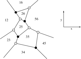
   Figure 14. A soliton graph $G_{{\bm{t}}}(\mathcal{M})$ coming from $\operatorname{Gr}(2,6)$.

   In [KW14, Theorem 8.5 and Theorem 8.9], the authors classified the contour plots $\mathcal{C}_{{\bm{t}}}(\mathcal{M})$ obtained when ${\bm{t}}=(t_{3},0,\dots,0)$ and $t_{3}\to\pm\infty$. We can now give a generalization of their results (cf. Corollary 8.11) in the case that $\mathcal{M}={[n]\choose k}$ and the $\kappa_{i}$’s are positive. Let us write ${\bm{t}}\geq 0$ if $t_{i}\geq 0$ for $i=3,\dots,n$.

   Proposition 8.10.

   Assume that $\mathcal{M}={[n]\choose k}$, the numbers $\kappa_{1}<\dots<\kappa_{n}$ are positive, and that the vector ${\bm{t}}\geq 0$ is nonzero. Then $\mathcal{C}_{{\bm{t}}}(\mathcal{M})$ can be identified with the plabic graph associated to the Le-diagram, and its regions are labeled by the elements of $\mathcal{F}(\mathcal{A},k,{\bm{h}}^{(w)})$ for $w=w_{0}$ as in Example 7.13. Similarly, the regions of $\mathcal{C}_{-{\bm{t}}}(\mathcal{M})$ are labeled by the elements of $\mathcal{F}(\mathcal{A},k,{\bm{h}}^{(w)})$ for $w=\operatorname{id}$.

   Proof.

   Recall that ${\bm{v}}_{i}=(\kappa_{i},\kappa_{i}^{2},1)$ and $h_{i}=\kappa_{i}^{3}t_{3}+\dots+\kappa_{i}^{n}t_{n}$. Our goal is to show that $h_{n}\gg h_{n-1}\gg\dots\gg h_{1}$ in the sense of (7.3). In other words, we need to show that $\mu_{\bm{h}}(a,b,c,d)<0$ for all $1\leq a<b<c<d\leq n$. For $3\leq j\leq n$, let ${{\bm{h}}^{(j)}}\in\mathbb{R}^{n}$ be given by ${h_{i}^{(j)}}:=\kappa_{i}^{j}t_{j}$, thus ${\bm{h}}=\sum_{j=3}^{n}{{\bm{h}}^{(j)}}$. It suffices to show $\mu_{{{\bm{h}}^{(j)}}}(a,b,c,d)<0$. It follows from (7.2) and (5.4) that

   $$\mu_{{{\bm{h}}^{(j)}}}(a,b,c,d)=-\det\left(\begin{smallmatrix}1&1&1&1\\ \kappa_{a}&\kappa_{b}&\kappa_{c}&\kappa_{d}\\ \kappa_{a}^{2}&\kappa_{b}^{2}&\kappa_{c}^{2}&\kappa_{d}^{2}\\ t_{j}\kappa_{a}^{j}&t_{j}\kappa_{b}^{j}&t_{j}\kappa_{c}^{j}&t_{j}\kappa_{d}^{j}\\ \end{smallmatrix}\right)=-t_{j}\cdot K_{\{a,b,c,d\}}\cdot s_{(j-3)}(\kappa_{a},\kappa_{b},\kappa_{c},\kappa_{d}),$$

   where $K_{\{a,b,c,d\}}$ was defined in (8.3) and $s_{\lambda}$ is the Schur polynomial associated with a partition $\lambda=(\lambda_{1},\dots,\lambda_{m})$, see [Sta99, §7.15]. Thus $s_{(j-3)}=h_{j-3}$ is the complete homogeneous symmetric polynomial [Sta99, §7.5]. Since $\kappa_{1}<\dots<\kappa_{n}$, we find $K_{\{a,b,c,d\}}>0$. Since we have also assumed that $\kappa_{1},\dots,\kappa_{n}>0$, we find $s_{(j-3)}(\kappa_{a},\kappa_{b},\kappa_{c},\kappa_{d})>0$. We have shown $\mu_{{{\bm{h}}^{(j)}}}(a,b,c,d)<0$ for all $j$ such that $t_{j}>0$, which implies $\mu_{\bm{h}}(a,b,c,d)<0$. For the case of $\mathcal{C}_{-{\bm{t}}}(\mathcal{M})$, the same argument shows $\mu_{\bm{h}}(a,b,c,d)>0$. ∎

   In Proposition 8.10, we required the $\kappa$-parameters to be positive. For the case ${\bm{t}}=(t_{3},0,\dots,0)$ studied in [KW14], this assumption can be lifted.

   Corollary 8.11.

   Proposition 8.10 still holds when the numbers $\kappa_{1}<\dots<\kappa_{n}$ are not necessarily positive, provided that ${\bm{t}}=(t_{3},0,\dots,0)$ with $t_{3}>0$.

   Proof.

   Indeed, in this case the polynomial $s_{(j-3)}=s_{(0)}$ from the proof of Proposition 8.10 is equal to $1$, thus we have $\mu_{\bm{h}}(a,b,c,d)<0$ regardless of the sign of the $\kappa$-parameters. ∎

   Since the generic soliton graphs $G_{{\bm{t}}}(\mathcal{M})$ for $\mathcal{M}={[n]\choose k}$ are trivalent $(k,n)$-plabic graphs, it is natural to ask which $(k,n)$-plabic graphs are realizable as soliton graphs. Similarly to Section 2.3, let us say that a bipartite $(k,n)$-plabic graph is realizable if it can be obtained from some $G_{{\bm{t}}}(\mathcal{M})$ by contracting unicolored edges. Thus every realizable $(k,n)$-plabic graph is also $\mathcal{A}$-regular for some $\mathcal{A}$. (It is not clear to us whether the converse is true.) In [KW11, KW14], the authors showed that all bipartite $(2,n)$-plabic graphs are realizable. In [KK18], building on work of [Hua15], Karpman and Kodama showed that for $k=3$ and $n=6,7,8$, every bipartite $(k,n)$-plabic graph is realizable for some choice of $\kappa$- and ${\bm{t}}$-parameters (see however Example 7.9 and [KK18, Theorem 4.2]).

References

- [ACEP19] Federico Ardila, Federico Castillo, Christopher Eur, and Alexander Postnikov. Coxeter submodular functions and deformations of Coxeter permutahedra. arXiv:1904.11029v1, 2019.
- [AHBC+16] Nima Arkani-Hamed, Jacob Bourjaily, Freddy Cachazo, Alexander Goncharov, Alexander Postnikov, and Jaroslav Trnka. Grassmannian Geometry of Scattering Amplitudes. Cambridge University Press, 2016. Preliminary version titled “Scattering Amplitudes and the Positive Grassmannian” at arXiv:1212.5605.
- [BLVS+99] Anders Björner, Michel Las Vergnas, Bernd Sturmfels, Neil White, and Günter M. Ziegler. Oriented matroids, volume 46 of Encyclopedia of Mathematics and its Applications. Cambridge University Press, Cambridge, second edition, 1999.
- [BS92] Louis J. Billera and Bernd Sturmfels. Fiber polytopes. Ann. of Math. (2), 135(3):527–549, 1992.
- [BS94] Louis J. Billera and Bernd Sturmfels. Iterated fiber polytopes. Mathematika, 41(2):348–363, 1994.
- [BW18] Alexey Balitskiy and Julian Wellman. Flips in reduced plabic graphs. MIT SPUR Final Project, https://math.mit.edu/research/undergraduate/spur/documents/2018Wellman.pdf, 2018.
- [BW19] Alexey Balitskiy and Julian Wellman. Flip cycles in plabic graphs. arXiv:1902.01530v2, 2019.
- [CK08] Sarbarish Chakravarty and Yuji Kodama. Classification of the line-soliton solutions of KPII. J. Phys. A, 41(27):275209, 33, 2008.
- [Eln97] Serge Elnitsky. Rhombic tilings of polygons and classes of reduced words in Coxeter groups. J. Combin. Theory Ser. A, 77(2):193–221, 1997.
- [Far] Miriam Farber. Personal communication.
- [FG18] Miriam Farber and Pavel Galashin. Weak separation, pure domains and cluster distance. Selecta Math. (N.S.), 24(3):2093–2127, 2018.
- [FZ99] Sergey Fomin and Andrei Zelevinsky. Double Bruhat cells and total positivity. J. Amer. Math. Soc., 12(2):335–380, 1999.
- [Gal18] Pavel Galashin. Plabic graphs and zonotopal tilings. Proc. Lond. Math. Soc. (3), 117(4):661–681, 2018.
- [GKZ94] I. M. Gel’fand, M. M. Kapranov, and A. V. Zelevinsky. Discriminants, resultants, and multidimensional determinants. Mathematics: Theory & Applications. Birkhäuser Boston, Inc., Boston, MA, 1994.
- [GP17] Pavel Galashin and Alexander Postnikov. Purity and separation for oriented matroids. arXiv:1708.01329v1, 2017.
- [GP18] Pavel Galashin and Pavlo Pylyavskyy. Ising model and the positive orthogonal Grassmannian. arXiv:1807.03282v3, 2018.
- [GS87] I. M. Gel’fand and V. V. Serganova. Combinatorial geometries and the strata of a torus on homogeneous compact manifolds. Uspekhi Mat. Nauk, 42(2(254)):107–134, 287, 1987.
- [Hir04] Ryogo Hirota. The direct method in soliton theory, volume 155 of Cambridge Tracts in Mathematics. Cambridge University Press, Cambridge, 2004. Translated from the 1992 Japanese original and edited by Atsushi Nagai, Jon Nimmo and Claire Gilson, With a foreword by Jarmo Hietarinta and Nimmo.
- [Hua15] J. Huang. Classification of soliton graphs on totally positive Grassmannian. 2015. Thesis (Ph.D.)–Ohio State University.
- [KK18] R. Karpman and Y. Kodama. Triangulations and soliton graphs for totally positive Grassmannian, 2018. preprint, arXiv:1808.01587.
- [Kod10] Yuji Kodama. KP solitons in shallow water. J. Phys. A, 43(43):434004, 54, 2010.
- [KP70] B. Kadomtsev and V. Petviashvili. On the stability of solitary waves in weakly dispersive media. Sov. Phys. - Dokl., (15):539–541, 1970.
- [KW11] Y. Kodama and L. K. Williams. KP solitons, total positivity, and cluster algebras. Proc. Natl. Acad. Sci. USA, 108(22):8984–8989, 2011.
- [KW14] Yuji Kodama and Lauren Williams. KP solitons and total positivity for the Grassmannian. Invent. Math., 198(3):637–699, 2014.
- [Lam18] Thomas Lam. Electroid varieties and a compactification of the space of electrical networks. Adv. Math., 338:549–600, 2018.
- [LP] Nan Li and Alexander Postnikov. In preparation.
- [MS89] Yu. I. Manin and V. V. Schechtman. Arrangements of hyperplanes, higher braid groups and higher Bruhat orders. In Algebraic number theory, volume 17 of Adv. Stud. Pure Math., pages 289–308. Academic Press, Boston, MA, 1989.
- [OEI] OEIS Foundation Inc. (2019), The On-Line Encyclopedia of Integer Sequences, http://oeis.org.
- [OPS15] Suho Oh, Alexander Postnikov, and David E. Speyer. Weak separation and plabic graphs. Proc. Lond. Math. Soc. (3), 110(3):721–754, 2015.
- [OS19] Jorge Alberto Olarte and Francisco Santos. Hypersimplicial subdivisions. arXiv:1906.05764v1, 2019.
- [Pos06] Alexander Postnikov. Total positivity, Grassmannians, and networks. Preprint, http:// math.mit.edu/~apost/papers/tpgrass.pdf, 2006.
- [Pos09] Alexander Postnikov. Permutohedra, associahedra, and beyond. Int. Math. Res. Not. IMRN, (6):1026–1106, 2009.
- [Pos18] Alexander Postnikov. Positive Grassmannian and polyhedral subdivisions. arXiv:1806.05307v1, 2018.
- [Pou14] Lionel Pournin. The diameter of associahedra. Adv. Math., 259:13–42, 2014.
- [PRW08] Alex Postnikov, Victor Reiner, and Lauren Williams. Faces of generalized permutohedra. Doc. Math., 13:207–273, 2008.
- [RW17] Konstanze Rietsch and Lauren Williams. Newton-Okounkov bodies, cluster duality, and mirror symmetry for Grassmannians. arXiv:1712.00447v2, 2017.
- [Sco05] Josh Scott. Quasi-commuting families of quantum minors. J. Algebra, 290(1):204–220, 2005.
- [Sco06] Joshua S. Scott. Grassmannians and cluster algebras. Proc. London Math. Soc. (3), 92(2):345–380, 2006.
- [She74] G. C. Shephard. Combinatorial properties of associated zonotopes. Canadian J. Math., 26:302–321, 1974.
- [Sta63] James Dillon Stasheff. Homotopy associativity of -spaces. I, II. Trans. Amer. Math. Soc. 108 (1963), 275-292; ibid., 108:293–312, 1963.
- [Sta77] Richard Stanley. Eulerian partitions of a unit hypercube. In Higher Combinatorics, page 49. Reidel, Dordrecht, 1977.
- [Sta99] Richard P. Stanley. Enumerative combinatorics. Vol. 2, volume 62 of Cambridge Studies in Advanced Mathematics. Cambridge University Press, Cambridge, 1999. With a foreword by Gian-Carlo Rota and appendix 1 by Sergey Fomin.
- [STT88] Daniel D. Sleator, Robert E. Tarjan, and William P. Thurston. Rotation distance, triangulations, and hyperbolic geometry. J. Amer. Math. Soc., 1(3):647–681, 1988.
- [Tam51] Dov Tamari. Monoïdes préordonnés et chaînes de Malcev. Thèse, Université de Paris, 1951.
- [VK91] V. A. Voevodsky and M. M. Kapranov. The free -category generated by a cube, oriented matroids and higher Bruhat orders. Funktsional. Anal. i Prilozhen., 25(1):62–65, 1991.
- [Zie93] Günter M. Ziegler. Higher Bruhat orders and cyclic hyperplane arrangements. Topology, 32(2):259–279, 1993.
- [Zie95] Günter M. Ziegler. Lectures on polytopes, volume 152 of Graduate Texts in Mathematics. Springer-Verlag, New York, 1995.
-
(iv)