Role of vector channel in different classes of (non) magnetized neutron stars

Abstract

We study how the magnetic field and non-standard vector channels affect hadronic, quark and hybrid stars. In the hadronic phase, we use the QHD model, with its standard $\sigma\omega\rho$ mesons, and compare the results with the ones obtained with the inclusion of the strangeness hidden $\phi$ meson. In the quark phase, we use the standard SU(3) NJL and compare the results with the version that takes into account the vector channel $G_{v}(\bar{\psi}\gamma^{\mu}\psi)$. Magnetic fields are taken into account via chaotic magnetic field approximation.

I Introduction

Super-powered pulsars with a magnetic field reaching as high as $10^{15}$ G in the surface and yet, values beyond $10^{18}$ G in their cores (due to the scalar Viral theorem Shapiro ) are believed to exist in nature. The idea of such magnetic field several times stronger than the ones usually found in pulsars were proposed by Duncan in Duncan1 ; Duncan2 to explain two distinct objects: soft gamma-ray repeaters (SGRs) and anomalous X-ray pulsars (AXPs). Up to date, both objects are believed to be different manifestation of a single type of compact star: the magnetar Sandro . A catalogue with updated information on magnetars can be found in catalogue . Presently, it contains data on 15 SGRs and 14 AXPs.

To describe a magnetar we revisit the theory of neutron stars, dense objects that are maintained by the equilibrium of gravity and the degeneracy pressure of the fermions. To explain the high masses observed, besides the degeneracy pressure, there must be another repulsive channel. Today it is well known that the baryon interaction is repulsive at extremely short distances. In the present work, we have divided the magnetars in three different possible types.

The first one is a hadronic neutron star - or simply neutron star for short - described within the Quantum hadrodynamics (QHD) formalism Serot . In this model the baryon interaction is mediated by scalar and vector mesons exchange. Within the QHD, we construct an equation of state (EoS), a relation between pressure and energy density. With the EoS in hand, we use the Tolman-Oppenheimer-Volkoff (TOV) equations TOV to obtain the macroscopic properties of the neutron stars. We also allow the hyperon onset in the nuclear bulk due to the high densities reached in the neutron star core. The possibility of the hyperon formation is, to some extent, an open puzzle Glen ; Lopes2013 ; Fortin2017 ; Oertel2016 ; Debi2016 . Recently, it was shown that the hyperon threshold can be suppressed by either very fast rotation Negreiros_2013 or by strong magnetic fields in a formalism that allows the coupling of Maxwell–Einstein equations in a self consistent way Lorene ; Dex4 . These conditions, however, are not expected in most of the observed pulsars and the cases studied so far show that the results are model dependent. We also dedicate an entire section to describe the role of the non-standard $\phi$ meson, a repulsive strangeness hidden channel, which is relevant to describe massive hyperonic stars.

On the other hand, once the internal composition of the neutron stars is not fully established, our second research considers the possibility that the compact stars are actually quark stars, composed of deconfined quarks. This proposal is based on the Bodmer-Witten conjecture Witten ; Bodmer , which states that strange matter is actually the ground state of all matter at high densities. If this is true, the entire star is converted into quark matter in a finite amount of time.

Moreover, even if strange matter is not the ground state, quarks can still be present in the core surrounded by hadronic matter. This is the third star type, called hybrid star. A nice argument to corroborate this idea is based on the large $N_{c}$ expansion as shown in ref.Mc . As the quark chemical potential exceeds the constituent quark mass, the increase of the pressure produces a phase where chiral symmetry is restored. With this hypothesis, for sufficiently high densities this matter becomes strange quark matter.

We study quark and hybrid star formalism within the three flavors SU$(3)$ Nambu Jona Lasinio (NJL) model Nambu ; Deb2009 ; DebJCAP2019 ; Lopes2016 , which is known to satisfy expected QCD chiral symmetry aspects. As in the case of hadronic stars, we dedicate an entire section to describe the role of the non-standard $G_{v}$ coupling, a repulsive vector channel which stiffens the EoS.

The role of the magnetic field on the neutron star properties is nowadays a very active field  Dex2018 ; Lalit ; Lee ; GusakovPRD ; Dex5 ; Dex6 ; Ro2017 ; Mauro . In the present work, the influence of the magnetic field is studied in the context of the chaotic magnetic field approximation Zel ; Lopes2015 ; china ; Lopes2016 , which allows us to construct a thermodynamic consistent pressure. There is no doubt that the ideal situation is to use the LORENE code Lorene ; Dex2018 ; Dex5 ; Dex6 ; Ro2017 , which performs a numerical computation of the neutron star by taking into account Einstein-Maxwell equations and equilibrium self consistently. Unfortunately, this calculation is not always feasible for all purposes, besides the very high computational price inherent to it. As already shown isop , the pressure needs to be a scalar and the chaotic magnetic field fulfills this requirement and avoids anisotropies Lopes2015 ,  as it yields a locally effective isotropic pressure Mauro . Moreover, the chaotic magnetic field satisfies some constraints related to the distribution of the magnetic field in magnetar interiors, as discussed in ref. debi2018 . Additional discussion about the validity of the chaotic magnetic field approximation can be found at scope and at the end of the manuscript.

II Magnetars as neutron stars

The natural tool to describe strong interacting matter is the quantum chromodynamics (QCD), which describes the interaction of quarks and gluons. However, except at a very narrow region of low density and high temperature - which turned out to be the opposite of what one would expect in neutron stars interiors - the Lattice QCD (LQCD) produces no results. To overcome this issue, we use effective models. Here we present the quantum hadrodynamics (QHD). The QHD considers the baryons as the fundamental degrees of freedom and describes their interactions via mesons exchange Serot .

To produce reliable neutron star properties we need to be able to reproduce realistic physical quantities that are known from phenomenology. There are five well known properties of symmetric nuclear matter at the saturation point: the saturation density itself ($n_{0}$), the effective nucleon mass ($M^{*}/M$), the compressibility $(K)$, the symmetry energy ($S_{0}$) and the binding energy per baryon ($B/A$) Glen . Besides them, it is also worth noticing that the study of the slope of the symmetry energy ($L$) - which has non-negligible implications on the neutron star macroscopic properties - has had a great development in the last years, although the debate about its true value is still going on Rafa ; Lopes2014 ; Tsang ; Micaela2017 ; Lattimer2014 ; Pais2016 ; Dex2019 ; Prov2019 . To fulfill this constraint we use a slightly modified GM1 parametrization, which reduces the slope from 94 MeV to 88 MeV by reducing $(g_{N\rho}/m_{\rho})^{2}$ from its original value of 4.410 fm² to 3.880 fm². This modification also causes a small reduction in the symmetry energy from 32.5 MeV to 30.5 MeV.

The QHD Lagrangian in this work reads (Eq. (1)):

$$\mathcal{L}_{QHD}=\sum_{b}\bar{\psi}_{b}\bigg{[}\gamma^{\mu}(i\partial_{\mu}-e_{b}A_{\mu}-g_{b,\omega}\omega_{\mu}-g_{b,\rho}\frac{1}{2}\vec{\tau}\cdot\vec{\rho}_{\mu})-(m_{b}-g_{b,\sigma}\sigma)\bigg{]}\psi_{b}+\frac{1}{2}m_{v}^{2}\omega_{\mu}\omega^{\mu}$$

$$+\frac{1}{2}m_{\rho}^{2}\vec{\rho}_{\mu}\cdot\vec{\rho}^{\;\mu}+\frac{1}{2}(\partial_{\mu}\sigma\partial^{\mu}\sigma-m_{s}^{2}\sigma^{2})-U(\sigma)-\frac{1}{4}F^{\mu\nu}F_{\mu\nu}-\frac{1}{4}\Omega^{\mu\nu}\Omega_{\mu\nu}-\frac{1}{4}\bf{P}^{\mu\nu}\cdot\bf{P}_{\mu\nu},$$ (1)

in natural units. $\psi_{b}$ are the baryonic Dirac fields. Here, not only nucleons can be present, but we also consider the possibility of hyperon creation in neutron star core. Because of the Pauli principle, as the number density increases, so does the Fermi energy. Ultimately the Fermi energy of the nucleons exceeds the mass of heavier baryons, and the conversion of some nucleons into hyperons Glen become energetically favorable. The $\sigma$, $\omega_{\mu}$ and $\vec{\rho}_{\mu}$ are the mesonic fields. The $g^{\prime}s$ are the Yukawa coupling constants that simulate the strong interaction, $m_{b}$ is the mass of the baryon $b$, $m_{s}$, $m_{v}$, and $m_{\rho}$ are the masses of the $\sigma$, $\omega$, and $\rho$ mesons respectively, $e_{b}$ is the electric charge of the baryon $b$, $A_{\mu}$ is the electromagnetic four-potential and $\vec{\tau}$ are the Pauli matrices. The antisymmetric mesonic field strength tensors are given by their usual expressions as presented in Glen , i.e., $F^{\mu\nu}=(\partial^{\mu}A^{\nu}-\partial^{\nu}A^{\mu})$, $\Omega^{\mu\nu}=(\partial^{\mu}\omega^{\nu}-\partial^{\nu}\omega^{\mu})$ and $\bf{P}_{\mu\nu}=(\partial_{\mu}\overrightarrow{\rho}_{\nu}-\partial_{\nu}\overrightarrow{\rho}_{\mu})-g_{\rho}(\overrightarrow{\rho}_{\mu}\times\overrightarrow{\rho}_{\nu})$. The $U(\sigma)$ is the self-interaction term introduced in ref. Boguta to reproduce some of the saturation properties of the nuclear matter and is given by:

$$U(\sigma)=\frac{1}{3!}\kappa\sigma^{3}+\frac{1}{4!}\lambda\sigma^{4}.$$ (2)

As magnetars are stable macroscopic objects, we need to describe a neutral, chemically stable matter and hence, leptons are added as free Fermi gases described by

$$\mathcal{L}_{lep}=\sum_{l}\bar{\psi}_{l}[i\gamma^{\mu}(\partial_{\mu}-e_{l}A_{\mu})-m_{l}]\psi_{l},$$ (3)

where the sum runs over the two lightest leptons ($e$ and $\mu$).

Let us now give the parameters of the GM1 model as well as the prediction of the physical quantities and their inferred values from phenomenology Glen ; Glen2 ; Dutra2014 ; Micaela2017 . In Tab. (1) we resume these values.

	Parameters		Phenomenology	GM1	Masses ($MeV$)
$(g_{N\sigma}/m_{s})^{2}$	11.785 $fm^{2}$	$n_{0}$ ($fm^{-3}$)	0.148 - 0.170	0.153	$M_{\Lambda}$ = 1116
$(g_{N\omega}/m_{v})^{2}$	7.148 $fm^{2}$	$M^{*}/M$	0.7 - 0.8	0.7	$M_{\Sigma}$ = 1193
$(g_{N\rho}/m_{\rho})^{2}$	3.880 $fm^{2}$	$K$ ($MeV$)	200 - 315	300	$M_{\Xi}$ = 1318
$\kappa/M_{N}$	0.005894	$S_{0}$ ($MeV$)	30 - 34	30.5	$m_{e}$ = 0.511
$\lambda$	-0.006426	$B/A$ ($MeV$)	15.7 - 16.5	16.3	$m_{\mu}$ = 105.6
$M_{N}$	939 $MeV$	$L$ ($MeV$)	36 - 113	88	-

Table 1: GM1 model parameters and physical quantities infered from experiments Glen2 ; Dutra2014 ; Micaela2017 .

As we allow the hyperon onset we also have to fix the hyperon-mesons coupling constants. Unlike the nuclear matter, we have very little experimental information about hyperonic matter. The main term is the hyperon potential depth fixed at the saturation density. However, just the $\Lambda$ hyperon has the potential depth well fixed at -28 $MeV$ Glen2 . The knowledge of the other potential depths are known with a lower degree of precision. Unfortunately the knowledge of the hyperon potential depth is not enough to fix all constants, once different sets of coupling constants reproduce the same potential values. Even worst is the fact that these different sets of the coupling constants, yet predicting the same potential depth, cause large variations on the neutron star properties Glen . So, in order to reduce the large number of free parameters we fix the well known $\Lambda$ potential depth $U_{\Lambda}$ = -28 $MeV$, and use symmetry group theory to fix all the other hyperon-meson coupling constants. To be more specific, we use the hybrid SU(6) group Pais to fix all the vector mesons and a nearly SU(6) group to fix the scalar ones as presented in Lopes2013 . All the hyperon-mesons coupling constants are presented bellow in Eq. (4).

$$\frac{g_{\Lambda\omega}}{g_{N\omega}}=\frac{g_{\Sigma\omega}}{g_{N\omega}}=0.667,\quad\frac{g_{\Xi\omega}}{g_{N\omega}}=0.333,$$ (4)

$$\frac{g_{\Sigma\rho}}{g_{N\rho}}=2.0\quad\frac{g_{\Xi\rho}}{g_{N\rho}}=1.0,\quad\frac{g_{\Lambda\rho}}{g_{N\rho}}=0.0,$$

$$\frac{g_{\Lambda\sigma}}{g_{N\sigma}}=0.610,\quad\frac{g_{\Sigma\sigma}}{g_{N\sigma}}=0.396,\quad\frac{g_{\Xi\sigma}}{g_{N\sigma}}=0.113.$$

To solve the equations of motion, we use the mean field approximation (MFA), where the meson fields are replaced by their expectation values, i.e: $\sigma$ $\to$ $\left<\sigma\right>$ = $\sigma_{0}$, $\omega^{\mu}$ $\to$ $\delta_{0\mu}\left<\omega^{\mu}\right>$ = $\omega_{0}$ and $\rho^{\mu}$ $\to$ $\delta_{0\mu}\left<\rho^{\mu}\right>$ = $\rho_{0}$. Applying the Euler-Lagrange formulation to Eq. (1) we obtain, for a baryon in the absence of electric field, the following equation of motion:

$$[\gamma_{0}(i\partial^{0}-g_{b,\omega}\omega_{0}-g_{b,\rho}\rho_{0})-\gamma_{j}(i\partial^{j}-e_{b}A^{j})-M^{*}_{b}]\Psi=0,$$ (5)

where we define $M^{*}_{b}~{}\doteq~{}m_{b}-g_{b,\sigma}\sigma_{0}$ as the effective baryon mass.

For an uncharged baryon, $e_{b}A^{j}$ is always zero. Using the quantization rules ($E=i\partial^{0}$, $i\partial^{j}=k$) we easily obtain the eigenvalue for the energy:

$$E_{b}=\sqrt{k^{2}+M^{*2}_{b}}+g_{b,\omega}\omega_{0}+g_{B,\rho}\frac{\tau_{3}}{2}\rho_{0}.$$ (6)

In the case of magnetars, as expected, the magnetic field plays a crucial role. So, to study its effect, we start with a static external magnetic field in the $z$ direction (these conditions will be relaxed latter). To accomplish that we fix: $A_{2}=A_{3}=0;A_{1}=-B_{0}y$. This choice results in a quantum harmonic oscillator like equation, whose eigenvalue solution is well known  Lopes2012 ; Pal ; Peng ; Rhabi :

$$E_{b}=\sqrt{k_{z}^{2}+M^{*2}_{b}+2\nu|e|B_{0}}+g_{b,\omega}\omega_{0}+g_{B,\rho}\frac{\tau_{3}}{2}\rho_{0},$$ (7)

where $\nu$ is a discrete parameter called Landau level (LL). For the leptons, since they are all charged and are not affected by the strong force, we have:

$$E_{l}=\sqrt{k_{z}^{2}+m^{2}_{l}+2\nu|e|B_{0}}.$$ (8)

To construct the equation of state (EoS) for this many body system of leptons and strongly interacting baryons we use the Fermi-Dirac statistics. As the thermal energy of a stable neutron star is much lower than the Fermi energy of its particles, $T=0$ is a good approximation. For the uncharged baryons the distribution is isotropic and the solution for the energy density is straightforward Greiner2 :

$$\epsilon=\frac{1}{\pi^{2}}\int_{0}^{k_{f}}\sqrt{k^{2}+M^{*}_{b}}k^{2}dk.$$ (9)

For the charged fermions (baryons and leptons), not only the energy spectrum is quantized but also the distribution in the plane perpendicular to the magnetic field. In this case the energy density reads Lopes2012 ; Peng :

$$\epsilon=\frac{|e|B_{0}}{2\pi^{2}}\sum_{\nu}\eta(\nu)\int_{0}^{k_{f}}\sqrt{k_{z}^{2}+M^{*}_{b}+2\nu|e|B_{0}}dk_{z},$$ (10)

where $k_{f}$ is the Fermi momenta of the particle and $\eta(\nu)$ is the degeneracy of the LL $\nu$. The first Landau Level is non-degenerate and the others are two-fold degenerate. The sum over the LL ends at the closest integer at which the square of the Fermi momenta of the particle is still positive.

In MFA the contribution of the mesonic fields to the energy density is given by Glen ; Lopes2012 ; Lopes2013

$$\epsilon_{m}=\frac{1}{2}\bigg{(}m_{s}^{2}\sigma_{0}^{2}+m_{v}^{2}\omega_{0}^{2}+m_{\rho}^{2}\rho_{0}^{2}\bigg{)}+U(\sigma),$$ (11)

The total energy density is the sum of the energy density of all fields (baryons, leptons and mesons). Finally the expected values of the mesonic fields are calculated either from the Euler-Lagrange equations or by imposing that the total energy density be stationary at fixed baryon density Glen :

$$\bigg{(}\frac{\partial\epsilon}{\partial\sigma_{0}}\bigg{)}=\bigg{(}\frac{\partial\epsilon}{\partial\omega_{0}}\bigg{)}=\bigg{(}\frac{\partial\epsilon}{\partial\rho_{0}}\bigg{)}=0.$$ (12)

To calculate every particle population at a fixed density we impose electric charge neutrality and chemical equilibrium:

$$\mu_{bi}=\mu_{n}-e_{bi}\mu_{e},\mu_{\mu}=\mu_{e};\quad\sum_{f}e_{f}n_{f}=0,$$ (13)

where $\mu_{bi}$ and $e_{bi}$ are the chemical potential and electric charge of the i-th baryon respectively. At zero temperature, the chemical potentials coincide with the energy eigenvalues given in Eqs. (6) and (7); $\mu_{e}$ and $\mu_{\mu}$ are the electron and muon chemical potential respectively; $n$ is the number density and the sum in $f$ runs over the two fermions.

Now, to construct the EoS we calculate the pressure via thermodynamics:

$$p=\sum_{f}\mu_{f}n_{f}-\epsilon,$$ (14)

where the sum runs over all fermions.

II.1 Contribution of the magnetic field itself

Now let’s take a closer look at the magnetic field itself. As we known from Einstein’s general relativity, every form of energy should be taken into account via the energy-momentum tensor. As the magnetic field itself has energy it will ultimately contribute in the TOV equations TOV . Although its contribution to the energy is simple, the contribution to the pressure is not trivial. The reason is that for a constant magnetic field in the $z$ direction, the stress tensor is not diagonal, but reads $B=diag(B^{2}/2,B^{2}/2,-B^{2}/2)$ Gravitation .

The straightforward way to solve this problem is a fully relativistic numerical integration of Einstein’s field equations. However it demands a very high computational price. Once we are in the realm of effective fields, we can look for options. The standard approach in the literature Lopes2012 ; Ryu ; Panda ; Mallick ; Dex1 ; Casali ; Dex2 ; Dex3 is to consider only the perpendicular component of the pressure. In this case, the contribution of the pressure is equal to the contribution of the energy, $p=\epsilon=B^{2}/2)$. However, this approach cannot be justified by first principles, overestimates the influence of the magnetic field and is in disagreement with more precise calculations Lorene ; debi2018 . Another common approach is to split the pressure into two parts, the so called perpendicular and parallel pressures and then solve an axisymmetric version of the TOV equations Mallick2 ; Zubairi ; Paret . However this approach has a big issue once the thermodynamical concept of pressure cannot depend on the direction because it is a scalar. Also, it was already discussed in the literature that the pressure is ultimately isotropic even in the presence of a magnetic field isop . Besides the problem of the thermodynamical consistency in the presence of a magnetic field, there is also a problem regarding the stability of the magnetic field itself. As discussed in the literature, an uniform magnetic field in the $z$ direction is unstable insta1 ; insta2 . A way to avoid both problems lies in the concept of chaotic magnetic field, as originally introduced by Zeldovich Zel in the 60’s: “It is possible to describe the effect of the magnetic field by using the pressure concept only when we are dealing with a small-scale chaotic field (pag. 158)”. So we relax the condition of an uniform magnetic field in the $z$ direction and assume the chaotic magnetic field, whose stress tensor reads: $diag(B^{2}/6,B^{2}/6,B^{2}/6)$, thus avoiding the anisotropy problem and yielding $p=\epsilon/3$, a radiation pressure formalism. Within this approach the contribution of the magnetic field to the EoS reads Lopes2015 ; china :

$$\epsilon=\epsilon_{M}+\frac{B_{0}^{2}}{2}\quad;\quad p=p_{M}+\frac{B_{0}^{2}}{6},$$ (15)

where $M$ stands for the matter.

We now go back to the issue of an uniform magnetic field. The more powerful magnetars are expected to have a magnetic field around $10^{15}G$ in their surface Duncan1 ; Duncan2 . Although fields of these magnitudes do not affect the main properties of neutron stars, fields larger than $10^{18}G$ are expected in the magnetar core due to the scalar Virial theorem Shapiro . To simulate the magnetic field growing towards the core we use an energy density dependent approach, as introduced in Lopes2015 :

$$B(\epsilon)=B_{0}\bigg{(}\frac{\epsilon_{M}}{\epsilon_{c}}\bigg{)}^{\gamma}+B_{surf},$$ (16)

where $\epsilon_{M}$ is the matter energy density and $\epsilon_{c}$ is the energy density at the core for zero magnetic field configuration, $B_{surf}$ is the magnetic field at the surface of the magnetar, for which we use $10^{15}G$, $B_{0}$ is the maximum magnetic field expected in the core, which we consider to be of the order of 3 $\times$ $10^{18}G$ to account for the scalar Virial theorem, and $\gamma$ is the only free parameter of our model. To study its influence on the neutron star properties, we use $\gamma$ = 4 and $\gamma$ = 6. Now $B(\epsilon)$ replaces $B_{0}$ in Eq. (15), only in the therm of self-energy - $B^{2}/2$ and $B^{2}/6$ - , but not in the matter term. We make this choice for two reasons: assure that the energy eigenvalue is correct, and the fact that using a variable magnetic field also in the matter does not significantly affect the results as showed in ref. Casali . Concerning this approach, a word of caution is important: a density dependent magnetic field violates Maxwell equations as discussed in alloy and a rearrangement term, never calculated, would be necessary. Moreover, as the chaotic magnetic field is spherically symmetric, neutron star deformations are beyond the scope of this work. To study deformations and deviations from the spherical symmetry, one needs to use poloidal magnetic fields as presented in ref. Dex5 ; Ro2017 , or even more complex geometries as a combination between toroidal and poloidal fields.

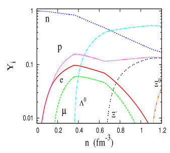
Figure 1: (Color online) Particle population for zero magnetic field (right) and for $B_{0}$ = 3 $\times 10^{18}G$ (left). The Landau quantization induces several kinks and descontinuities at small densities.

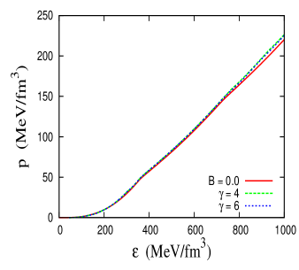
Figure 2: (Color online) (right) EoS and (left) mass-radius relation for a neutron star with zero magnetic field and two variations of density dependent magnetic fields. Within the chaotic magnetic field approximation the increase of the maximum mass is very small and the results are independent of the free parameters.

II.2 Results

We plot in Fig. (1) the particle population for zero magnetic field and $B_{0}=3\times 10^{18}G$. The hyperon population is strong dependent on the hyperon-meson coupling constants. With our choice that the couplings are constrained to the SU(6) symmetry group, we see that the $\Lambda^{0}$ is the first hyperon to appear around $n=0.35fm^{-3}$. Also, with this approach, the $\Sigma$ triplet is suppressed, the $\Xi^{-}$ appears around 0.66 $fm^{-3}$ while the onset of the $\Xi^{0}$ occurs at densities beyond those found in the neutron star core. When the magnetic field is present, two main differences arise in comparison with the results in non magnetized matter: the first one is that the charged particle population is favored at low densities since they are coupled to the magnetic field. The second is the presence of many kinks, especially at low densities due the dependence with the discrete LL. At low densities there are few LL available. As the density increases, the number of LL grows and approaches the continuum and the particle population is similar to those found in the absence of the magnetic field.

For the macroscopic properties of the neutron stars, we plot in Fig. (2) the EoS and mass-radius relation for zero magnetic field and a magnetic field of $3\times 10^{18}G$ within two different variations, with $\gamma$ = 4 and $\gamma$ = 6. In the absence of magnetic field, the maximum neutron star mass is 1.95 $M_{\odot}$ which is slightly below the limit of the PSR J0348+0432 in ref. Antoniadis . When the magnetic field is taken into account, the maximum mass increases to 1.98 $M_{\odot}$ which agrees with the measurement of PSR J0348+0432. Also, this small increase of the mass is in agreement with more complex models in different approaches as can be seen int Lorene ; Mallick2 ; Dex4 ; Ro2017 . Moreover, comparing the results for $\gamma$ = 4 and $\gamma$ = 6 we see that with the chaotic magnetic field, the variation of the magnetic field has very little influence on the macroscopic properties of the magnetars, a very reasonable result, once the $\gamma$ is a non-observable parameter. At the end of 2019 an even more massive pulsar was discovered, the MSP J0740+6620, which has a mass of $2.14^{+0.10}_{-0.09}$ at 68$\%$ credibility interval and $2.14^{+0.20}_{-0.18}$ at 95$\%$ credibility interval Cromartie . Although there is a small chance that its mass lies below 2 $M_{\odot}$, if it turns out to be above 2.1 $M_{\odot}$, a new formalism may be necessary to explain such massive pulsar Clesio .

Recent estimates of neutron star radii Hebeler ; Lattimer2013 point out that the canonical star (1.4 $M_{\odot}$) has a radius not much larger than 13 km. Although these results refer to non-magnetized neutron stars, we see that in our case, stars below 1.5 $M_{\odot}$ bear radii that are smaller than non-magnetized ones. These stars have a relatively low magnetic field; for instance, in our model a neutron star with a mass of 1.2 to 1.3 solar masses has a central magnetic field below $10^{17}~{}G$ Lopes2015 . However, as can be seen from Fig. (2), stars with masses above 1.6 solar masses have, in fact, larger radii than non-magnetized ones. For a 1.8 $M_{\odot}$ neutron star, its central magnetic field lies around 2-5 $\times 10^{17}~{}G$. The maximum magnetic field reached in the core of the maximum mass neutron star is also very close to the value of $B_{0}$, but never surpasses it. The main macroscopic properties of the maximum mass neutron stars, as well the radii of canonical 1.4 $M_{\odot}$ stars are plotted in Tab. (2).

$\gamma$	$M/M_{\odot}$	$R(km)$	$\epsilon_{c}$ ($MeV/fm^{3}$)	$B_{c}$ ($10^{18}G)$	$R_{1.4}(km)$
$B=0$	1.95	12.47	976	0.0	13.63
4	1.98	12.47	970	2.98	13.62
6	1.98	12.51	963	2.96	13.58

Table 2: Neutron stars main properties for zero magnetic field and two variations of density dependent magnetic fields, both with $B_{0}=3\times 10^{18}G$.

II.3 The importance of the vector channel

The GM1 parametrization, which is used in this work was fitted to describe the properties of nuclear matter at the saturation point. To describe the hyperon threshold in the neutron star core, a new set of hyperon-meson couplings was necessary. Due to our choice of the SU(6) symmetry group, only one free parameter was needed, which was fixed by the imposition that $U_{\Lambda}$ = -28 $MeV$. However, when hyperons are present not only new coupling constants arise, but also a new vector meson is possible, the strangeness-hidden $\phi$ meson, whose Lagrangian reads Lopes2013 ; Lopes2018 ; kapusta :

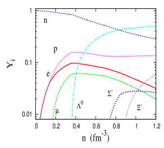
Figure 3: (Color online) Particle population for zero magnetic field and for $B_{0}$ = 3 $\times 10^{18}G.$ The $\phi$ meson causes the $\Sigma^{-}$ be present and pushes the $\Xi$’s to very high densities.

Figure 4: (Color online) EoS and Mass-radius relation for a neutron star with zero magnetic field and two variations of magnetars with the $\phi$ meson. All neutron stars results now agree with the PSR J0348+0432.

$$\mathcal{L}=g_{Y,\phi}\bar{\psi}_{Y}(\gamma^{\mu}\phi_{\mu})\psi_{Y}+\frac{1}{2}m_{\phi}^{2}\phi_{\mu}\phi^{\mu}-\frac{1}{4}\Phi^{\mu\nu}\Phi_{\mu\nu},$$ (17)

The $\phi$ meson is analogous to the $\omega$ meson and its expected value is also calculated via MFA Lopes2013 ; kapusta . As it is a vector meson, the $\phi$ field increases the repulsion between the hadrons and consequently increases the maximum neutron star mass. Nevertheless, adding a new meson implies on a new set of free parameters in the Lagrangian. However, using the SU(6) symmetry group, all hadron-$\phi$ couplings are already constrained and within this approach, no new free parameter is needed at all. From the symmetry group we have Lopes2013 :

$$\frac{g_{\Lambda\phi}}{g_{N\omega}}=\frac{g_{\Sigma\phi}}{g_{N\omega}}=-0.471,\quad\frac{g_{\Xi\phi}}{g_{N\omega}}=-0.943,$$ (18)

$$\quad\frac{g_{N\phi}}{g_{N\omega}}=0.0.$$

Now in Fig. (3) we plot the particle population for $\beta$-stable matter with the $\phi$ meson for zero magnetic field and for a magnetic field equal to 3 $\times$ $10^{18}$ G. For low densities, as the $\phi$ meson does not couple to the nucleon, there is no difference when compared to results without it. Once the $\Lambda$ appears, the $\phi$ field is no longer null and a new repulsion channel arises. As can be seen from Eq. (18), the repulsion of the $\Xi$ hyperons is stronger, which causes a suppression of these particles allowing the onset of the $\Sigma^{-}$ hyperon, which was absent when the $\phi$ meson was not taken into account. As in the last section, when a strong magnetic field is present, the particle densities are quantized due the LL and many kinks appear.

Now in Fig. (4) we plot the EoS and the mass-radius relation for neutron stars and magnetars with the $\phi$ meson. As the $\phi$ meson increases the hyperon chemical potentials, it reduces the strangeness fraction of the hyperons in neutron stars core. Moreover, the $\phi$ meson itself enters in the pressure calculation, causing the EoS to become stiffer. All these effects combined cause a significant stiffening and an increase in the maximum mass of non-magnetized neutron stars from 1.95 $M_{\odot}$ to 2.06$M_{\odot}$, which puts the neutron stars in agreement with the PSR J0348+0432 Antoniadis and even with MSP J0740+6620 Cromartie . It also causes an increase of the radii for stars above 1.9$M_{\odot}$, as they are near the maximum mass when the $\phi$ meson is absent, but not so near when it is included. As far as magnetars are concerned, when the magnetic field is present the maximum mass has a small rises from 2.06 $M_{\odot}$ to 2.07 $M_{\odot}$ and 2.08 $M_{\odot}$, depending of the value of $\gamma$ This shows that the chaotic magnetic field is a free-parameter way to introduce magnetic effects on the macroscopic properties of neutron stars.These small increase of the maximum mass are again in agreement of more complex calculations Dex3 ; Lorene . We resume the main properties of the neutron stars and magnetars with the $\phi$ meson in Tab. (3).

$\gamma$	$M/M_{\odot}$	$R(km)$	$\epsilon_{c}$ ($MeV/fm^{3}$)	$B_{c}$ ($10^{18}G)$	$R_{1.4}(km)$
B=0	2.06	11.96	1122	0.0	13.63
4	2.07	12.19	998	2.66	13.62
6	2.08	12.18	1060	2.83	13.58

Table 3: Neutron stars main properties for zero magnetic field and two variations of density dependent magnetic fields, both with $B_{0}=3\times 10^{18}G$ with the $\phi$ meson take into account.

To summarize this section, let’s say that we have studied the theory of magnetars as a hadronic neutron star, allowing the hyperon onset due the high densities reached in the core. Using the GM1 model for the nuclear matter and the symmetry group arguments to fix the hyperon-meson coupling constant we show that non-magnetized neutron stars can reach a maximum mass of 1.95$M_{\odot}$, which is subtly below the constraint of the PSR J0348+0432. This issue is solved when we consider the effects of magnetic field or the strangeness-hidden $\phi$ meson, which does not couple to the nucleon, and rises the maximum mass to 2.06$M_{\odot}$. The influence of the magnetic field is studied using the chaotic field approximation, and its effect is to always increase the maximum mass. Without the $\phi$ meson this increase is about $2\%$ and with it, the increase drops to only $1\%$. In all cases, the influence of the magnetic field seems independent of the non-observable parameter $\gamma$.

III Magnetars as quark stars

As stated out earlier, the true ground state of the hadronic matter might not be composed of protons and neutrons but rather, of strange quark matter, as predicted by Bodmer and Witten Bodmer ; Witten . If this is true, pulsars with central densities above a certain limit are quark stars, or strange stars. The main difference of quark stars to the conventional neutron stars, composed of baryons, is the fact that while the neutron star is bounded by gravity, the quark star is self-bounded, i.e, is the strong force that keeps matter cohesive against the degeneracy pressure of the quarks.

	Parameters		Phenomenology	SU(3) NLJ
$m_{u}=m_{d}$	5.5 $MeV$	$m_{\pi}$ ($MeV$)	128 -138	138
$m_{s}$	135.7 $MeV$	$m_{\eta}$ ($MeV$)	487	549
$\Lambda$	631.4 $MeV$	$m_{\sigma}$ ($MeV$)	668	700
$G_{s}\Lambda^{2}$	1.835	$f_{\pi}$ ($MeV$)	93	93
$K\Lambda^{5}$	9.29	$f_{\eta}$ ($MeV$)	94.3	84 - 102

Table 4: SU(3) NJL parameters and physical quantities infered from experiments Kun2 .

To describe a quark star we need to use a quark matter EoS. Again, the official tool to describe quarks via standard model is the QCD and once more we need an effective model. As the quark matter is expected to restore the chiral symmetry at high densities, we seek a model with this feature. To accomplish this task we use the SU(3) version of the NJL model Nambu ; DebPRC2009 ; DebPRC2014 . The SU(3) NJL Lagrangian includes a scalar, a pseudo-scalar and the t’Hooft six-fermion interaction - needed to model the axial symmetry breaking Kun1 ; Kun2 . Its Lagrangian density reads:

$$\mathcal{L}_{NJL}=\bar{\psi}_{f}[\gamma^{\mu}(i\partial_{\mu}-e_{f}A_{\mu})-m_{f}]\psi_{f}-\frac{1}{4}F_{\mu\nu}F^{\mu\nu}+$$

$$+G_{s}\sum_{a=0}^{8}[(\bar{\psi}\lambda_{a}\psi)^{2}+(\bar{\psi}\gamma_{5}\lambda_{a}\psi)^{2}]-K\{det[\bar{\psi}(1+\gamma_{5})\psi+det[\bar{\psi}(1-\gamma_{5})\psi]\}$$ (19)

where $\psi_{f}$ are the quark Dirac fields, with three flavors, $m_{f}$ = diag$(m_{u},m_{d},m_{s})$ are the current quark masses, $e_{f}$ represents the quark electric charge, $\lambda_{a}$ are the eight Gell-Mann flavor matrices and $G_{s}$ and $K$ are coupling constants. Unlike the QHD model for baryons, where the interaction is mediated by massive mesons, the NJL model has no mediator, and the interaction is a direct quark-quark point-like scheme (see ref. DebPRC2009 ; Kun2 to see the Feynman diagrams). This makes the NJL a non-renormalizable model, and a cutoff is needed to obtain physical results. The SU(3) NJL predicts five main physical parameters: the $\pi$, $\eta$ and $\sigma$ meson masses, as well pion and $\eta$ decay coupling constants, $f_{\pi}$ and $f_{\eta}$. The parameters, physical predictions and experimental values are given in Tab. (4).

Assuming mean field approximation (MFA) we can rewrite the quark-quark interaction in terms of the scalar condensates ($(\bar{\psi}\psi)2$ = $2\langle\bar{\psi}\psi\rangle-\langle\bar{\psi}\psi\rangle^{2})$ MB . To construct the EoS for quark matter, we need to construct the thermodynamical potential, once p = $-\Omega$. For each flavor, the pressure has three components, the in medium, the vacuum and the magnetic contribution ($p_{i}$ = $p^{med}_{i}+p^{vac}_{i}+p^{mag}_{i}$), besides the condensates ($\phi_{f}=\langle\bar{\psi}_{f}\psi_{f}\rangle$) that also contribute to the pressure. Following ref. Kun2 ; DebPRC2009 ; DebPRC2014 ; MB and assuming T = 0, we have:

$$\Omega=-\sum_{f}p_{f}+2G_{s}(\phi_{u}^{2}+\phi_{d}^{2}+\phi_{s}^{2})-4K\phi_{u}\phi_{d}\phi_{s},$$ (20)

where the contributions are:

$$p_{f}^{med}=\frac{N_{c}|e_{f}|B}{2\pi^{2}}\sum_{\nu}\eta(\nu)\int_{0}^{k_{f}}dk\frac{k^{2}}{E_{f}}$$

$$p_{f}^{vac}=\frac{N_{c}}{\pi^{2}}\int_{0}^{\Lambda}dk\epsilon_{v}k^{2}$$ (21)

$$p_{f}^{mag}=\frac{N_{c}(|e_{f}|B)^{2}}{2\pi^{2}}\bigg{[}\zeta^{\prime}(-1,x_{f})+$$

$$-\frac{(x_{f}^{2}-x_{f})}{2}\ln x_{f}+\frac{x_{f}^{2}}{4}\bigg{]},$$

where $N_{c}$ is the number of colors, $E_{f}$ = $\sqrt{M_{f}^{2}+k_{z}^{2}+2|e_{f}|B}$ is the energy eigenvalue for fermions under the influence of external magnetic fields and $M_{f}$ are the dynamical quark masses, which depend on the condensates:

$$M_{f}=m_{f}-4G_{s}\phi_{i}+2K\phi_{j}\phi_{k}.$$ (22)

The $\epsilon_{v}=\sqrt{k^{2}+M^{2}}$ can be seen as a vacuum energy eigenvalue, as it is very similar to the energy of free fermions; $\zeta^{\prime}$ is the derivative of the Riemann-Hurwitz zeta function and $x_{f}=M_{f}^{2}/(2|e_{f}|B)$. For more details on the formalism, please see ref. DebPRC2009 ; DebPRC2014 ; MB .

To finish, we need to calculate the value of the condensates. In the same way as the pressure, the condensates also have contributions from medium, vacuum, and the magnetic field ($\phi_{f}=\phi_{f}^{med}+\phi_{f}^{vac}+\phi_{f}^{mag})$. These values are:

$$\phi_{f}^{med}=\frac{N_{c}|e_{f}|BM_{f}}{2\pi^{2}}\sum_{\nu}\eta(\nu)\ln\bigg{(}\frac{E_{f}+k_{f}}{\sqrt{M_{f}^{2}+2|e_{f}|B}}\bigg{)}$$

$$\phi_{f}^{vac}=-\frac{N_{c}M_{f}}{2\pi^{2}}\bigg{[}\Lambda\epsilon_{v}-\frac{M_{f}^{2}}{2}\ln\bigg{(}\frac{\epsilon_{v}+\Lambda}{M^{2}}\bigg{)}\bigg{]}$$

(23)

$$\phi_{f}^{mag}=-\frac{M_{f}N_{c}(|e_{f}|B)^{2}}{2\pi^{2}}\bigg{[}\ln\Gamma(x_{f})-\frac{1}{2}\ln(2\pi)+$$

$$+x_{f}-\frac{(2x_{f}-1)}{2}\ln x_{f}\bigg{]}.$$

As the dynamical masses $M_{f}$ depend of the condensate values and vice-versa, these equations are solved in a self-consistently way. Equations (22) are called gap equations. As in the hadronic case, leptons are added as a free Fermi gas, as required by charge neutrality and chemical stability. The relations between the chemical potentials and the number density of different particles are given by Rhabi :

$$\mu_{s}=\mu_{d}=\mu_{u}+\mu_{e},\quad\mbox{and}\quad\mu_{e}=\mu_{\mu},$$

$$n_{s}+n_{\mu}=\frac{1}{3}(2n_{u}-n_{d}-n_{s}).$$ (24)

The energy density is obtained via the thermodynamic relation given in (Eq. 14).

III.1 Contribution of the magnetic field itself

As in the case of neutron stars, we construct quark stars via the chaotic magnetic field approximation, which gives us an isotropic contribution to the pressure avoiding thermodynamic issues. The energy density and pressure are given by:

$$\epsilon=\epsilon_{M}+\frac{B_{0}^{2}}{2}\quad;\quad p=p_{M}+\frac{B_{0}^{2}}{6}.$$ (25)

We continue to couple the density depended magnetic field to the EoS instead of coupling it to the number density, as presented in Eq. (16). Additional discussion about the validity of this approach can be found at the end of the manuscript.

Figure 5: (Color online) Particle population for zero magnetic field (left) and for $B_{0}$ = 3 $\times 10^{18}G$ (right). The electron population is only significant in the presence of the magnetic field.

Figure 6: (Color online) (right) EoS and (left) mass-radius relation for a quark star with zero magnetic field and two variations of density dependent magnetic fields. Within the chaotic magnetic field approximation the increase of the maximum mass is very small and the results do not dependent on the free parameters.

III.2 Results

In Fig. (5) we plot the particle population for zero magnetic field and $B_{0}=3\times 10^{18}G$. Unlike the baryon population, the quark population does not depend strongly on coupling constants. As $G_{s}$ and $K$ coupling constants are equal to all quarks, the main difference is generated by the mass of the $s$ quark. With our choice following ref. Kun1 , the $s$ quark onset happens around 0.66 $fm^{-3}$. On other hand, we see that for zero magnetic field, the electron population is very low, reaching a maximum of only $Y_{e}=0.002$ next to the $s$ quark threshold. The muons are absent due the fact that its mass is bigger than the mass of light quarks. The main difference in particle population when the magnetic field is present, is the fact that the electron population is much bigger at low densities, reaching a maximum of $Y_{e}=0.01$. Although this is still a low value, it is five times bigger than the one obtained in the absence of the magnetic field. This is due to the fact that the particle population couples to the magnetic field and the electric charge. As the electron charge is three times the value of the quark charge, its population rises, particularly at low densities when there are less Landau levels. Even at low densities the kinks are much less evident than in hadronic matter, since in the last case we have the continuum Fermi sea of neutrons (uncharged) competing with the discrete Landau levels of protons and electrons (charged). On the other hand, in quark matter all particles are charged.

As for the EoS itself, it is plotted in Fig. (6) alongside some of the corresponding macroscopic properties of the quark stars, i.e., the mass-radius relation for zero magnetic field and for a magnetic field of $3\times 10^{18}G$ within two different variations of the density dependence, i.e., $\gamma$ = 4 and $\gamma$ = 6. In the absence of the magnetic field, the maximum quark star mass is only 1.46 $M_{\odot}$ which is below the limit of the PSR J0348+0432 in ref. Antoniadis , ruling out the NJL as a model that describes massive pulsars. Another important aspect refers to the fact that the NJL model does not produce absolutely stable matter at zero temperature, i.e., it does not satisfy the Bodmer-Witten conjecture buballa_99 . However, the effects of a magnetic field of the order of $10^{18}~{}G$ and a small increase of temperature veronica_2013 seem to be enough to guarantee that the quark matter acquires stability.

When the magnetic field is taken into account, the maximum mass increases only to 1.47 $M_{\odot}$. As in the case of hadronic neutron stars, this small increase of the mass is in agreement with more complex models in different approaches as can be seen in ref. Lorene ; Mallick2 . Moreover, comparing the results for $\gamma$ = 4 and $\gamma$ = 6 we see that with the chaotic magnetic field, the variation of the magnetic field has again very little influence on the macroscopic properties of the magnetars. Also, the effect of the magnetic field besides slightly increasing the maximum mass, causes a reduction on the radii of low mass quark stars. This same result was observed in hadronic neutron stars, and shows that the chaotic field approximation is consistent with both types of star. The central density of a quark star is around 1500 $MeV/fm^{3}$, more than $50\%$ higher than the central density of the neutron stars. Yet, the central magnetic field is lower when compared with the hadronic case. In Tab. (5) we resume these results, which can be compared with the ones presented in Tab. (2).

$\gamma$	$M/M_{\odot}$	$R(km)$	$\epsilon_{c}$ ($MeV/fm^{3}$)	$B_{c}$ ($10^{18}G)$	$R_{1.4}(km)$
$B=0$	1.46	8.92	1480	0.0	9.03
4	1.47	8.85	1516	2.19	9.03
6	1.47	8.83	1534	2.38	9.02

Table 5: Quark stars main properties for zero magnetic field and two variations of density dependent magnetic fields, both with $B_{0}=3\times 10^{18}G$.

III.3 The importance of the vector channel

The SU(3) NJL model parameters were fixed in order to determine the five properties presented in Tab. 4. However, additional terms can be added in a covariant way in the NJL model. One of these terms is a vector interaction, in opposition to the scalar interaction. Its Lagrangian reads:

$$\mathcal{L}_{NJLv}=-G_{v}(\bar{\psi}\gamma^{\mu}\psi)^{2}.$$ (26)

In the phase diagram, the vector term weakens and delays the phase transition of the chiral restoration, and potentially alter the nature from chiral transition to the color-superconducting (CSC) phase kit2002 . The mathematical formalism of the vector term shows that it acts like the $\omega$ meson in quantum hadrodynamical models, creating an additional repulsion between the quarks and stiffens the EoS klahn . This effect is desirable once we need to construct an EoS stiff enough to simulate the two solar mass PSR J0348+0432 pulsar.

When the vector channel is present an additional term is added in the pressure (as well in the energy density via Eq.(14)). In MFA this term is Kun2 :

$$p=G_{v}n^{2},$$ (27)

As its value is zero at zero potential chemical, there is no vacuum correction or gap equation. Notice that another prescription for the vector chanel in the NJL model is also possible. For a discussion on the different possibilities and their consequences, please see ref. DebPRC2014 .

In order to obtain physical results we need to fix the $G_{v}$ coupling constant. While in QHD the non standard vector channel $\phi$ introduces no new free parameters because they can be fixed throught symmetry group arguments, unfortunately, in the NJL, this is not the case. In most works the $G_{v}$ is treated just as a free parameter  DebPRC2009 ; DebPRC2014 ; MB ; DebJCAP2019 ; Hana2001 ; Shao . Nevertheless, in other works, the autors have tried to fix the $G_{v}$ coupling from direct comparisons with the lattice QCD (LQCD) results.

We follow this path. In ref. kit2002 studying the interplay between chiral transition and CSC phase, the authors fixed $G_{V}$ in the range 0.2 $<$ $G_{v}/G_{s}$ $<0.3$ in order to reproduce the LQCD; in ref. Contrera2014 $G_{v}$ was fixed in the range 0.283 $<$ $G_{v}/G_{s}$ $<0.373$ in order to reproduce the slope of the pseudo-critical temperature for the chiral phase transition at low chemical potential extracted from LQCD simulations; also to reproduce the pseudo-critical temperature, in ref. Hell2011 $G_{V}$ was found to be in the range 0.25 $<$ $G_{v}/G_{s}$ $<0.4$ and finally, in ref. Sugano2014 a very restrictive choice was made and the $G_{v}/G_{s}$ = 0.33. We follow the last suggestion and also fix $G_{v}/G_{s}$ = 0.33 next.

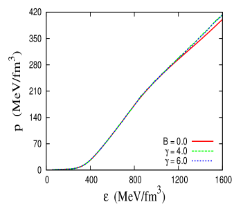
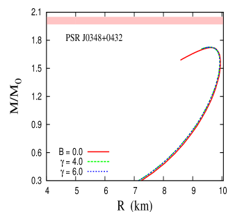
Figure 7: (Color online) EoS and mass-radius relation for a quark star with zero magnetic field and two variations of magnetars with the $G_{v}$ channel. No quark stars results agree with the PSR J0348+0432.

The results for the particle population are exactly the same as the ones obtained without the vector channel. This is due to the fact that all coupling constants are universal, coupling equally the three quarks. This result was already noted in ref. DebPRC2014 . Due to this fact, we do not plot the fraction os particles here, as it can be seen in Fig. (5).

In Fig. (7) we replot the EoS and the mass-radius relation for quark matter and magnetars with the vector channel. As the vector channel enters in the pressure calculation, causing the EoS to become stiffer we expect higher maximum masses as we show in Tab. 6. However, as we can see, the increase of the mass is not enough to reproduce the PSR J0348+0432 pulsar. In this work we use the parameters presented in ref. Kun2 , which were obtained from the fitting of the physical quantities shown in Tab. 4. With these physical quantities it is improbable that a NJL model be able to predict two solar masses quark stars, although this possibility is not completely ruled out. Another point worth mentioning is that we could have raised the maximum mass up to 2.0 solar masses by increasing the value of the $G_{v}$ coupling, as done in DebPRC2014 . However, instead of artificially increasing the vector channel, as it would violate LQCD results, we have chosen to face the consequences. The present study indicates that massive pulsars cannot be composed of deconfined quarks, at least if we believe that the NJL with the parametrization used in the present work is a reliable quark model. This does not completely rule out the possibility of quark stars. As pointed in ref. DebJCAP2019 and other references therein, the hadronic neutron star could be a metastable system, which eventually collapses. If the original neutron star had a mass beyond 1.74 $M_{\odot}$ it would become a black hole. However, a lower mass neutron star would become a quark star. The other possibility is that the metastable hadronic star can face a transition to a hybric star Melrose , an object with both, hadron and quark matter hybrid , as discussed in the next section.

$\gamma$	$M/M_{\odot}$	$R(km)$	$\epsilon_{c}$ ($MeV/fm^{3}$)	$B_{c}$ ($10^{18}G)$	$R_{1.4}(km)$
$B=0$	1.73	9.60	1521	0.0	9.89
4	1.74	9.57	1499	2.29	9.86
6	1.73	9.59	1478	2.10	9.86

Table 6: Quark stars main properties with the $G_{v}$ coupling. Even with this channel the maximum masses are not high enough to explain the massive PSR J0348+0432.

The effect of the magnetic field only increases the mass by 0.01$M_{\odot}$, as all other models investigated with the chaotic magnetic field approximation, i.e., the increase in the maximum mass is very subtle.

IV Magnetars as Hybrid Stars

As the density increases towards the star core, quarks become more energetically favorable than baryons, and ultimately the neutron star core may be composed of deconfined quarks. If the entire star does not convert itself into a quark star as suggested by the Bodimer-Witten conjecture, the final composition is a quark core surrounded by a hadronic layer. This is what is generally called a hybrid star. Nevertheless the nature of a hybrid star itself is not a closed question. Some authors, as Hans Beth, and Brian Serot Beth ; Serot2 claimed that the quark-hadron phase transition needs to be a constant-pressure phase transition obtained through a Maxwell construction. Within Maxwell constructions the quark and the hadron phases are spatially separated and there is a discontinuity in the electron chemical potential, although the nucleon chemical potentials are continuous. On the other hand Glenndening  Glen suggested that Maxwell construction is $\beta$ unstable at the interface between the phases and proposed a construction in which the pressure and all chemical potentials (including the electron chemical potential) are continuous, the one called Gibbs construction. Under these construction quarks and hadrons coexist in a mixed state, generating one intermediate phase in between the hadronic and the quark phases. Despite these differences, some authors  Chiba1 ; Chiba2 ; Paoli performed studies on hybrids stars with both, Maxwell and Gibbs construction. They all concluded that there is no significant difference on the macroscopic properties of the hybrid stars. Due to this fact, in this work we use a Maxwell construction, which is simpler. In this case we impose that the transition occurs when the pressure of the quark matter equals the pressure of the hadronic matter at the same chemical potential:

$$\mu^{H}_{n}=\mu^{Q}_{n}\quad\mbox{and}\quad p^{H}=p^{Q},$$ (28)

where the neutron chemical potential can be written in terms of the quark ones as:

$$\mu_{d}=\mu_{s}=\frac{1}{3}(\mu_{n}+\mu_{e})$$

$$\mu_{u}=\frac{1}{3}(\mu_{n}-2\mu_{e}).$$ (29)

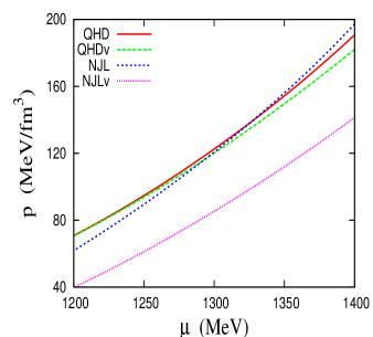
Figure 8: (Color online) Pressure as function of the chemical potential with (right) and without (left) magnetic field (B= $3\times 10^{18}$ G). If a hadronic EoS crosses a quark one, the phase with deconfined quarks becomes energetically favorable at higher densities.

We have previoulsy presented two possibilities to describe hadronic matter, with and without the vector channel (let’s call them QHD and QHDv respectively). We have also shown two ways to describe quark matter (NJL and NJLv). Moreover each possibility has been studied in two configurations of the magnetic field. Now we can study how each of these factor influences the formation of hybrid stars. To accomplish that, we plot in Fig. (8) the pressure as function of the chemical potential, and seek for the point that satisfies the conditions presented in Eq. (28) with and without magnetic field.

We see that the vector channel in the hadron phase increases the pressure, so it induces the hadron quark phase transition at early densities when compared with the case without the $\phi$ meson. On other hand, the vector channel in the quark phase increases the pressure as well. With the inclusion of these two vector channels, the pressure becomes higher in the quark phase than in the hadronic one, thus suppressing the phase transition. Indeed, if we believe that the NJLv model is a good model to describe quark matter, therefore it is not probable that hybrid stars exist since, as we can see, Eq. (28) is not satisfied.

More interesting phenomena, however, appear when we deal with the magnetic field. As pointed out during our discussions on hadronic and quark stars, the effect of the magnetic field on the EoS is not relevant, causing only a small increase on the maximum masses. However, when we seek for both phases crossing point we see that the magnetic field plays the role of suppressing the quark onset. As we can see from the study involving QHDv to NJL the chemical potential at the phase transition point is pushed away from 1295 $MeV$ to 1340 $MeV$. When QHD and NJL models are considered, the chemical potential moves from 1330 $MeV$ to 1439 $MeV$. Note that such high chemical potential is already above the one corresponding to the maximum mass of a hadronic neutron star. The fact that the magnetic field strongly difficults the formation of a hybrid star was already pointed out in the recent literature Dex4 ; Dex5 . Our study corroborates these results. The phase transition pressure and chemical potential values are presented in Tab. 7.

Hadron	Quark	B ($\times 10^{18}$) G	$\mu_{n}^{H}=\mu_{n}^{Q}$	$p^{H}=p^{Q}$	$\epsilon^{H}$ $(MeV/fm^{3})$	$\epsilon^{Q}$ $(MeV/fm^{3})$
QHD	NJL	0.0	1330 $MeV$	141 $(MeV/fm^{3})$	711	808
QHDv	NJL	0.0	1295 $MeV$	117 $(MeV/fm^{3})$	597	730
QHD	NJL	3.0	1439 $MeV$	264 $(MeV/fm^{3})$	1130	1409
QHDv	NJL	3.0	1340 $MeV$	149 $(MeV/fm^{3})$	683	834

Table 7: Chemical potential and pressure at phase transition for QHD to NJL with and without the vector channel and the magnetic field. We also present the energy density of each matter at the phase transition. The NJLv model does not allow a phase transition.

Figure 9: (Color online) EoS and mass-radius relation for models that allow a construction of an hybrid star.

As can be seen, there are three possible models of hybrid stars that we now nominate: model A corresponds to the EoS obtained from QHD and NJL without magnetic field, model B to QHDv and NJL also with no magnetic field, and finally model C to the QHDv to NJL with the inclusion of magnetic field. We plot the EoS and the mass-radius diagram for them in Fig. (9) and resume the main properties in Tab. 8.

Model	$M/M_{\odot}$	$R(km)$	$\epsilon_{c}$ ($MeV/fm^{3}$)	$M_{min}/M_{\odot}$	$R_{1.4}(km)$
A	1.93	12.88	877	1.91	13.63
B	1.94	13.04	822	1.92	13.63
C	2.02	12.97	879	2.00	13.58

Table 8: Hybrid star properties indicating that the allowed mass values for a quark core lie within a very narrow band.

The maximum mass of a hybrid neutron star without magnetic field lies just slightly below the lower limit of the PSR J0348+0432. When the magnetic field is included, we see that the PSR J0348+0432 mass constraint is satisfied. Notice that hybrid stars bear the lower value of the energy density at the core as compared with hadronic and quark stars, and thus lower values of the magnetic fields. Also they have the bigger radii for the maximum masses when compared with hadronic and quark stars. We also investigate the $M_{min}$, which is the minimum mass star that supports a quark core, i.e., stars with masses below $M_{min}$ are purely hadronic. We see that, although the existence of a hybrid star is possible, it is very unlikely, because there is just a narrow mass range that supports a quark core. Indeed if we move away from the maximum mass by only 0.02$M_{\odot}$ we obtain a pure hadronic star, instead of a hybrid one. This small range is even below the experimental uncertainty on the mass of the PSR J0348+0432. Hence, its true nature is still an open subject, although probably it is not a quark star.

V Final Remarks

In this work we studied the influence of a non standard repulsive channel and strong magnetic field in different classes of compact stars. The results can be summarized:

• The $\phi$ meson in the hadronic matter significantly increases the pressure, making hadronic neutron stars fully compatible with the PSR J0348+0432, and even with the more massive MSP J0740+6620. As this meson does not affect nuclear properties and brings no new parameters, since we can constrain $g_{\phi}$ with the help of symmetry group, its presence seems to improve the description of hadronic matter at high densities.

• The $G_{v}$ in the quark matter also increases the pressure. However there are two problems: First, unlike the hadronic case, this new vector channel cannot be fixed by theory, only by phenomenology. Second, although there is some consensus about the possible values of $G_{v}$ from lattice QCD, even with this term the quark stars are not massive enough to describe the PSR J0348+0432. An arbitrary increase of $G_{v}$ in order to accomplish that seems highly unphysical.

• As far as the chaotic magnetic field is concerned, some points are worth emphasizing: $1-)$ In our previous work Lopes2015 , we compared the effect of the chaotic magnetic field with those obtained by Lorene available at that date and obtained very similar results. $2-)$ The chaotic magnetic field restores the thermodynamic pressure. $3-)$ The chaotic magnetic field does not overestimate the neutron star mass as stated in previous works and also reproduced here.

• The magnetic field has very little influence on the macroscopic properties of hadron and quark stars, but its inclusion makes the formation of hybrid stars more difficult, pushing away the critical neutron chemical potential.

• The additional vector channel in QHD favors the existence of hybrid stars, while in NJL it suppresses this possibility completely.

• According to the model presented in this work, the minimum and the maximum masses of a hybrid star are very close to each other, indicating that only stars at the edge of mechanical stability can be hybrid stars. If they exist, hybrid stars are very rare in the universe, although the results are model dependent.

• Quark stars can still be present in nature, if the Bodmer-Witten conjecture is true. Low masses hadronic neutron stars can collapse to form a quark star. Massive neutron stars collapse into black holes.

• We can describe even more massive neutron stars if hyperons are not present. The hyperon puzzle is still open and can only be accounted for under special circumstances.

Moreover, it is worth noticing that the recent detection of gravitational waves from neutron stars merger has opened a new window to constrain dense nuclear matter LIGO . A clear correlation between dimensionless tidal deformability and the radius of the canonical star was found (see, for instance,malik ; Odilon1 ). Some studies zhao ; elias constrain the radii of the canonical stars to 12.00 km $<~{}R_{1.4}~{}<$ 13.45 km, while in malik , the proposed range is $11.82~{}\mbox{km}\leqslant R_{1.4}\leqslant 13.72~{}\mbox{km}$ and in Odilon2 it is $10.36~{}\mbox{km}\leqslant R_{1.4}\leqslant 12.55~{}\mbox{km}$. By using the neutron skin values as a new constraint, the upper limit for $R_{1.4}$ was set to be $13.76~{}\mbox{km}$ fatt18 . There is no direct evidence that the neutron stars in the binary system are magnetars, but anyway, our results in this work (around 13.6 km) are compatible with many of the constraints just mentioned.

Before finishing this work, as pointed out in the introduction, we discuss in more detail our results and the validity of the chaotic magnetic field approximation in the light of a new study published in ref. debi2018 concerning the magnetic field distribution in magnetar interiors. Using full relativistic numerical calculation, it was found that the magnetic field can be expressed as a multipolar expansion that accounts for the monopole contribution, the dipole term, the quadrupole and so on. Now, the important fact here is is that our study is based on the chaotic magnetic field formalism, which is a monopole approximation for the magnetic field profile. However as shown in Fig 3 of debi2018 the monopole term is dominant in almost the entire star. More than that, the monopole term is specially dominant in the neutron star core, when the magnetic field is stronger. So, in the limit of very high field, when its influence is bigger, our results are very close to those obtained in this work. Moreover, one of the main problems of using TOV equations in the presence of strong magnetic fields is the possible appearance of anisotropies in the momentum-energy tensor. As pointed out in ref. debi2018 in most cases, $T^{\theta\theta}~{}\neq~{}T^{rr}$. However, exactly due to the monopole nature of the chaotic magnetic field, we always obtain $T^{\theta\theta}=T^{rr}$, which guarantees that the TOV approximation is a good one in this case.

Acknowledgments

This work is a part of the project INCT-FNA Proc. No. 464898/2014-5 and it was partially supported by CNPq (Brazil) under grant 301155.2017-8 (D.P.M).

References

- (1) S. L. Shapiro, S. A. Teukolsky, Black Holes, White Dwarf and Neutron Stars , Wiley, New York, U.S.A. (1983)
- (2) C. Thompson and R. C. Duncan, Mon. Not. Roy. Astron. Soc. 275, 255 (1995)
- (3) C. Thompson and R. C. Duncan, Atrophys. J. 473, 322 (1996)
- (4) S. Mereghetti, Braz. J. Phys. 43, 356 (2013)
- (5) S.A. Olausen, V.M. Kaspi, The Astrophys. J. Supp. 212, 6 (2014)
- (6) B. D. Serot, Rep. Prog. Phys. 55, 1855 (1992)
- (7) R.C. Tolman, Phys. Rev. 55, 364 (1939); J. R. Oppenheimer, G. M. Volkoff, Phys. Rev. 33, 374 (1939).
- (8) Fortin et al, Phys.Rev. C 95, 065803 (2017)
- (9) Oertel et al, Eur.Phys.J. A52 (2016) 50
- (10) Chatterjee et al, Eur.Phys.J. A52 (2016) 29
- (11) N. K. Glendenning, Compact Stars,Springer, New York - Second Edition (2000)
- (12) L. L. Lopes, D.P. Menezes, Phys. Rev. C 89, 025805 (2014)
- (13) Negreiros et. al., Phys.Lett. B 718 (2013) 1176.
- (14) B. Franzon, V. Dexheimer, S. Schramm Mon. Not. Roy. Astr. Soc. 456, 2937 (2016)
- (15) D. Chatterjee et al, Mon. Not. R. Astron. Soc. 447, 3785 (2015).
- (16) E. Witten,Phys. Rev. D 30, 272 (1984)
- (17) A. R. Bodmer,Phys. Rev. D 4, 1601 (1971)
- (18) L. McLerran, R. D. Pisarski, Nucl. Phys. A 796, 83 (2007)
- (19) Y. Nambu, G. Jona-Lasinio, Phys. Rev. 122, 345 (1961)
- (20) D.P. Menezes et al., Phys. Rev. C 79, 035807 (2009)
- (21) D.P. Menezes et al., J. Cosm. Astrop. Phys. 01, 024 (2019)
- (22) L. L. Lopes, D.P. Menezes, Eur. Phys. J. A 52, 17 (2016)
- (23) R. Gomes, V. Dexheimer, S. Han, S. Schramm Mon. Not. R. Astr. Soc. 485,4873 (2019)
- (24) S. Lalit et al., Eur. Phys. J. A 55, 10 (2019)
- (25) U. Lee Mon. Not. R. Astr. Soc. 476,3399 (2018)
- (26) M. Gusakov, E. Kantor, and D. Ofengeim Phys. Rev. D 96, 103012 (2017)
- (27) R. Gomes, et al., Astron. Astrophys. 627, A61 (2019)
- (28) R. Gomes, V. Dexheimer, S. Schramm Phys. Rev. D 94 044018 (2016)
- (29) R. Gomes, et al., Astrophys.J 850, 20 (2017)
- (30) M. Mariani Mon. Not. R. Astron. Soc. 489, 4261 (2019)
- (31) Ya. B. Zel’dovich, I. D. Nivikov Stars and Relativity , Dover, New York, U.S.A. (1996)
- (32) L. Lopes and D. P. Menezes, J. Cosm. Astrop. Phys. 08, 002 (2015)
- (33) F. Wu, C. Wu and Z.Z. Ren, Chin. Phys. C 41, 045102 (2017)
- (34) R. Blandford and L. Hernquist, J. Phys. C 15, 6233 (1982)
- (35) Debarati Chatterjee, Jerome Novak and Micaela Oertel, Phys. Rev. C 99, 055811 (2019)
- (36) R. Cavagnoli, D. P. Menezes, C. Providencia, Phys. Rev. C 84, 065810 (2011).
- (37) L. L. Lopes, D.P. Menezes, Braz. J. Phys. 44, 744 (2014)
- (38) M. B. Tsang et al, Phys. Rev. C 86, 015803 (2012)
- (39) M. Oertel et al, Rev. Mod. Phys. 89, 015007 (2017).
- (40) Lattimer & Steiner, Eur. Phys. J. A 50, 40 (2014)
- (41) H. Pais & C. Providencia, Phys.Rev. C 94, 015808 (2016)
- (42) V. Dexheimer et al, J.Phys. G 46, 034002 (2019)
- (43) Providencia et al, Front. Astron. Space Sci., 26 March 2019
- (44) J. Boguta and A.R. Bodmer, Nucl. Phys. A 292, 413 (1977).
- (45) N. K. Glendenning, S. A. Moszkowski, Phys. Rev. Lett. 67, 2414 - (1991).
- (46) M. Dutra et al, Phys. Rev. C 90, 055203 (2014).
- (47) A. Pais, Rev. Mod. Phys. 38, 215 (1966)
- (48) L. L. Lopes, D.P. Menezes, Braz. J. Phys. 42, 428 (2012)
- (49) S. Pal, D. Bandyopadhyay, S. Chakrabarty, Phys. Rev. Lett. 78, 2898 (1997)
- (50) Q. Peng, H. Tong, Mon. Not. R. Astron. Soc. 378, 159 (2007)
- (51) Rhabi et al, J.Phys. G36 (2009) 115204
- (52) W. Greiner, L. Neise, H. Stocker, Thermodynamics and Statistical Mechanics, Springer, New York, (1995)
- (53) C.W. Misner, K.S. Thorne and J.A. Wheeler, Gravitation, Freeman and Company, San Francisco, U.S.A. (1973)
- (54) C.Y. Ryu, K.S. Kim and M.-K. Cheoun, Phys. Rev. C 82, 025804, (2010)
- (55) A. Rabhi, P.K. Panda and C. Providencia, Phys. Rev. C 84, 035803, (2011)
- (56) R. Mallick and M. Sinha, Mon. Not. R. Astron. Soc. 414, 159 (2011)
- (57) V. Dexheimer, R. Negreiros, S. Schramm, Eur. Phys. J. A 48 189, (2012)
- (58) R. Casali, L.B. Castro and D.P. Menezes, Phys. Rev. C 89, 015805 (2014)
- (59) R.O. Gomes, V. Dexheimer and C.A.Z. Vasconcellos, Astron. Nachr. 335 666, (2014)
- (60) V. Dexheimer, D.P. Menezes and M. Strickland, J. Phys. G 41 015203, (2014)
- (61) R. Mallick and S. Schramm, Phys. Rev. C 89, 045805 (2014)
- (62) O. Zubairi, F. Weber, J.Phys.Conf.Ser. 845, 012005 (2017)
- (63) M. Paret et al, Res.Astron.Astrophys. 15, 975 (2015)
- (64) G.E. Wright, Mon. Not. Roy. Astron. Soc. 162, 339 (1973)
- (65) P. Markey and R.J. Tayler, Mon. Not. Roy. Astron. Soc. 163, 77 (1973)
- (66) D. P. Menezes and M. D. Alloy, arXiv:1607.07687 (2016).
- (67) J. Antoniadis et al: Science 340, 1233232 (2013)
- (68) H. Cromartie et al: Nat. Astr. (2019) DOI: 10.1038/s41550-019-0880-2
- (69) C. Mota et al: arXiv:1911.03208
- (70) K. Hebeler et al, Phys. Rev. Lett. 105, 161102 (2010)
- (71) J.M. Lattimer and A.W. Steiner, Astrophys. J. 784, 123 (2014)
- (72) J. Ellis, J. I. Kapusta, K. A. Olive Nucl. Phys. B 348, 345 (1991)
- (73) L. Lopes and D. P. Menezes, J. Cosm. Astrop. Phys. 05, 038 (2018)
- (74) D. P. Menezes et al., Phys. Rev. C 80, 065805 (2009)
- (75) D. P. Menezes et al., Phys. Rev. C 89, 055207 (2014)
- (76) T Hatsuda, T. Kunihiro, Phys. Lett. B 198, 126 (1987)
- (77) T Hatsuda, T. Kunihiro, Phys. Rep. 247, 221 (1994)
- (78) R. Denke, M. B. Pinto, Phys. Rev. D 88, 056008 (2013)
- (79) M. Buballa and M. Oertel, Phys. Lett. B 457 (1999) 261.
- (80) V. Dexheimer, J.R. Torres and D.P. Menezes, Eur. Phys. J. C 73 (2013) 2569.
- (81) M. Kitazawa et al., Prog. Theor. Phys. 108, 5 (2002)
- (82) T. Klahn, T. Fischer, Astrophys.J. 810, 134 (2015)
- (83) M. Hanauske et al., Phys. Rev. D 64, 043005 (2001)
- (84) G. Y. Shao et al., Phys. Rev. D 85, 114017 (2012)
- (85) G. A. Contrera, A. G. Grunfeld, D. B. Blaschke., Phys. Part. Nucl. Lett. 11, 4 (2014)
- (86) K. Kashiwa, T. Hell, W. Weise, Phys. Rev. D 84, 056010 (2011)
- (87) J. Sugano et al., Phys. Rev. D 90, 037901 (2014)
- (88) D. P. Menezes, D. B. Melrose, C. Providência, and K. Wu, Phys. Rev. C 73, 025806 (2006).
- (89) D. P. Menezes and C. Providência, Phys. Rev. C 68, 035804 (2003).
- (90) H. Beth, G. E. Brown, J. Cooperstein Nucl. Phys. A 462, 791 (1987)
- (91) B. Serot, H. Uechi Ann. Phys. A 179, 272 (1987)
- (92) T. Maruyama et al., Phys. Rev. D 76, 123015 (2007)
- (93) T. Maruyama et al., Phys. Lett. B 659, 192 (2007)
- (94) M. Paoli, D.P. Menezes, Eur. Phys. J. A 46, 413 (2010)
- (95) B. P. Abbott et al. (LIGO Scientific Collaboration and Virgo Collaboration), Phys. Rev. Lett. 119, 161101 (2017).
- (96) Tuhin Malik, N. Alam, M. Fortin, C. Providência, B. K. Agrawal, T. K. Jha, Bharat Kumar, and S. K. Patra Phys. Rev. C. 98, 035804 (2018).
- (97) Odilon Lourenço, Mariana Dutra, César H. Lenzi, César V. Flores, and Débora P. Menezes, Phys. Rev. C 99, 045202 (2019).
- (98) T. Zhao & J. Lattimer, Phys.Rev. D bf 98, 063020 (2018)
- (99) E. Most et al., Phys.Rev. Lett. 120, 261103 (2018)
- (100) Odilon Lourenço, Mariana Dutra, César Lenzi, S. K. Biswal, M. Bhuyan, Débora P. Menezes, arXiv: 1901.04529, Eur. Phys. Jour. A (2020) in press.
- (101) F. J. Fattoyev, J. Piekarewicz and C. J. Horowitz, Phys. Rev. Lett. 120, 172702 (2018).