Empirical inference on the Majorana mass of the ordinary neutrinos

Abstract

There is a broad theoretical consensus on the idea that ordinary neutrinos have a Majorana mass, but we have no clear prediction about its value, and direct experimental measurements of this quantity are rather challenging. In this work, we argue that the current cosmological measurements allow us to obtain precise information on the effective Majorana mass, i. e. the electronic-type mass of ordinary neutrinos. We show that the numerical results that we obtain can be accurately reproduced, and hence tested, by a straightforward analytical procedure. We then discuss the stability of the assumptions at the basis of our analysis and the implications of our findings for neutrinoless double beta decay.
Published on: Phys. Rev. D 100, 073003 (2019)

I Introduction

There is compelling evidence from oscillation phenomena Fukuda et al. (1998); Ahmad et al. (2002); Eguchi et al. (2003); Michael et al. (2006); Agafonova et al. (2015) that ordinary neutrinos are not massless. However, we do not have empirical knowledge of the absolute values of these masses. Nor do we know whether these are of Dirac type — as for all charged fermions — or of Majorana type.

A Majorana nature for the neutrino mass is considered quite natural from the theoretical point of view Minkowski (1977); Yanagida (1979); Gell-Mann et al. (1979); Mohapatra and Senjanovic (1980). This hypothesis could be experimentally tested via the observation of neutrinoless double beta decay ($0\nu\beta\beta$), the transition $(A,Z)\to(A,Z+2)+2\text{e}^{-}$ where a nucleus increases its charge by two units, emitting two electrons but no neutrinos Furry (1939).

The rate of $0\nu\beta\beta$ depends quadratically upon a combination of the neutrino masses $m_{i}$, the mixing matrix $U_{\text{e}i}$ and the Majorana phases, which is called the “effective Majorana mass” and, within the three-ordinary-neutrino framework, is defined as

$$m_{\beta\beta}\equiv\left|\sum_{i=1,2,3}m_{i}\left|U_{\text{e}i}^{2}\right|e^{i\xi_{i}}\right|.$$ (1)

A key issue is therefore to understand which is the actual value of $m_{\beta\beta}$.

The theory of fermion masses is not yet sufficiently developed to give definitive answers. For instance, it has been argued that a plausible value for $m_{\beta\beta}$ could be of the order of $m\cdot\theta_{\mathrm{C}}^{n}$, where $\theta_{\mathrm{C}}\simeq 13^{\circ}$ is the Cabibbo mixing angle, $m\equiv\sqrt{\Delta m^{2}_{\mathrm{atm}}}\simeq 50\,\text{meV}$ and $n=1,2$ Vissani (1998); Dell’Oro et al. (2018). Still, these indications only offer an “educated guess” pointing towards the $\mathcal{O}(1\,\text{meV})$ scale and might be correct within a factor of a few, which practically means that we do not know $m_{\beta\beta}$ reliably. Principled models, on the other hand, such as $SO(10)$ theories, offer more convincing explanations for light Majorana neutrino masses. However, these motivations have been extensively investigated Matsuda et al. (2002); Bajc et al. (2006); Bertolini et al. (2009); Joshipura and Patel (2011); Abud et al. (2012); Altarelli and Meloni (2013); Dueck and Rodejohann (2013); Ohlsson and Pernow (2019), but they remain far from being unique and we lack clear criteria on how to assess them.

In this situation, it seems reasonable to fully exploit the information coming from the experimental observations in order to try to quantify $m_{\beta\beta}$. Neutrino oscillations are a powerful tool in this regard, and the mixing angles and mass splittings are currently measured quite precisely Capozzi et al. (2018); de Salas et al. (2018); Esteban et al. (2019). In particular, the interpretation of the oscillation phenomena is beginning to prefer the so-called normal hierarchy (NH) over the inverted hierarchy (IH) for the neutrino mass spectrum, now at a level greater than $3\sigma$ (see the Appendix). However, neutrino oscillations only measure the differences between the neutrino mass eigenstates $m_{i}^{2}-m_{j}^{2}$ and not the absolute masses.

The most relevant information on absolute masses to date comes from cosmological measurements. It is fair to state that a cautious approach is highly advisable while dealing with the results from cosmological surveys, due to the crucial role of the theoretical assumptions in building the specific model. On the other hand, this cannot provide an excuse in order to ignore a whole category of results. Cosmology is able to probe the value of the sum of the active neutrinos that, consistently with the hypothesis of three light neutrinos, is defined as $\Sigma\equiv m_{1}+m_{2}+m_{3}$. Very stringent upper limits $\Sigma<180\,\text{meV}$ at the $2\sigma$ C. L. have been obtained by many independent analyses Ade et al. (2016); Palanque-Delabrouille et al. (2015); Di Valentino et al. (2016); Zhang (2016); Cuesta et al. (2016); Giusarma et al. (2016); Yèche et al. (2017); Aghanim et al. (2018); Roy Choudhury and Hannestad (2019).

In a previous work, we showed the importance of the combination of the results of post-2015 Planck observations and “small scale” cosmology measurements for $0\nu\beta\beta$ Dell’Oro et al. (2015). Here, we demonstrate how to obtain detailed information on $m_{\beta\beta}$, possibly measuring this important parameter. We first describe a direct Monte Carlo procedure to derive the likelihood of $m_{\beta\beta}$ from that of $\Sigma$ in Sec. II. In Sec. III, we test the results we obtain by means of an analytical calculation. Finally, in Sec. IV, we critically discuss the assumptions underlying the present analysis and examine the implications of the predictions we obtain for $0\nu\beta\beta$. The main results of this work are summarized in Figs. 1 and 2, that are discussed in Secs. II and III.

II Distribution of $m_{\beta\beta}$ from data

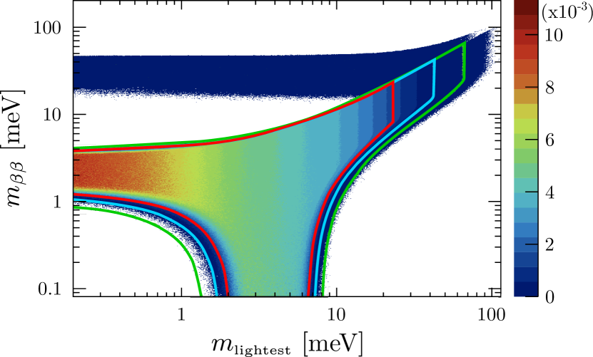
FIG. 1: Density plot of $m_{\beta\beta}$ as a function of $m_{\mathrm{lightest}}$ as a result of the Monte Carlo simulation. The two regions correspond to the NH and IH cases. For each event, the mass hierarchy is chosen according to the preference evidenced in Ref. Capozzi et al. (2018). The red, blue and green contours are the 1$\sigma$, 2$\sigma$ and 3$\sigma$ C. L. intervals.

In a frequentist approach, one would assume each value of $m_{\beta\beta}$ lying below the current experimental bound to be equally allowed. In the case of NH, this would imply the impossibility of excluding that this parameter is actually negligibly small. However, this is not necessarily the case. In fact, it is possible to obtain useful information on $m_{\beta\beta}$ independently of that coming from the direct experimental search for $0\nu\beta\beta$.

As an illustrative case, let us suppose that one day cosmology will be able to measure a value of $\Sigma$, and that its value will turn out to be one of the current $2\sigma$ upper limits, i. e. $140\,\text{meV}$ Yèche et al. (2017). Since the mass splittings are reliably known, the lightest neutrino mass would be set to $38\,\text{meV}$. In turn, still assuming that the neutrinos have a Majorana mass, we could conclude that $m_{\beta\beta}$ lies in the range $(13-39)\,\text{meV}$. In particular, the possibility that $m_{\beta\beta}=0$ would be excluded for experimental reasons.

Passing to a more realistic case, today we can dispose of a limit $\Sigma$ from cosmology, but not a measurement. Still, the range of allowed values of $m_{\beta\beta}$ (for a given $\Sigma$) can only be explored by declaring a prior distribution for some relevant parameter — that is, by adopting a Bayesian approach.

A prediction for the possible value of $m_{\beta\beta}$ can by obtained by simulating a large series of combinations of neutrino mass parameters, starting from the information available today. We thus developed a Monte Carlo tool that iteratively extracts values of $m_{\beta\beta}$ by providing as input randomly generated values of the mass splittings and mixing angles, and of $\Sigma$. The former are picked around the best-fit values of the global analysis of Ref. Capozzi et al. (2018) assuming Gaussian errors. The latter parameter is selected within the limit reported in Ref. Yèche et al. (2017), in which the authors obtained an almost Gaussian likelihood (see Fig. 10 in the reference) that can be approximated by the expression:

$$G(\Sigma)=\frac{1}{45.4\,\text{meV}}\,\exp\left[-\frac{1}{2}\frac{(\Sigma-41.3\,\text{meV})^{2}}{(49.7\,\text{meV})^{2}}\right].$$ (2)

Indeed, starting from $G(\Sigma)$ of Eq. (2), we are able to reproduce the same limit $\Sigma<140\,\text{meV}$ at the $2\sigma$ C. L.  reported in the reference.

For each event that we simulate, the hierarchy scenario (NH or IH) is initially selected with a preference for NH, according to the result of the analysis of Ref. Capozzi et al. (2018). A value for the lightest neutrino mass, $m_{\mathrm{lightest}}$, is then calculated starting from $\Sigma$ and the mass splittings Dell’Oro et al. (2016). When $m_{\mathrm{lightest}}$ is negative, i. e. it falls outside the physical range, the event is rejected and a new one is generated. The allowed interval for $m_{\beta\beta}$ is fixed once $m_{\mathrm{lightest}}$ is known and it is comprised within the extremes Vissani (1999)

$$m_{\beta\beta}^{\max}=\sum_{i=1}^{3}\bigl{|}U_{ei}^{2}\bigr{|}m_{i},$$ (3a)

$$m_{\beta\beta}^{\min}=\max\Bigl{\{}2\bigl{|}U_{ei}^{2}\bigr{|}m_{i}-m_{\beta\beta}^{\max},0\Bigr{\}}\quad i=1,2,3.$$ (3b)

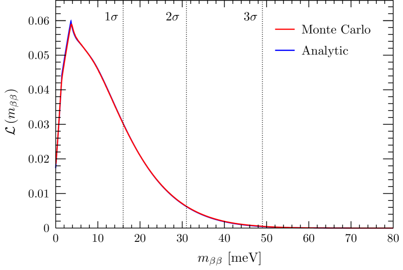
FIG. 2: Differential distributions of $m_{\beta\beta}$ obtained by projecting the density plot of Fig. 1 (red line) and as a result of the analytic procedure discussed in the text (blue line). The 1$\sigma$, 2$\sigma$ and 3$\sigma$ C. L. intervals are reported.

The value of $m_{\beta\beta}$ is randomly selected within this range with flat probability. In principle, other solutions are possible. One could adopt the most pessimistic attitude, by setting $m_{\beta\beta}=m_{\beta\beta}^{\min}$ or, on the contrary, the most optimistic view, by setting $m_{\beta\beta}=m_{\beta\beta}^{\max}$. These two extreme choices for the prior of $m_{\beta\beta}$ could be of some interest in order to assess the chances of failure or success in the search for $0\nu\beta\beta$. However, neither of them is particularly supported by existing theoretical considerations. Also, since our primary goals are to illustrate an analysis methodology and to obtain reasonable expectations on $m_{\beta\beta}$, we did not consider these options. A valid alternative, that has already been used in the literature, is to take random Majorana phase uniformly distributed in $[0;2\pi)$ and to construct $m_{\beta\beta}$ accordingly Benato (2015); Caldwell et al. (2017); Agostini et al. (2017). In this latter case, one typically expects larger values for $m_{\beta\beta}$ up to $\sim 10\%$ since there is a larger probability that the two phases will add constructively, rather than destructively (Fig. 3). This situation is more conducive to the experimental searches. However, from a theoretical point of view, it seems easier to motivate a preference for a flat prior on $m_{\beta\beta}$, since this quantity is more directly connected to the Majorana mass term of the Lagrangian density, and thus we opted for this choice.

The result of the simulation is shown in Fig. 1. In total, one billion events have been generated. The contour lines at different C. L. are drawn by “cutting” the distribution on the $(m_{\mathrm{lightest}}:m_{\beta\beta})$ plane at fixed ratios of the fraction of surviving events over the total one. The IH region is interested by no 1, 2, 3$\sigma$ contour lines since this scenario is excluded at more than $3\sigma$ by the oscillation studies. The tight limits on $\Sigma$ push towards smaller values of $m_{\mathrm{lightest}}$ and this in turn favors smaller values of $m_{\beta\beta}$. This appears even more clearly by projecting the plot onto the $m_{\beta\beta}$ axis (Fig. 2). These results will be further discussed in the following sections.

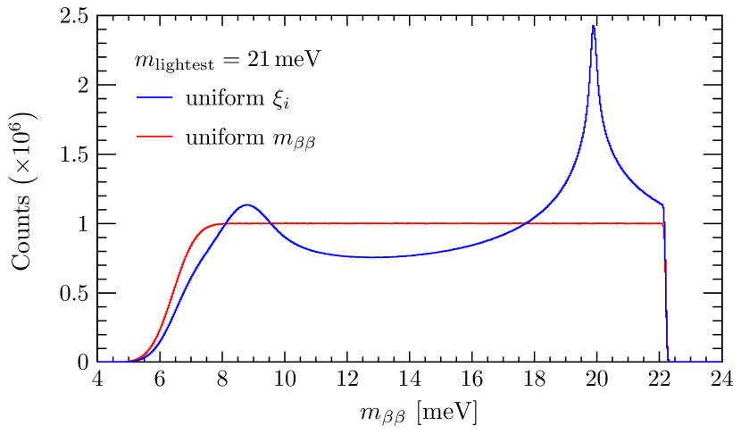
FIG. 3: Event distribution for a fixed value of $m_{\mathrm{lightest}}$ (assuming the NH scenario). Random mass splittings and mixing angles have been picked around the best-fit values from Ref. Capozzi et al. (2018) assuming Gaussian errors, thus fixing the allowed range for $m_{\beta\beta}$. Then, two values for $m_{\beta\beta}$ have been extracted assuming a uniform distribution for either $m_{\beta\beta}$ (red) or the Majorana phases (blue). The Gaussian shape of the distributions at the boundaries is due to the Gaussian errors on the oscillation parameters.

III Analytic test of the results

In order to test our Monte Carlo tool, we developed an analytic procedure that allowed us to obtain a distribution of $m_{\beta\beta}$ to be compared to that derived in the previous section (see in particular Fig. 2). We focused on the NH scenario, so that the lightest $m_{i}$ is now $m_{1}$ (recall Eq. (1)).

As a starting point, let us consider a priori a flat distribution for each fixed $m_{1}$, namely

$$d\mathcal{L}^{\mathrm{prior}}\left(m_{\beta\beta}\right)=\frac{dm_{\beta\beta}}{m_{\beta\beta}^{\max}(m_{1})-m_{\beta\beta}^{\min}(m_{1})}$$ (4)

where the extremes have the known expressions reported in Eqs. (3a)–(3b). As previously stated, we assume a uniform distribution for $m_{\beta\beta}$ within the allowed range. The information on the distribution of $m_{1}$ required by Eq.(4) can be extracted from cosmology. The constraints on $\Sigma$ can be summarized by the likelihood

$$d\mathcal{L}(\Sigma\,|\,\text{cosm})=G(\Sigma)\,d\Sigma$$ (5)

where we can consider $\Sigma$ as a function of $m_{1}$. We use the expression in Eq. (2) and compute the normalization by integrating $G(\Sigma)$ down to $\Sigma=58.5\,\text{meV}$, corresponding to the case $m_{1}=0$, given the present values of the mass splittings Capozzi et al. (2018). We thus obtain

$$d\mathcal{L}(m_{1}\,|\,\text{cosm})=G(\Sigma)\ \frac{d\Sigma}{dm_{1}}\ dm_{1}=E(m_{1})\,dm_{1}.$$ (6)

The distribution of the lightest neutrino mass $E(m_{1})$ is shown in Fig. 4. The curve has a maximum around $m_{1}=10$ meV since the Jacobian $d\Sigma/dm_{1}$, which is a strictly increasing function, disfavors the values close to $m_{1}=0$, while the likelihood extracted from Ref. Yèche et al. (2017) does the opposite.

It is worth noticing that the propagation of the uncertainties on the mass splitting values introduces a variation in the distribution $E(m_{1})$. However these are of the order of a few parts per 10,000. Therefore, we can neglect them.

The bidimensional distribution of $m_{\beta\beta}$ and $m_{1}$, which is automatically normalized, is then

$$\begin{split}d\mathcal{L}(m_{\beta\beta},m_{1})=\ &d\mathcal{L}^{\mathrm{prior}}(m_{\beta\beta})\times d\mathcal{L}(m_{1}\,|\,\text{cosm})\\[5.0pt] &=H(m_{1})\ dm_{\beta\beta}\ dm_{1}\end{split}$$ (7)

where

$$H(m_{1})=\frac{E(m_{1})}{m_{\beta\beta}^{\max}(m_{1})-m_{\beta\beta}^{\min}(m_{1})}.$$ (8)

By integrating over all the possible values of $m_{1}$, we get the posterior distribution of $m_{\beta\beta}$, which includes the information extracted from cosmology:

$$\begin{split}d\mathcal{L}^{\mathrm{posterior}}&(m_{\beta\beta})\equiv d\mathcal{L}(m_{\beta\beta}\,|\,\text{cosm})\\[5.0pt] &=F(m_{\beta\beta})\ dm_{\beta\beta}\end{split}$$ (9)

where

$$F(m_{\beta\beta})=\int_{m_{1}^{\min}(m_{\beta\beta})}^{m_{1}^{\max}(m_{\beta\beta})}H(m_{1})\ dm_{1}.$$ (10)

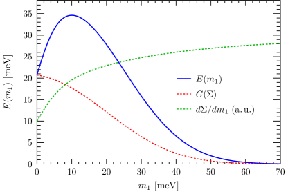
FIG. 4: Distribution of the lightest neutrino mass given the information from cosmology $G(\Sigma)$. The decreasing trend at small values of $m_{1}$ is due to the Jacobian $d\Sigma/dm_{1}$.

The functions describing the extreme values of $m_{1}$ given $m_{\beta\beta}$ can be analytically computed, since they correspond to solvable fourth-degree equations. The allowed region in the $(m_{1}:m_{\beta\beta})$ plane is that shown in Fig. 1, keeping in mind that we are now considering $m_{\beta\beta}$ as the independent variable.

The double integral we need to solve in order to get the probability of a specific $m_{\beta\beta}^{*}$, i. e. the cumulant distribution $\mathcal{L}(m_{\beta\beta}^{*})\equiv\mathcal{L}(m_{\beta\beta}<m_{\beta\beta}^{*})$, can actually be rearranged into a one-dimensional one:

$$\mathcal{L}(m_{\beta\beta}^{*})= \int_{\text{lower}(m_{\beta\beta}^{*})}^{\text{upper}(m_{\beta\beta}^{*})}E(m_{1})\,dm_{1}$$ (11)

$$\cdot\frac{\min\left[m_{\beta\beta}^{\max}(m_{1}),m_{\beta\beta}^{*}\right]-m_{\beta\beta}^{\min}(m_{1})}{m_{\beta\beta}^{\max}(m_{1})-m_{\beta\beta}^{\min}(m_{1})}.$$

The upper limit of integration is

$$\text{upper}(m_{\beta\beta}^{*})=m_{1}^{\max}(m_{\beta\beta}^{*})$$ (12)

while we can identify two cases for the inferior one, depending on the value of $m_{\beta\beta}^{*}$ with respect to $m_{\beta\beta,0}^{\min}\equiv m_{\beta\beta}^{\min}(m_{1}=0)$, namely

$$\text{lower}(m_{\beta\beta}^{*})=\left\{\begin{array}[]{ll}m_{1}^{\min}(m_{\beta\beta}^{*})&\mbox{ if }m_{\beta\beta}^{*}<m_{\beta\beta,0}^{\min}\\[5.0pt] 0&\mbox{ if }m_{\beta\beta}^{*}>m_{\beta\beta,0}^{\min}\end{array}\right..$$ (13)

If $m_{\beta\beta}^{*}\to 0$, then $\min\left[m_{\beta\beta}^{\max}(m_{1}),m_{\beta\beta}^{*}\right]=m_{\beta\beta}^{*}$ and the numerator $\to 0$. Instead, if $m_{\beta\beta}^{*}\to\infty$, then $\min\left[m_{\beta\beta}^{\max}(m_{1}),m_{\beta\beta}^{*}\right]=m_{\beta\beta}^{\max}(m_{1})$, the fraction approaches $1$, the inferior integration limit becomes $0$, and the integral of $E(m_{1})$ over all values is indeed $1$. In practice, for sufficiently high confidence levels (corresponding to larger values of $m_{\beta\beta}^{*}$), we will refer to the latter value of Eq. (13). Therefore, we can rewrite

$$\mathcal{L} (m_{\beta\beta}^{*})=\int_{0}^{m_{1}^{\min}(m_{\beta\beta}^{*})}E(m_{1})\,dm_{1}$$ (14)

$$+\int_{m_{1}^{\min}(m_{\beta\beta}^{*})}^{m_{1}^{\max}(m_{\beta\beta}^{*})}\frac{m_{\beta\beta}^{*}-m_{\beta\beta}^{\min}(m_{1})}{m_{\beta\beta}^{\max}(m_{1})-m_{\beta\beta}^{\min}(m_{1})}\,E(m_{1})\,dm_{1}.$$

By using Eq. (14), we can compute $m_{\beta\beta}$ for each given confidence level by setting $\mathcal{L}(m_{\beta\beta}^{*})=$ C. L. and choosing the oscillation parameters at their central (best-fit) values.

The value of $m_{\beta\beta}$ shifts when we include the variation on the mixing angles and mass splittings, since these enter both the integration limits and the integrand of Eq. (14). The individual contribution associated to the uncertainty of each oscillation parameter $x_{i}$ can be analytically computed. For a fixed confidence level, we get:

$$\Delta m_{\beta\beta,x_{i}}^{*}=\Delta x_{i}\,\frac{\partial\mathcal{L}(m_{\beta\beta}^{*})}{\partial x_{i}}\ \left|\frac{\partial\mathcal{L}(m_{\beta\beta}^{*})}{\partial m_{\beta\beta}^{*}}\right|^{-1}$$ (15)

evaluated in the best-fit central region. In practice, the overall effect is numerically small and the impact is negligible for our purposes.

In order check the consistency between the two described procedures, we can compare the resulting differential distributions for $m_{\beta\beta}$. The distribution from the likelihood of Eq. (9) can directly be compared with that obtained by the Monte Carlo simulation. The result, illustrated in Fig. 2, shows a very good agreement between the two procedures. This is a rather interesting conclusion: on the one hand, we have validated the numerical results. On the other hand, we have learned that the analytical method described here produces accurate results.

IV Discussion

The sum of the active neutrino mass coming from cosmology is a key ingredient of the analysis we presented. Therefore, we would like to begin our discussion with some considerations on the robustness of the current measurement of $\Sigma$.

To this extent, a first issue to address is the possible existence of additional light neutrinos, beyond those envisaged by the Standard Model. The presence of new neutral fermions was proposed a long time ago Pontecorvo (1958). Despite the fact that the values of their masses and mixing with the known neutrinos are a priori unknown, the interpretation of some experiments, when individually taken, would be compatible with the existence of neutrinos with mass of $\mathcal{O}(1\,\text{eV})$. These neutrinos would give rise to observable oscillation effects. On the other hand, the various analyses that have extensively considered the implications of this hypothesis highlighted the difficulties that arise, and even the inconsistencies, when compared to the available data Cirelli et al. (2005); Dentler et al. (2018). Therefore, while this could lead to more complicated scenarios for these new neutrinos Diaz et al. (2019), the “minimal” hypothesis of three ordinary neutrinos considered here is not weakened.

Recently, new results on the Hubble constant in the local Universe motivated the idea of rethinking the accepted cosmological model Riess et al. (2019). In principle, this could have an impact on the conclusions of our work. The new observations would be explained by the presence of some “kind” of sterile neutrinos. These neutrinos should have some specific proprieties, namely they should self-interact via strong interactions Verde et al. (2019) and should have rather small masses, subject to the stringent limits of cosmology Aghanim et al. (2018). In other words, while the assumption that there are three active neutrinos in cosmology could be reconsidered, we do not have any evidence that the measurement of $\Sigma$ should be affected. These considerations can be quantified by an example. Such a type of neutrino, with mass $m_{0}$ slightly larger than $m_{1}$, had already been introduced, not only to increase the number of effective neutrinos in cosmology, but also to explain certain features of the observed solar neutrino spectrum de Holanda and Smirnov (2011). The resulting mixing $U_{\text{e}0}^{2}\sim 10^{-3}$ and mass splitting $m_{0}^{2}-m_{1}^{2}\sim 0.2\ \Delta m^{2}_{\odot}$ de Holanda and Smirnov (2011) would add a contribution $U_{\text{e}0}^{2}(m_{0}-m_{1})$ to $m_{\beta\beta}$ of the order of $10^{-3}$ meV at most, and therefore it is completely negligible.

In summary, it seems premature to us to conclude that the the minimal set of assumptions adopted here and the reported results should require significant corrections.

To conclude our discussion, we would like to consider the implications of our findings for $0\nu\beta\beta$. Possible predictions for the expected value of $m_{\beta\beta}$ could be of great interest for the experimental community of $0\nu\beta\beta$ in helping to understand the chances for a positive observation, or to figure out how far from reach a promising target might be.

The current $0\nu\beta\beta$ experiments have already set limits of the order of $(10^{25}-10^{26})$ yr on the decay half-life Alvis et al. (2019); Agostini et al. (2018); Alduino et al. (2018); Anton et al. (2019); Gando et al. (2016). The corresponding upper bounds for $m_{\beta\beta}$ are around $100$ meV, with values that actually span a large range, mostly due to the theoretical uncertainties coming from nuclear physics Dell’Oro et al. (2014), which is a fundamental ingredient in order to extract the information on the neutrino mass. At the same time, the forthcoming generation of experiments is setting very ambitious goals, aiming at sensitivities greater than $10^{27}$ yr. This should allow to explore the parameter space of $m_{\beta\beta}$ of the order of tens of meV Agostini et al. (2017).

Given the present and near-future experiment sensitivities, we can thus analyze the results shown in Fig. 2. The differential distribution of $m_{\beta\beta}$ is peaked at $4\,\text{meV}$, while the $1\sigma$, $2\sigma$ and $3\sigma$ intervals extends up to 16, 31 and 49 meV, respectively. On the one hand, this means that we should be able to begin to probe the parameter region of interest in the coming years. On the other hand, this means that we are still quite far from fully exploring the “core” of the distribution, i. e. values of $m_{\beta\beta}$ of the order of a few meV. This ultimate investigation would require an extremely challenging multi-tonne experiment Biller (2013), but this hypothesis should not be ruled out.

The search for $0\nu\beta\beta$ remains one of the main ways, if not the only one, to address some major open questions in particle physics: the conservation of the lepton number conservation, and the value of the neutrino mass and its nature!

V Summary

We developed a Monte Carlo tool to extract the information on the effective Majorana mass starting from the available data on the neutrino masses, coming from the oscillation studies and from cosmology. We found that the distribution of $m_{\beta\beta}$ tends toward low values of the parameter region, with a mode at $4\,\text{meV}$, and a $3\sigma$ interval extended up to almost 50 meV. We validated our results with an analytical procedure, whose outcome perfectly matches the numerical one. Finally, we discussed the assumptions at the basis of our analysis and implications of the new information for neutrinoless double beta decay.

*

APPENDIX A On the preference for the Normal Hierarchy

In the global analyses, it is customary to present the preference for the hierarchy scenario in terms of the difference $\Delta\chi^{2}\equiv\chi^{2}_{\mathrm{IH}}-\chi^{2}_{\mathrm{NH}}>0$ between the two cases. This quantity has a different meaning than in the case of one-dimensional parameters. In order to determine how much is NH preferred by the data, we can estimate the likelihood

$$\begin{split}\mathcal{L}(\mbox{IH})&=\frac{\mathcal{L}^{\mathrm{cosm}}_{\mathrm{IH}}\times\text{e}^{-\chi^{2}_{\mathrm{IH}}}}{\mathcal{L}^{\mathrm{cosm}}_{\mathrm{IH}}\times\text{e}^{-\chi^{2}_{\mathrm{IH}}}+\mathcal{L}^{\mathrm{cosm}}_{\mathrm{NH}}\times\text{e}^{-\chi^{2}_{\mathrm{NH}}}}\\ &=\left(1+\frac{\mathcal{L}^{\mathrm{cosm}}_{\mathrm{NH}}\times\exp({\Delta\chi^{2}/2})}{1-\mathcal{L}^{\mathrm{cosm}}_{\mathrm{NH}}}\right)^{-1}\end{split}$$ (16)

which combines the independent information from cosmology, namely $\mathcal{L}^{\mathrm{cosm}}_{\mathrm{NH}}$ ($\mathcal{L}^{\mathrm{cosm}}_{\mathrm{IH}}\equiv 1-\mathcal{L}^{\mathrm{cosm}}_{\mathrm{NH}}$), and that from neutrino oscillations. The analytical procedure described in the text or, equivalently, the Monte Carlo tool, gives $\mathcal{L}^{\mathrm{cosm}}_{\mathrm{NH}}\simeq 0.75$. In other words, the NH is about 3 times more probable than the IH.

The slightly different values of $\Delta\chi^{2}=\{9.5,\ 11.7,\ 9.3\}$ were reported in Refs. Capozzi et al. (2018), de Salas et al. (2018) and Esteban et al. (2019), respectively. These values give $\mathcal{L}(\mbox{IH})=\{2.9,\ 1.0,\ 3.2\}\cdot 10^{-3}$, which can be presented in the language of Gaussian distributions as $\{3.0,\ 3.3,\ 3.0\}\sigma$. If the information from cosmology was omitted, setting arbitrarily $\mathcal{L}^{\mathrm{cosm}}_{\mathrm{NH}}=0.5$, the same results would reduce to $\{2.6,\ 3.0,\ 2.6\}\sigma$.

References

- Fukuda et al. (1998) Y. Fukuda et al. (Super-Kamiokande Collaboration), Phys. Rev. Lett. 81, 1562 (1998).
- Ahmad et al. (2002) Q. R. Ahmad et al. (SNO Collaboration), Phys. Rev. Lett. 89, 011301 (2002).
- Eguchi et al. (2003) K. Eguchi et al. (KamLAND Collaboration), Phys. Rev. Lett. 90, 021802 (2003).
- Michael et al. (2006) D. G. Michael et al. (MINOS Collaboration), Phys. Rev. Lett. 97, 191801 (2006).
- Agafonova et al. (2015) N. Agafonova et al. (OPERA Collaboration), Phys. Rev. Lett. 115, 121802 (2015).
- Minkowski (1977) P. Minkowski, Phys. Lett. B 67, 421 (1977).
- Yanagida (1979) T. Yanagida, Proc. Workshop Baryon Number of the Universe and Unified Theories, Tsukuba, Japan, February 1979 , 95 (1979).
- Gell-Mann et al. (1979) M. Gell-Mann, P. Ramond, and R. Slansky, Proceedings of the Supergravity Workshop, Stony Brook, New York, USA, September 1979 , 315 (1979).
- Mohapatra and Senjanovic (1980) R. N. Mohapatra and G. Senjanovic, Phys. Rev. Lett. 44, 912 (1980).
- Furry (1939) W. H. Furry, Phys. Rev. 56, 1184 (1939).
- Vissani (1998) F. Vissani, J. High Energy Phys. 11, 025 (1998).
- Dell’Oro et al. (2018) S. Dell’Oro, S. Marcocci, and F. Vissani, J. Phys. Conf. Ser. 1056, 012059 (2018).
- Matsuda et al. (2002) K. Matsuda, Y. Koide, T. Fukuyama, and H. Nishiura, Phys. Rev. D 65, 033008 (2002), [Erratum: Phys. Rev. D 65, 079904 (2002)].
- Bajc et al. (2006) B. Bajc, A. Melfo, G. Senjanovic, and F. Vissani, Phys. Rev. D 73, 055001 (2006).
- Bertolini et al. (2009) S. Bertolini, L. Di Luzio, and M. Malinsky, Phys. Rev. D 80, 015013 (2009).
- Joshipura and Patel (2011) A. S. Joshipura and K. M. Patel, Phys. Rev. D 83, 095002 (2011).
- Abud et al. (2012) M. Abud, F. Buccella, and D. Falcone, Phys. Rev. D 86, 073014 (2012).
- Altarelli and Meloni (2013) G. Altarelli and D. Meloni, J. High Energy Phys. 08, 021 (2013).
- Dueck and Rodejohann (2013) A. Dueck and W. Rodejohann, J. High Energy Phys. 09, 024 (2013).
- Ohlsson and Pernow (2019) T. Ohlsson and M. Pernow, J. High Energy Phys. 06, 085 (2019).
- Capozzi et al. (2018) F. Capozzi, E. Lisi, A. Marrone, and A. Palazzo, Prog. Part. Nucl. Phys. 102, 48 (2018).
- de Salas et al. (2018) P. F. de Salas, D. V. Forero, C. A. Ternes, M. Tortola, and J. W. F. Valle, Phys. Lett. B 782, 633 (2018).
- Esteban et al. (2019) I. Esteban, M. C. Gonzalez-Garcia, A. Hernandez-Cabezudo, M. Maltoni, and T. Schwetz, J. High Energy Phys. 01, 106 (2019).
- Ade et al. (2016) P. A. R. Ade et al. (Planck Collaboration), Astron. Astrophys. 594, A13 (2016).
- Palanque-Delabrouille et al. (2015) N. Palanque-Delabrouille et al., J. Cosmol. Astropart. Phys. 11, 011 (2015).
- Di Valentino et al. (2016) E. Di Valentino, E. Giusarma, O. Mena, A. Melchiorri, and J. Silk, Phys. Rev. D 93, 083527 (2016).
- Zhang (2016) X. Zhang, Phys. Rev. D 93, 083011 (2016).
- Cuesta et al. (2016) A. J. Cuesta, V. Niro, and L. Verde, Phys. Dark Univ. 13, 77 (2016).
- Giusarma et al. (2016) E. Giusarma, M. Gerbino, O. Mena, S. Vagnozzi, S. Ho, and K. Freese, Phys. Rev. D 94, 083522 (2016).
- Yèche et al. (2017) C. Yèche, N. Palanque-Delabrouille, J. Baur, and H. du Mas des Bourboux, J. Cosmol. Astropart. Phys. 06, 047 (2017).
- Aghanim et al. (2018) N. Aghanim et al. (Planck Collaboration), (2018), arXiv:1807.06209 [astro-ph.CO] .
- Roy Choudhury and Hannestad (2019) S. Roy Choudhury and S. Hannestad, (2019), arXiv:1907.12598 [astro-ph.CO] .
- Dell’Oro et al. (2015) S. Dell’Oro, S. Marcocci, M. Viel, and F. Vissani, J. Cosmol. Astropart. Phys. 12, 023 (2015).
- Dell’Oro et al. (2016) S. Dell’Oro, S. Marcocci, M. Viel, and F. Vissani, Adv. High Energy Phys. 2016, 2162659 (2016).
- Vissani (1999) F. Vissani, J. High Energy Phys. 9906, 022 (1999).
- Benato (2015) G. Benato, Eur. Phys. J. C 75, 563 (2015).
- Caldwell et al. (2017) A. Caldwell, A. Merle, O. Schulz, and M. Totzauer, Phys. Rev. D 96, 073001 (2017).
- Agostini et al. (2017) M. Agostini, G. Benato, and J. Detwiler, Phys. Rev. D 96, 053001 (2017).
- Pontecorvo (1958) B. Pontecorvo, Sov. Phys. JETP 7, 172 (1958), [Zh. Eksp. Teor. Fiz. 34, 247 (1957)].
- Cirelli et al. (2005) M. Cirelli, G. Marandella, A. Strumia, and F. Vissani, Nucl. Phys. B 708, 215 (2005).
- Dentler et al. (2018) M. Dentler, A. Hernández-Cabezudo, J. Kopp, P. A. N. Machado, M. Maltoni, I. Martinez-Soler, and T. Schwetz, J. High Energy Phys. 08, 010 (2018).
- Diaz et al. (2019) A. Diaz, C. A. Argelles, G. H. Collin, J. M. Conrad, and M. H. Shaevitz, (2019), arXiv:1906.00045 [hep-ex] .
- Girardi et al. (2013) I. Girardi, A. Meroni, and S. T. Petcov, J. High Energy Phys. 1311, 146 (2013).
- Giunti and Zavanin (2015) C. Giunti and E. M. Zavanin, J. High Energy Phys. 07, 171 (2015).
- Huang and Zhou (2019) G. Y. Huang and S. Zhou, Nucl. Phys. B 945, 114691 (2019).
- Riess et al. (2019) A. G. Riess, S. Casertano, W. Yuan, L. M. Macri, and D. Scolnic, Astrophys. J. 876, 85 (2019).
- Verde et al. (2019) L. Verde, T. Treu, and A. G. Riess (2019) arXiv:1907.10625 [astro-ph.CO] .
- de Holanda and Smirnov (2011) P. C. de Holanda and A. Y. Smirnov, Phys. Rev. D 83, 113011 (2011).
- Alvis et al. (2019) S. I. Alvis et al. (MAJORANA Collaboration), Phys. Rev. C 100, 025501 (2019).
- Agostini et al. (2018) M. Agostini et al. (GERDA Collaboration), Phys. Rev. Lett. 120, 132503 (2018).
- Alduino et al. (2018) C. Alduino et al. (CUORE Collaboration), Phys. Rev. Lett. 120, 132501 (2018).
- Anton et al. (2019) G. Anton et al. (EXO-200 Collaboration), (2019), arXiv:1906.02723 [hep-ex] .
- Gando et al. (2016) A. Gando et al. (KamLAND-Zen Collaboration), Phys. Rev. Lett. 117, 082503 (2016).
- Dell’Oro et al. (2014) S. Dell’Oro, S. Marcocci, and F. Vissani, Phys. Rev. D 90, 033005 (2014).
- Biller (2013) S. D. Biller, Phys. Rev. D 87, 071301 (2013).