Privacy-Aware Cost-Effective Scheduling Considering Non-Schedulable Appliances
in Smart Home

Abstract

A Smart home provides integrating and electronic information services to help residential users manage their energy usage and bill cost, but also exposes users to significant privacy risks due to fine-grained information collected by smart meters. Taking account of users’ privacy concerns, this paper focuses on cost-effective runtime scheduling designed for schedulable and non-schedulable appliances. To alleviate the influence of operation uncertainties introduced by non-schedulable appliances, we formulate the problem by minimizing the expected sum of electricity cost under the worst privacy situation. Inventing the iterative alternative algorithm, we effectively schedule the appliances and rechargeable battery in a cost-effective way while satisfying users’ privacy requirement. Experimental evaluation based on real-world data demonstrates the effectiveness of the proposed algorithm.

I Introduction

With the development of Internet of Things (IoT) [21][20][18][19][22], smart home, managed by intelligent devices [3] [4], have provided tangible benefits for customers to control and lower their electricity costs. For instance, smart meters, which are used for energy efficiency, are being aggressively deployed in homes and businesses as a critical component in smart grids. Each customer can control the energy consumption by shifting the operation of appliances from high price hours to low price hours in order to reduce electricity expense and the peak-to-average ratio [13] [25]. However, attackers can manipulate smart devices, generate fake electricity price, and identify consumers’ personal behavior patterns by monitoring the power consumption peaks to cause physical, psychological, and financial harm [12] [24] [10]. A straightforward idea to handle such attacks is to add extra uncertainty in the individual load information by perturbing the aggregate load measurement [14] [9]. However, this approach has to modify the metering infrastructure which might not be practical because millions of smart meters have already been installed. In addition, applying uncertainty into customers’ power consumption results in inaccurate billing cost. It is thus important to carefully consider customers’ privacy in energy scheduling design for smart homes.

Recently, several studies have paid attention to customers’ privacy in power consumption scheduling design. Tan et al. [15] proposed a power consumption scheduling strategy to balance the consumers’ privacy and energy efficiency by using an energy harvesting technique. Kalogridis et al. [7] proposed a power mixing algorithm against power load changes by introducing a rechargeable battery. The goal of the proposed algorithm is to maintain the current load equal to the previous load. McLaughlin et al. [11] proposed a non-intrusive load leveling (NILL) algorithm to combat potential invasions of privacy. The proposed NILL algorithm adopted an in-residence battery to offset the power consumed by appliances, to level the load profile to a constant target load, and to mask the appliance features. Chen et al. [6] explored the trade-off between the electricity payment and electric privacy protection using Monte Carlo simulation. Yang et al. [23] proposed a scheduling framework for smart home appliances to minimize electricity cost and protect the privacy of smart meter data using a rechargeable battery. Liu et al. [8] explored a stochastic gradient method to minimize the weighed sum of financial cost and the deviation from the load profile. All these existing works assume the activity of every appliance can be precisely scheduled and focus on scheduling algorithm design to trade off between the electricity cost and the customers’ privacy protection for schedulable household appliances.

However, active operations of household appliances are not always schedulable all the time. They can be classified into two groups in terms of controllability: schedulable appliances and non-schedulable appliances. The operation time of schedulable appliances can be postponed to later time during the period under consideration, like a laundry and dish washer. These appliances can be scheduled and turned on/off by a scheduler. The non-schedulable appliances are those that their usages are determined by the user and are not negotiable, like a TV, laptop and oven. These appliances must be turned on immediately upon the users’ request and cannot be scheduled ahead of time. Non-schedulable appliances introduce operation uncertainties. None of the existing work have considered the influence of the uncertainties of non-schedulable appliances on customers’ privacy and the corresponding customers’ comfort. Our previous work Wu et al. [16] [17] formulated the scheduling problem by minimizing the expected sum of electricity cost and achieving acceptable privacy protection.

To further consider, we provide a runtime scheduling framework to comprehensively consider the impact of non-schedulable appliances on customers’ privacy and their comfort. To our best knowledge, this is the first work addressing non-schedulable appliances comprehensively. The proposed framework adopts a novel iterative algorithm for efficient characterization of non-schedulable appliances’ effects. It optimizes the electricity costs by incorporating customers’ privacy for both schedulable and non-schedulable appliances as well as the rechargeable battery. The proposed algorithm is evaluated using real-world household data. The results demonstrate that the design of non-schedulable module and runtime scheduling framework will propose an operation solution of schedulable appliances to prepare the worst privacy scenarios, minimize electricity cost, and provide privacy protection guarantee when non-schedulable appliances operate in any situation.

II Background and Motivation

This section presents an overviews of the smart home system model and introduces the impact of non-schedulable appliances on customers’ privacy and their comfort.

II-A Smart Home System Overview

We use a well-known smart home system as discussed in [16]. Both schedulable and non-schedulable appliances as well as energy storage device, like rechargeable batteries, receive power from utility provider via a smart meter device and managed by a power management unit (PMU). In this paper, we adopt the same load models, rechargeable battery model, customers’ privacy model, and price model in [16]. The models are briefly summarized below.

II-A1 Load model for appliances

Load model for schedulable appliances:

Let $p_{i}$ be the average power consumption of $i$-th appliance ($i=1,2,\cdots,N$, where $N$ is the total number of schedulable appliances). $r_{i}(t)$ and $r_{i}(t+1)$ be the remaining operation duration of $i$-th appliance at time slot $t$ and $t+1$, respectively. We denote $y(t)$ as the total energy consumption of appliances at each time slot $t$ ($t=1,2,\cdots,\tau$) and $\tau$ is a scheduling horizon denoted by y(t) can be obtained as

$$\scalebox{0.8}{$y(t)=\sum_{i=1}^{N}p_{i}\cdot(r_{i}(t)-r_{i}(t+1))\forall i\in\{1,2,\cdots,N\}$},$$ (1)

The value of $r_{i}(t)$ and $r_{i}(t+1)$ satisfies 0 $\leq$ $r_{i}(t)$ $\leq$ $r_{i}(t+1)$ $\leq$ $E_{i}/p_{i}$. $E_{i}$ is the known work load of $i$-th appliance. $r_{i}(t+1)$ can be computed as

$$\scalebox{0.8}{$r_{i}(t+1)=\max\left(r_{i}(t)-\sum_{j=1}^{t}x_{i}(j),0\right)$},$$ (2)

where $r_{i}(1)=E_{i}/p_{i}$ is the initial $i$-th appliance state.

where $x_{i}(t)$ is a binary variable. If $x_{i}(t)=1$, the $i$-th schedulable appliance start its operation at time slot $t$. Otherwise, $x_{i}(t)=0$.

Load model for non-schedulable appliances: Since the duration of a non-schedulable appliance is unknown, we use a single parameter, $w(t)$ to represent the total power consumption of all operating non-schedulable appliances at time slot $t$.

II-A2 Rechargeable Battery Model

Let $B(t)$ be the battery state at time slot $t$, which is a function of battery charge/discharge power ($z(t)$). The battery state at time slot $t+1$ can be expressed as

where $B(1)$ is the initial battery state. $B(t)$ must satisfy

where $B_{\max}$ is the maximum battery capacity. From the perspective of the PMU, it schedules the action variable $z(t)$ and decides how much power should be charged to or discharged from the battery.

II-A3 Customers’ Privacy Model

Let $l(t)$ denote the total aggregated load over the scheduling horizon $\tau$ and $l(t)$ can be computed by

$$\scalebox{0.8}{l}(t)= y(t)+z(t)+w(t)$$

$$= \sum_{i=1}^{N}p_{i}\min\left(\sum_{j=1}^{t}x_{i}(j),r_{i}(t)\right)+z(t)+w(t)$$

$$= \mathbf{p}^{T}\min\left(\mathbf{V}(t),\mathbf{R}(t)\right)+w(t),$$ (6)

where $\footnotesize\mathbf{V}(t)=\left[\sum_{j=1}^{t}x_{1}(j),\cdots,\sum_{j=1}^{t}x_{N}(j),z(t)\right]^{T}$ is a $(N+1)\times 1$ vector; $\footnotesize\mathbf{p}=\left[p_{1},p_{2},\cdots,p_{N},1\right]^{T}$ is a $(N+1)\times 1$ vector; $\mathbf{R}(t)=\left[r_{1}(t),r_{2}(2),\cdots,r_{N}(t),+\infty,\right]^{T}$ is a $(N+1)\times 1$ vector; $[\cdot]^{T}$ is the transpose operation.

If the aggregated load profile is known, the customers’ privacy information, such as in-house activatiate, can be obtained. To mask such privacy information, we use $\lambda$ to flatten aggregated load profile. Using the concept of running average historical load ($\overline{l}$), which is defined as $\overline{l}=\frac{1}{\tau}\sum_{t=1}^{\tau}l(t)$, the customers’ privacy requirement is described as

where $\lambda\geq 0$ is a bounding parameter used to guarantee the privacy. The larger the value of $\lambda$, the more flexible it is for the customers’ privacy requirement.

II-A4 Price Model

Let $c(t)$ be the per-unit electricity cost received from the utility provider at time slot $t$. The time-varying price value of $c(t)$ follows the price discussed in[16].

II-B Impacts of Non-Schedulable Appliances

To analyze the impacts of non-schedulable appliances, we consider a simple example with two schedulable appliances ($\alpha_{1}$ and $\alpha_{2}$), e.g. laundry and one non-schedulable appliance ($\beta$), e.g. a TV. Let scheduling horizon $\tau=4$ and privacy bound $\lambda=40$. For $\alpha_{1}$ and $\alpha_{2}$, we set $E_{\alpha_{1}}=60$ kW, $E_{\alpha_{2}}=80$ kW, $p_{\alpha_{1}}=40$ kW, and $p_{\alpha_{2}}=30$ kW. Fig. 1 illustrates the scheduled operations of the two schedulable appliances, household electricity usage, and privacy ($l(t)-\overline{l}$) without considering non-schedulable appliances.

Figure 1: The Operations of $\alpha_{1}$ and $\alpha_{2}$, household electricity usage, and privacy.

In real-world, customers may turn on the non-schedulable appliance at anytime. We assume that the non-schedulable appliance $\beta$ operates at time slot $t=2$ and $t=3$ with a high possibility based on customers’ historical behaviors. Fig. 2 illustrates the household electricity usage and privacy including the non-schedulable appliance operation.

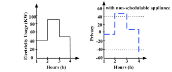
Figure 2: The household electricity usage and privacy within a non-schedulable appliance.

Comparing Fig. 1 and Fig. 2, one can see that the privacy breach occurs when a non-schedulable appliance operates in the scheduling horizon. Fig. 1 and Fig. 2 also demonstrates the trade-off between customers’ privacy and contentment requirements. In order to fit the privacy constrain, it is necessary to re-schedule the runtime of schedulable appliances and charging/discharging time of battery. Therefore, to ensure the customers’ privacy protection, understanding of the influence of non-schedulable appliance becomes essential.

III Runtime Appliance Scheduler

In this section, we present our approach to runtime cost-effective appliance scheduling to satisfy both privacy and contentment within considering the effect of non-schedulable appliance. Specifically, Section III-A describes the hierarchical structure of Runtime Appliance Scheduler, RAS. Section III-B introduces the specific scheduling problem to be be solved. Section III-C discusses the algorithm design for solving this problem.

III-A RAS Overview

The overall structure of RAS is shown in Fig. 3. The input components of the RAS is the schedule table and the current operation states of both schedulable and non-schedulable appliances as well as the battery state. Given these two input components, RAS can easily lookup the schedule table and find the optimal scheduling solution in real time. Among these input components, building the schedule table at the beginning of scheduling horizon plays the key role in RAS design.

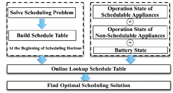
Figure 3: The overall structure of the runtime appliance scheduler.

III-B Scheduling Problem Formulation

The power management unit (PMU), utilizing models in Section II, is designed to schedule the battery and appliances operation. $x_{i}(t)$ ($i=\{1,2,\cdots,N\}$) for all schedulable appliances and $z(t)$ for the rechargeable battery. This optimization problem ($\sf{SP}$) can be expressed as

$$\scalebox{0.8}{\sf}{SP}:~{} {\sf{E}}\{\sum_{t=1}^{\tau}C(\mathbf{V}(t))\}={\sf{E}}\{\sum_{t=1}^{\tau}\left(c(t)l(t)\right)\}\;$$ min.

$$={\sf{E}}\{\sum_{t=1}^{\tau}c(t)\left(\mathbf{p}^{T}\min\left(\mathbf{V}(t),\mathbf{R}(t)\right)+w(t)\right)\}$$ (8a)

s.t. $$-\lambda\leq\left(\mathbf{p}^{T}\min\left(\mathbf{V}(t),\mathbf{R}(t)\right)+w(t)\right)-\overline{l}\leq\lambda,$$ (8b)

$$r_{i}(t+1)=\max\left(r_{i}(t)-\sum_{j=1}^{t}x_{i}(j),0\right),$$ (8c)

$$\sum_{t=1}^{\tau}{x_{i}(t)}=1,x_{i}(t)\in\{0,1\},\forall i\in\{1,2,\cdots,N\},$$ (8d)

$$B(t+1)=B(t)+z(t),0\leq B(t)\leq B_{\max}$$ (8e)

$$z_{\min}\leq z(t)\leq z_{\max}$$ (8f)

$$t=1,\cdots,\tau.$$

where $C(\mathbf{V}(t))=c(t)\left(\mathbf{p}^{T}\min\left(\mathbf{V}(t),\mathbf{R}(t)\right)+w(t)\right)$. $z_{\min}$ is the maximum discharged power, which is also the minimum charged power; $z_{\max}$ is the maximum charged power. $\sf{E}\{\cdot\}$ represents the expectation function. $\mathbf{V}(t)$ is the vector of decision variables for scheduling both the schedulable appliances and the rechargeable battery over the scheduling horizon. The expectation function is needed in the objective function above due to operation uncertainties of non-schedulable appliances.

Balancing electricity cost within a scheduling horizon in the presence of uncertainties of power consumption by non-schedulable appliances is thus a dynamic process. However, solving the optimization problem $(\sf{SP})$ at each time slot would be too time consuming. To address this issue, we present a hybrid approach.

III-C Scheduler Algorithm Design

In this subsection, we introduce a hybrid approach to solve the optimization problem $\sf{SP}$ in (8). In the problem $\sf{SP}$, the uncertainty effects introduced by non-schedulable appliances need to be carefully considered in the privacy constraint (8b), Because the immediately active operations by non-schedulable appliances lead to high peak load profiles and leak the appliance features. Lacking a comprehensive consideration of the influence of non-schedulable appliances can leak customers’ privacy. To handle this issue, we consider the worst influences of non-schedulable appliances’ operation in the customers’ privacy constraint (8b). We define a time zone of a peak load profile over the scheduling horizon as a worst privacy scenario. Mathematically, we define $\varphi=[t_{l},t_{u}]$ as a time zone for worst privacy scenario. $t_{l}$ and $t_{u}$ are a lower bound and a upper bound of time slot, separately. To guarantee the scheduler satisfies the privacy constraint (8b) even when the non-schedulable appliances operate in the worst scenario, we present a hybrid approach to handle it.

First, we assume that non-schedulable appliances are active at the worst privacy scenario. Once the non-schedulable appliances are assigned, we apply a dynamic programming like algorithm to solve the optimization problem $\sf{SP}$ and build a schedule table at the beginning of each scheduling horizon. This table contains $\tau$ columns where $\tau$ is the total number of time slots in the scheduling horizon, and a number of rows corresponding to the different states (described by the $r_{i}(t)$ and $B(t)$ values). Each entry in the table for time slot $t$ and state $s$ contains the assignment to $x_{i}(t)$ and $z(t)$ for a given set of $r_{i}(t)$ and $B(t)$ values. Note that we determine the assignment of $x_{i}(t)$ and $z(t)$ by consulting the table entry for time $t$ and state $s$ at the beginning of each time slot $t$. Second, we iteratively update worst privacy scenario after each schedule table building. Once the worst privacy scenario does not change anymore, we collect all these privacy scenarios as a potential set of operation time zone for non-schedulable appliances. And then, we re-apply a dynamic programming like algorithm to find the optimal assignment for schedulable appliances and rechargeable battery. This hybrid approach effectively takes into consideration of both non-schedulable and schedulable appliances.

III-C1 A Dynamic Programming Algorithm Design

Given the operation assignments of non-schedulable appliances at the worst privacy scenario, the schedule table can be obtained by solving optimization problem $\sf{SP}$. To ensure that the size of a schedule table is manageable, we assume that the remaining operation duration $r_{i}(t)$ ($\forall i$) and the battery state $B(t)$ are generally discretized to finite sets: $r_{i}(t)\in\mbox{$\bm{\mathcal{H}}$}=(\mathcal{H}_{i,1},\cdots,\mathcal{H}_{i,S_{i}})$ where $S_{i}=E_{i}/p_{i}$ ($\forall i$), and $B(t)\in\mbox{$\bm{\mathcal{B}}$}=(\mathcal{B}_{1},\cdots,\mathcal{B}_{M})$. Here $\bm{\mathcal{H}}$ is the $S$-element remaining operation duration set for the $i$-th schedulable appliance, and $\bm{\mathcal{B}}$ is the $M$-element battery state set. Let $\bm{\mathcal{G}}$ be the state set with $M\times\prod_{i=1}^{N}S_{i}$ elements including battery state set $\bm{\mathcal{B}}$ and remaining operation duration set $\bm{\mathcal{H}}$ ($\forall i$). Then, the structure of a schedule table can be shown as Table I. That is, a schedule table consists of $\tau$ sub-tables (corresponding to the columns in Table I), each of which is for a specific time slot $t$ from $1$ to $\tau$. Each sub-table consists of ${M\times\prod_{i=1}^{N}S_{i}}$ entries (corresponding to the state set), each of which contains the assignment to $\mathbf{x}(t)=[x_{1}(t),x_{2}(t),\cdots,x_{N}(t)]^{T}$.

The formulation (8) in Section III forms the basis for constructing the schedule table. Specifically, we adopt a backward recursive approach to solve problem $\sf{SP}$. Given the initial state $\mathcal{G}_{1}$ at time slot $1$, ($\mathcal{G}_{1}\in\mbox{$\bm{\mathcal{G}}$}$), we denote $\mathcal{F}_{1}(\mathcal{G}_{1})$ as the optimal value of (8), which can be obtained recursively due to the principle of optimality [5]. Because the value of $C(\mathbf{V}(t))$ can be precisely determined since the operation states of both schedulable and non-schedulable appliances as well as the battery states prior to $t$ are known. Only the future states are not known. Thus we can rewrite (8) as

$$\scalebox{0.8}{\sf}{SP}: \mathcal{F}_{1}(\mathcal{G}_{1})=\min\left\{C(\mathbf{V}(1))+\sf{E}_{\mbox{$\bm{\mathcal{G}}$}}\left\{\sum_{t=2}^{\tau}C(\mathbf{V}(t))\right\}\right\}$$ (9a)

s.t. $$-\lambda\leq\left(\mathbf{p}^{T}\min\left(\mathbf{V}(t),\mathbf{R}(t)\right)+w(t)\right)-\overline{l}\leq\lambda,$$ (9b)

$$r_{i}(t+1)=\lceil\max(r_{i}(t)-\sum_{j=1}^{t}x_{i}(j),0)\rceil$$

$$r_{i}(t),r_{i}(t+1)\in\mbox{$\bm{\mathcal{H}}$}$$ (9c)

$$B(t+1)=B(t)+z(t),$$

$$B(t),B(t+1)\in\mbox{$\bm{\mathcal{B}}$},$$ (9d)

$$\sum_{t=1}^{\tau}{x_{i}(t)}=1,x_{i}(t)\in\{0,1\},$$ (9e)

$$z_{\min}\leq z(t)\leq z_{\max}$$ (9f)

$$t=\tau-1,\tau-2,\cdots,1,\hskip 10.00002pti=1,2,\cdots,N\vspace*{-3ex}$$

where $\mathbf{V}(1)$ corresponds to those $x_{i}(1)$ and $z(1)$ that result in state $\mathcal{G}_{1}$ at time $t=1$. $\sf{E}_{\mbox{$\bm{\mathcal{G}}$}}$ describes the expectation operation over the all possible states $\bm{\mathcal{G}}$. Furthermore, (9c) denotes the state transition of remaining operation duration for all schedulable appliances, which is constrained in the finite set $\bm{\mathcal{H}}$. The (9d) denotes the battery state transition that is also constrained in the finite set $\bm{\mathcal{B}}$.

In a nutshell, the optimal values for arbitrary time slots $(t)$ to $1$ are determined in a backward recursive manner by considering state transitions from all possible state $\mathcal{G}_{t+1}$ at $t+1$ to $\mathcal{G}_{t}$ at $t$ ($\mathcal{G}_{t},~{}\mathcal{G}_{t+1}\in\mbox{$\bm{\mathcal{G}}$}$) and the constraints in (9), which is shown as follows.

$$\scalebox{0.8}{}{\mathcal{F}_{t}(\mathcal{G}_{t})=\min\{C(\mathbf{V}(t))+\sf{E}_{\mbox{$\bm{\mathcal{G}}$}}\{\mathcal{F}_{t+1}(\mathcal{G}_{t+1})\},}$$ (10)

where $C(\mathbf{V}(t))$ is the electricity cost value in state $\mathcal{G}_{t}$ at time slot $t$, which corresponds to those $x_{i}(t)$ and $z(t)$. $\mathcal{G}_{t}$ and $\mathcal{G}_{t+1}$ are the state at time slot $t$ and $t+1$, respectively. $\sf{E}_{\mbox{$\bm{\mathcal{G}}$}}\{\mathcal{F}_{t+1}(\mathcal{G}_{t+1})\}$ is the expected sum of the minimal cost value over all possible states $\bm{\mathcal{G}}$ for time slots $t+1,t+2,\cdots,\tau$. Note that, the backward recursive approach firstly calculates the optimal value $\mathcal{F}_{\tau}(\mathcal{G}_{\tau})$ for time slot $\tau$ with the known state $\mathcal{G}_{\tau}$, which is shown as follow.

$$\scalebox{0.8}{}{\mathcal{F}_{\tau}(\mathcal{G}_{\tau})=\min C(\mathbf{V(\tau)}).}$$ (11)

These processes are summarized in Algorithm 1.

TABLE I: Structure of the schedule table.

State ($B(t),r_{1}(t),r_{2}(t),\cdots,r_{N}(t)$)	Time Slot
	1	2	$\cdots$	$\tau$
$\mathcal{B}_{1},\mathcal{H}_{1,1},\mathcal{H}_{2,1},\cdots,\mathcal{H}_{N,1}$	$\mathbf{x}(1)$	$\mathbf{x}(2)$	$\cdots$	$\mathbf{x}(\tau)$
$\mathcal{B}_{2},\mathcal{H}_{1,1},\mathcal{H}_{2,1},\cdots,\mathcal{H}_{N,1}$	$\mathbf{x}(1)$	$\cdots$	$\mathbf{x}(t)$
$\cdots$	$\cdots$	$\cdots$	$\cdots$	$\cdots$
$\mathcal{B}_{M},\mathcal{H}_{1,S_{1}},\mathcal{H}_{2,S_{2}},\cdots,\mathcal{H}_{N,S_{N}}$	$\mathbf{x}(1)$	$\mathbf{x}(2)$	$\cdots$	$\mathbf{x}(\tau)$

1:  Initialization

2:   Given initial state $\mathcal{G}_{1}$, $M$-element battery state set $\bm{\mathcal{B}}$, $S$-element remaining operation duration set $\bm{\mathcal{H}}$ for $i$-th schedulable appliance ($\forall i$), number of time slots $\tau$, and the assignment active operations of non-schedulable appliances

3:  Recursive calculation

4:   for $t=\tau$ to $1$

5:    for $\mathcal{G}_{t}=\mathcal{G}_{1}$ to $\mathcal{G}_{M\times\prod_{i=1}^{N}S_{i}}$

6:     if $t=\tau$, Calculate $\mathcal{F}_{\tau}(\mathcal{G}_{\tau})$ by (11);

7:     else, Calculate $\mathcal{F}_{t}(\mathcal{G}_{t})$ by solving (10) until $\mathcal{F}_{1}(\mathcal{G}_{1})$ is obtained.

8:  Return Optimal value $\mathcal{F}_{1}(\mathcal{G}_{1})$, and its corresponding $x_{i}(t)$ ($\forall i$) and $z(t)$ for each time slot $t$ ($\forall t\in\tau$).

Algorithm 1 : A Dynamic Programming Algorithm Design

III-C2 Privacy-Aware Scheduler Design

In the description of Algorithm 1, the assignment of active operations of non-schedulable appliances are known before the dynamic process. Considering multiple worst privacy scenarios, we iteratively assign non-schedulable appliances into worst scenario and generate it as a new privacy constraint, and then use assignment active operations of non-schedulable appliances. Finally, the problem $\sf{SP}$ in (9) is solved. To simplify the problem, we assume that the power consumption of any non-schedulable appliance within each time slot during the appliance’s active operation is a constant value, defined as $p_{j}$ ($\forall j=1,2,\cdots,W$). $W$ is the total number of non-schedulable appliances. Associated with the set of time zone for worst privacy scenarios ($\Omega$), we define a binary variable $h_{j}(t,\varphi)$. If $h_{j}(t,\varphi)=1$, the $j$-th non-schedulable appliance actives its operation at time slot $t$ in worst privacy scenario $\varphi$. Otherwise $h_{j}(t,\varphi)=0$. The definition of $h_{j}(t,\varphi)$ is shown as follows.

$$\scalebox{0.8}{}\begin{aligned} h_{j}(t,\varphi)&=\begin{cases}1&\text{if }t\in\varphi~{}(\varphi\in\Omega),\\ 0&\text{else }\text{Otherwise},\end{cases}\end{aligned}\forall j=1,2,\cdots,M.$$ (12)

Thus, we re-write the load model for non-schedulable appliances. The total power consumptions of all non-schedulable appliances at time slot $t$ is expressed as

$$\scalebox{0.8}{}{w(t,\varphi)=\sum_{j=1}^{W}h_{j}(t,\varphi)p_{j}.}\vspace*{-5ex}$$ (13)

According to (II-A3) and (13), the updated privacy model can be re-written as

$$\scalebox{0.8}{}{-\lambda\leq g\left(\mathbf{V}(t),\varphi\right)\leq\lambda,~{}\forall\varphi\in\Omega,}\vspace*{-5ex}$$ (14)

where $g\left(\mathbf{V}(t),\varphi\right)=\mathbf{p}^{T}\min\left(\mathbf{V}(t),\mathbf{R}(t)\right)+w(t,\varphi)-\overline{l}$. Taking account of the set of worst privacy scenarios ($\Omega$) and updated privacy constraint (14), the scheduling problem $(\sf{SP}(\Omega))$ is expressed as

$$\sf{SP}(\Omega): \mathcal{F}_{1}(\mathcal{G}_{1})=\min\left\{C(\mathbf{V}(1))+\sf{E}_{\mbox{$\bm{\mathcal{G}}$}}\left\{\sum_{t=2}^{\tau}C(\mathbf{V}(t))\right\}\right\}$$ (15a)

s.t. $$-\lambda\leq g\left(\mathbf{V}(t),\varphi\right)\leq\lambda,~{}\forall\varphi\in\Omega$$ (15b)

$$r_{i}(t+1)=\max\left(r_{i}(t)-\sum_{j=1}^{t}x_{i}(j),0\right),$$ (15c)

$$\sum_{t=1}^{\tau}{x_{i}(t)}=1,x_{i}(t)\in\{0,1\},\forall i\in\{1,2,\cdots,N\},$$ (15d)

$$B(t+1)=B(t)+z(t),0\leq B(t)\leq B_{\max}$$ (15e)

$$z_{\min}\leq z(t)\leq z_{\max}$$ (15f)

$$t=1,\cdots,\tau.$$

In the optimization problem $\sf{SP}(\Omega)$,  (15b) includes the set of worst privacy scenarios $\Omega$, which consists of infinite constraints. Inspired by semi-infinite programming technique, we introduce a hybrid approach to solve the problem $\sf{SP}(\Omega)$, which is summarized in Algorithm 2. In Algorithm 2, we denote $\mathbf{V}^{*}_{k}$ and $\mathbf{V}^{*}_{k-1}$ as the feasible solutions of problem $\sf{SP}(\Omega_{k})$ and $\sf{SP}(\Omega_{k-1})$, respectively. Note That at the $k$-th iteration of the Algorithm 2, we update the privacy constraint (15b) using $\Omega_{k}=\Omega_{k-1}\cup\{\varphi_{k}\}$. And then we solve a subproblem $\sf{SP}(\Omega_{k})$ with $\varphi_{k}$ satisfying worst privacy scenario requirement. Meanwhile, the Algorithm 2 converges after several iterations and produces an approximate optimal solution for $\sf{SP}(\Omega)$ if the worst privacy scenario doesn’t change anymore.

Convergence analysis: Let $\mathcal{V}$ denote the feasible region of problem $\sf{SP}$. At the $k$-th iteration, when constraints (15c), (15d), (15e) and (15f) are satisfied, the feasible region of problem $\sf{SP}(\Omega_{k})$ with worst privacy scenarios $\Omega_{k}$ is expressed as follows.

$$\scalebox{0.8}{}{\mathcal{V}_{k}:=\{\mathbf{V}|-\lambda\leq g\left(\mathbf{V},\varphi\right)\leq\lambda,~{}\forall\varphi\in\Omega_{k}\}}$$ (16)

To prove Algorithm 2 converge to an optimal solution when $k\rightarrow\infty$, the following two lemmas are needed.

Lemma 1.

For each $k\geq 1$, if Algorithm 2 does not stop at this iteration, $\mathcal{V}_{k}\subseteq\mathcal{V}_{k-1}$ holds, where $\mathcal{V}_{k-1}$ and $\mathcal{V}_{k}$ are the feasible regions of optimization problem $\sf{SP}(\Omega_{k-1})$ and $\sf{SP}(\Omega_{k})$, respectively.

Proof.

By contradiction, suppose this Lemma is false: for each $k\geq 1$, if Algorithm 2 does not stop at this iteration, the $\mathcal{V}_{k}\nsubseteq\mathcal{V}_{k-1}$. This means that a feasible region $\mathcal{V}_{k-1}$ is a subset of $\mathcal{V}_{k}$. Therefore, $\mathcal{V}_{k-1}$ is also the feasible regions of problem $\sf{SP}(\Omega_{k})$, which satisfies privacy constraint (15b). Based on the definition of feasible region, the following equation (17) holds.

$$\scalebox{0.8}{}{\mathcal{V}_{k-1}:=\{\mathbf{V}|-\lambda\leq g\left(\mathbf{V},\varphi\right)\leq\lambda,~{}\forall\varphi\in\Omega_{k}\}}$$ (17)

Meanwhile, $\mathcal{V}_{k-1}$ is also the feasible regions of problem $\sf{SP}(\Omega_{k-1})$. Therefore, $\mathcal{V}_{k}\nsubseteq\mathcal{V}_{k-1}$ yields $\Omega_{k}=\Omega_{k-1}$. However, $\Omega_{k}:=\Omega_{k-1}\cup\{\varphi_{k}\}$ holds and $\varphi_{k}$ exists, because Algorithm 2 does not stop at $k$-th iteration, contradicting our assumption. Thus, this lemma holds.

Lemma 2.

For $k\geq 1$, if $k\rightarrow\infty$, the subproblem $\sf{SP}(\Omega_{k})$ has an optimal solution.

Proof.

When $k\rightarrow\infty$, the set of worst privacy scenarios $\Omega_{k}\rightarrow\Phi$, where $\Phi$ is the set of all possible worst privacy scenarios. Once $\Omega_{k}$ reaches $\Phi$, the feasible region $\mathcal{V}_{k}$ of $\sf{SP}(\Omega_{k})$ becomes a unique and smallest feasible region due to lemma 1. Thus, the subproblem $\sf{SP}(\Omega_{k})$ has an optimal solution.

1:  Initialization

2:   Apply the Algorithm 1 to solve the problem $\sf{SP}$ without considering non-schedulable appliances

3:   Find the worst privacy scenario $\varphi_{0}$. Set $\Omega_{0}:=\{\varphi_{0}\}$

4:  Iterative programming calculation

5:   Apply the Algorithm 1 to solve $\sf{SP}(\Omega_{0})$ and obtain an optimal scheduling variable $\mathbf{V}^{*}_{0}$

6:   Set $k:=1$

7:   Find the worst privacy scenario $\varphi_{k}$

8:    if $\varphi_{k}=\varphi_{k-1}$, then STOP, return optimal scheduling variable $\mathbf{V}^{*}_{k}$

9:    else, let $\Omega_{k}:=\Omega_{k-1}\cup\{\varphi_{k}\}$

10:   Apply the Algorithm 1 to solve problem $\sf{SP}(\Omega_{k})$ to obtain an optimal scheduling variable $\mathbf{V}^{*}_{k}$

11:   Set $k:=k+1$ and got to Step 7

Algorithm 2 : Iterative Alternative Algorithm

IV Numerical Simulations

This section evaluates the proposed runtime scheduling framework using real-world household data. The proposed iterative alternative algorithm conducts the worst scenario optimization to effectively generate cost-efficient scheduling solution with privacy protection guarantee. Section IV-A demonstrates scheduling results based on real world power consumption. Section IV-B campares the evaluation results of the system without a non-schedulable appliance to the system with a non-schedulable appliance. Section IV-C demonstrates the impacts of battery capacity on the scheduler behavior.

IV-A Real world benchmark

We first summarize the simulation-based experimental settings.

Appliance data sets and types: We have selected five household appliances data from a ECO data set [2]. This ECO data set includes aggregate and plug-in appliances’ power consumptions of households in Switzerland over a period of 8 months. These data were collected customer daily usage with $86,400$ measurements per day. Two types of appliances are considered: schedulable appliances (i.e., clothes dryer, washing machine, dishwasher, stove, and refrigerator) and non-schedulable appliances (i.e., PC, stereo, TV, and laptop). To demonstrate the proposed approach, we consider a household having three schedulable appliances and two non-schedulable appliances. We set the entire work load and power consumptions of three schedulable appliances ($1$, $2$, and $3$) as follows: ($E_{1}=70.7W$, $p_{1}=35.38Wh$), ($E_{2}=313.2W$, $p_{2}=156.59Wh$), and ($E_{3}=230.2W$, $p_{3}=76.73Wh$). For the two non-schedulable appliances ($4$ and $5$), the entire work load $E_{4}=106.97W$ and $E_{5}=33.73W$. Based on the ECO data set [2], the appliance $4$ and $5$ usually operates at time slot $t=[7,12]$ and $t=[1,6]$ with a high possibility, respectively. The remaining operation duration set $\bm{\mathcal{H}}$ is discretized as

$$\scalebox{0.8}{}{\mbox{$\bm{\mathcal{H}}$}=\{0,1,\cdots,\lceil E_{i}/p_{i}\rceil\}.}$$

The electricity price is adopted by the public released data from Ameren Corporation [1].

Rechargeable battery parameters: The maximum battery capacity $B_{max}=750$ Wh and the initial state of battery ($B(1)$) is 0. To apply the proposed iterative alternative algorithm, we discretized the state set $\bm{\mathcal{B}}$ of battery as

$$\scalebox{0.8}{}{\mbox{$\bm{\mathcal{B}}$}=\{0,1,2,\cdots,B_{max}\}.}$$

The battery charged/discharged power set $\mathcal{Z}=\{z|50Wh\leq z\leq 250Wh\}$. To speed up the table building process, a local version of the algorithm was used in experiment where $z$ was not discretized. In terms of privacy concerns, we set $\lambda=80$.

Scheduling horizon: The length of the scheduling time slot is one hour. The overall scheduling horizon is set to be 12 hours. The simulation result is shown in Fig. 4. It can be observed that the original power consumption curve exceeded the pravicy constrain and the shape peak is sensitive to be detected by attacker. The scheduled power consumption curve followed the privacy constrain between the upper boundary and lower boundary and the curve is relative smooth.

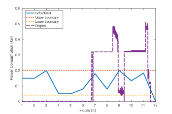
Figure 4: Real world scheduling result.

TABLE II: Evaluation environment setting

Battery total capacity	0.2 kW
Battery charging/discharging rate	0 kW to 0.1 kW
Non-schedulable appliances Runtime	1 (hours)

IV-B Scheduler Evaluation

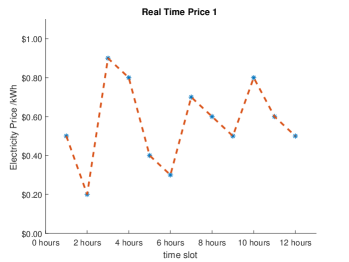
Figure 5: The real time price for performance evaluation.

TABLE III: Schedulable module evaluation results

Time Slot	1	2	3	4	5	6	7	8	9	10	11	12
App 1	0	0	0	0	0	1	1	1	1	1	0	0
App 2	0	0	0	1	1	1	0	0	0	0	0	0
App 3	1	1	0	0	0	0	0	0	0	0	0	0

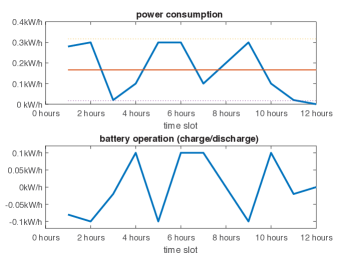
Figure 6: Scheduling results for schedulable module.

TABLE IV: Non-schedulable module evaluation results

Time Slot	1	2	3	4	5	6	7	8	9	10	11	12
App 1	0	0	0	0	1	1	1	1	1	0	0	0
App 2	0	0	0	0	0	0	0	0	1	1	1	0
App 3	0	1	1	0	0	0	0	0	0	0	0	0

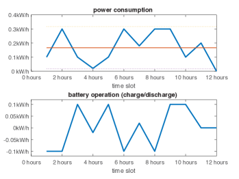
Figure 7: Scheduling results for non-schedulable module.

Section IV-B will evaluate the system using the setting as shown in Table II. Considering the real-world scenario, the charging/discharging rate of a battery varies in the scheduling horizon. Given the unknown starting time of non-schedulable appliance, the scheduler system defines a certain range of time as the potential starting time of non-schedulable appliance based on its historical usage pattern. In this test, there are three assumptions made. First, each appliance is allowed to run only once and it will stop when its runtime finished. Second, the power consumption of any schedulable appliances within each time slot during the appliances active is a constant value. Third, all appliances have to be finished before the end.

Fig. 5 illustrates the real-time electricity price over 12 hours scheduling horizon. Given the real-time electricity price, online scheduler decides on the actual appliance usage pattern. Table III and Fig. 6 demonstrate the proposed operation of schedulable module and the operation of battery and real time power consumption, respectively. It can be noticed that the power consumption followed the privacy constraint which successfully protect the behavior of all appliance. In the battery operation, the battery will gain energy at the positive value and release energy at negative value in the battery operation as shown in Fig. 6. The non-schedulable module evaluation results are shown in Table IV and Fig. 7, respectively. In the Table III and Table IV, for each appliance, the digits ’1’ represent that the appliance is switched on and the digits ’0’ represent that the appliance is switched off. In this scheduling results, the non-schedulable appliance did not run. But the system prepared for it between the first six hours which define as the non-schedulable time zone in this instance. The battery will reserve enough energy for the unpredictable appliance, thus it will follow the privacy constrain. In this module, the system will prepare for the worst case of privacy risk and also find the lowest electricity billing price solution.

IV-C Sensitivity analysis of battery capacity and billing price

In this section, we analyze the effect of electricity price and battery capacity on the scheduler the system. The experiment setup of system remains the same as discussed in the Section IV-B. Fig. 8, marked as the second price, is modified from Fig. 5. The minimum electricity price was switched out from the non-schedulable time zone in Fig. 8. To evaluate the effect of price, the test will be repeated with the second price.

The evaluation results is shown in Fig. 9. The X coordinate represents the battery size and Y coordinate represents the amount of billing price in the U.S. Dollar. As increasing the battery capacity, the billing price converges to a constant value and it indicted the battery capacitor is sufficient in this certain scenario. As shown in Fig. 9, the system is very sensitive when the battery capacity is relative small. Because the battery is not sufficient to reserve enough energy in a lower price time slot, the billing price drop rapidly when the capacity increase from 8 kW to 20 kW. For the non-schedulable module, it can be noticed that the battery must reserve electricity for the non-schedulable appliance, thus the the total price is slightly higher than the price for a schedulable module. In the second price instance, the minimum price is out of non-schedulable active time range and the system will schedule the battery to reserve energy to prepare for the non-schedulable appliance at higher price time slot. Hence, the total price will increase since the scheduler has to follow the privacy constrain. Therefore, the price drops more when the battery capacity increases in non-schedulable module.

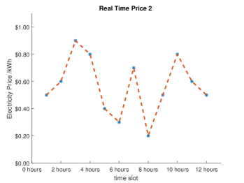
Figure 8: Modified real time price for sensitivity analysis.

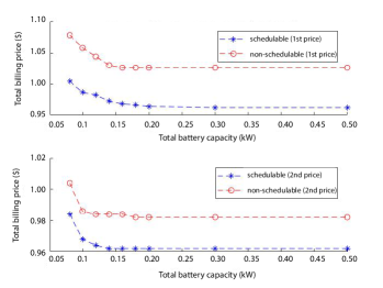
Figure 9: Total billing price VS total battery capacity sizes.

The scheduler is able to protect the appliance behavior information and also able to obtain a better price solution. The scheduler is build with high flexibility and it can handle more complex scenarios, such as flexible battery charging/discharging rate, a smart home system with a large number of schedulable appliances and non-schedulable appliances.

V Summary and Future Work

Smart homes promise many potentials but also raise new privacy concerns. This paper considers the effects of fake guideline electricity price and non-schedulable appliances’ operation uncertainties in appliance scheduling for smart homes. Different from existing research, this work aims to not only minimize electricity cost but also protect customers’ privacy. The proposed framework, PACES, is evaluated using publicly released households’ data sets. Our experimental study shows that PACES can effectively protect customers’ privacy and satisfy their immediate service requirement with a small increase in electricity cost. PACES can be somewhat time consuming if a household has a large number of appliances. There are great research opportunities in the area of privacy protection and cost reduction for smart homes.

References

- [1] Ameren day-ahead prices. https://www2.ameren.com/RetailEnergy/RealTimePrices.
- [2] Electricity consumption and occupancy. http://data-archive.ethz.ch/delivery/DeliveryManagerServlet?dps_pid=IE594964.
- [3] K. Al-Jabery, D. C. Wunsch, J. Xiong, and Y. Shi. A novel grid load management technique using electric water heaters and q-learning. In 2014 IEEE International Conference on Smart Grid Communications (SmartGridComm), pages 776–781. IEEE, 2014.
- [4] K. Al-Jabery, Z. Xu, W. Yu, D. C. Wunsch, J. Xiong, and Y. Shi. Demand-side management of domestic electric water heaters using approximate dynamic programming. IEEE Transactions on Computer-Aided Design of Integrated Circuits and Systems, 36(5):775–788, 2017.
- [5] D. P. Bertsekas, D. P. Bertsekas, D. P. Bertsekas, and D. P. Bertsekas. Dynamic programming and optimal control, volume 1. Athena Scientific Belmont, MA, 1995.
- [6] Z. Chen and L. Wu. Residential appliance dr energy management with electric privacy protection by online stochastic optimization. IEEE Transactions on Smart Grid, 4(4):1861–1869, 2013.
- [7] G. Kalogridis, C. Efthymiou, S. Z. Denic, T. A. Lewis, and R. Cepeda. Privacy for smart meters: Towards undetectable appliance load signatures. In IEEE International Conference on Smart Grid Communications, pages 232–237, 2010.
- [8] E. Liu, P. You, and P. Cheng. Optimal privacy-preserving load scheduling in smart grid. In 2016 IEEE Power and Energy Society General Meeting (PESGM), pages 1–5, 2016.
- [9] Y. Liu, S. Hu, J. Wu, Y. Shi, Y. Jin, Y. Hu, and X. Li. Impact assessment of net metering on smart home cyberattack detection. In Proceedings of the 52nd Annual Design Automation Conference, page 97. ACM, 2015.
- [10] Y. Liu, S. Hu, J. Wu, Y. Shi, Y. Jin, Y. Hu, and X. Li. Smart home cybersecurity considering the integration of renewable energy. In Smart Cities and Homes, pages 173–189. Elsevier, 2016.
- [11] S. McLaughlin, P. McDaniel, and W. Aiello. Protecting consumer privacy from electric load monitoring. In Proceedings of the 18th ACM conference on Computer and communications security, pages 87–98. ACM, 2011.
- [12] A. Molina-Markham, P. Shenoy, K. Fu, E. Cecchet, and D. Irwin. Private memoirs of a smart meter. In ACM workshop on embedded sensing systems for energy-efficiency in building, pages 61–66, 2010.
- [13] P. Palensky and D. Dietrich. Demand side management: Demand response, intelligent energy systems, and smart loads. IEEE transactions on industrial informatics, 7(3):381–388, 2011.
- [14] L. Sankar, S. R. Rajagopalan, and S. Mohajer. Smart meter privacy: A theoretical framework. IEEE Transactions on Smart Grid, 4(2):837–846, 2013.
- [15] O. Tan, D. Gunduz, and H. V. Poor. Increasing smart meter privacy through energy harvesting and storage devices. IEEE Journal on Selected Areas in Communications, 31(7):1331–1341, 2013.
- [16] J. Wu, J. Liu, X. S. Hu, and Y. Shi. Privacy protection via appliance scheduling in smart homes. In 2016 IEEE/ACM International Conference on Computer-Aided Design (ICCAD), pages 1–6, 2016.
- [17] J. Wu, J. Xiong, and Y. Shi. Efficient location identification of multiple line outages with limited pmus in smart grids. IEEE Transactions on Power Systems, 30(4):1659–1668, 2015.
- [18] X. Xu, Y. Ding, S. X. Hu, M. Niemier, J. Cong, Y. Hu, and Y. Shi. Scaling for edge inference of deep neural networks. Nature Electronics, 1(4):216, 2018.
- [19] X. Xu, F. Lin, A. Wang, X. Yao, Q. Lu, W. Xu, Y. Shi, and Y. Hu. Accelerating dynamic time warping with memristor-based customized fabrics. IEEE Transactions on Computer-Aided Design of Integrated Circuits and Systems, 37(4):729–741, 2018.
- [20] X. Xu, F. Lin, W. Xu, X. Yao, Y. Shi, D. Zeng, and Y. Hu. Mda: A reconfigurable memristor-based distance accelerator for time series mining on data centers. IEEE Transactions on Computer-Aided Design of Integrated Circuits and Systems, 2018.
- [21] X. Xu, Q. Lu, L. Yang, S. Hu, D. Chen, Y. Hu, and Y. Shi. Quantization of fully convolutional networks for accurate biomedical image segmentation. In Proceedings of the IEEE Conference on Computer Vision and Pattern Recognition, pages 8300–8308, 2018.
- [22] X. Xu, D. Zeng, W. Xu, Y. Shi, and Y. Hu. An efficient memristor-based distance accelerator for time series data mining on data centers. In 2017 54th ACM/EDAC/IEEE Design Automation Conference (DAC), pages 1–6. IEEE, 2017.
- [23] L. Yang, X. Chen, J. Zhang, and H. V. Poor. Cost-effective and privacy-preserving energy management for smart meters. IEEE Transactions on Smart Grid, 6(1):486–495, 2015.
- [24] Y. Yuan, Z. Li, and K. Ren. Modeling load redistribution attacks in power systems. IEEE Transactions on Smart Grid, 2(2):382–390, 2011.
- [25] S. Yue, J. Chen, Y. Gu, C. Wu, and Y. Shi. Dual-pricing policy for controller-side strategies in demand side management. In IEEE International Conference on Smart Grid Communications, pages 357–362, 2011.