Cosmological Parameters from the BOSS Galaxy Power Spectrum
Abstract
We present cosmological parameter measurements from the publicly available Baryon Oscillation Spectroscopic Survey (BOSS) data on anisotropic galaxy clustering in Fourier space. Compared to previous studies, our analysis has two main novel features. First, we use a complete perturbation theory model that properly takes into account the non-linear effects of dark matter clustering, short-scale physics, galaxy bias, redshift-space distortions, and large-scale bulk flows. Second, we employ a Markov-Chain Monte-Carlo technique and consistently reevaluate the full power spectrum likelihood as we scan over different cosmologies. Our baseline analysis assumes minimal CDM, varies the neutrino masses within a reasonably tight range, fixes the primordial power spectrum tilt, and uses the big bang nucleosynthesis prior on the physical baryon density . In this setup, we find the following late-Universe parameters: Hubble constant km s-1Mpc-1, matter density fraction , and the mass fluctuation amplitude . These parameters were measured directly from the BOSS data and independently of the Planck cosmic microwave background observations. Scanning over the power spectrum tilt or relaxing the other priors do not significantly alter our main conclusions. Finally, we discuss the information content of the BOSS power spectrum and show that it is dominated by the location of the baryon acoustic oscillations and the power spectrum shape. We argue that the contribution of the Alcock-Paczynski effect is marginal in CDM, but becomes important for non-minimal cosmological models.
INR-TH-2019-016
CERN-TH-2019-132
1 Introduction
Density fluctuations traced by galaxies are an important source of information about our Universe. They can be used to probe perturbations on scales similar to those measured in the cosmic microwave background (CMB) observations, but at a very different epoch of cosmic evolution and in a very different physical environment. Future galaxy surveys with their increasingly larger volumes have a great potential to provide the most stringent tests of CDM and possibly lead to new discoveries [1, 2, 3, 4].
The increasing precision of the large-scale structure (LSS) surveys calls for a consistent and accurate theoretical modeling which is easy to implement in the data analysis pipeline. In this paper we focus on some aspects of this problem. In particular, we use a rigorous perturbation theory model for the redshift-space galaxy power spectrum (PS) to measure cosmological parameters from the publicly-available444We use the data that can be accessed via https://fbeutler.github.io/hub/hub.html, see also http://www.sdss3.org/science/boss_publications.php . Baryon Oscillation Spectroscopic Survey (BOSS) Data Release 12 (DR12) published in 2016.555We use directly the power spectrum multipoles provided by the BOSS collaboration. The details of the data are given in Sec. 3. Similar full-shape (FS) analyses of the power spectrum multipole moments [5, 6] or position-space correlation function and redshift-space wedges [7, 8, 9] have been already done in the past. Our motivation to repeat this exercise is twofold.
First, despite significant progress in understanding the nonlinear evolution of large-scale structure and biased tracers, many recently developed theoretical tools are not routinely used in the data analysis. These new results can be roughly split into two categories. The first category comprises consistent perturbative descriptions developed to improve matter clustering modeling in the mildly nonlinear regime. This includes nonlinearities in the dark matter fluid [10, 11], the bias model [12, 13, 14, 15] (for a review see [16]), and redshift space distortions [17, 18]. In all these cases one can systematically, order by order in perturbation theory, write down all independent contributions to the nonlinear density field. These contributions are derived using equations of motion and general symmetry arguments, such as mass and momentum conservation, and the equivalence principle. The functional form of these contributions is entirely fixed by these arguments, but the amplitudes are unknown. These contributions are related to the familiar bias parameters and less popular “counterterms,” whose purpose is to capture the impact of unknown small-scale physics on the long-wavelength fluctuations. Any consistent theoretical model has to keep all these parameters in the fit in order to obtain unbiased estimates of cosmological parameters.
The second category of analytical results is related to the accurate description of the baryon acoustic oscillations (BAO). It has long been known that the shape of the BAO peak is very sensitive to large displacements or bulk flows [19, 20, 21]. Their effect on the density field can be significant since the typical displacements of galaxies are of order Mpc. However, the basic formulation of Eulerian Perturbation Theory [22] treats bulk flows only perturbatively.666In Lagrangian Perturbation Theory (LPT) this is not the case since the bulk flows correspond to the linear displacement and they are resummed by construction. This is the reason why even in the Zel’dovich approximation the shape of the BAO peak is described rather well. For some more recent progress in modeling the BAO peak for dark matter and biased tracers in real and redshift space using models based on LPT see [23, 24]. One practical disadvantage of LPT-based models is that evaluation of power spectra is numerically rather demanding. This problem has recently been resolved in a number of works within different but equivalent perturbation theory schemes and in various approximations [25, 26, 27, 28, 29, 30, 31]. In a nutshell, large bulk flows are induced by the long-wavelength or “infrared” modes, whose dominant physical effect is a simple translation of matter. This allows for an exact treatment beyond perturbation theory, which was called infrared (IR) resummation [25]. Using IR-resummation the shape of the BAO wiggles can be predicted to very high precision (including higher order loops if necessary). Crucially, this procedure requires no fitting parameters. This is very different from usual, more phenomenological methods to predict the spread of the BAO peak and this difference is relevant even for the analysis of data from current surveys. We implement all these novel results in our theoretical model for the power spectrum.
Let us stress that the theoretical description of non-linear BAO damping may not be the most optimal way to extract cosmological information. Rather than modeling the damping of the BAO peak, one can undo this damping by means of BAO reconstruction at the catalog level [32, 33]. This procedure effectively transfers information from higher order -point functions to the 2-point function. The standard BAO reconstruction does sharpen the BAO wiggles, but it also introduces some distortions in the broadband part, which are hard to model analytically. Even though some progress towards a consistent reconstruction of the full initial density field has recently been made [34, 35, 36], the available methods have not been extensively tested for biased tracers in redshift space and we leave exploration of this direction for future work.
Our second motivation to reanalyze the BOSS data is to perform a consistent Markov-Chain-Monte-Carlo (MCMC) study that samples all relevant cosmological and nuisance parameters without assuming the CMB priors. This is not a standard practice in the FS studies, in part due to a relatively high computational cost of a direct numerical evaluation of perturbation theory loop integrals. Some exceptions are BOSS analyses of the position-space correlation function and redshift-space wedges [7, 8, 9] where all relevant parameters in the MCMC chains were varied, but only in combination with the Planck CMB likelihood. A more conventional approach to FS analysis is to compute the power spectrum shape for one fiducial cosmology and parametrize deviations from it by means of the following scaling parameters:
| (1.1) |
where is the effective redshift of the data, is the sound horizon at the drag epoch (which sets the BAO frequency), is the Hubble parameter and the angular diameter distance, is the logarithmic growth rate (, where is the linear growth factor and is the scale factor), is the late-time rms mass fluctuation in the spheres of comoving radius . The parametrization above is motivated by the BAO studies, in which and are the most relevant parameters. However, the use of these scaling parameters is not entirely correct in the case of the full-shape analysis. To see this, let us consider a variation of the physical dark matter density with all other parameter fixed. This variation will have an impact not only on , but also on the amount of the short-scale baryon suppression and the position of the PS peak. This argument suggests that if the PS shape is fixed, must be fixed as well for consistency. In this case the parameterization (1.1) becomes a correct description of the Alcock-Paczynski effect [37], which does not assume any priors on the radial and angular distances.
A rational behind the scaling parameter analysis is that ultimately one intends to combine LSS and CMB data to constrain a class of non-minimal cosmological models that are described by the standard physics at early times but modify the late-time expansion, e.g. dynamical dark energy. The CMB data provide us with (sub-)percent priors on the physical densities of baryons and dark matter, which nearly fix the PS shape in the combined analysis. In that case the PS complements the CMB with the geometric and distance information that is indeed captured by the -parameters in Eq. (1.1). The standard analysis thus assumes strong priors on the early physics, i.e. the physical densities of baryons and dark matter, which are the most relevant parameters defining the power spectrum shape. These priors will be referred to as “shape priors” in what follows.
In practice, one may face situations that require a more general treatment. These cases include the use of different priors, the study of degeneracies between cosmological and nuisance parameters, the information content of the power spectrum shape, and exploring various extensions of the minimal CDM that include physics, which is not captured by a simple change of the late-time expansion and scale-independent growth factor. These include, e.g. massive neutrinos or models with non-standard early physics. In all these cases the common approach becomes inadequate. Besides, the future LSS data may supersede Planck, which also calls for a reassessment of the standard analysis pipeline.
In the most general setup it would be ideal to measure cosmological parameters directly from the shape of the observed multipoles, independently of the chosen priors. In that case one would have to model the whole evolution of perturbations for a given cosmological model in the same way as it is usually done in the CMB data analysis. In this paper we analyze the BOSS data in this general way. This task requires a numerical routine able to generate theoretical templates for the non-linear spectrum quickly enough for MCMC parameter estimation. A crucial ingredient to achieve this goal is a fast and reliable method for evaluating perturbation theory loop integrals. Fortunately, significant progress has recently been made in this direction [38, 39, 40, 41, 42]. For the purposes of our analysis we implement the FFTLog method described in [42] as a module in the publicly available code CLASS [43]. This new module inputs the linear transfer functions computed by CLASS and calculates the multipole moments of the one-loop power spectrum for biased tracers in redshift space for a given set of cosmological parameters. The details of the code, performance studies, and tests on simulations will be presented in a separate publication. The code will soon become publicly available.
To summarize, our goal in this paper is to analyze the BOSS power spectrum data using a consistent perturbation theory model, varying all relevant bias parameters and counterterms, and including IR-resummation to predict the shape of the BAO wiggles properly. In this paper we mostly focus on base CDM and analyze several different priors to explore how they affect our final results. We point out that our MCMC chains consistently include all the most important cosmological and nuisance parameters.
This paper is structured as follows. In Sec. 2 we brief our main results. Sec. 3 summarizes our likelihood. It discusses the theoretical model, data, covariance matrices, survey geometry, parameters and prior used in this work. In Sec. 4 we present a more detailed account of different analyses we ran to explore the parameter space of the base CDM with massive neutrinos. In Sec. 5 we scrutinize the sources of information encoded in the power spectrum data. Sec. 6 focuses on distance measurements and establishes the relation between our work and the methods used in the previous full-shape analyses. There we case study CDM with shape priors and the model of dynamical dark energy. The study of this Section suggests that a consistent application of the standard analysis requires an accurate implementation of proper physical priors for a given cosmological model. Section 7 draws conclusions and points out directions of future research. Some additional material is collected in Appendices. App. A contains the details of our theoretical model. App. B presents the tests of our pipeline on mock catalogs. Some additional supplementary material and various tests are collected in Appendix C. The extended triangle plots and marginalized limits for cosmological and nuisance parameters are presented in App. C.1. App. D describes our implementation of the standard scaling parameter analysis.
2 Summary of Main Results
Let us briefly summarize our main results before going into the technical details of the analysis. First, we test our pipeline on mock catalogs and find that our theoretical model can be used reliably up to with the BOSS survey covariance. We found that the residual modeling uncertainty coupled with parameter projection effects may bias our 1d marginalized constraints for individual parameters at most by . It should be stressed, however, that the shifts for different parameters are correlated, and the actual bias in the full (unmarginalized) parameter space is much lower than . This systematic error should be borne in mind when interpreting our results.
Our main analysis models four independent BOSS power spectrum datasets across two redshift bins () in flat CDM, marginalizing over 7 nuisance parameters for each dataset (28 in total) and varying 5 cosmological parameters ().777Here and stand for the physical densities of baryons and dark matter, respectively, is the amplitude of the primordial spectrum of scalar perturbations, is the present-day value of the Hubble parameter in units [km/s/Mpc], and is the sum of neutrino masses (to be quoted in eV units). We stress that the baseline constraints derived in this work are model-dependent and should be interpreted in conjunction with the priors and assumptions we made:
-
•
The Universe is described by the flat CDM, i.e. it has the standard thermal history and its late-time expansion is controlled by the cosmological constant.
-
•
The spectrum of primordial scalar fluctuations has a simple power-law form dictated by basic inflationary scenarios. It is fully characterized by two parameters: amplitude and tilt : . The initial conditions are assumed to be adiabatic. We fix the power spectrum tilt to the Planck best-fit value [44]. This can also be seen as a theoretical prior motivated by inflation, which predicts that the deviations from scale-invariance must be small.
-
•
We assume an informative prior on the current physical baryon density , which can be obtained either from Planck or from the BBN.888It is worth mentioning that the measurement of from the shape of the CMB acoustic peaks is nearly model-independent (see [45, 46] and also Table 5 of Ref. [44]). It is almost not sensitive to the late-time expansion and early-time physics.
-
•
We vary the neutrino mass in the reasonably narrow range (0.06, 0.18) eV, which is motivated by particle physics999It is natural to expect that the individual masses are of the same order as the mass splittings inferred from oscillation experiments eV [47]. Generating masses of this order of magnitude is a common benchmark of many particle physics models, see e.g. [48] for a review. and by other cosmological measurements, e.g. of the Ly forest [49].
Results obtained beyond these base assumptions will be discussed at the end of this Section and in several Appendices. In particular, in App. C we show what our main conclusions, e.g. the low prediction , hold true in the extended analyses too. It is important to emphasize that our baseline analysis treats as a completely free parameter, i.e. our priors do not entirely fix the shape of the matter power spectrum. This can be contrasted with the previous full-shape studies, which kept the shape totally fixed.
In principle, the priors on , , and are not necessary for our analysis. However, given that the BOSS data are not very sensitive to these parameters, we prefer to fix, or nearly fix them by priors, which are ultimately CMB-motivated. This is reasonable keeping in mind an eventual combination of BOSS with other cosmological probes in order to pin down one correct model that would explain all the observed phenomena in the Universe.
| BBN | best-fit | mean |
|---|---|---|
| Planck 2018 | best-fit | mean |
|---|---|---|
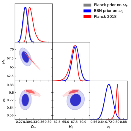
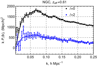
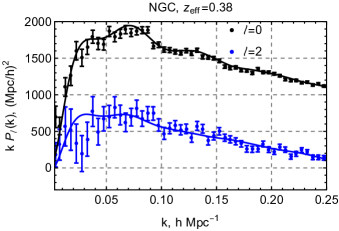
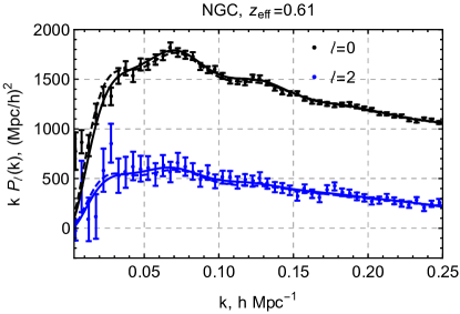
The outcome of our analyses is shown in Fig. 1, where we display the final triangle plot (left panel) and best-fit spectra for two BOSS data samples with the biggest volume101010These are high-z and low-z north galactic cap (NGC) samples. (right panel). The inferred cosmological parameters are given in Table 1. We have chosen to present the parameters , and as our main results because they are more common in the LSS literature and because they are close to the actual principal components of the BOSS data.
Our constraints on and are competitive with the Planck measurements for the same cosmological model with varied neutrino masses.111111There are several caveats that should be mentioned at this point. First, we approximate the neutrino sector with one massive eigenstate, which should be contrasted with the approximation of three degenerate eigenstates used in Planck 2018. The difference between these two approaches is a few percent at the matter power spectrum level, and hence can be neglected for our purposes. Second, the Planck Legacy contours that we show roughly correspond to the variation of the total neutrino mass in the range () eV, which is somewhat different from our prior () eV. However, the effect of weighting the Planck posterior with our prior on is marginal. We show the original Planck contours for clarity. Moreover, the use of the full parameter likelihood adopted in this work allows for a clear comparison between the two experiments at the level of the fundamental CDM parameters. Our measurement of is driven by the geometric location of the BAO peaks, whereas the limits on result from the combination of both the geometric (distance) and shape information. is measured through redshift-space distortions. We performed several tests to ensure that our constraints are saturated with these three effects, and confirmed that distance ratio measurements implemented through the Alcock-Paczynski effect can only marginally affect the cosmological parameters of CDM. However, the situation changes in its extensions that modify the late-time evolution, in which the Alcock-Paczynski effect becomes a significant source of information to constrain the parameters of these models.
In order to explore the relation with the previous works on the galaxy power spectrum we ran an analysis with very tight shape priors and obtained essentially the same results as in Tab. 1. However, in that case cannot be viewed as an independently measured parameter, since the shape priors completely fix the relation between and in CDM. This suggests that the shape priors are not necessary for the parameter estimation from the BOSS data. Moreover, the power spectrum shape itself can be a source of independent measurements of and , whose precision rivals that of the Planck CMB data. This happens because of two main reason. First, the parameter can be measured directly from the shape of the galaxy power spectrum with precision. Second, the degeneracy direction corresponding to the angular acoustic scale of the galaxy power spectrum happened to be more orthogonal to than the angular acoustic scale of the CMB. Thus, even though the later is measured with Planck much more precisely than the former one, their projections onto the plane happened to be comparable. In Section 5 we give some further details on this effect.
Our results agree with the Dark Energy Survey (DES) data on weak lensing and photometric galaxy clustering [50]. The combination best constrained by DES is within 2 of our limit .
Let us comment on the neutrino masses. Our analysis shows that the BOSS data itself can only rule out very large neutrino masses eV, which produce significant scale-dependent modifications to the matter power spectrum. These modifications are not degenerate with effects of other cosmological and nuisance parameters. Smaller neutrino masses cannot be constrained with the BOSS data mainly because of the degeneracy between galaxy bias and , which persists even if we use the Planck 2018 prior on . Naively, this degeneracy may be broken by the quadrupole moment, but its large statistical error along with the strong sensitivity to the finger-of-God uncertainties do not allow us to derive constraints on the neutrino mass that could be competitive with the CMB data. Note that the degeneracy between , and the galaxy bias can, in principle, be alleviated by the bispectrum data [51, 52].
To estimate results from a combined Planck + BOSS likelihood we analyzed the BOSS data with a multi-variate Gaussian prior on all cosmological parameters of the minimal CDM (not including the neutrino mass) from the final Planck data release [44]. We obtained the following limit from the combination of the two biggest BOSS data samples:
| (2.1) |
This suggests that the BOSS data can only improve the current neutrino mass bounds by breaking degeneracies internal to the CMB data (e.g. the degeneracy between and ), and not by actually observing the free-streaming short-scale suppression of the galaxy power spectrum [53]. It would be curious to see if the full-shape BOSS + Planck data will give better constraints than the Planck + BAO likelihood.
Finally, we tested some simple extensions of our baseline analysis, which assumes a BBN prior on and fixes the power spectrum tilt . To that end we explored the whole likelihood with all relevant parameters (). We have found that varying the tilt in chains with the BBN priors on degrades the constraint but does not significantly alter the and limits. Moreover, one can obtain a constraint on , which is independent of the Planck CMB data,
| (2.2) |
Instead, if we keep fixed but use a very wide prior on , the constraints on worsen by a factor of two, but the limits on and remain essentially intact. This suggests that our main conclusions are stable w.r.t. different prior choices.
3 Methodology and Likelihood
In this Section we discuss technical aspects of our analysis: the theoretical model, window function treatment, covariance matrices and model parameterization.
3.1 Theoretical Model
Our model for multipole moments of the redshift-space galaxy power spectrum is based on one-loop perturbation theory. Schematically, it can be written as a sum of four pieces,121212We use the following convention: , where we introduced the density (contrast) field ( and are the local and background densities, respectively), and denotes the averaging over the cosmological ensemble.
| (3.1) |
In this work we limit ourselves to the monopole and quadrupole moments (). All multipoles are computed from the 2D anisotropic galaxy power spectrum ,
| (3.2) |
where is cosine of the angle between a Fourier mode and the line-of-sight direction , whereas are Legendre polynomials of order . For example, the tree-level contribution to the multipoles are given by the Kaiser formula [54],
| (3.3) |
where is the scale-independent linear bias coefficient. For compactness, we suppress explicit time dependence in all formulas of this section assuming that all relevant quantities are evaluated at the effective redshift of a given data sample. For clarity, all the expressions of this section are presented without IR-resummation and the Alcock-Paczynski effect, which are properly taken into account, see Appendix A for more detail.
The next important ingredient of our analytic model is one-loop corrections that encapsulate the non-linear redshift-space mapping along with non-linearities due to dark matter clustering and bias. This model has been described in detail in Refs. [18, 55, 56] and is summarized in Appendix A. We use the following basis of bias operators131313As pointed out in [14, 57] the evolution of biased tracers is non-local in time, which leads to appearance of bias operators that cannot be written in terms of tidal tensor at a finite time slice. However, these operators appear only at fourth order in perturbation theory and this important subtlety is not relevant for the one-loop power spectrum that we consider.
| (3.4) |
where is the nonlinear matter density field and the Fourier representation of the tidal field operator is given by
| (3.5) |
where is the linear theory density field. Note that there is one extra bias parameter that contributes to the one-loop power spectrum, . We have found that this parameter is very degenerate with other nuisance parameters and the BOSS data are not accurate enough to break this degeneracy. For the purposes of this paper we have fixed it to zero. This choice still allows for a sufficient freedom in the parameter space exploration. We have checked that fixing or varying it within some priors has no effect on the cosmological parameter estimates.
The stochastic contribution is modeled as a simple Poisson shot noise with the constant power spectrum in Fourier space and a free amplitude. Note that in the absence of the window function only the monopole moment has a constant shot noise power, i.e.
| (3.6) |
Finally, the last part of our model are the so-called ultraviolet (UV) counterterms . The counterterms were not included in theoretical models used in the previous data analyses. For this reason, we discuss them in more detail here. The purpose of the counterterms is to fix the dependence of the one-loop power spectrum on the complicated unknown short-scale physics, which cannot be modeled by means of perturbation theory. To understand qualitatively why these corrections are needed let us note that a part of the loop integral comes from integrating over high- Fourier modes for which perturbation theory does not apply. This means that results of loop calculations are necessarily wrong, even though they converge to some finite values. For the theory to be consistent, there must be counterterms to cancel the spurious UV-dependence. Besides, standard perturbation theory does not correctly capture the backreaction of short scales on long-wavelength fluctuations. These effects are taken into account by the so-called “finite” part of the UV counterterms, which describes physical effects missing in standard perturbation theory. Since the loop integrals converge for the CDM linear power spectrum, there is no practical need to distinguish between these two physically different parts of the counterterms. Hence, every counterterm can be parametrized by a single free coefficient to be fitted from the data. Note that the scale-dependence of the counterterms is not free. It is fully fixed by symmetry arguments at any order in perturbation theory. This statement holds true for pure dark matter [11], dark matter halos [14, 16], and galaxies in redshift space [17, 18].
At first non-trivial order in the gradient and field power expansion there are two counterterms needed for the one-loop monopole and quadrupole moments [17, 18], which can be cast in the following form:
| (3.7) |
The reason to keep two different free coefficients is that they fix different loops and capture different physical effects. For instance, the monopole counterterm includes the contribution of the higher-derivative bias term , which is absent for higher moments. This should be contrasted with the quadrupole counterterm, which is dominated by the fingers-of-God effect [58]. Indeed, neglecting other nonlinearities, the -contribution can be related to the short-scale galaxy velocity dispersion ,
| (3.8) |
where we assumed and typical for the high-z BOSS sample. This formula is derived by expanding the velocity field into the short and long-wavelength contributions and averaging the redshift-space power spectrum over the short-scale modes,
| (3.9) |
which is then matched to our expression for . Note that a similar expression can be obtained upon Taylor-expanding some simple phenomenological models for the fingers-of-God with a Gaussian or Lorentzian damping, e.g. [59, 6, 5]. The typical value for the velocity dispersion for the BOSS-like sample Mpc yields . We emphasize that this is just a simple order-of-magnitude estimate and that the true amplitude (and even the sign) of the counterterms cannot be predicted.
The one-loop perturbation theory model (3.1) is sufficient to describe the statistics of biased tracers in real space up to for the volume and redshifts typical to the BOSS survey [60]. While two-loop contributions due to dark matter clustering may be sufficiently small, the mapping from real to redshift space can produce significant correction to the one-loop result because of higher order short-scale velocity cumulants, whose characteristic momentum scale can be significantly lower than the non-linear scale controlling gravitational non-linearities. This implies that the usual one-loop power spectrum model [17, 18] is not sufficient for an accurate description of the data even on large scales. One option to get around is to use some phenomenological model for the fingers-of-God. However, these models are not derived from first principles and can introduce uncontrollable biases in cosmological parameter estimations. To proceed, we choose a different strategy which fits the spirit of perturbation theory. We introduce an additional counterterm to capture the redshift space non-linearities at next-to-leading order (NLO),
| (3.10) |
Let us discuss the form of this expression. As argued above, the non-linear scale for the velocity dispersion is smaller than the dark matter nonlinear scale , but the stochastic velocity field couples with the large-scale density dominantly along the line-of-sight. Thus, the redshift-space mapping effectively generates an expansion in powers of . The standard one-loop counterterms in Eq. (3.7) correspond to the term in this expansion. From this point of view, the NLO counterterm in Eq. (3.10) can be naturally viewed as a next-to-leading term in this expansion, i.e. contribution.
It should be stressed that the main objective of introducing the new counterterm (3.10) is to capture the NLO sensitivity to fingers-of-God. The contributions from other physical effects (higher-derivative bias etc.) are expected to be sub-dominant since they have the same order of magnitude as the two-loop corrections to the real-space matter density. Thus, they can be neglected at the one-loop order that we use in this paper. Given this reason, we choose the NLO contribution (3.10) to be universal for all multipole moments, as expected from the redshift-space mapping.
Another way to understand role of the NLO counterterm is to view it as a simple model for the theoretical error. Marginalizing over the amplitude , we are marginalizing over the estimated uncertainty due to the fingers-of-God modeling. While in principle a more elaborate procedure is needed to ensure that the results of the analysis are unbiased [61], this simple prescription is sufficient given the BOSS survey volume.
In summary, our model for the power spectrum is based on one-loop perturbation theory for galaxies in redshift-space supplemented with LO and NLO counterterms. It includes seven free nuisance parameters: three bias coefficients (), three redshift-space counterterms () and the shot noise amplitude .
3.2 Power Spectra and Covariance Matrices
The BOSS survey has measured the spectroscopic redshifts of 1 198 006 galaxies using the SDSS multi-fibre spectrographs and multi-color SDSS imaging (see [62] and references therein). The BOSS-DR 12 galaxy sample spans over the redshift range . The data include four different selections: LOWZ, LOWZE2, LOWZE3, CMASS. They are combined into two non-overlapping redshift bins with and . Each redshift bin sample is additionally divided into two sub-samples depending on the Galactic hemisphere where the galaxies are observed. These are called “South and North Galactic Cap” (SGC and NGC). To avoid confusion with the previous selections analyzed, e.g. in [5], we will call the two redshift bins simply “low-z” and “high-z”. Note that each of the four data chunks has a different selection function and therefore represents a different galaxy population [62]. The comoving and effective volumes of the BOSS data samples are listed in Table 2. To obtain these numbers, the observed angles and redshifts were converted into comoving distances assuming the following fiducial parameters: , , which were also used to create galaxy catalogs.141414Throughout this paper we will use and the present day Hubble parameter km s-1Mpc-1 interchangeably. Any departure of the real cosmology from the fiducial one is accounted for by explicitly including the Alcock-Pazcynski effect in our theoretical model. The mean number density of each sample is approximately , implying that the shot noise is not a dominant contribution to the galaxy power spectrum on the mildly non-linear scales.
We use the redshift space power spectrum monopole () and quadrupole () of the publicly available data from BOSS DR12. The spectra are binned with the bin size in the wavenumber range . Our baseline analysis is performed for Mpc, which contains 50 -bins in each multipole. We have checked that our method can recover the correct cosmology from mock catalogs for this choice of (see Appendix B).
| Data | ||
|---|---|---|
| low-z NGC | ||
| low-z SGC | ||
| high-z NGC | ||
| high-z SGC |
Window function. We incorporate the effects of the survey geometry following the procedure described in [6]. The theory multipoles are first transformed to position space via
| (3.11) |
and then the corresponding correlation function multipoles are convolved with the appropriate window functions,
| (3.12) |
The windowed power spectrum multipoles are then simply obtained by means of an inverse Fourier transform,
| (3.13) |
The integrals in Eqs. (3.11) and (3.13) are computed with the FFTLog method [63].
Covariance matrix. We extract the covariance matrix from patchy mock catalogs, which are described in detail in Ref. [64]. The patchy algorithm is based on extended Lagrangian perturbation theory and a stochastic halo biasing scheme calibrated on high-resolution N-body MultiDark simulations run for a CDM cosmology with the following fiducial parameters:
| (3.14) |
The patchy algorithm uses halo occupation distribution (HOD) to construct catalogs which match the BOSS galaxy clustering and its redshift evolution. The patchy mocks were generated for every data chunk separately. In each case, they were assigned the same selection function and survey geometry as the real data.
We are using the covariance matrix extracted from the corresponding mocks,
| (3.15) |
where is the number of mock catalogs and is the mean power spectrum,
| (3.16) |
In our analysis we neglect the Hartlap factor correction [65] which affects the covariance matrix at the level of . For simplicity we will also defer from the standard practice of rescaling the parameter variances to account for the difference between the extracted values and the ones used in the mock catalogs [66]. A more accurate treatement of the covariance matrix would require its recalculation for the best-fit cosmology, which can be done analytically along the lines of [67].
3.3 Parameters and Priors
In all our analyses for the base flat CDM we vary 5 cosmological and 7 nuisance parameters:
| (3.17) |
where is the sum of neutrino masses, is defined as
| (3.18) |
and . Since each BOSS data sample has its own selection function, we allow biases, and counterterms for each data chunk to be different.
Let us discuss the choice of parameters and the corresponding priors. First, the initial conditions for fluctuations are described by two parameters, the amplitude of the power spectrum and the spectral index . The BOSS data can constrain the amplitude at level and the tilt cannot be measured with a reasonable accuracy. For this reason we fix the spectral index to be
| (3.19) |
as measured by Planck [44], and we do not vary it in the MCMC chains. This is why this parameter does not appear in (3.17). Since we cannot probe the amplitude of the primordial power spectrum accurately, our eventual results are not very sensitive to variations of the fiducial value of in a reasonable range around . In particular, all main results of our study would remain the same had we chosen the flat Harrison-Zel’dovich spectrum instead of (3.19). In App. C.2 we analyze the full power spectrum likelihood and show the effect of varying the tilt. As for the relative amplitude , we choose its prior to be uniform in the range .
Our final results will be presented in terms of the late-time mass fluctuation amplitude because (a) this parameter is better constrained than , (b) it is close to the actual principal component of the BOSS data and hence is less sensitive to prior choices, (c) it is more common in the large-scale structure literature. In Appendix C.1 we show results for both the rescaled primordial amplitude and .
As far as the neutrino sector is concerned, we approximate it with one state of mass and two massless states.151515This approximation is accurate for the matter power spectrum within precision for highest neutrino masses considered in this paper, which is sufficient for our purposes. Therefore, we will use and interchangeably in what follows. We assume a flat prior on in the range
| (3.20) |
The lower limit is inferred from the neutrino oscillation experiments and the upper limit is the 3 constraint obtained from the combination of the Planck 2018 TTTEEE+lowE+lensing data and the BAO scale measurements [44]. The BOSS data are not accurate enough to improve the measurement of the neutrino mass, hence we marginalize the final results over it. Nevertheless, it is important to keep this parameter in the chains since the neutrino mass is very degenerate with the amplitude of the power spectrum. Varying in the allowed range can bias the amplitude by the amount comparable to the error on this parameter. We have found that does not affect significantly the limits on and , which will be quoted as our final results.161616Note that our analysis constrains the late time fluctuation amplitude more directly than and this is why it is less sensitive to the neutrino mass. Specifically, we have repeated our analysis with no priors on the neutrino mass (), and found very similar results for the cosmological parameters, see App. C.3 for more detail. Even if we impose the Planck priors on all cosmological parameters, the neutrino mass can only be constrained at the level of 1 eV (95 CL), which is not competitive with other cosmological probes. Given this reason, we prefer to stick to the realistic prior allowed by other experiments and/or motivated by particle physics. The use of a somewhat wider prior eV matching the Planck 2018 2-allowed region has a negligible impact on our results.
Finally, assuming the flat CDM, the only additional cosmological parameters that are needed to describe the matter content of the Universe are physical densities of baryons and cold dark matter, and . The baryons have very distinctive effect on the CMB power spectrum, which allows one to measure their physical density with sub-percent accuracy [44] (assuming standard physics before and during recombination),
| (3.21) |
More conservatively, with minimal assumptions about the thermal and expansion history, the physical baryon density can be inferred using the BBN predictions and the measurement of helium and deuterium primordial abundances [68, 69, 44, 70],171717One may find different limits depending on nuclear rate predictions. Below we present constraints obtained using the helium data from [68], deuterium data from [69] and assuming , (3.22) The fist limit is obtained using the He nuclear rate from [71] and the PArthENoPE code [72]. The same code but a different nuclear rate taken from [73] yield the second constraint. Finally, using nuclear rates from [74] and the PRIMAT code (introduced in the same paper) gives the third constraint. In all the limits quoted above the systematic error is added in quadratures. We prefer to use the “standard” case in our analysis, although any other choice from (3.22) would produce very similar results. We are grateful to Julien Lesgourgues for sharing with us the limits (3.22).
| (3.23) |
We will see momentarily that both priors yield identical constraints for the BOSS data.
The physical density of cold dark matter can be also inferred from the shape of the CMB spectra with percent accuracy [44],
| (3.24) |
We will not use this prior in our main analysis, and vary in the flat range . The prior (3.24) will only be imposed in a side analysis that compares our method with the previous BOSS FS pipeline which also fixes .
As already pointed out, using the tight CMB priors on and effectively fixes the shape of the matter power spectrum and in this case our analysis reduces to the standard BOSS analysis. The only remaining difference is in the theoretical model used. This allows us to investigate the relation between our constraints on cosmological parameters and the previous BOSS results. It is worth noting that this choice of priors is equivalent to fixing a prior on the sound horizon at decoupling, since it can be approximated as [75],
| (3.25) |
where . Note that the sound horizon at the drag epoch is insensitive to the late-Universe physics [45, 76]. Planck gives a sub-percent measurement of this scale [44],
| (3.26) |
| Parameter | Prior |
|---|---|
| Cosmology | |
| (not varied) | |
| different for each analysis | |
| flat | |
| flat | |
| flat | |
| flat eV | |
| Biases and shot noise | |
| flat | |
| flat | |
| flat | |
| (not varied) | |
| flat | |
| Counterterms | |
| flat | |
| flat | |
Regarding the bias parameters, we adopt flat priors centered around the values expected from N-body simulations. The previous BOSS analyses have already measured , for which we use a flat prior in the range . The second order biases are varied in the range
| (3.27) |
These intervals are motivated by the measurements of biases for dark matter halos with masses similar to typical hosts for BOSS galaxies [77]. These measurements roughly predict181818Note that [77] use a different basis of biased operators. Their values have been appropriately converted to match our bias prescription.
| (3.28) |
The halo bias is in general different from galaxy bias, but given that the satellite fraction is relatively small in the BOSS samples [78], we expect these estimates not to be too far from the truth. In all analyses we set and we do not vary it. The reason for this choice is that is very degenerate with the counterterms , and . The data are not accurate enough to break this degeneracy. We have verified this using the mock catalogs.
Finally, let us discuss the amplitude of the shot noise. The number density of the galaxies in the BOSS samples is known, and it is roughly . However, one might expect some deviations from the Poisson value for the shot noise amplitude due to effects like exclusions [79]. Detailed comparisons to simulations [60] show that this deviation for BOSS galaxy number density is not expected to be very large (at most ). For this reason we will vary in the chains within the flat prior in the following range:
| (3.29) |
Another reason to vary the constant in our analysis is to capture the fiber collision effect. Indeed, this is a common practice to correct for the fiber collision residual contributions left after applying the nearest neighbor method [5, 6]. Ref. [80] pointed out that this practice is not sufficient for the quadrupole, which does not have a constant shot noise contribution. This reference showed that the problem can be alleviated by applying the effective window function supplemented with additional nuisance parameters, which correspond to a stochastic constant contribution for the monopole and a -contribution to the quadrupole. While the first term is accounted for precisely by , the second contribution happened to be fully degenerate with our NLO counterterm. We have checked that, to a precision of , the difference between the spectra with and without the effective window function can be absorbed into the nuisance parameters of our theory model. This difference is much below the statistical error and can be safely neglected, which is why we proceed without the effective mask.
All nuisance parameters, , and have the same priors in all our analyses. We summarize them in Table. 3. We use different combinations of priors on and in our analyses and we will specify them in each example separately.
Software. Our analysis is based on a modification of the publicly available CLASS code [43] that incorporates the FFTLog method [42] for fast evaluation of one-loop perturbation theory integrals. The parameter constraints are obtained with the April 2018 version of the Montepython code [45, 81]. Plots with posterior densities and marginalized limits are produced with the latest version of the getdist package191919 https://getdist.readthedocs.io/en/latest/ , which is part of the CosmoMC code [82, 83]. We monitor the convergence of our MCMC chains with the Brooks-Gelman and Gelman-Rubin criteria [84, 85]
4 Constraints on Base CDM
In this section we present measurements of parameters of the minimal flat CDM with massive neutrinos. Our final results are quoted in terms of , and since these parameters are most common in the large-scale structure literature. Another reason for the use of these particular parameters is that they are close to the actual principal components of the BOSS data202020E.g. the amplitude is very correlated with the neutrino mass, which degrades the relative error on compared to . Moreover, the asymmetric priors on make the posterior for very asymmetric as well. . Our main analysis does not assume CMB priors on (equivalently, ). We use several different priors on . These are the CMB prior (3.21), a slightly weaker BBN prior (3.23), and the CMB prior with a -times bigger variance. We impose the latter prior in order to check to what extent the prior is crucial for our results.
We start with the first case (the CMB prior on ). The reduced triangle plot with the relevant cosmological parameters for four different BOSS datasamples are shown in the left panel of Fig. 2. The full triangle plot and the 1d marginalized limits are given in Appendix C.1. There we also present results for parameters , , and , derived from our MCMC chains.
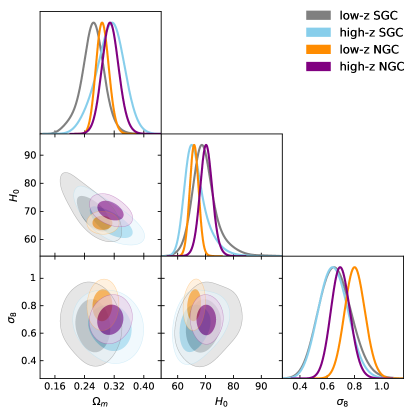
Let us first discuss the consistency of our results. The posterior distributions seen in the left panel of Fig. 2 overlap within 1 regions. The observed scatter is compatible with the hypothesis that all the independent samples are drawn from a single set of cosmological parameters. This suggests that these samples can be combined. The combinations of low-z, high-z, and all four samples are shown in the right panel in Fig. 2, while the corresponding 1d marginalized intervals are presented in Table 4. For comparison, we also show the Planck 2018 results from the TT,TE,EE+lowE+lowl+lensing data212121The MCMC chains for the base_mnu_plikHM_TTTEEE_lowl_lowE_lensing likelihood were downloaded from the Planck Legacy Archive http://pla.esac.esa.int/pla/#cosmology., which were derived for CDM with the varied neutrino mass. Overall, we observe good consistency between BOSS and Planck. The mean values of and inferred from different BOSS redshift bins are within distance from each other and from the Planck posterior mean values. One can notice that the high-z data prefer smaller than Planck. This tendency has already been observed in the previous BOSS full-shape analyses [86, 6]. However, the obtained difference between the Planck and our BOSS measurements is still consistent with a statistical fluctuation.
| Pl high-z | best-fit | mean |
|---|---|---|
| Pl low-z | best-fit | mean |
|---|---|---|
| Pl comb. | best-fit | mean |
|---|---|---|
| Pl | best-fit | mean |
|---|---|---|
The statistical errors of our and measurement are comparable with Planck errorbars for the parameters of the same cosmological model with massive neutrinos. Note that these parameters do not form principal components for the Planck data, and hence are relatively poorly measured, e.g. compared to the combination , which controls the angular position of acoustic oscillations in the CMB temperature power spectrum [87]. This fact is reflected in a well-known degeneracy between and , which can be clearly observed in the Planck contours shown in the right panel of Fig. 2. On the contrary, the degeneracy between these two parameters is not very strong in the BOSS data, which provide us with more direct measurements of and than Planck.
Our main conclusions remain exactly the same if we use the BBN prior on . Even in this case one can measure and quite well using no information from CMB whatsoever. Remarkably, our limit on the late-time matter density fraction is one of the best measurements of this parameter from the LSS data. We emphasize that this constraint is driven by the shape of the power spectrum. Since there is no difference between our measurements in the case of Planck and BBN priors on , we prefer to quote the latter ones as our final results because they use no input from the CMB data. The corresponding posteriors are shown in Fig. 1, and limits are displayed in Tab. 1.
To test the stability of our results we have run the same analysis assuming the Planck Gaussian prior on with a times bigger error (). In that case the BOSS data are able to deliver an independent constraint on . Still, this limit is by far superseded by the BBN, and will not be quoted here. Upon marginalizing over , we obtain the following constraints: , km/s/Mpc, . Remarkably, our measurement of did not degrade once we relaxed the prior on , whereas the measurement of worsened by a factor of 2. The stability of is consistent with the observation that upon marginalizing over the matter density forms a principle component of the geometric information is [56]. The degradation of occurs because it is mainly extracted from by using the power spectrum shape (which probes and ), which has less constraining power without the prior.
It is important to stress that so far we have not imposed a prior on . Moreover, since depends on and , our analysis provides an independent measurement of the acoustic horizon at decoupling, which is consistent with Planck,
| (4.1) |
To see how much this result depends on the prior, let us also quote the value obtained in the analysis with a loose non-informative Gaussian prior described in the previous paragraph,
| (4.2) |
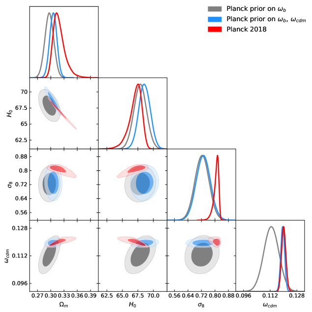
Now let us discuss the constraints obtained with the Planck priors on both the physical baryon and dark matter densities. As argued previously, in this case the shape of the matter power spectrum is only allowed to vary within very tight priors, thus for practical purposes the shape is effectively fixed. This case corresponds to the standard FS BOSS analysis.
Our results for the 2d posterior contours are shown in Fig. 3, while the 1d marginalized limits are quoted in the lower right corner of Tab. 4. One may notice that and have shifted upwards by w.r.t. our baseline analysis with the prior only, while their errorbars reduced only marginally. Obviously, in this case is a derived parameter which is almost fully correlated with . This should be contrasted with our baseline analysis without the prior, where is a valid degree of freedom. Remarkably, the prior has a marginal effect on and , which implies that this prior is not necessary for an accurate parameter estimation from the LSS data. This result is clear from Fig. 3, which shows that is not very degenerate with and . This effect will be discussed in more detail in Section 5.
Finally, let us discuss some implications of our results. Our measurement of is consistent with Planck [44] and the recent BAO + BBN analyses of Refs. [88, 70]. However, it is in tension with the results of the local astrophysical measurements of SNIa [89] and strong gravitational lensing of distant quasars [90]. Our study shows that the full-shape power spectrum information constrains at level, which is comparable to the SNIa limits. Since there is no prior in our analysis, it disfavors explanations for the “tension” based on modified expansion history at high redshifts which preserve the shape of the power spectrum, e.g decaying DM.
As for our constraint on , it is times worse than the Plank limit, but can be used to discriminate various proposals for the resolution of the tension that involve modifications of the linear power spectrum, such as early dark energy. We will explore this in more detail in a separate publication.
5 Geometric, Shape and Alcock-Paczynski Information
In this Section we quantify the information content of various effects relevant for the galaxy clustering data. To that end, we will first roughly classify all the relevant effect and then give some theoretical background on the difference between the geometric and the shape information. In the second part of this Section we will analyze several mock likelihoods mimicking the BOSS data in order to explicitly see how much different effects contribute to the final constrains. Throughout this Section, we will be working within base CDM and for simplicity assume that all neutrinos are massless.
The sources of cosmological information can be roughly classified into four categories:
-
•
Distance-free shape information. For a fixed , the power spectrum shape mostly depends on and (and , to a lesser extent), which control the relative amplitude of the BAO wiggles (through ), their frequency (through ), the amount of the short-scale suppression due to baryons (through ), and the relative position of the BAO wiggles and the baryon Jeans scale w.r.t the power spectrum peak (via222222We introduced an obvious notation . ). The relative shape does not depend on the choice of rulers (i.e. ).
-
•
Geometric (or distance) information. The features discussed above (e.g. the BAO frequency) can be assigned a (comoving) length scale for a given cosmological model, which constrains parameters of this model. Indeed, the position of the BAO wiggles in momentum space as extracted from the monopole is set by , where the effective “volume-averaged” distance is defined as232323We work in the unit system with .
(5.1) (5.2) Analogously, the location of the monopole power spectrum peak is set by . In CDM the physical densities of baryons and dark matter are fixed by the transfer functions, thus there is only one parameter , which controls the location of the power spectrum features.
-
•
Alcock-Pazcynski information.242424It should be pointed out that the division into “geometric” vs. “AP” information is somewhat artificial as these two effects cannot be isolated in a real survey. Alternatively, one may discuss the monopole vs. quadrupole distance information, see e. g. [91]. The radial and angular distances can be measured separately through the AP effect [37], parameterized by
This parameter in encoded in the power spectrum quadrupole. We will see that in CDM these distances are fixed by the shape and geometric information, but they can measured independently of this information in the extensions of CDM.
-
•
Redshift-space distortions. RSD help to measure the velocity power spectrum from the quadrupole power spectrum moment, which constrains . The shape and geometric information breaks the degeneracy between and (which mostly depends only on the background expansion, i.e. in CDM ).
Our main goal is to show how the first two effects contribute to our new constraints. Let us focus on them.
5.1 Shape vs. Geometry
In this Section we will discuss in more detail the shape information and its distinction from the distance information. This material will be somewhat pedagogical and has an overlap with old works on the galaxy clustering that were using the power spectrum shape for cosmological parameter measurements independent of CMB [92, 93, 94]. Unless otherwise stated, all numerical estimates of this Section will be made for the Planck best-fit CDM cosmology [44].
It is instructive to review the role of the shape and distance information from the CMB power spectrum of temperature (TT) fluctuations. The primary CMB spectrum has three main sources of information, which can be cast into the amplitude, shape and geometric distance. The latter two are the relevant ones for our discussion. They can also be loosely called the “horizontal” and “vertical” information [92]. Vertical information refers to the relative height of the acoustic peaks, i.e. their shape, which depends only on the physical matter densities and and the tilt . The distinctive physical effects produced by variations of these parameters allow to measure them regardless of any late-time physics [45, 46]. By horizontal information we mean the acoustic angular scale, which controls our freedom to shift the spectra in the horizontal direction (rescaling of angular multipoles ’s). The angular size of the sound horizon at the drag epoch is given by
| (5.3) |
(where and are the sound horizon at decoupling and the angular diameter distance corresponding to the decoupling redshift ). Although this single parameter has been measured by Planck with tremendous precision [44], it depends on multiple cosmological parameters. The numerator of (5.3) is a slow function of and (see Eq. (3.25)). However, the denominator depends sensitively on the late-time expansion. If one expresses the measurement of in terms of the late-time parameters and , one finds a strong degeneracy corresponding to fixed , with projections onto each separate parameter being much wider than this combination itself. The geometric degeneracy of the CMB gets eventually broken by the shape information of the power spectrum, i.e. by and being measured from the relative hight of the CMB peaks.
Analogously to the CMB, the angular position of the BAO in the monopole power spectrum of galaxies at some is given by
| (5.4) |
If one were to measure only the combination (5.4) just like in the BAO analysis, the degeneracy between and could not be broken and one would be left with the horizontal information only. However, it is precisely the shape (vertical) information that allows one to decouple and .
As discussed above, the sound horizon depends on , only (though very weakly, see Eq. (3.25)). These two parameters can be measured directly from the shape of the matter power spectrum regardless of the late-time expansion just like in the CMB case. To see this, we display in Fig. 4. the effect of varying these parameters. One clearly sees that and control the frequency of the BAO, the shape of the BAO wiggles, the amount of the short-scale suppression due to the baryon free-streaming before recombination, the overall slope of the power spectrum and its turnover. In the case of our baseline analysis with fixed and , all these effects depend only on one parameter , which results in quite tight constraints.
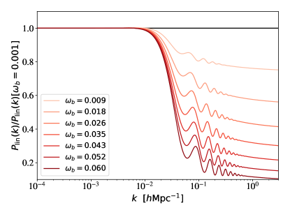
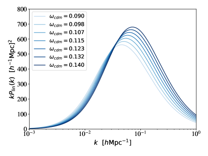
It is precisely the shape information on (and hence, ) that allows one to break the degeneracy between and and measure directly from . The crucial point is that in CDM is an extremely slow function of at small redshifts relevant for galaxy surveys. Indeed, using Eq. (5.1) one finds252525The Alcock-Paczynski effect also allows one to independently measure from the quadrupole. However, it turned out to be quite insensitive to either, . This shows that the low-redshift AP effect is a very weak probe of .
| (5.5) |
Since is absolutely fixed by the shape information, reduces directly to . Overall, the situation is very similar to the CMB temperature fluctuation spectrum, whose degeneracy gets broken by the vertical shape information. Crucially, the degeneracy direction between and in the galaxy BAO is more perpendicular to than that of the CMB acoustic scale, which results in better constraints even though at face value the precision of LSS measurement is worse than that of the CMB. This fact was pointed out long ago in Refs. [92, 93, 94]. Let us explicitly illustrate this. Using the expressions (3.25) and (5.1), we get
| (5.6) |
This implies that the acoustic peaks in the galaxy spectrum constrain the combination . A similar calculation carried out for the CMB acoustic peak (5.3) gives (see Ref. [87]). Clearly, unlike the CMB, the LSS acoustic angle is a very weak function of and hence it allows one to accurately measure .
Importantly, the galaxy power spectrum contains additional geometric information on top of the BAO wiggles. The first piece of this information is given by the angular position of the power spectrum peak,
| (5.7) |
The second piece of additional information beyond the BAO is given by the same sound horizon scale , which also marks the location of the baryon free-streaming scale (see the left panel of Fig. 4). Thus, in principle, one could derive constraints on and even if the BAO were not present in the matter power spectrum. This point will be illustrated in a mock data analysis of the next subsection.
The power spectrum peak (turnover) itself gives a complementary way to break the degeneracy between and . Indeed, one can notice that the two angular scales (5.4) and (5.7) have very different sensitivity to and . Indeed, the BAO angle constrains . However, the power spectrum turnover fixes a combination ,
| (5.8) |
Therefore, the following two combinations of these angles would directly measure and ,
| (5.9) |
This shows that even in the case where the measurement of from the slope is complicated by marginalizing over the power spectrum tilt (see App. C.2), can still be inferred from the power spectrum peak.
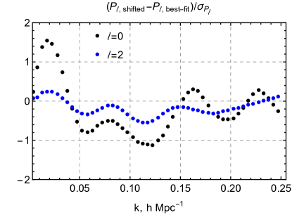
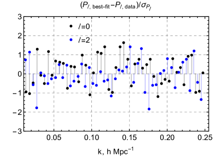
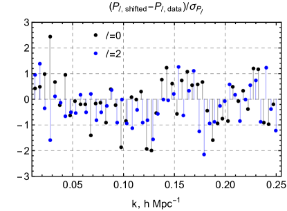
Finally, in order to get convinced that our constraints are indeed driven by the shape we have performed the following exercise. We have taken the best-fit power spectrum from the NGC high-z datasample (which has the biggest volume) and compared it to the spectrum computed for a model with shifted by away from the best-fit value. At face value, this leads to an extremely large difference in because enters various normalizations. However, much of this difference is absorbed into the nuisance parameters and cosmological parameters. Thus, we have refitted all the parameters of the “shifted” trial model. The results are shown in Fig. 5, where one can see the two trial spectra and the difference between them in terms of the statistical error on the power spectrum . The difference between values of the two models is . Clearly, the variation in is detectable. It cannot be undone by a simple shift in : either the BAO wiggles or the slope will be wrong.
5.2 Mock data analysis
In this Section we will be mainly focused on disentangling the shape, geometry and AP information, which are most relevant for the constraints on and . To quantify the amount of information coming from them we analyze several mock BOSS-like likelihoods. We use our theoretical pipeline to generate datavectors for a random set of cosmological and nuisance parameters extracted from the MCMC chains for the low-z NGC mocks.262626These are: . Note that these parameters are within 1-distance from the fiducial values used in mock catalogs. We analyze these mock spectra using the same pipeline in order to obtain the reference posterior distribution. We assume the same priors as in our main analysis (see Tab. 3), and additionally put the following Gaussian prior on :
| (5.10) |
which is equivalent to the BBN (or Planck) prior on used in our baseline analysis, but centered at the fiducial value used in the mocks. The reference posterior contours are shown in Fig. 6, the 1d marginalized limits are given in Table. 5. Note that they match the results of our analysis of the mock catalogs and the real data for the same data chunk.
| Reference | best-fit | mean |
|---|---|---|
| only | best-fit | mean |
|---|---|---|
| Fake AP | best-fit | mean |
|---|---|---|
To estimate the information content of the BAO wiggles, we generate and analyze a datavector without them. A similar approach was previously employed in Ref. [95, 56]. To that end we use the same wiggly-smooth decomposition procedure that performs IR resummation. These mock non-wiggly data are then analyzed with a modified pipeline that does not have the BAO wiggles in theoretical template too.272727We emphasize that we only removed the BAO wiggles from the power spectrum templates. All other baryonic effects, e.g. the Jeans suppression, are present in our theory model. The results of this analysis and the reference posteriors are shown in Fig. 6. The 1d marginalized limits are given in Table. 5.
First, we see that the constraints on are similar in the BAO and no-BAO cases. This means that the BAO wiggles represent only a part of the shape information. However, their presence is crucial for constraining through the geometric information. To see this, let us focus on the degeneracy directions seen in the panel. These are for the no-BAO case and with the BAO. The first one exactly corresponds to the power spectrum shape (or the location of the power spectrum peak in units Mpc/). The second one is likely a combination of the location of the power spectrum peak and BAO wiggles (set by , see (5.6)). As a consequence, in the realistic BAO case the projection of the degeneracy contour onto the plane is twice more narrow compared to the no-BAO contour. We point out once again that in the BAO case the principle component of the geometric information happens to be quite perpendicular to , which explains why this combination of and is well constrained. Once we remove the BAO, the principal component changes and the projection onto the plane becomes twice larger than before.
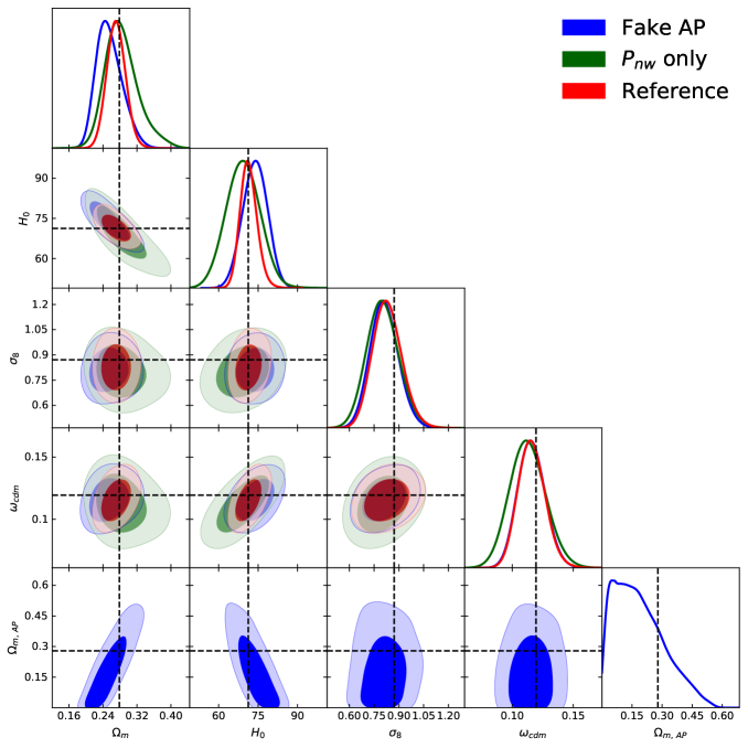
Now let us focus on the Alcock-Paczynski information. To quantify its amount we take the reference datavector with the BAO wiggles and analyze it assuming the matter density fraction that enters the geometric distances and the AP effect to be different from the true . Technically, it is equivalent to considering a model where the late-time geometric expansion is controlled by an additional parameter, which is not related to the ones fixing the shape of the matter power spectrum. We use the following flat prior on :
| (5.11) |
The outcome of this analysis is also displayed in Fig. 6 and in Table. 5 (“fake AP”). One first notices that the constraints on are identical in the reference and the “fake AP” cases, which implies that the shape information is not diluted by the AP distortions. This result explicitly proves our intuition that is measured directly from the power spectrum shape regardless of the late-time expansion.
However, since the location of the BAO wiggles mainly constrains , the presence of an additional parameter entering makes it harder to translate this constraint directly to . This explains why the constraints on the physical and degrade by . These limits, however, are not significantly worse than the reference ones because the degeneracy between and gets eventually broken by the quadrupole, which essentially constrains in our example.282828To be more precise, the quadrupole constrains the combination evaluated with instead of actual . The reason why the coupling between and does not dramatically worsen the measurement is that has a very weak sensitivity to the redshifts of interest, and at leading order292929At first non-vanishing order in one finds . even in our unphysical example with . Note that the posterior distribution of is highly asymmetric; its upper limit is set by the quadrupole information (which decouples and from ), while the lower limit is prior-driven.
The upshot of this discussion is the following. Our constraints on are driven by the power spectrum shape, is set by the geometric information (extracted from ) and is a combination of the two. As for the AP effect, it is absolutely superseded by the shape and geometric information in CDM. The situation is different for extensions of the minimal CDM, which we discuss now.
6 Distance Measurements
This section has three main objectives:
(a) establish the connection between our method and the one commonly used in the previous BOSS full-shape analyses with scaling parameters (-analysis in what follows),
(b) show that our analysis with the Planck priors on is equivalent to the -analysis if one takes into account that and are coupled in CDM,
(c) show that the -analysis is valid if one wants to constrain some generic late-time expansion models, for which the distance measurements become a leading source of information.
The analyses performed in this section have a demonstrative character. They aim to illustrate the relation between our method and the -analysis in different settings. We present results obtained for the BOSS NGC data samples only.
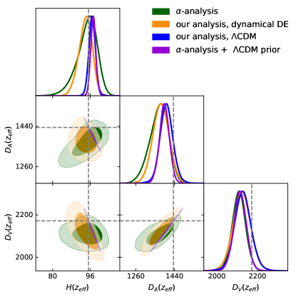
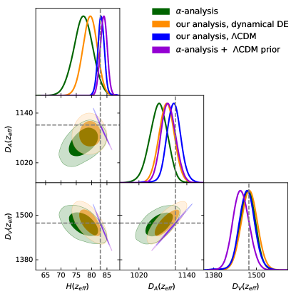
For the purposes of this Section we have run an -analysis using the same methodology as the previous BOSS FS studies. The details of this analysis are given in Appendix D. The -analysis computes the PS shape for a Planck-like cosmology and does not vary it in the MCMC chains. The main idea behind the -analysis is that once the physical densities of dark matter and baryons are fixed, the leading response to a change in cosmological parameters should be through and . However, fixing the shape is equivalent to fixing and , which also fix . Hence, the -analysis and our method should technically coincide if we fix in the -analysis and in our analysis. We stress that unlike the pure BAO-studies, fixing the shape and treating as a free parameter in the full-shape studies is unphysical. In any realistic model and the transfer functions’ shape are controlled by the same parameters. Thus, the -analysis of the full-shape power spectrum actually measures the absolute distances and and not or , which would be the case for the BAO-only study.
Another important observation is that the -analysis assumes and to be completely independent from each other, while in reality they are related by construction, see Eq. (5.2). In CDM a prior on and completely fixes the relation between and at any redshift. Once we impose this relation,303030To that end we have run mock MCMC chains that fitted and from the Gaussian likelihood for assuming CDM. Then we found the principal component of these variables and imposed this as a prior in the MCMC chains which sampled parameters. the limits on and from the -analysis coincide with the limits obtained with our method (modulo some small difference which can be explained by the use of slightly different priors and theoretical models, see App. D for more detail). This can be seen in Fig. 7 and Tabs. 7, 7.
| -parm. | best-fit | mean |
|---|---|---|
| -parm.CDM | best-fit | mean |
|---|---|---|
| DEE | best-fit | mean |
|---|---|---|
| CDM | best-fit | mean |
|---|---|---|
| -parm. | best-fit | mean |
|---|---|---|
| -parm.CDM | best-fit | mean |
|---|---|---|
| DDE | best-fit | mean |
|---|---|---|
| CDM | best-fit | mean |
|---|---|---|
One can notice that the CDM priors have a very dramatic effect on the measurements of and , whose errorbars reduce by a factor of few compared to the basic -analysis without any priors. However, the effect on is not very strong.313131It is useful to compare our limits with the ones obtained in the main BOSS Fourier-space BAO and FS power spectrum analyses, see Refs. [6, 96]: Note that these limits were obtained by using slightly different datasamples (NGC+SGC), cuts and the theoretical model, and hence should be compared to our results shown in this section with some caution. This reflects the observation that is the best measured combination of and , which is extracted directly from the monopole, while and are measured from the quadrupole, which has significantly larger statistical errors and features much less pronounced BAO wiggles. In other words, our analysis shows that the good constraints on and obtained in CDM are prior-driven, these two parameters are not measured directly. is the only one actually measured prior-independent distance in CDM.
In order to explicitly illustrate that the principal distance best measured from our analysis is always given by even in extended cosmological models, we analyze the BOSS data assuming a generic dynamical dark energy (DDE) model, described by the following Friedman equation:
| (6.1) |
We assume the following flat priors on and :
| (6.2) |
and keep the Planck priors on and . As far as the other cosmological and nuisance parameters are concerned, we use the same priors as in our baseline analysis, see Tab. 3. Note that a model similar to (6.1) has been constrained in the previous BOSS analyses, e.g. [62].
The results for the NGC high-z and low-z data are presented in Fig. 7 and Tables 7, 7. The first relevant observation is that the background parametrization (6.1) is sufficient to decouple the radial and angular distances, so that the errorbars on and become comparable to the ones obtained with a generic -analysis, and these two distances are not noticeably degenerate. The second important observation is that the limit on is the same as in the CDM case, which confirms that is an actually measured distance that forms the principal component. Importantly, the relative precisions of its measurement from separate chunks are (low-z NGC) and (high-z NGC), which is comparable to our precision on in the CDM analysis. The comparison between the DDE and CDM cases presented in Tabs. 7, 7 allows us to conclude that our precision on in CDM indeed originates from the precise measurements.
As far as the angular diameter distance is concerned, its errorbars are the same in two models, but the mean values are noticeably shifted compared to the CDM case. This shows that is fixed by the shape and geometric information in CDM, but can take different values in the non-minimal extensions of this model.
Our measurement of and in the DDE model are prior-driven, as can be deduced from comparing the corresponding contour with the one obtained from the -analysis, which did not assume any priors.323232The limits on the parameters of the DDE model are also prior-dominated, which is why we do not quote them here. Indeed, the -analysis reveals a clear degeneracy between and that corresponds to fixed , while our DDE posterior does not show any significant degeneracy between and whatsoever. This merely reflects the fact that the quality of the quadrupole measurement is not good enough for a decent determination of these distances separately. This is why our MCMC sampler hits the prior boundaries before it starts seeing the degeneracy. Finally, it is worth pointing out that the constraints on degrade significantly in the DDE model compared to the CDM case as a consequence of increased parameter space, which cannot be constrained using the available distance information.
Our study suggests that the model-independent -parameterization might be too generic for some purposes. Indeed, even in the case of a very general DDE model with quite loose priors on its parameters (6.2) we were not able to cover all the parameter space sampled by the -analysis. Hence, one always has to impose proper priors on the -parameters in order to use the distance information for precision constraints on non-minimal cosmological models. This is important for consistency when combining the BAO/FS data with external likelihoods (e.g. CMB, SNe or weak lensing) that assumed certain priors on the CDM extensions, e.g. [44].
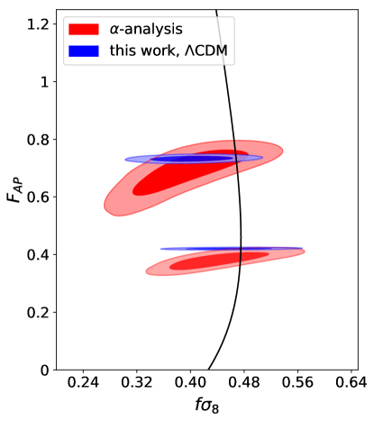
Finally, let us briefly comment on the so-called Alcock-Paczynski parameter,
| (6.3) |
which is often used to present the results of galaxy clustering measurements. By construction this quantity depends only on in CDM. One can easily check that by definition must be roughly equal to at low redshifts, where all cosmology dependence essentially cancels. However, even for the BOSS high-z effective redshift has only a logarithmic dependence on . Thus, the use of this quantity for comparison might be misleading, since in CDM it always has a very small error because of a negligible small sensitivity to cosmology. This is illustrated in Fig. 8, where we show the diagram extracted from our MCMC chains for the base CDM. The situation changes in extensions of CDM, where can reflect some non-trivial information.
7 Conclusions and Outlook
We have presented new limits on the cosmological parameters of the minimal CDM from the BOSS DR12 on the anisotropic redshift-space galaxy clustering. Our study features several important improvements. They include the use of a complete theoretical model for the non-linear power spectrum and the MCMC technique for parameter inference. In contrast to previous Fourier-space galaxy clustering analyses of the power spectrum multipoles [86, 5, 6], we consistently recompute the full likelihood as we sample different cosmological and nuisance parameters.
Our analytic model for the galaxy power spectrum is based on one-loop perturbation theory. It includes the non-linearities in the underlying dark matter field, bias expansion, and redshift-space mapping. In addition, it properly takes into account the damping of the BAO produced by large-scale bulk flows, which is described by means of IR resummation. Finally, our model incorporates corrections due to backreaction of short-scale modes, which cannot be reliably modeled within perturbation theory itself. These effects are captured by a number of so-called “counterterms,” whose shape is fixed by symmetries and whose amplitude is characterized by free coefficients, which are treated as nuisance parameters in this work. Another feature of this work is the use of the novel FFTLog algorithm [42], which made computations of the non-linear galaxy power spectra and related likelihoods highly efficient and robust. We implemented this algorithm in the Boltzmann code CLASS [43], which enabled us to quickly produce theoretical templates for a given cosmology. This code can be easily interfaced with common cosmological MCMC samplers like Montepython [45, 81] or cobaya333333 https://github.com/CobayaSampler/cobaya . Thus, the present work is the first practical application of many recent efforts in large-scale structure theory.
The main outcome of our work is that the so-called shape priors are not actually necessary in the full-shape power spectrum analysis. The BOSS power spectrum data alone can be used to constrain the late-time matter density and the Hubble parameter with precision similar to that of the Planck CMB measurements. Our study shows that the power spectrum shape contains a considerable amount of information in addition to the BAO wiggles and the Alcock-Paczynski distortions, which were the main focus of previous anisotropic galaxy clustering analyses. We stress that even though our baseline analysis does not directly use the CMB data, it assumes informative priors on the power spectrum tilt, the physical baryon density, and the total neutrino mass. On the one hand, they can be seen as theoretical priors strongly motivated by the CMB measurements. On the other hand, they can be viewed as a minimal input from the CMB, which allows one to fix some degeneracies poorly constrained by the BOSS data itself. In this regard, our baseline priors are similar, by spirit, to the FIRAS prior on the CMB monopole temperature, and the minimal neutrino mass allowed by the oscillation experiments, which are the key external priors used to constrain the base Planck CDM model [44].
The parameters of CDM measured in this work are consistent with the results of the Planck CMB observations [44] and the DES survey [50]. It would be interesting to see how much the cosmological parameter constraints can be improved by combining the data from these experiments with our full-shape power spectrum likelihood. Our method can also be easily applied to the eBOSS quasar clustering data [97, 98].
The main factor limiting the range of scales used in our analysis was the fingers-of-God effect. This effect forced us to increase the number of nuisance parameters and eventually prevented us from employing the modes with comoving wavenumbers bigger than . We believe that this problem can be alleviated by using the redshift-space wedges [7], which can extend the regime of validity of our theoretical model without having to compute higher-order corrections. Another aspect that requires improvement is the covariance matrix treatment. Ultimately, it is desirable to use an analytic expression which can be easily recalculated for a new cosmology e.g. if the estimated cosmological parameters happen to be different from the ones used to generate the covariance matrix for the initial analysis. The validation of our results with different covariance matrices represents a necessary consistency check. Finally, it would be interesting to see how the analysis can be improved by including the theoretical error, e.g. [61, 56]. These questions are left for future investigations.
Note added. When the CLASS module for fast perturbation theory calculations used in this paper was being developed, we became aware of the work [99], which was applying a similar theoretical model to analyze the BOSS data. This inspired us to use our code for the BOSS data analysis. We thank the authors of [99] for discussions and sharing with us their preliminary results. The methodology and theoretical model used in Ref. [99] are very similar to ours, but the numerical implementation is completely different. Note that compared to us, Ref. [99] uses slightly different data selections and prior choices. When overlap, our results agree.
Acknowledgments
We are indebted to Florian Beutler for providing access to the BOSS DR12 measurements and various related products, and to Roman Scoccimarro for sharing with us the power spectra from the LasDamas N-body simulation.
We would like to thank Guido D’Amico, Jonathan Blazek, Anton Chudaykin, Elisabeth Krause, Julien Lesgourgues, Antony Lewis, Ariel Sanchez, Alvise Raccanelli, Leonardo Senatore, Blake Sherwin, Zvonimir Vlah, and Jay Wadekar for useful discussions. We are grateful to Colin Hill, Sergey Sibiryakov, Uro Seljak, Masahiro Takada, and Benjamin Wallisch for comments on the preliminary version of this paper. All numerical analyses of this work were performed on the Helios cluster at the Institute for Advanced Study. M.Z. is supported by NSF grants AST1409709, PHY-1521097 and PHY-1820775 the Canadian Institute for Advanced Research (CIFAR) program on Gravity and the Extreme Universe and the Simons Foundation Modern Inflationary Cosmology initiative. M.I. thanks the CERN Theory Department and MIAPP Munich for hospitality during the completion of this work. M.I. acknowledges the support from the Swiss National Science Foundation and the RFBR grant 17-02-00651 at the initial stages of this work. M.I. is partially supported by the Simons Foundation’s Origins of the Universe program.
Appendix A Theory Model
Our model for galaxy power spectrum in redshift space is given by
| (A.1) |
where the redshift-space kernels are given by [22],
| (A.2a) | |||
| (A.2b) | |||
| (A.3) |
where and the kernel has to be symmetrized over its arguments.
Now let us discuss our implementation of IR resummation. We follow the approach streamlined in Refs. [28, 30], which was developed in the context of time-sliced perturbation theory [100]. IR resummation splits the matter linear power spectrum into the smooth and the wiggly parts,343434In practice, we use the wiggly-smooth decomposition technique introduced in Ref. [95].
| (A.4) |
where is a broadband power-law function, and contains the BAO wiggles. The IR resummed anisotropic power sepectrum at leading order takes the following form,
| (A.5) |
where we introduced the anisotropic damping factor,
| (A.6) |
that depends on the following contributions
| (A.7) |
is the BAO wavelenght Mpc, is the separation scale controlling the modes which are to be resummed, and are the spherical Bessel function of order . In principle, is arbitrary, and any dependence on it should be treated as a theoretical error. Following [28] we define it to be /Mpc, which gives the same result as an alternative choice , adopted in [26].
In general, IR resummation in redshift space at next-to-leading (one-loop) order requires a computation of anisotropic loop integrals which cannot be reduced to one-dimensional ones. One can simplify these integrals by splitting the one-loop contribution itself into a smooth and wiggly part. More precisely, one first computes the one-loop integrals with a smooth part only. At a second step one evaluates these integrals with one insertion of the wiggly power spectrum and suppresses the output with a direction-dependent damping factor (A.6) to get
| (A.8) |
where is treated as a functional of the input linear power spectrum, and
| (A.9) |
The IR-resummed anisotropic power spectrum should then be used to compute the multipoles in Eq. (3.2).
To account for the AP effect one has to compute the observable galaxy power spectrum,
| (A.10) |
where and are related to wavevectors and angles in the true cosmology, whereas and refer to quantities obtained for a given set of assumed cosmological parameters. The relation between the true and observed wavevectors is given by
| (A.11) |
During MCMC analysis one tries to find and given and that are fixed by the reference cosmological model used to create galaxy catalogs. The eventual galaxy multipoles with the AP effect are given by
| (A.12) |
Appendix B Tests on Mock Catalogs
In this Appendix we show the tests of our pipeline on mock catalogs. First, we will apply our pipeline to the high-resolution mock catalogs based on the N-body simulation LasDamas, which are characterized by the gigantic volume of ( (Gpc)3). These are mocks of Luminous Red Galaxies that are desinged to match the sample observed by SDSS [101]. Second, we will test our pipeline on MultiDark patchy mock catalogs [64]. On the one hand, they are based on approximate gravity solvers and HOD models. On the other hand, they are designed to closely reproduce the data and have the same selection, window function, and fiber collision effects implemented.
B.1 Tests on LasDamas N-body simulations
We will fit the monopole and quadrupole of the galaxy power spectrum of LasDamas Oriana simulations at redshift . This redshift is lower than the ones used in our analysis and therefore it provides a more stringent test of our theoretical model because the non-linear effects are stronger. The cosmological parameters used to generate mock catalogs are , , , , , and . The details of LasDamas simulation can be found at.353535 http://lss.phy.vanderbilt.edu/lasdamas/overview.html
We fit the mean of power spectra extracted from 40 independent simulation boxes, whose volume is each. This totals to (Gpc/)3 volume, which is almost 100 times bigger than the cumulative volume of BOSS. However, the statistical error corresponding to this tremendous volume is so small that the two loop corrections supersede cosmic variance already on very large scales. The situation is different for low-volume surveys like BOSS, where the statistical error is expected to be bigger than the systematic one down to very high . Hence, in order to be realistic, we will assume a covariance that corresponds to the BOSS survey and not to the actual Las Damas volume. Since 40 realizations are not enough to accurately estimate the covariance, we will use a theoretical prediction obtained in the Gaussian approximation (see, e.g. [56]),
| (B.1) |
where we introduced the number of modes , the binning step of Las Damas simulations /Mpc and the survey volume . Note that the monopole moment includes the shot-noise contribution, which is equal to [Mpc/h]3 for the LasDamas mocks. We will consider two particular choices,
| (B.2) |
is the total volume of the BOSS survey across all redshifts and sky parts, whereas is simply a 10 times bigger volume, which will be used to better pin down the theory systematic error. Using an approximate Gaussian covariance also provides an additional challenge to our approach: neglecting the off-diagonal terms artificially reduces the error and makes one reject the true model more often than it should be.
To make a closer contact to our analysis, we will keep and fixed to the true values and scan over , , in our analysis. We use the same nuisance parameters and assume the same priors for them as in our baseline analysis.
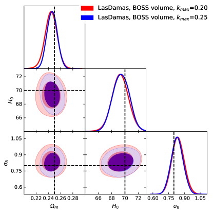
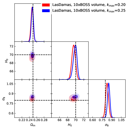
| best-fit | mean | |
|---|---|---|
| best-fit | mean | |
|---|---|---|
Our results are presented in Fig. 9 and in Table 8. In Fig. 9 we show the contours obtained for two choices of /Mpc and /Mpc. Table 8 displays the marginalized one-dimensional limits for /Mpc, which will be eventually selected as a baseline data cut.
Let us focus on the case corresponding to the total BOSS volume (left panel of Fig. 8). One can see that our pipeline correctly extracts the cosmological parameters within for both choices of . Remarkably, the errobars are very similar to the ones obtained in the analysis of the real data. The difference between the two choices of is marginal, which merely reflects the fact that the errorbars cannot be further improved due to the shot noise. Given that the results for /Mpc are somewhat better, we prefer to adopt it as our standard cut. We have checked that going to /Mpc gives very minor improvement on the errorbars and produces posteriors that are more shifted w.r.t. the true values. Given this reason, we prefer to stick to /Mpc in order to be more conservative.
Finally, to better understand the validity of our model we have repeated our analysis with a covariance reduced by a factor of 10. The results are shown in the right panel of Fig. 9 and Table 8. One can see that even in this case our model correctly reproduces the input parameters of the simulations. At /Mpc all the parameters are recovered within 1 of the reduced errors, whereas for /Mpc we observe a 2 shift in , while the and are accurately recovered. However, one may notice that at /Mpc the means of the posteriors for and are more shifted with respect to the true values as compared to the /Mpc case. At the same time, the best-fit parameters are very close to the true ones. This implies that the observed shifts of the posterior means are caused by parameter marginalization (parameter volume) effects. Comparing this with the results for the actual BOSS volume we see that the means of the distributions are even further shifted w.r.t. the true values. This shows that for the BOSS errorbars the marginalization effects are more significant than the theory-systematic error.
B.2 Tests on Patchy Mocks
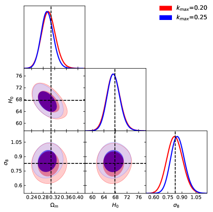
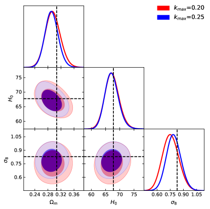
| high-z NGC | best-fit | mean |
|---|---|---|
| low-z NGC | best-fit | mean |
|---|---|---|
Now let us focus on Patchy mocks and consider the NGC mock datasets, which have bigger volumes. We fit the mean of 2048 mock power spectra with the covariance matrix of a single simulation box. This allows us to significantly reduce the statistical scatter among different realizations. For the analysis we assumed the same base CDM priors as the ones discussed above (see Tab. 3), along with the Gaussian prior . Note that we excluded the neutrino masses from the fit as the simulations were run for massless neutrinos. The multipoles of the mock catalogs were produced assuming a fiducial cosmology with , which is different from the true value used in the simulations. This is designed to introduce an additional anisotropy to be constrained through the AP effect.
We focused on four different choices of . Similarly to the case of LasDamas, our analysis suggests that at the systematic error becomes comparable to the statistical one, whereas at our model has too much freedom, and thus requires more narrow priors on the nuisance parameters in order to reduce the eventual errorbars. Given these reasons, we focus on in what follows. The posterior distribution obtained with our MCMC analysis is displayed in Fig. 10. The marginalized limits for the cosmological and bias parameters obtained in our mock catalog analysis for (which is used in our baseline analysis) are displayed in Table. 9.
One observes that for the best-fit and mean values of the inferred cosmological parameters are within from the true values, but some shifts w.r.t the true value are clearly visible. There are two sources of these shifts. First, there is a parameter projection effect, which can drive the mean values away from the best-fit along degeneracy directions. Put simply, these effects reflect that fact that the statistical error of the data is not good enough to break certain degeneracies among model parameters. We stress that this effect is somewhat different from the so-called prior volume effect. This effect takes place if the constraints on some parameters are prior-dominated, so that the mean values shift in certain directions allowed by the priors.
To study the projection effect we have run the same analysis with the survey volume of the mock covariances increased by a factor of 9. Just like in the LasDamas case, we have found the inferred means of and to be much closer to the true values, but still offset at the level of the new variance, which is reduced by a factor of compared to the actual BOSS volume. Another test was described in Section 5, where we analyzed mock datavectors generated with our theoretical model. Although the best-fit parameters obtained with our MCMC scans coincide with the input values, the means of some parameters (e.g. and ) were noticeably shifted. This suggests that the parameter projection effects are inevitable for the BOSS covariance, but can be reduced in future surveys with bigger volumes.
The second effect responsible for the shifts is a real systematic error related to higher-order corrections omitted in our theoretical model. We have found that our theoretical model can correctly recover the true cosmology of the mock data at even for survey volumes times bigger than the actual BOSS survey. However, it gives a biased estimate of if we go to higher ’s. This shift reaches at , which is still marginally smaller than our final statistical error on this parameter obtained by combining all the BOSS data samples. The systematic shifts observed in the estimated and are negligible (see the discussion above). Given these reasons, we decided to stick to because in this case the total marginalized error (statistical + systematic, added in quadratures) on the cosmological parameters is smaller than the similar error at , which is dominated by the statistical component.
Note that once we inflate the error to match the actual BOSS volume, the systematic error couples with volume effects, which shift the inferred value of instead of along the degeneracy direction between them. This correlation explains why the shifts of are negligible in Fig. 10, but become a leading systematic effect once we increase the survey volume in the covariance for the mock catalogs. The observed picture is, essentially, the same at for both redshift bins of the BOSS data.
All in all, we believe that the choice of represents a good balance between systematic and statistical errors. We emphasize that the 1d marginalized limits presented in this paper should not be over-interpreted beyond the level of uncertainty related to the inaccuracies of the theoretical modeling and parameter projection effects. Our tests on LasDamas mocks with higher volumes suggest that the shifts in the full parameter space (before marginalization) are actually much smaller than for the BOSS covariance.
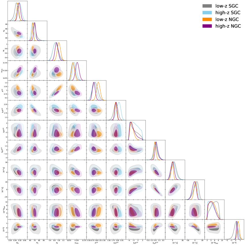
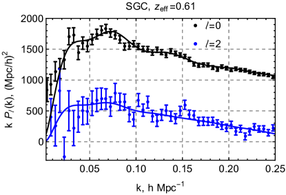
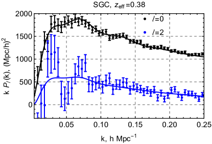
| high-z NGC | best-fit | mean |
|---|---|---|
| low-z NGC | best-fit | mean |
|---|---|---|
| high-z SGC | best-fit | mean |
|---|---|---|
| low-z SGC | best-fit | mean |
|---|---|---|
Appendix C Supplementary Material
In this Appendix we present some additional material. It includes full parameter constrain tables and corner plots for the baseline analysis, along with the results of the extended analyses that waived priors on the primordial power spectrum tilt and the neutrino mass. Finally, we show that are constraints are not sensitive to the data on very large scales, which are susceptible to systematics.
C.1 Full Triangle Plot and Constraint Tables
Let us present some additional material related to the baseline analysis with the Planck prior on . The results for the BBN priors are the same. The full triangle plot for four non-overlapping BOSS data chunks can be found in Fig. 11. We do not show the contours for and as they are prior-dominated. The corresponding 1d marginalized limits can be found in Table 10. For completeness, we also show the spectra for the SGC datasets along with the best-fit theoretical curves in Fig. 12. Similar plots for the NGC data were shown in Fig. 1.
Note that the reduced is a very inaccurate metric for the goodness of fit. First, it does not include the covariance between different -bins. Second, the naive reduced does not take into account that the cosmological constraints are always driven by the biggest wavenumbers used in the analysis. This is important to keep in mind when interpreting our results. Indeed, some of the values quoted in Table 10 (e.g. for the high-z SGC sample) are noticeably bigger than unity, which naively implies a bad fit. However, if we compute the reduced for the same parameters but using, e.g. /Mpc instead of /Mpc employed in our analysis, we find different numbers: , , , for the high-z NGC, low-z NGC, high-z SGC, and low-z SGC samples, respectively. Note a significant improvement for the high-z datasamples.
Note that the choice of within some reasonable range has a very mild effect on the parameter estimates (less than 1). This illustrates that the values quoted in Table 10 only give a very rough idea on the quality of the fit and hence should be taken with a grain of salt.
| best-fit | mean | |
|---|---|---|
| best-fit | mean | |
|---|---|---|
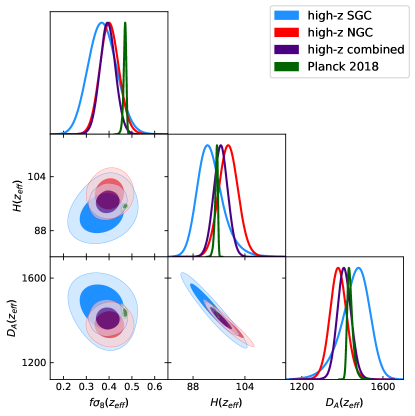
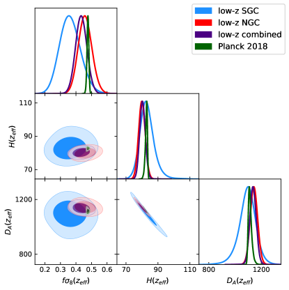
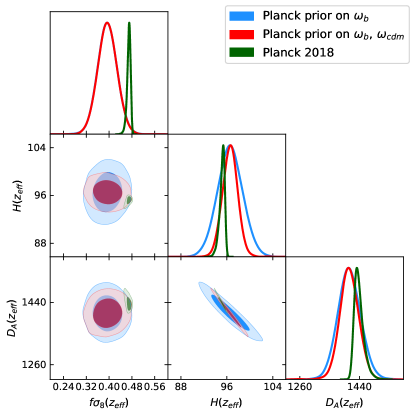
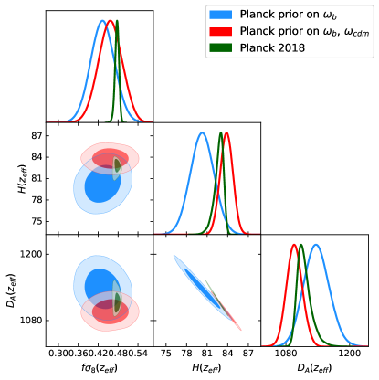
| high-z | best-fit | mean |
|---|---|---|
| low-z | best-fit | mean |
|---|---|---|
| high-z | best-fit | mean |
|---|---|---|
| low-z | best-fit | mean |
|---|---|---|
It is instructive to convert our results into the triplet at commonly used in the large-scale structure literature. We focus on the results obtained with the Planck prior on . The corresponding 2d posterior distribution projections are displayed in Fig. 13 (upper panels), 1d marginalized limits are given in Table. 12. For comparison, in Table. 11 we quote the limits extracted from the Planck MCMC chains run for CDM with a free neutrino mass. Overall, we see that the BOSS distance information is superseded by Planck, which gives much better constraints on and . One can notice a significant correlation between and in the corresponding panels. This degeneracy direction simply reflects the fact that in CDM these two quantities are related by definition, see Eq. (5.2), such that the product is nearly constant. We stress that the constraints on the distance parameters shown in Table. 12 do not use the Planck prior on .
C.2 Full Likelihood including the Power Spectrum Tilt
| BBN | best-fit | mean |
|---|---|---|
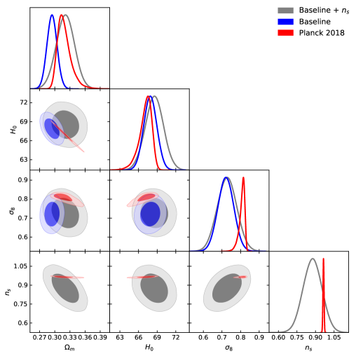
Our baseline analysis was performed for the fixed power spectrum tilt . In this Appendix we present the results of varying the full power spectrum likelihood. As in the baseline analysis, we keep the BBN prior on (3.23) and the prior on the neutrino masses (3.20), but do not assume any prior on whatsoever (i.e. we use a plat prior in the range ()). The results are displayed in Table 14 and in Fig. 14.
One observes that including to the fit notably worsens the precision of the measurement. This is to be expected as both these parameters are extracted from the power spectrum slope. The correlation between and backfires on the posterior distribution for , which shifts to a higher value almost by 1 w.r.t. our baseline analysis (with fixed ). In turn, pulls up and somewhat widens its marginalized posterior. Overall, the shift in is not very significant (). Note that the independent measurement of is consistent within 1 with the Planck CMB result.
C.3 Effect of Neutrino Masses
| low-z NGC, Baseline + | best-fit | mean |
|---|---|---|
| ( CL) | ||
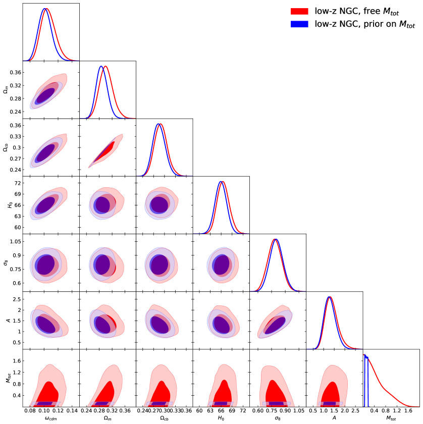
In this Appendix we present results of our analysis of the low-z NGC datasample without informative priors on the neutrino mass . Other than that, our methodology and priors are the same as in the baseline analysis. In particular, we assume the BBN prior on and fix to the Planck best-fit value. The results are presented in Table 15 and in Fig. 15.
The first relevant observation is that our constraints on and are almost insensitive to the neutrino mass. This must be contrasted with the Planck constraints on these parameters [44], which depend strongly on the neutrino masses. The second observation is that is, obviously, correlated with the neutrino mass and in this sense cannot be treated as an independent parameter. However, our limit on the late-time cold dark matter and baryon density fraction is almost the same in our baseline analysis and in the analysis with totally free . Thus, the measurements of from the BOSS data are quite robust w.r.t. the priors on the neutrino mass.
Overall, we conclude that BOSS alone are not very sensitive to the neutrino mass, and even very large around 1 eV is allowed. These values are already excluded by other cosmological probes, e.g. by the Ly-forest data alone (which sets a limit eV [49]), as well as by the particle physics laboratory experiments like KATRIN [102].
C.4 Effect of Large Scales
The BOSS spectra feature some spurious excess of power on scales Mpc-1. In Fig. 16 we show the results obtained from two analyses of the low-z NGC data: using all the -bins and having imposed the cut Mpc-1. The marginalized posteriors for and are identical to the ones obtained in our baseline analysis, whereas the mean value of is shifted upwards by when imposing the cut. Clearly, the signal is dominated by wavenumbers Mpc-1.
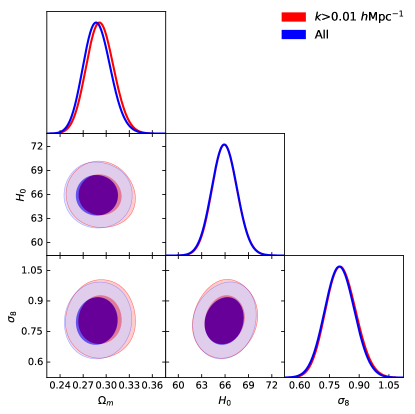
Appendix D Scaling Parameter Analysis
In this Section we give some details on our analysis in which we followed the standard parameterization and parameter estimation routine adopted in the previous BOSS FS analyses. We try to reproduce the analyses performed in Refs. [6, 5] as close as we could without a drastic modification of our pipeline. Our -analysis performed in this paper is only meant to capture some main qualitative features of the standard pipeline. It is not aimed at accurately reproducing the previous results.
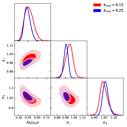
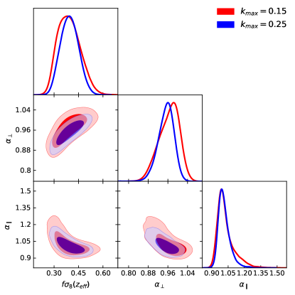
| high-z | best-fit | mean |
|---|---|---|
| low-z | best-fit | mean |
|---|---|---|
To match the standard methodology we modified our theoretical model to agree with the one used in the previous analyses. Specifically, we use
| (D.1) |
and do not introduce any RSD counterterms. The fingers-of-God effect is then described by only one parameter - the velocity dispersion . We have computed the theoretical power spectra for a fiducial cosmology with
| (D.2) |
which matches the parameters used in the most recent BOSS FS analysis [6]. We account for the AP effect by means of the scaling parameters , defined as
| (D.3) |
Overall, the cosmology-dependence of this model is parameterized by and . The non-linear bias and redshift-space distortion effects are parameterized by coefficients , , and the velocity dispersion . We fix the tidal bias to the value suggested by the coevolution model [16],
| (D.4) |
We use the same priors on the bias parameters as in our main analysis, except for , which is allowed to vary in the range [Mpc/]3. This is done in order to agree with the analysis of Ref. [6], which finds preferred values of the shot noise to be negative.
We studied two different choices of : and . The results of these analyses are shown in Fig. 17, where we display the marginalized posterior contours for low-z (left panel) and high-z (right panel) NGC samples. The 1d marginalized limits are presented in Table 16. One clearly sees that the inferred distance parameters become shifted w.r.t. the fiducial values at /Mpc. Moreover, the inferred values of the are more than 1-away from the Planck mean values. The distance measurements obtained with our -parametrization should be compared with the analysis of the DDE model, which found , to be very close to the Planck values. We believe that this difference is mainly produced by our choice of priors and the use of a different theoretical model.
References
- [1] LSST Science, LSST Project collaboration, P. A. Abell et al., LSST Science Book, Version 2.0, 0912.0201.
- [2] S. Dodelson, K. Heitmann, C. Hirata, K. Honscheid, A. Roodman, U. Seljak et al., Cosmic Visions Dark Energy: Science, 1604.07626.
- [3] O. Doré et al., Cosmology with the SPHEREX All-Sky Spectral Survey, 1412.4872.
- [4] EUCLID collaboration, R. Laureijs et al., Euclid Definition Study Report, 1110.3193.
- [5] H. Gil-Marín et al., The clustering of galaxies in the SDSS-III Baryon Oscillation Spectroscopic Survey: RSD measurement from the LOS-dependent power spectrum of DR12 BOSS galaxies, Mon. Not. Roy. Astron. Soc. 460 (2016) 4188 [1509.06386].
- [6] BOSS collaboration, F. Beutler et al., The clustering of galaxies in the completed SDSS-III Baryon Oscillation Spectroscopic Survey: Anisotropic galaxy clustering in Fourier-space, Mon. Not. Roy. Astron. Soc. 466 (2017) 2242 [1607.03150].
- [7] BOSS collaboration, J. N. Grieb et al., The clustering of galaxies in the completed SDSS-III Baryon Oscillation Spectroscopic Survey: Cosmological implications of the Fourier space wedges of the final sample, Mon. Not. Roy. Astron. Soc. 467 (2017) 2085 [1607.03143].
- [8] BOSS collaboration, S. Satpathy et al., The clustering of galaxies in the completed SDSS-III Baryon Oscillation Spectroscopic Survey: On the measurement of growth rate using galaxy correlation functions, Mon. Not. Roy. Astron. Soc. 469 (2017) 1369 [1607.03148].
- [9] BOSS collaboration, A. G. Sanchez et al., The clustering of galaxies in the completed SDSS-III Baryon Oscillation Spectroscopic Survey: cosmological implications of the configuration-space clustering wedges, Mon. Not. Roy. Astron. Soc. 464 (2017) 1640 [1607.03147].
- [10] D. Baumann, A. Nicolis, L. Senatore and M. Zaldarriaga, Cosmological Non-Linearities as an Effective Fluid, JCAP 1207 (2012) 051 [1004.2488].
- [11] J. J. M. Carrasco, M. P. Hertzberg and L. Senatore, The Effective Field Theory of Cosmological Large Scale Structures, JHEP 09 (2012) 082 [1206.2926].
- [12] P. McDonald and A. Roy, Clustering of dark matter tracers: generalizing bias for the coming era of precision LSS, JCAP 0908 (2009) 020 [0902.0991].
- [13] V. Assassi, D. Baumann, D. Green and M. Zaldarriaga, Renormalized Halo Bias, JCAP 1408 (2014) 056 [1402.5916].
- [14] L. Senatore, Bias in the Effective Field Theory of Large Scale Structures, JCAP 1511 (2015) 007 [1406.7843].
- [15] M. Lewandowski, A. Perko and L. Senatore, Analytic Prediction of Baryonic Effects from the EFT of Large Scale Structures, JCAP 1505 (2015) 019 [1412.5049].
- [16] V. Desjacques, D. Jeong and F. Schmidt, Large-Scale Galaxy Bias, Phys. Rept. 733 (2018) 1 [1611.09787].
- [17] L. Senatore and M. Zaldarriaga, Redshift Space Distortions in the Effective Field Theory of Large Scale Structures, 1409.1225.
- [18] A. Perko, L. Senatore, E. Jennings and R. H. Wechsler, Biased Tracers in Redshift Space in the EFT of Large-Scale Structure, 1610.09321.
- [19] D. J. Eisenstein, H.-j. Seo and M. J. White, On the Robustness of the Acoustic Scale in the Low-Redshift Clustering of Matter, Astrophys. J. 664 (2007) 660 [astro-ph/0604361].
- [20] M. Crocce and R. Scoccimarro, Nonlinear Evolution of Baryon Acoustic Oscillations, Phys. Rev. D77 (2008) 023533 [0704.2783].
- [21] N. S. Sugiyama and D. N. Spergel, How does non-linear dynamics affect the baryon acoustic oscillation?, JCAP 1402 (2014) 042 [1306.6660].
- [22] F. Bernardeau, S. Colombi, E. Gaztanaga and R. Scoccimarro, Large scale structure of the universe and cosmological perturbation theory, Phys. Rept. 367 (2002) 1 [astro-ph/0112551].
- [23] Z. Vlah, M. White and A. Aviles, A Lagrangian effective field theory, JCAP 1509 (2015) 014 [1506.05264].
- [24] Z. Vlah, E. Castorina and M. White, The Gaussian streaming model and convolution Lagrangian effective field theory, JCAP 1612 (2016) 007 [1609.02908].
- [25] L. Senatore and M. Zaldarriaga, The IR-resummed Effective Field Theory of Large Scale Structures, JCAP 1502 (2015) 013 [1404.5954].
- [26] T. Baldauf, M. Mirbabayi, M. Simonović and M. Zaldarriaga, Equivalence Principle and the Baryon Acoustic Peak, Phys. Rev. D92 (2015) 043514 [1504.04366].
- [27] Z. Vlah, U. Seljak, M. Y. Chu and Y. Feng, Perturbation theory, effective field theory, and oscillations in the power spectrum, JCAP 1603 (2016) 057 [1509.02120].
- [28] D. Blas, M. Garny, M. M. Ivanov and S. Sibiryakov, Time-Sliced Perturbation Theory II: Baryon Acoustic Oscillations and Infrared Resummation, JCAP 1607 (2016) 028 [1605.02149].
- [29] L. Senatore and G. Trevisan, On the IR-Resummation in the EFTofLSS, JCAP 1805 (2018) 019 [1710.02178].
- [30] M. M. Ivanov and S. Sibiryakov, Infrared Resummation for Biased Tracers in Redshift Space, JCAP 1807 (2018) 053 [1804.05080].
- [31] M. Lewandowski and L. Senatore, An analytic implementation of the IR-resummation for the BAO peak, 1810.11855.
- [32] D. J. Eisenstein, H.-j. Seo, E. Sirko and D. Spergel, Improving Cosmological Distance Measurements by Reconstruction of the Baryon Acoustic Peak, Astrophys. J. 664 (2007) 675 [astro-ph/0604362].
- [33] N. Padmanabhan, M. White and J. D. Cohn, Reconstructing Baryon Oscillations: A Lagrangian Theory Perspective, Phys. Rev. D79 (2009) 063523 [0812.2905].
- [34] Y. Feng, U. Seljak and M. Zaldarriaga, Exploring the posterior surface of the large scale structure reconstruction, JCAP 1807 (2018) 043 [1804.09687].
- [35] F. Schmidt, F. Elsner, J. Jasche, N. M. Nguyen and G. Lavaux, A rigorous EFT-based forward model for large-scale structure, JCAP 1901 (2019) 042 [1808.02002].
- [36] F. Elsner, F. Schmidt, J. Jasche, G. Lavaux and N.-M. Nguyen, Cosmology Inference from Biased Tracers using the EFT-based Likelihood, 1906.07143.
- [37] C. Alcock and B. Paczynski, An evolution free test for non-zero cosmological constant, Nature 281 (1979) 358.
- [38] M. Schmittfull, Z. Vlah and P. McDonald, Fast large scale structure perturbation theory using one-dimensional fast Fourier transforms, Phys. Rev. D93 (2016) 103528 [1603.04405].
- [39] J. E. McEwen, X. Fang, C. M. Hirata and J. A. Blazek, FAST-PT: a novel algorithm to calculate convolution integrals in cosmological perturbation theory, JCAP 1609 (2016) 015 [1603.04826].
- [40] M. Schmittfull and Z. Vlah, FFT-PT: Reducing the two-loop large-scale structure power spectrum to low-dimensional radial integrals, Phys. Rev. D94 (2016) 103530 [1609.00349].
- [41] X. Fang, J. A. Blazek, J. E. McEwen and C. M. Hirata, FAST-PT II: an algorithm to calculate convolution integrals of general tensor quantities in cosmological perturbation theory, JCAP 1702 (2017) 030 [1609.05978].
- [42] M. Simonović, T. Baldauf, M. Zaldarriaga, J. J. Carrasco and J. A. Kollmeier, Cosmological perturbation theory using the FFTLog: formalism and connection to QFT loop integrals, JCAP 1804 (2018) 030 [1708.08130].
- [43] D. Blas, J. Lesgourgues and T. Tram, The Cosmic Linear Anisotropy Solving System (CLASS) II: Approximation schemes, JCAP 1107 (2011) 034 [1104.2933].
- [44] Planck collaboration, N. Aghanim et al., Planck 2018 results. VI. Cosmological parameters, 1807.06209.
- [45] B. Audren, J. Lesgourgues, K. Benabed and S. Prunet, Conservative Constraints on Early Cosmology: an illustration of the Monte Python cosmological parameter inference code, JCAP 1302 (2013) 001 [1210.7183].
- [46] B. Audren, Separate Constraints on Early and Late Cosmology, Mon. Not. Roy. Astron. Soc. 444 (2014) 827 [1312.5696].
- [47] Particle Data Group collaboration, M. Tanabashi et al., Review of Particle Physics, Phys. Rev. D98 (2018) 030001.
- [48] K. N. Abazajian et al., Light Sterile Neutrinos: A White Paper, 1204.5379.
- [49] N. Palanque-Delabrouille, C. Yèche, N. Schöneberg, J. Lesgourgues, M. Walther, S. Chabanier et al., Hints, neutrino bounds and WDM constraints from SDSS DR14 Lyman- and Planck full-survey data, 1911.09073.
- [50] DES collaboration, T. M. C. Abbott et al., Dark Energy Survey year 1 results: Cosmological constraints from galaxy clustering and weak lensing, Phys. Rev. D98 (2018) 043526 [1708.01530].
- [51] H. Gil-Marín, J. Noreña, L. Verde, W. J. Percival, C. Wagner, M. Manera et al., The power spectrum and bispectrum of SDSS DR11 BOSS galaxies – I. Bias and gravity, Mon. Not. Roy. Astron. Soc. 451 (2015) 539 [1407.5668].
- [52] H. Gil-Marín, W. J. Percival, L. Verde, J. R. Brownstein, C.-H. Chuang, F.-S. Kitaura et al., The clustering of galaxies in the SDSS-III Baryon Oscillation Spectroscopic Survey: RSD measurement from the power spectrum and bispectrum of the DR12 BOSS galaxies, Mon. Not. Roy. Astron. Soc. 465 (2017) 1757 [1606.00439].
- [53] J. Lesgourgues and S. Pastor, Massive neutrinos and cosmology, Phys. Rept. 429 (2006) 307 [astro-ph/0603494].
- [54] N. Kaiser, Clustering in real space and in redshift space, Mon. Not. Roy. Astron. Soc. 227 (1987) 1.
- [55] L. F. de la Bella, D. Regan, D. Seery and D. Parkinson, Impact of bias and redshift-space modelling for the halo power spectrum: Testing the effective field theory of large-scale structure, 1805.12394.
- [56] A. Chudaykin and M. M. Ivanov, Measuring neutrino masses with large-scale structure: Euclid forecast with controlled theoretical error, 1907.06666.
- [57] M. Mirbabayi, F. Schmidt and M. Zaldarriaga, Biased Tracers and Time Evolution, JCAP 1507 (2015) 030 [1412.5169].
- [58] J. C. Jackson, Fingers of God: A critique of Rees’ theory of primoridal gravitational radiation, Mon. Not. Roy. Astron. Soc. 156 (1972) 1P [0810.3908].
- [59] N. Hand, U. Seljak, F. Beutler and Z. Vlah, Extending the modeling of the anisotropic galaxy power spectrum to , JCAP 1710 (2017) 009 [1706.02362].
- [60] M. Schmittfull, M. Simonović, V. Assassi and M. Zaldarriaga, Modeling Biased Tracers at the Field Level, 1811.10640.
- [61] T. Baldauf, M. Mirbabayi, M. Simonović and M. Zaldarriaga, LSS constraints with controlled theoretical uncertainties, 1602.00674.
- [62] BOSS collaboration, S. Alam et al., The clustering of galaxies in the completed SDSS-III Baryon Oscillation Spectroscopic Survey: cosmological analysis of the DR12 galaxy sample, Mon. Not. Roy. Astron. Soc. 470 (2017) 2617 [1607.03155].
- [63] A. J. S. Hamilton, Uncorrelated modes of the nonlinear power spectrum, Mon. Not. Roy. Astron. Soc. 312 (2000) 257 [astro-ph/9905191].
- [64] F.-S. Kitaura et al., The clustering of galaxies in the SDSS-III Baryon Oscillation Spectroscopic Survey: mock galaxy catalogues for the BOSS Final Data Release, Mon. Not. Roy. Astron. Soc. 456 (2016) 4156 [1509.06400].
- [65] J. Hartlap, P. Simon and P. Schneider, Why your model parameter confidences might be too optimistic: Unbiased estimation of the inverse covariance matrix, Astron. Astrophys. (2006) [astro-ph/0608064].
- [66] W. J. Percival et al., The Clustering of Galaxies in the SDSS-III Baryon Oscillation Spectroscopic Survey: Including covariance matrix errors, Mon. Not. Roy. Astron. Soc. 439 (2014) 2531 [1312.4841].
- [67] Y. Li, S. Singh, B. Yu, Y. Feng and U. Seljak, Disconnected Covariance of 2-point Functions in Large-Scale Structure, JCAP 1901 (2019) 016 [1811.05714].
- [68] E. Aver, K. A. Olive and E. D. Skillman, The effects of He I 10830 on helium abundance determinations, JCAP 1507 (2015) 011 [1503.08146].
- [69] R. J. Cooke, M. Pettini and C. C. Steidel, One Percent Determination of the Primordial Deuterium Abundance, Astrophys. J. 855 (2018) 102 [1710.11129].
- [70] N. Schöneberg, J. Lesgourgues and D. C. Hooper, The BAO+BBN take on the Hubble tension, 1907.11594.
- [71] E. G. Adelberger et al., Solar fusion cross sections II: the pp chain and CNO cycles, Rev. Mod. Phys. 83 (2011) 195 [1004.2318].
- [72] O. Pisanti, A. Cirillo, S. Esposito, F. Iocco, G. Mangano, G. Miele et al., PArthENoPE: Public Algorithm Evaluating the Nucleosynthesis of Primordial Elements, Comput. Phys. Commun. 178 (2008) 956 [0705.0290].
- [73] L. E. Marcucci, G. Mangano, A. Kievsky and M. Viviani, Implication of the proton-deuteron radiative capture for Big Bang Nucleosynthesis, Phys. Rev. Lett. 116 (2016) 102501 [1510.07877].
- [74] C. Pitrou, A. Coc, J.-P. Uzan and E. Vangioni, Precision big bang nucleosynthesis with improved Helium-4 predictions, Phys. Rept. 754 (2018) 1 [1801.08023].
- [75] E. Aubourg et al., Cosmological implications of baryon acoustic oscillation measurements, Phys. Rev. D92 (2015) 123516 [1411.1074].
- [76] P. Lemos, E. Lee, G. Efstathiou and S. Gratton, Model independent reconstruction using the cosmic inverse distance ladder, Mon. Not. Roy. Astron. Soc. 483 (2019) 4803 [1806.06781].
- [77] T. Lazeyras, C. Wagner, T. Baldauf and F. Schmidt, Precision measurement of the local bias of dark matter halos, JCAP 1602 (2016) 018 [1511.01096].
- [78] S. A. Rodríguez-Torres et al., The clustering of galaxies in the SDSS-III Baryon Oscillation Spectroscopic Survey: modelling the clustering and halo occupation distribution of BOSS CMASS galaxies in the Final Data Release, Mon. Not. Roy. Astron. Soc. 460 (2016) 1173 [1509.06404].
- [79] T. Baldauf, U. Seljak, R. E. Smith, N. Hamaus and V. Desjacques, Halo stochasticity from exclusion and nonlinear clustering, Phys. Rev. D88 (2013) 083507 [1305.2917].
- [80] C. Hahn, R. Scoccimarro, M. R. Blanton, J. L. Tinker and S. A. Rodríguez-Torres, The effect of fibre collisions on the galaxy power spectrum multipoles, Mon. Not. Roy. Astron. Soc. 467 (2017) 1940 [1609.01714].
- [81] T. Brinckmann and J. Lesgourgues, MontePython 3: boosted MCMC sampler and other features, 1804.07261.
- [82] A. Lewis and S. Bridle, Cosmological parameters from CMB and other data: A Monte Carlo approach, Phys. Rev. D66 (2002) 103511 [astro-ph/0205436].
- [83] A. Lewis, Efficient sampling of fast and slow cosmological parameters, Phys. Rev. D87 (2013) 103529 [1304.4473].
- [84] A. Gelman and D. B. Rubin, Inference from Iterative Simulation Using Multiple Sequences, Statist. Sci. 7 (1992) 457.
- [85] S. P. Brooks and A. Gelman, General Methods for Monitoring Convergence of Iterative Simulations, J. Comp. Graph. Stat. 7 (1997) 434.
- [86] BOSS collaboration, F. Beutler et al., The clustering of galaxies in the SDSS-III Baryon Oscillation Spectroscopic Survey: Testing gravity with redshift-space distortions using the power spectrum multipoles, Mon. Not. Roy. Astron. Soc. 443 (2014) 1065 [1312.4611].
- [87] 2dFGRS Team collaboration, W. J. Percival et al., Parameter constraints for flat cosmologies from CMB and 2dFGRS power spectra, Mon. Not. Roy. Astron. Soc. 337 (2002) 1068 [astro-ph/0206256].
- [88] A. Cuceu, J. Farr, P. Lemos and A. Font-Ribera, Baryon Acoustic Oscillations and the Hubble Constant: Past, Present and Future, 1906.11628.
- [89] A. G. Riess, S. Casertano, W. Yuan, L. M. Macri and D. Scolnic, Large Magellanic Cloud Cepheid Standards Provide a 1% Foundation for the Determination of the Hubble Constant and Stronger Evidence for Physics beyond CDM, Astrophys. J. 876 (2019) 85 [1903.07603].
- [90] K. C. Wong et al., H0LiCOW XIII. A 2.4% measurement of from lensed quasars: tension between early and late-Universe probes, 1907.04869.
- [91] Y. Kobayashi, T. Nishimichi, M. Takada and R. Takahashi, Cosmological information content in redshift-space power spectrum of SDSS-like galaxies in the quasi-nonlinear regime up to Mpc-1, 1907.08515.
- [92] SDSS collaboration, M. Tegmark et al., Cosmological Constraints from the SDSS Luminous Red Galaxies, Phys. Rev. D74 (2006) 123507 [astro-ph/0608632].
- [93] W. J. Percival et al., The shape of the SDSS DR5 galaxy power spectrum, Astrophys. J. 657 (2007) 645 [astro-ph/0608636].
- [94] B. A. Reid et al., Cosmological Constraints from the Clustering of the Sloan Digital Sky Survey DR7 Luminous Red Galaxies, Mon. Not. Roy. Astron. Soc. 404 (2010) 60 [0907.1659].
- [95] J. Hamann, S. Hannestad, J. Lesgourgues, C. Rampf and Y. Y. Y. Wong, Cosmological parameters from large scale structure - geometric versus shape information, JCAP 1007 (2010) 022 [1003.3999].
- [96] BOSS collaboration, F. Beutler et al., The clustering of galaxies in the completed SDSS-III Baryon Oscillation Spectroscopic Survey: baryon acoustic oscillations in the Fourier space, Mon. Not. Roy. Astron. Soc. 464 (2017) 3409 [1607.03149].
- [97] M. Ata et al., The clustering of the SDSS-IV extended Baryon Oscillation Spectroscopic Survey DR14 quasar sample: first measurement of baryon acoustic oscillations between redshift 0.8 and 2.2, Mon. Not. Roy. Astron. Soc. 473 (2018) 4773 [1705.06373].
- [98] H. Gil-Marín et al., The clustering of the SDSS-IV extended Baryon Oscillation Spectroscopic Survey DR14 quasar sample: structure growth rate measurement from the anisotropic quasar power spectrum in the redshift range , Mon. Not. Roy. Astron. Soc. 477 (2018) 1604 [1801.02689].
- [99] G. D’Amico, J. Gleyzes, N. Kokron, D. Markovic, L. Senatore, P. Zhang et al., The Cosmological Analysis of the SDSS/BOSS data from the Effective Field Theory of Large-Scale Structure, 1909.05271.
- [100] D. Blas, M. Garny, M. M. Ivanov and S. Sibiryakov, Time-Sliced Perturbation Theory for Large Scale Structure I: General Formalism, JCAP 1607 (2016) 052 [1512.05807].
- [101] C. McBride, A. Berlind, R. Scoccimarro, R. Wechsler, M. Busha, J. Gardner et al., LasDamas Mock Galaxy Catalogs for SDSS, in American Astronomical Society Meeting Abstracts #213, vol. 213 of American Astronomical Society Meeting Abstracts, p. 425.06, Jan, 2009.
- [102] KATRIN collaboration, M. Aker et al., Improved Upper Limit on the Neutrino Mass from a Direct Kinematic Method by KATRIN, Phys. Rev. Lett. 123 (2019) 221802 [1909.06048].