Plateau Proposal Distributions for Adaptive Component-wise Multiple-Try Metropolis

Abstract

Markov chain Monte Carlo (MCMC) methods are sampling methods that have become a commonly used tool in statistics, for example to perform Monte Carlo integration. As a consequence of the increase in computational power, many variations of MCMC methods exist for generating samples from arbitrary, possibly complex, target distributions. The performance of an MCMC method is predominately governed by the choice of the so-called proposal distribution used. In this paper, we introduce a new type of proposal distribution for the use in MCMC methods that operates component-wise and with multiple trials per iteration. Specifically, the novel class of proposal distributions, called Plateau distributions, do not overlap, thus ensuring that the multiple trials are drawn from different regions of the state space. Furthermore, the Plateau proposal distributions allow for a bespoke adaptation procedure that lends itself to a Markov chain with efficient problem dependent state space exploration and improved burn-in properties. Simulation studies show that our novel MCMC algorithm outperforms competitors when sampling from distributions with a complex shape, highly correlated components or multiple modes.

1 Introduction

Markov chain Monte Carlo (MCMC) methods are essentially used to perform Monte Carlo integration, which has become a standard statistical tool. Specifically, MCMC methods produce samples from a target distribution $\pi$ by using an ergodic Markov chain with stationary distribution $\pi$. Typically, MCMC methods are used when it is difficult to sample from the target distribution directly, e.g. when the normalisation constant is unknown. There are many ways to construct this Markov chain which have lead to many variations of MCMC methods; see, e.g., Brooks et al., (2011).

The classic MCMC method is the Metropolis-Hastings algorithm (Metropolis et al.,, 1953). At each iteration, the Metropolis-Hastings algorithm is designed to update the entire current state (i.e. all components of the random vector generated at the previous iteration) at once. However, updating individual components, or subsets of components, is possible. Indeed, this type of component-wise updating was initially proposed in Metropolis et al., (1953), but did not receive much attention at first. In this paper, we focus on updating individual components. Using individual component updates is a way of sampling from the (lower dimensional) conditional distributions of the target, provided the conditional distributions are known. However, this is typically not the case in practise. An approach to remedy this is to model the conditional distributions. However, using parametric models leads to an inflexible approximation whereas non-parametric models do not scale well with the number of dimensions. For these reasons, we focus our attention on independent component-wise updates.

Another variant of MCMC sampling is the multiple-try method (Jun S. Liu,, 2000) where several proposals or trials are suggested at each iteration, as opposed to a single proposal. The motivation behind the multiple-try method is that more of the space is explored at the expense of an increased computational cost (i.e. proposal generation and evaluation of acceptance criterion). In fact, the multiple-try approach is known to offer great flexibility in terms of designing MCMC methods that satisfy detailed balance. As a consequence, several variations exist in the literature; see also the discussion in Martino and Read, (2013).

Recently, in Yang et al., (2019) the authors introduce a component-wise, multiple-try MCMC method with Gaussian proposals for each trial, where each univariate proposal has a different variance. In this work, we introduce a new class of proposal distributions for use in a component-wise, multiple-try MCMC method. These proposals, called Plateau distributions, do not overlap to exploit the multiple-try nature of the method. Indeed, by using proposals that do not overlap for each trial, the Markov chain is forced to explore different parts of the state-space. Conversely, using proposals that overlap, e.g. Gaussians with different variances, can lead to an inefficient algorithm, as the trials tend to be from a similar region of the state-space.

Using Plateau distributions for the proposal distributions leads to better exploration of the space over standard Gaussian proposals. The idea is intuitive, easy to implement and leads to good results, in the sense of exploring the state space. Moreover, using the Plateau proposals leads to a reversible Markov chain with the target distribution as its invariant distribution e.g. see Yang et al., (2019).

As is common for most proposals used in MCMC methods, the Plateau distributions depend on parameters that need to be selected with respect to the target distribution to obtain an effective MCMC algorithm. Adaptation of MCMC methods typically entails tuning the parameter(s) of a class of proposal distributions, e.g. the variance parameter in a Normal distribution, in order to improve the convergence properties of the Markov chain. For instance, in Haario et al., (2001), a Gaussian proposal distribution is used whose variance (or covariance) is adapted using the previously generated states of the Markov chain.

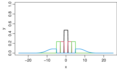
(a)

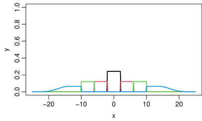
(b)

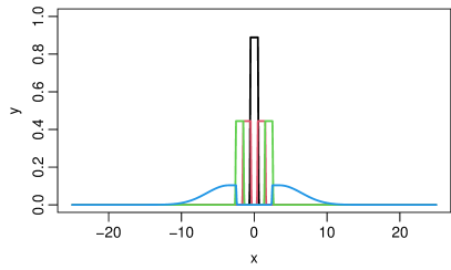
(c)

Figure 1: Illustration of $4$ Plateau proposal distributions (probability density functions) represented by the different colours and the adaptation procedure. The initial Plateau distributions are presented in (a); If the outermost (blue) proposals are selected frequently, the proposals are adapted to (b); If innermost (black) proposals are selected frequently, the proposals are adapted to (c).

In this work we propose an adaptation procedure that is designed for use with the non-overlapping multiple-try Plateau proposals. The Plateau proposals together with the associated adaptation procedure are exemplified in Fig. 1. Suppose the MCMC algorithm is initiated with multiple-try proposals whose distributions are presented by the different coloured lines in Fig. 1a. These proposals operate independently on each (univariate) component in the target space. As the Markov chain evolves, the number of times each Plateau’s proposed candidate state is selected is recorded. If the innermost or outermost Plateaus are overly selected, then the set of Plateau proposals are re-organised as depicted in Figs. 1b and 1b. More precisely, if the innermost (black) proposal is overly selected, then one halves the width of each plateau and shifts the set of proposals to remove the gaps. A similar procedure is conducted if the outermost (blue) proposals is overly selected by doubling the width of the plateaus. This procedure appropriately scales the set of Plateau proposals to the target distribution. Notice that this intuitive adaptation procedure makes explicit use of the non-overlapping feature of the Plateau proposals. Specifically, if a sample is selected from a particular Plateau distribution, then that sample could not have been obtained by sampling from any other Plateau distribution since their supports do not overlap. Therefore, counting the number of times each Plateau is selected gives a clear and direct indication as to how to update the Plateaus to match the shape of the target. This indication is not so clear when using proposals that overlap. The advantages of using non-overlapping proposals, as opposed to overlapping proposals, is explored in Section 5. The mathematical definition of the Plateau proposals and the pseudocode for the adaptation procedure are presented later in Sections 3 and 4 respectively.

The works in Giordani and Kohn, (2010) and Craiu and Lemieux, (2007) share a similar objective with our proposed work, namely: draw samples that are far apart from each other to facilitate an effective exploration of the state-space. For example, in Giordani and Kohn, (2010) the authors introduce an independent (i.e., component-wise), yet single-try, Metropolis–Hastings method using a normal mixture distribution as proposal. To achieve a more structured state space exploration, the mixture distribution is adapted, based an appropriate $k$-means clustering of chain’s visited states. In Craiu and Lemieux, (2007) an improved state space exploration is achieved by combining variance reduction techniques with multiple trials. Specifically, it involves drawing multiple trails from a single, well-chosen proposal distribution that is based on, e.g., Latin Hypercube sampling. The performance of these approaches depends on a well-chosen transformation. Conversely, the approach introduced in this work does not require such a transformation, as the Plateau proposals reside in the state space. Further, our adaptation procedure automates the tuning of the Plateau proposals parameters and does not require additional clustering (i.e., optimisation) algorithms to be performed.

To summarise, the goal of this work is to propose a new MCMC algorithm along with an adaptation procedure, which is simple to implement, intuitive and can by used without using explicit derivative information (e.g. Hamiltonian Monte Carlo Neal et al., (2011)) or conditional distributions (e.g. Gibbs sampling Casella and George, (1992)) of the target. Therefore a general-purpose MCMC algorithm is required. To this end, we introduce Plateau proposals as a general class of proposal distributions for use in a component-wise multiple-try MCMC methods. Specifically, the combination of non-overlapping characteristic of Plateau proposals with the multiple-try approach lends itself to a bespoke adaptation procedure that leads to good results for a variety of target distributions. This is achieved by improved state space exploration and favourable burn-in properties.

The remainder of this is organised as follows. In Section 2.1 a generic component-wise multiple-try algorithm is presented. The novel class of Plateau proposals is introduced and discussed in Section 3. In Section 4 we discuss how to adaptively select the parameter of the Plateau proposals and offer a detailed algorithmic description of the complete method. The performance of our new method is then compared with other MCMC methods in Section 6. Finally, a commentary on improvements and a summary are provided in Section 7.

2 Component-wise Update with Multiple Trials

Let $\pi$ be a probability density function, $\pi\colon\mathcal{X}\to\mathbb{R}^{+}$, where $\mathcal{X}\subseteq\mathbb{R}^{d}$. Our main interest is to sample from $\pi$; this is the target distribution. We assume that sampling directly from $\pi$ is difficult or impossible, for example because $\pi$ may only be known up to a multiplicative constant. In order to sample from $\pi$ we use MCMC methods. Specifically, given the current state $\boldsymbol{X}_{n}=\boldsymbol{x}\in\mathcal{X}$ of the Markov chain at iteration $n\in\mathbb{N}$, the Metropolis-Hastings algorithm, one of the simplest MCMC methods, proposes a candidate $\boldsymbol{Y}$ for the chain’s next state $\boldsymbol{X}_{n+1}$ by drawing a random variable from distribution with probability density function (PDF) $T(\boldsymbol{x},\cdot)\colon\mathcal{X}\to\mathbb{R}^{+}$ from which it is easier to sample from than from the target distribution. That is $\boldsymbol{Y}\sim T(\boldsymbol{x},\cdot)$, where $T(\boldsymbol{x},\cdot)$ is the conditional density given the current value $\boldsymbol{x}$ of, what is commonly known as, the proposal distribution. For example, the random-walk proposal Metropolis et al., (1953); Hastings, (1970) uses a multivariate normal distribution, which we will write as $T(\boldsymbol{x},\cdot)=\mathrm{N}(\boldsymbol{x},\sigma^{2}I)$ with $\sigma>0$ given and $I$ being the $d\times d$ identity matrix. Another example is $\mathrm{N}\bigl{(}\boldsymbol{x}+\tau\nabla\ln\bigl{(}\pi(\boldsymbol{x})\bigr{)},2\tau I)$ with $\tau>0$ fixed, which is the proposal used in the Metropolis-adjusted Langevin algorithm Roberts and Tweedie, (1996). The realisation of the Markov chain’s next state is then selected by means of an accept-reject procedure in a way such that the resulting Markov chain’s stationary distribution is $\pi$.

One of the main difficulties when using an MCMC method is the choice of the proposal distribution. In particular, the choice of the proposal may significantly affect the properties of the MCMC method, including the speed of convergence to equilibrium and mixing properties Rosenthal, (2011). Typically, the proposal distribution is selected from some family of well-known distributions, e.g., from the family of normal distributions. It is noteworthy that an optimal MCMC performance in high dimensions requires to select the “scale” of the proposal appropriately (e.g. see Roberts and Rosenthal,, 2001).

Instead of proposing a single multivariate candidate from $\boldsymbol{Y}\sim T(\boldsymbol{x},\cdot)$ by updating all components of the current state $\boldsymbol{X}_{n}=\boldsymbol{x}$ simultaneously via the (global) proposal distribution $T(\boldsymbol{x},\cdot)$, it is also possible to split the state space $\mathcal{X}$ into its individual components (or small groups of components) and propose candidates for each component (or group of components) independently. This local (or projected) approach is intuitive, computationally efficient, and reduces the problem of selecting a multidimensional proposal into lower dimensional proposals that are easier to handle. MCMC methods using these types of updates are called component-wise MCMC methods which may use a potentially different proposal distribution per component of the state (Gilks et al.,, 1995, Ch. 1). In this work we focus on one-dimensional, component-wise proposals. We emphasise, however, that the ideas that follow are not restricted to one-dimensional components and are general in fact.

Considering independent one-dimensional, component-wise proposals is equivalent to the proposal distribution $T(\boldsymbol{x},\cdot)$ given $\boldsymbol{x}=(x_{1},\dots,x_{d})\in\mathbb{R}^{d}$ being separable, in the sense that

$$T(\boldsymbol{x},\boldsymbol{y})\equiv T_{1}(x_{1},y_{1})\times\dots\times T_{d}(x_{d},y_{d})=\prod_{k=1}^{d}T_{k}(x_{k},y_{k})\;,$$ (1)

for any $\boldsymbol{y}=(y_{1},\dots,y_{d})\in\mathbb{R}^{d}$. Here, $T_{k}(x,\cdot)\colon\mathbb{R}\to\mathbb{R}^{+}$, $k=1,\dots,d$ with $x\in\mathbb{R}$, denotes the one-dimensional proposal density given $x$ used to draw the candidate for component $k$. That is, the proposed (global) candidate $\boldsymbol{Y}=(Y_{1},\dots,Y_{d})\in\mathbb{R}^{d}$ is obtained by sampling each $Y_{k}\sim T_{k}(x_{k},\cdot)$ mutually independent from any other $Y_{\ell}$. Notice that this one-dimensional, component-wise proposal step is identical to the standard MCMC method with $d=1$, and hence can be considered a natural extension to the multivariate case.

While the component-wise candidate proposal (1) is computationally efficient, by construction it does not account for correlations between the components. Consequently, the proposed candidates $\boldsymbol{Y}$ may not be good representatives of the target distribution $\pi$ (i.e. most candidates $\boldsymbol{Y}$ will be rejected, resulting in a very low acceptance rate), if $\pi$ has highly correlated components. Therefore these “uninformed” candidates may lead to a poor state space exploration and thus to a poor performance of the MCMC method. To remedy these defects, we will combine component-wise proposals with multiple trials for each component. Specifically, the multiple-try technique works by proposing many candidates from a proposal distribution, rather than just a single one, amongst which the “best” one is selected. Each trial may be proposed from a different proposal distribution. Thus, in combination with component-wise proposals, we (independently) generate $M$ possible candidates (i.e., $M$ trials) independently for each component $k=1,\dots,d$. Let $T_{j,k}(x,\cdot)\colon\mathbb{R}\to\mathbb{R}^{+}$, $j=1,\dots,M$, denote the proposal PDF of the $j$th trial for the $k$th component given $x_{k}=x$.

2.1 Generic Procedure of Component-wise Multiple-Try Metropolis

A generic component-wise multiple-try algorithm is now described – the full pseudo-code for generating $N$ samples from the target distribution $\pi$ is presented in Algorithm 1. Each MCMC iteration of the algorithm involves drawing multiple trials and then performing an acceptance-rejection step for each component sequentially.

We now describe the intuition behind the steps of the procedure. Suppose that the state of the chain at the beginning of the $n$th iteration is $\boldsymbol{x}=(x_{1},\dots,x_{d})$. For the first component (i.e., $k=1$), $M$ independent trials, $z_{1},\dots,z_{M}\in\mathbb{R}$, are drawn from $T_{j,1}(x_{1},\cdot)$. These trials are then weighted according to

$$w_{j,1}(z_{j},\boldsymbol{x})=\pi\bigl{(}(z_{j};\boldsymbol{x}_{[-1]})\bigr{)}T_{j,1}(x_{1},z_{j})\lambda_{j,1}(x_{1},z_{j})\;,$$

where $(z;\boldsymbol{x}_{[-i]})\in\mathbb{R}^{d}$ denotes the vector that is identical to $\boldsymbol{x}$ except for its $i$th component which is replaced by $z\in\mathbb{R}$, that is $(z;\boldsymbol{x}_{[-i]})=(x_{1},\dots,x_{i-1},z,x_{i+1},\dots,x_{d})$.

The functions $\lambda_{j,k}(x,y)$ with $x,y\in\mathbb{R}$ for any $k=1,\dots d$, are non-negative, symmetric functions in $x$ and $y$ which are selected by the user. Further it is required that $\lambda_{j,k}(x,y)>0$ whenever $T_{j,k}(x,y)>0$. Each trial $z_{j}$, $j=1,\dots,M$, has an associated weight $w_{j,1}(z_{j},\boldsymbol{x})$. A candidate for the first component of the chain’s next state is then randomly selected amongst all trials $z_{j}$ $(j=1,\dots,M)$ according to these weights. The selected candidate is then accepted or rejected. The remaining components $k=2,3,\dots,d$ of the chain’s state are updated in order in a similar fashion; Algorithm 1 illustrates a detailed pseudo-code of the corresponding MCMC method.

0:  number of trials $M$; number of MCMC realisations $N$; starting position $\boldsymbol{x}_{0}\in\mathbb{R}^{d}$; target distribution $\pi$ (possibly un-normalised); proposal distributions $T_{j,k}$

1:  Let $\boldsymbol{X}_{0}=\boldsymbol{x}_{0}=\boldsymbol{x}$.

2:  for $n=1,\dots,N$ do

3:     for $k=1,\dots,d$ do

4:        Propose $M$ trials: $z_{j}\sim T_{j,k}(x_{k},\cdot)$ for $j=1,\dots,M$.

5:        Compute the trial weights

$$w_{j,k}(z_{j},\boldsymbol{x})=\pi\bigl{(}(z_{j};\boldsymbol{x}_{[-k]})\bigr{)}T_{j,k}(x_{k},z_{j})\lambda_{j,k}(x_{k},z_{j})\;,\quad j=1,\dots,M.$$

6:        Draw $y\in\{z_{1},\dots,z_{M}\}$ randomly with probability proportional to $w_{1,k},\dots,w_{M,k}$.

7:        Draw $x_{j}^{\ast}\sim T_{j,k}(y,\cdot)$ for $j=1,\dots,M-1$ and let $x_{M}^{\ast}=x_{k}$.

8:        Let $\boldsymbol{y}=(y;\boldsymbol{x}_{[-k]})$ and compute

$$\alpha=\min\left\{1,\frac{w_{1,k}(z_{1},\boldsymbol{x})+\dots+w_{M,k}(z_{M},\boldsymbol{x})}{w_{1,k}(x^{\ast}_{1},\boldsymbol{y})+\dots+w_{M,k}(x^{\ast}_{M},\boldsymbol{y})}\right\}.$$

Draw $r\sim\text{Uniform}(0,1)$.

9:        if $r<\alpha$ then

10:           Accept $\boldsymbol{X}_{n}=\boldsymbol{y}=(y;\boldsymbol{x}_{[-k]})$ and set $\boldsymbol{x}=\boldsymbol{y}$.

11:        else

12:           $\boldsymbol{X}_{n}=\boldsymbol{x}$.

13:        end if

14:     end for

15:  end for

16:  return  $\boldsymbol{X}_{1},\dots,\boldsymbol{X}_{N}$

Algorithm 1 Generic Component-wise Multiple-Try Metropolis

Specifically, to propose a candidate for the $k$th component of the Markov chain’s next state in step 5 of Algorithm 1 each trial for the current $k$th component $x_{k}$ has an associated weight

$$w_{j,k}(z_{j},\boldsymbol{x})=\pi\bigl{(}(z_{j};\boldsymbol{x}_{[-k]})\bigr{)}T_{j,k}(x_{k},z_{j})\lambda_{j,k}(x_{k},z_{j}),\quad j=1,\dots,M.$$

As described above, a single trial is then randomly selected with probabilities proportional to $w_{j,k}$. There are a number of choices for $\lambda_{j,k}$ in the multiple-try literature Jun S. Liu, (2000), such as

$$\left(\frac{T_{j,k}(x,y)+T_{j,k}(y,x)}{2}\right)^{-1},\quad\left\{T_{j,k}(x,y)T_{j,k}(y,x)\right\}^{-\beta}\quad\text{and}\quad 1.$$

In work Yang et al., (2019) the authors suggest to use

$$\lambda_{j,k}(x,y)=T_{j,k}(x,y)\left\lVert y-x\right\rVert^{\alpha}\;,$$ (2)

where $\alpha=2.9$ was used following a simulation study focusing on large moves in the state spaces. Here we will also use $\lambda_{j,k}$ as in (2). However, in simulations, not reported here, we found that $\alpha=2.5$ performed best in terms of the mean squared error for a variety of target distributions. Consequently we use $\lambda_{j,k}$ with $\alpha=2.5$ for the remainder of the paper. We note that it is beyond the scope of this paper to propose a particular form for the class of functions $\lambda_{j,k}$ due to the problem dependent nature of this choice. Instead we advocate that users perform a trial run with a variety of $\lambda_{j,k}$ to determine which is best suit for their application and performance metric.

3 Non-Overlapping Proposal Distributions

In principle, any family of proposals $T_{j,k}$ can be used in Algorithm 1. However, a careful choice of the proposals can lead to a more efficient algorithm.

Recall that $T_{j,k}$ is the $j$th trial proposal distribution for the $k$th component. As mentioned earlier, the motivation of using multiple trials is to explore a larger region of the state space than is achieved by using a single proposal. Therefore, it would not be beneficial to use proposals that are similar. To illustrate this, suppose that for a fixed component $k$ we use the proposal distributions $T_{j,k}(x,\cdot)=\mathrm{N}(x,(j\sigma)^{2})$ for $j=1,\dots,M=5$ with known $\sigma>0$ and take $x=0$ without loss of generality. The probability density functions of these proposals of with $\sigma=1$ are presented in Figure 2.

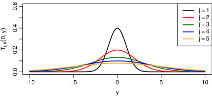
Figure 2: Probability density function of 5 Normal distributions with zero mean and standard deviations $j\sigma$ for $\sigma=1$, $j=1,\dots,5$.

As illustrated in Figure 2, these proposals are very similar. Indeed, $99$% of $T_{1,k}$’s density mass lies within the interval

$$\mathfrak{J}=\bigl{(}-\sigma\Phi^{-1}(0.995),\sigma\Phi^{-1}(0.995)\bigr{)}$$

centred around $x=0$, where $\Phi^{-1}$ is the inverse of the cumulative distribution function of a standard normal so that $\Phi^{-1}(0.995)\approx 2.6$. Suppose that we consider for the second proposal distribution $Y_{2,k}\sim T_{2,k}(0,\cdot)$, then $\mathbb{P}(Y_{2,k}\in\mathfrak{J})\approx 0.8$ for any $\sigma>0$. That is, draws from $T_{1,k}$ and $T_{2,k}$ will be located in the same region with high probability. Similar arguments hold for the wider Gaussian proposals. Thus draws from these Gaussian proposals will tend to be similar, thus leading to an inefficient use of the multiple-try technique. To avoid sampling similar proposals for each trial, we seek densities which do not overlap (or overlap to a small degree).

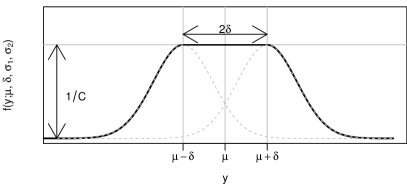
(a)

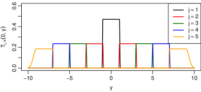
(b)

Figure 3: PDF of Plateau proposal distributions with $M=5$. The five different proposals each have a different colour.

Specifically, we advocate using proposals of the type illustrated in Figure 3b. That is, each trial for each component-wise proposal distribution combines uniform distributions with exponentially decaying tails. Notice, that this means that the amount of overlap between different proposals is controlled through how fast the tails decay. Specifically, we first introduce the PDF

$$f(y;\mu,\delta,\sigma_{1},\sigma_{2})=\frac{1}{C}\begin{cases}\exp\left\{-\frac{1}{2\sigma_{1}^{2}}\left[y-(\mu-\delta)\right]^{2}\right\}&\text{for }y<\mu-\delta\\ 1&\text{for }\mu-\delta\leq y\leq\delta+\mu\\ \exp\left\{-\frac{1}{2\sigma_{2}^{2}}\left[y-(\mu+\delta)\right]^{2}\right\}&\text{for }y>\mu+\delta\\ \end{cases}$$

where

$$C=\frac{\sqrt{2\pi\sigma_{1}^{2}}}{2}+\frac{\sqrt{2\pi\sigma_{2}^{2}}}{2}+2\delta$$

denotes the normalisation constant. This PDF is illustrated in Figure 3a. For each component $k$ with given value $x_{k}=x$, we then set the PDF of the each trial proposal as

$$T_{j,k}(x,y)=\begin{cases}f(y;x,\delta_{1},\sigma,\sigma)&j=1\\ \frac{1}{2}f(y;x-2(j-1)\delta_{1}-\delta,\delta,\sigma,\sigma)+\frac{1}{2}f(y;x+2(j-1)\delta_{1}+\delta,\delta,\sigma,\sigma)&j=2,\dots,M-1,\\ \frac{1}{2}f(y;x-2(M-1)\delta_{1}-\delta,\delta,\sigma_{0},\sigma)+\frac{1}{2}f(y;x+2(M-1)\delta_{1}+\delta,\delta,\sigma,\sigma_{1})&j=M\end{cases}$$

for some values of $\delta_{1},\delta,\sigma,\sigma_{0},\sigma_{1}>0$. The $M=5$ trial proposals shown in Figure 3b correspond to $\delta_{1}=\delta=1$, $\sigma=0.05$ and $\sigma_{0}=\sigma_{1}=0.5$. We shall refer to the proposals of this type as Plateau proposals given the shape of their PDFs. The $\delta_{1}$ parameter controls the width of the central Plateau centred at the current state $x$. The $\delta$ parameter is the width of the other Plateaus. The $\sigma$ value controls the decay of the tails either side of the inner Plateaus. The outer tails for the $M$th proposal are described by $\sigma_{0}$ and $\sigma_{1}$.

To compare with the earlier calculations for coverage probabilities for the Gaussian proposals; $99$% of the density of $T_{1,k}$ with $x=0$, $\delta=1$, and $\sigma=0.5$ lies in the interval $\mathfrak{J}=(-2.11,2.11)$. Suppose that $Y_{2,k}\sim T_{2,k}(0,\cdot)$, then $\mathbb{P}(Y_{2,k}\in\mathfrak{J})\approx 0.43$, which is reduced by almost a factor of two compared to the overlapping Gaussian proposal. Further, if $\sigma=0.25$ then $\mathbb{P}(Y_{2,k}\in\mathfrak{J})\approx 0.31$ and if $\sigma=0.05$ then $\mathbb{P}(Y_{2,k}\in\mathfrak{J})\approx 0.06$. Thus, the Plateau proposals overlap less than the Gaussian proposals example and further, the extent of the overlapping of the proposals is controlled by the values of $\sigma$, $\sigma_{1}$, and $\sigma_{2}$.

Note that each Plateau proposal distribution has a support on $\mathbb{R}$. This is to ensure that the support of the target distribution is included within the support of the proposals. In theory, this allows the Markov chain to explore the entire support of the target distribution. In a practical setting, however, by selecting the value of $\sigma$ appropriately, the tails of the distribution decay to zero very quickly, making the inner proposals effectively uniform distributions in view of numerical simulations. Therefore, in practice one could elect to sample from these distributions using direct draws from Uniform distributions to increase computation speed. However, in all the experiments performed in this paper, we sample from the exact Plateau proposal distributions defined above.

Note that the suggested Plateau proposals are very general; the choice of proposal parameters, $\delta$, $\delta_{1}$, $\sigma$, $\sigma_{0}$ and $\sigma_{1}$, allow for diverse sets of proposals. In the remainder of the paper, we set $\sigma_{0}=\sigma_{1}=\varsigma$ for some value of $\varsigma$, so that the decay of the tails of the outermost proposal, $T_{M,k}$, are the same. Further, we fix the half-width of the proposals to be the same i.e. $\delta=\delta_{1}=\Upsilon$. Fixing these parameters means that the Plateau proposals are defined by 3 parameters: $\Upsilon(=\delta=\delta_{1})$, $\sigma$, and $\varsigma(=\sigma_{0}=\sigma_{1})$. The selected values for these parameters will determine the movement of the Markov chain and thus its performance with respect to a particular target distribution. In principle, one could set the values of the parameters in an ad-hoc manner, e.g., a manually search over the parameter space until a certain acceptance rate is achieved. A practical approach is to automatically tune the parameters as the algorithm runs. In fact, in Section 4 an adaptation procedure that tunes the proposal parameter, $\Upsilon(=\delta=\delta_{1})$, is introduced. Thus only the 2 parameters $\sigma$, $\varsigma(=\sigma_{0}=\sigma_{1})$ need to be selected by the user. In simulations, we use $\sigma=0.05$ and $\varsigma=3$ so that there is minimal overlap of the Plateau proposals and to ensure the outermost proposal has heavy tails. Results using $\sigma=0.05$ and $\varsigma=3$ resulted in good performance for a variety of target distributions.

4 Adaptation of Plateau Proposals

As is typically the case when working with MCMC methods, the proposals involving parameters need to be appropriately tuned for the algorithm to be effective. Instead of manually tuning the parameters, an automated method can be used to adapted the proposals as the MCMC procedure runs. These adaptive methods use the information revealed so far to tune the parameters of the proposals. For instance, Haario et al., (2001) proposes updating the covariance of a multivariate Normal proposal using an empirical estimate of the covariance of the target. In the following, we discuss the adaptation mechanism for use with the Plateau proposals introduced in Section 3. The adaptation mechanism is specifically chosen to exploit the non-overlapping features of the Plateau proposals. In fact, combining the multiple-try paradigm with the localised shape of the proposals offers a natural adaptation criterion by monitoring preferred (component-wise) proposals, which will eventually allow to sample the state space in a more structured way.

In the innermost for-loop in Algorithm 1 (steps 4 to 8) with Plateau proposals $T_{j,k}$, only one trial is selected (step 6). The selected trial is associated with its generating non-overlapping proposal. Over the Markov chain’s iterations, the frequency at which each trial is selected from a particular proposal can be monitored, which offers additional insight into the state space exploration. We advocate a procedure to update the Plateau proposals to avoid two undesirable scenarios: (i) when the innermost proposal is selected too often; and (ii) when the outermost proposal is selected too often. Scenario (i) suggests that the proposal distributions are too wide, such that trials are regularly being suggested near the previous state of the chain, i.e., the majority of moves are occurring in the interval $(x-\delta,x+\delta)$, when current state’s component is $x_{k}=x$. Conversely, scenario (ii) suggests that the proposal distributions are too narrow, such that the trials are regularly being suggested in the “tails”, far away from the current position $x$.

We suggest the following adaptation of the Plateau proposals $T_{j,k}$ to counteract these scenarios. As mentioned in Section 3, this adaptation procedure will change the half-width of all the Plateau proposals; namely the $\Upsilon=\delta=\delta_{1}$ parameter will be updated. First, adaptation can take place at regular, predefined intervals, of length $L$. Within these intervals each proposal is selected a number of times. Let $c_{j,k}^{n}$ denote the number of times $T_{j,k}$ was selected by the $n$th MCMC iteration.

For scenario (i), if $c_{1,k}^{n}>L\eta_{1}$ for some $\eta_{1}\in(0,1)$, then the width of all the Plateaus is halved and the proposals are shifted closer to $x$ to leave no gaps. More precisely, the Plateau proposal parameters are updated as: $\Upsilon\leftarrow 0.5\Upsilon$.

For scenario (ii), if $c_{M,k}^{n}>L\eta_{2}$ for some $\eta_{2}\in(0,1)$, then the Plateaus widths are doubled and the proposals are shifted away from $x_{k}=x$ to leave no gaps. Formally, then the Plateau proposal parameters are updated as: $\Upsilon\leftarrow 2\Upsilon$.

The proposed adaptation is summarised in Algorithm 2 which can be inserted between steps 2 and 3 of the MCMC Algorithm 1. Note that the adaptation operation is performed every $L$ iterations. At iteration $n$ the adaptation is performed with probability $P_{n}=\max\left\{0.99^{n-1},1/\sqrt{n}\right\}$. This ensures that the amount of adaptation reduces the longer the algorithm runs and thus satisfies the diminishing adaptation condition; see, e.g., (Roberts and Rosenthal,, 2007). Satisfying the diminishing adaptation condition ensures convergence of algorithm – see Appendix A.

In summary, we advocate the use of the adaptation procedure, outlined in Algorithm 2, for our Plateau proposal MCMC. The adaptation procedure updates the $\delta=\delta_{1}$ parameter of the proposals. In simulations, we initialise these parameters at $\delta=\delta_{1}=1$. As mentioned in Section 3, the other proposal parameters are set at $\sigma=0.05$ and $\varsigma=3$.

0:  thresholds $\eta_{1},\eta_{2}>0$; proposal parameter $\Upsilon=\delta=\delta_{1}$; iteration number $n$; adaptation interval length $L$

1:  if $n=1$ then

2:     Set $c_{1,k}^{n}=c_{M,k}^{n}=0$ for all $k=1,\dots,d$

3:  end if

4:  Draw $r\sim\text{Uniform}(0,1)$

5:  if $\left[r<P_{n}:=\max(0.99^{n-1},1/\sqrt{n})\right]$ and $\left[\left(n\mod L\right)=0\right]$ then

6:     if $c_{1,k}^{n}>L\eta_{1}$ then

7:        Update: $\Upsilon\leftarrow 0.5\Upsilon$

8:     end if

9:     if $c_{M,k}^{n}>L\eta_{2}$ then

10:        Update: $\Upsilon\leftarrow 2\Upsilon$

11:     end if

12:     Reset $c_{1,k}^{n}=c_{M,k}^{n}=0$.

13:  end if

Algorithm 2 Adaptation of MCMC

5 Investigation of adaptation of MCMC methods

Before assessing the long-term performance of the adaptive Plateau proposal MCMC in simulations, we first provide further insights into the effects of adaptation procedure. Specifically, we will investigate properties of the resulting Markov chain during the first, initial iterations to illustrate how these novel Plateau proposals adapt to a given target distribution. For this investigation, two complementary scenarios are considered. First, we will study the resulting chain’s coverage probability of a given target distribution’s confidence region when the chain is initially started inside said region. Second, we will assess the first hitting time distribution for a chain to enter a high-probability region of the target distribution when initiated from a low-probability region.

We will compare the adaptive Plateau proposal algorithm with the adaptive Gaussian MCMC algorithm Yang et al., (2019) and consider multivariate Normal target distributions. As the target distribution is Normal, performance should favour the adaptive Gaussian MCMC method due to similarity between the target and proposal distribution shape. We stress that a particular adaptation strategy is proposal dependent, that is, here we compare the combined effect of the proposal and the adaptation procedure. We shall denote the adaptive Plateau proposal MCMC method as AP and the adaptive Gaussian proposal MCMC method proposed in Yang et al., (2019) as AG2 (a variant of AG2, denoted as AG1, will be introduced later in Section 6). Following Yang et al., (2019), the Gaussian proposal distributions in AG2 are adapted as follows: If the proposal with the largest standard deviation is under(over)-selected then it is halved (doubled). Conversely, if the proposal with the smallest standard deviation is under(over)-selected then it is doubled (halved). After either of these two updates, the other standard deviations are adjusted to be equidistant on a log-scale (base 2). For further algorithmic details on this adaptation scheme; see Yang et al., (2019). The adaptation interval for both methods was set to $L=50$ and $P_{n}=-1$ (in Step 4, Algo 2) to trigger adaptations every $50$ iterations. These settings were selected in order to make a fair comparison between the two MCMC methods. No burn-in was used in these simulations as we are investigating the performance of the MCMC algorithms during the initial iterations.

For the simulation outcomes that follow we fix the number of trials $M=5$. The proposals’ standard deviations in the AG2 method are initialised with $2^{j-2}$ for proposal $j=1,\dots,M$. We reiterate that the adaptively chosen Plateau parameters are initialised with $\delta=\delta_{1}=1$, while the other Plateau parameters are set to $\sigma=0.05$ and $\varsigma=3$. Moreover, we use the thresholds $\eta_{1}=\eta_{2}=0.4$ for the AP method. The outermost proposal for both the AP and AG2 methods of this particular initialisation are illustrated in Fig. 4. Notice that the Gaussian proposal has slightly heavier tails that may give the AG2 an advantage by allowing larger moves compared to the AP method.

Figure 4: Outermost proposal density ($j=M=5$) for the AP method (solid) and the AG2 method (dashed) upon initialisation of the MCMC algorithms.

5.1 Scaling of the Proposals and Coverage Probability

As mentioned above, we first consider the MCMC methods’ coverage probabilities by monitoring how frequently a high-probability region is visited. We begin with a target distribution, $\varpi_{1}$, given by a 5-dimensional normal distribution with mean zero and covariance matrix $\Sigma=\text{diag}(0.001,0.1,1,10,100)$. Note that the different magnitudes of the variances of the target will be captured directly by both MCMC methods. This is because the component-wise updates of the algorithms are along the same components of the target distribution; namely on $x_{1},x_{2},\dots,x_{5}$.

The number of independent repetitions of the MCMC simulations was set to $R=5,000$ and the number of MCMC iterations performed for each run was $N=10,000$. For each MCMC method denote the chain for the $r$th iteration as $\boldsymbol{X}_{0}^{(r)},\boldsymbol{X}_{1}^{(r)},\dots,\boldsymbol{\dots},\boldsymbol{X}_{N}^{(r)}$ where $\boldsymbol{X}_{j}^{(r)}=\left(X_{j,1}^{(r)},\dots,X_{j,5}^{(r)}\right)^{T}$ for $r=0,\dots,R$. Further, denote the component-wise variances of the target $\varpi_{1}$ as $\sigma_{1}^{2},\dots,\sigma_{5}^{2}$. Each repetition $r$ of the chain was started at the origin $\boldsymbol{X}_{0}^{(r)}=\boldsymbol{X}_{0}=(0,0,0,0,0)^{T}$ for both methods. For each repetition $r$, we report summaries of the running ($n=1,\dots,N$) empirical coverage probabilities of the component-wise ($k=1,\dots,5$) confidence regions

$$C_{n}^{(r)}(k):=\frac{1}{n}\sum_{j=0}^{n}\mathrm{I}\left(\frac{(X_{j,k}^{(r)})^{2}}{\sigma^{2}_{k}}>z_{1}\right),$$

where $z_{1}$ is such that $P(Z_{1}>z_{1})=0.99$ and $Z_{1}\sim\chi^{2}_{1}$ as well as the running empirical coverage probability of the joint 99% confidence region defined as

$$D_{n}^{(r)}:=\frac{1}{n}\sum_{j=0}^{n}\mathrm{I}\left((\boldsymbol{X}_{j}^{(r)})^{T}\Sigma^{-1}\boldsymbol{X}_{j}^{(r)}>z_{2}\right),$$

where $z_{2}$ is such that $P(Z_{2}>z_{2})=0.99$ and $Z_{1}\sim\chi^{2}_{5}$. More precisely, for each $n=1,\dots,N$ the average and the 2.5% and 97.5% empirical quantiles of $\{C_{n}^{(r)}(k);r=1,\dots,R\}$ for $k=1,\dots,5$ and of $\{D_{n}^{(r)};r=1,\dots,R\}$ are reported in Fig. 5. Note that the vertical axes is on the log-scale to improve visibility of the results. In each reported summary, a point-wise interval is created by the 2.5% and 97.5% quantiles. The resulting empirical confidence intervals for the AP method are, for the majority of iterations, narrower than those for the AG2 method. This indicates that the AP method is better than the AG2 method in terms of the coverage of the 99% marginal distributions of the target as well as the entire joint distribution. We note that the AG2 method uses Gaussian component-wise proposals share exactly the same shape as the marginals of the target distribution. Despite this advantage, the AP method produces better results in terms of coverage, as presented here.

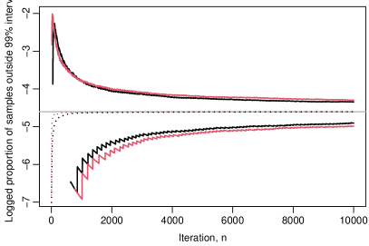
(a) Component $k=1$

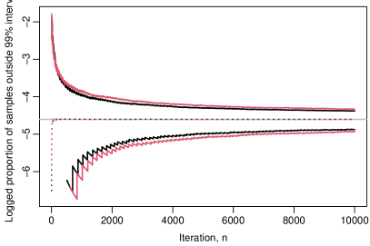
(b) Component $k=2$

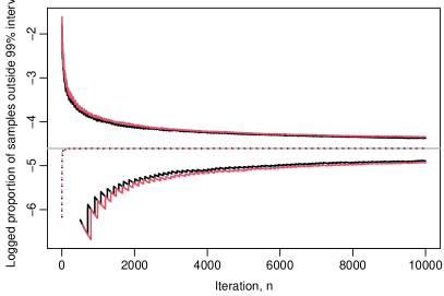
(c) Component $k=3$

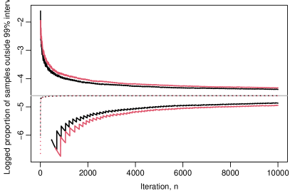
(d) Component $k=4$

(e) Component $k=5$

(f) Joint

Figure 5: Uncorrelated 5-dimensional Gaussian Target, $\varpi_{1}$: Figures (a) to (e) presents the average and 95% empirical quantiles of $\{C_{n}^{(r)}(k);r=1,\dots,R\}$ for $k=1,\dots,5$ respectively. Figure (f) present the average and 95% empirical quantiles of $\{D_{n}^{(r)};r=1,\dots,R\}$. Averages are represented by dotted lines and quantiles by solid lines. All results are presented on the log-scale. Black represents the AP method and red represents the AG2 method.

Next, we explore the performance of the adaptive MCMC algorithms for a target distribution, $\varpi_{2}$, with correlation across the components. The target distribution for this second example is taken to be a bivariate Normal distribution with mean zero and covariance matrix

$$\Sigma=\left(\begin{array}[]{cc}0.25&1.875\\ 1.875&25\end{array}\right).$$

Note that in this simulation, the component-wise MCMC proposal updates, for both the AP and AG2 method, are not aligned with the principal components of the target distribution. Therefore, this target distribution should pose a greater difficulty to sample from in comparison to the previous target, $\varpi_{1}$. The results from this simulation study are presented in Fig. 6, where we report the analogous summaries of the running empirical coverage probabilities, as for the previous example. Recall that both MCMC methods adapt independently per component. Therefore, the correlation between the components is ignored in the MCMC methods and their adaptations. Despite ignoring the correlation, both MCMC methods perform well in terms of coverage probabilities. As shown in Fig. 6, the AP method consistently outperforms the AG2 method, in terms of the width of the empirical confidence intervals.

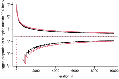
(a) Component $k=1$

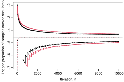
(b) Component $k=2$

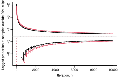
(c) Joint

Figure 6: Correlated 2-dimensional Gaussian Target, $\varpi_{2}$: Figures (a) and (b) presents the average and 95% empirical quantiles of $\{C_{n}^{(r)}(k);r=1,\dots,R\}$ for $k=1,2$ respectively. Figure (c) presents the average and 95% empirical quantiles of $\{D_{n}^{(r)};r=1,\dots,R\}$. Averages are represented by dotted lines and quantiles by solid lines. All results are presented on the log-scale. Black represents the AP method and red represents the AG2 method.

5.2 Moving to a High Density Region of Target

We now investigate the adaptive MCMC methods’ ability to move toward areas of high target density, when initially started in at a state outside that region. For this study, the target distribution is again taken as the correlated bivariate normal distribution, $\varpi_{2}$. The number of independent repetitions of the MCMC runs was again set to $R=5,000$ and the number of MCMC iterations performed each run was $N=1,000$. Each run was initialised at the location very far away from the mean, $\boldsymbol{X}_{0}=(50,50)^{T}$.

For each repetition $r$ of the MCMC method, the first time the Markov chain entered the (joint) 95% ellipse of the target is recorded as

$$J^{(r)}:=\min\left(j\in\{0,\dots,N\};(\boldsymbol{X}_{j}^{(r)})^{T}\Sigma^{-1}\boldsymbol{X}_{j}^{(r)}<z_{0}\right),$$

where $z_{0}$ is such that $P(Z_{0}>z_{0})=0.95$ and $Z_{0}\sim\chi^{2}_{2}$. The empirical distribution of the first hitting times $\{J^{(1)},\dots,J^{(R)}\}$ is summarised in the violin plots presented in Fig. 7 for AP and AG2 methods. Violin plots (Hintze and Nelson,, 1998) are boxplots with kernel density estimates attached to the sides. We use violin plots as opposed to just boxplots to give a better illustration of the shape of the distributions. In the violin plots the median is represented by a vertical line.

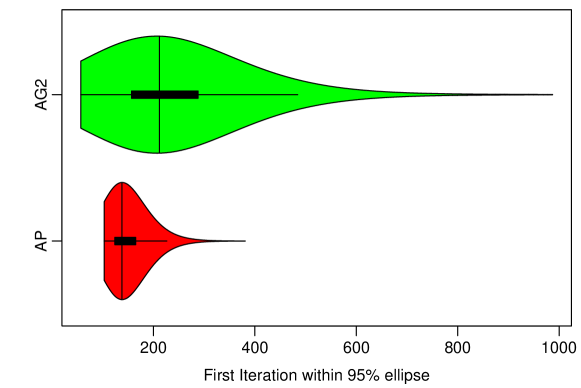
Figure 7: Correlated 2-dimensional Gaussian Target, $\varpi_{2}$: Violin plot of first hitting time of the Markov chain into 95% ellipse. AP results represented in red and AG2 results in blue.

From Fig. 7 we observe that the AP method consistently moves into the 95% ellipse earlier than the AG2 method. Although the AG2 method does enter the ellipse earlier in some iterations, the AP method always ($5,000$ out of $5,000$ iterations) entered the high-density region in less than $381$ iterations. In comparison, in $517$ out of $5,000$ iterations, the AG2 took more than $381$ iterations to enter the ellipse.

6 Results

In this section, we compare the long-term performance of the proposed adaptive component-wise, multiple-try MCMC method with other MCMC methods in simulations. The adaptive Plateau MCMC (AP) is compared a Metropolis-Hastings algorithm with Gaussian proposals (MH) and two versions of an adaptive Gaussian MCMC (AG1 and AG2)  as introduced in Yang et al., (2019). The difference between AG1 and AG2 is that AG1 uses (2) with $\alpha=2.5$ (i.e., the same weight as in AP), while AG2 uses $\alpha=2.9$ as is suggested in Yang et al., (2019). The proposal distributions in both AG1 and AG2 are adapted in the fashion outlined in Section 5.

For all simulations and methods with multiple trials we fix the number of trials $M=5$. Investigation of the methods performance for differing values of $M$ is beyond the scope of this paper, which we leave for future work. However, interesting discussions in that direction already exist, see Martino and Louzada, (2017) for example.

The proposal standard deviation in the AG1 and AG2 methods are initialised at $2^{j-2}$ for $j=1,\dots,M$. The Plateau parameters values are initialised at $\delta=\delta_{1}=1$, $\sigma=0.05$ and $\varsigma=3$ with $\eta_{1}=\eta_{2}=0.4$ for the AP method.

The proposal distributions used in the MH method depend on the particular target distribution and the choices used are summarised in Table 2 below. The various target distributions considered in the simulations are now introduced.

6.1 Target Distributions

In order to compare the aforementioned methods, we investigate their performances by applying them to sample from a variety of target distributions.

Mixture of Gaussians

Consider a mixture of two 4-dimensional Gaussians

$$\frac{1}{2}\mathrm{N}(\boldsymbol{\mu}_{1},\Sigma_{1})+\frac{1}{2}\mathrm{N}(\boldsymbol{\mu}_{2},\Sigma_{2}),$$

where

$$\boldsymbol{\mu}_{1}=(5,5,0,0)^{T},\quad\boldsymbol{\mu}_{2}=(15,15,0,0)^{T}$$

and

$$\Sigma_{1}=\text{diag}(6.25,6.25,6.25,0.01),\quad\Sigma_{2}=\text{diag}(6.25,6.25,0.25,0.01).$$

We refer to this target distribution as $\pi_{1}$.

Banana Distribution

Consider the 8-dimensional “banana-shaped” distribution (Haario et al.,, 1999), which is defined as follows. Let $f$ be the density of the $8$D normal distribution $\mathrm{N}(\boldsymbol{0},\Sigma_{3})$ with covariance given by $\Sigma_{3}=\text{diag}(100,1,\dots,1)$. The density function of the banana distribution with non-linearity parameter $b>0$ is given by $f_{b}=f\circ\phi_{b}$ where the function $\phi_{b}$ is

$$\phi_{b}(\boldsymbol{x})=(x_{1},x_{2}+bx_{1}^{2}-100b,x_{3},\dots,x_{8})\quad\text{for }\boldsymbol{x}\in\mathbb{R}^{8}.$$

The value of $b$ determines the amount of non-linearity of $\phi_{b}$. Here, we consider the target distribution $\pi_{2}=f_{0.03}$. Thus, the first 2 components of this distributions are highly correlated – see Figure 8a.

Distributions perturbed by oscillations

Another target we consider is the perturbed 2-dimensional Gaussian, whose probability density function is given by

$$\pi_{3}(\boldsymbol{x})\propto\exp\left[-\boldsymbol{x}^{T}A\boldsymbol{x}-\cos\left(\frac{x_{1}}{0.1}\right)-0.5\cos\left(\frac{x_{2}}{0.1}\right)\right]=:\widetilde{\pi}_{3}(\boldsymbol{x})\quad\text{for }\boldsymbol{x}\in\mathbb{R}^{2}$$

where

$$A=\left(\begin{array}[]{cc}1&1\\ 1&3/2\end{array}\right).$$

Figure 8c displays the un-normalised function $\widetilde{\pi}_{3}(\boldsymbol{x})$. Lastly, we also consider the following perturbed version of the 1D bi-stable distribution $x\mapsto Z^{-1}e^{-x^{2}+5x^{2}}$, whose PDF is given by

$$\pi_{4}(x)\propto\exp\left[-x^{4}+5x^{2}-\cos\left(\frac{x}{0.02}\right)\right]\quad\text{for }x\in\mathbb{R}.$$

Figure 8d displays the PDF of $\pi_{4}(x)$ where the normalising constant is approximated by numerical integration.

6.2 Run parameters

Each simulation run of the MCMC methods was independently repeated $R=200$ times and for each run a burn-in period of $50$% of the MCMC iterations was used. During the burn-in period, the AP, AG1 and AG2 were allowed to adapt their proposals. For each repetition, all methods started at the same random initial condition $\boldsymbol{x}_{0}$. The number of MCMC iterations, $N$, used for each method is presented in Table 1, which was determined by a trial run. In order to make fair comparisons, the number of MCMC iterations performed by Metropolis-Hastings algorithm is $d\times M$ times larger than the multiple-try versions. This is because multiple-try methods cycle over all $d$ components and evaluates the target for $M$ trials each iteration. This will ensure that the number of times the target distribution is evaluated by each MCMC method is exactly same and that the computational effort is approximately the same.

Target	Dimensions ($d$)	Adaptive	MH
$\pi_{1}$	4	4,000	80,000
$\pi_{2}$	8	10,000	400,000
$\pi_{3}$	2	3,000	30,000
$\pi_{4}$	1	3,000	15,000

Table 1: Number of MCMC iterations used in simulations for each target distribution.

The proposal distribution in the MH method for each target is presented in Table 2. Note that these proposals are based on the target distribution, which would be typically be unknown in practice. Consequently, the MH method can be viewed as being optimally tuned.

The particular scaling of $2.4/\sqrt{d}$ follows from Gelman et al., (1996).

Target	Proposal Distribution
$\pi_{1}$	$\displaystyle\frac{2.4}{\sqrt{4}}\left[0.5\mathrm{N}(\boldsymbol{0},\Sigma_{1})+0.5\mathrm{N}(\boldsymbol{0},\Sigma_{2})\right]$
$\pi_{2}$	$\displaystyle\frac{2.4}{\sqrt{8}}\mathrm{N}(\boldsymbol{0},\Sigma_{3})$
$\pi_{3}$	$\displaystyle\frac{2.4}{\sqrt{2}}\mathrm{N}(\boldsymbol{0},A^{-1})$
$\pi_{4}$	$\displaystyle 2.4\mathrm{N}(0,1)$

Table 2: Proposal distributions used in the Metropolis-Hastings algorithm.

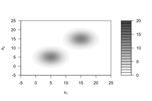
(a)

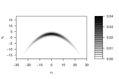
(b)

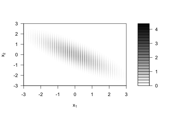
(c)

(d)

Figure 8: Selected marginal density plots of simulation target distributions

6.3 Simulation Results

For each target distribution, we compare the performance of the MCMC methods using measures which we now define. Denote the Markov chain produced by one of the MCMC methods for the $r$th independent repetition as $\boldsymbol{X}_{0}^{(r)},\dots,\boldsymbol{X}_{N}^{(r)}$ where $\boldsymbol{X}_{i}^{(r)}=(X_{i,1}^{(r)},\dots,X_{i,d}^{(r)})^{T}$ for $r=1,\dots,R$. Denote the component-wise variances of the target $\pi$ as $\sigma_{1}^{2},\dots,\sigma_{d}^{2}$.

We will use the integrated autocorrelation time (ACT) of the MCMC methods as a measure of performance. The ACT for the chain’s $k$th component is given by

$$\mathrm{ACT}_{k}=1+\frac{2}{\sigma^{2}_{k}}\sum_{i=1}^{N}\text{cov}(X_{0,k},X_{i,k})\;,$$

provided that the chain is stationary so that $\boldsymbol{X}_{0}\sim\pi$. For every repetition $r=1,\dots,R$ of the MCMC method, the integrated autocorrelation times are estimated based on the observed Markov chain $\boldsymbol{X}_{0}^{(r)},\dots,\boldsymbol{X}_{N}^{(r)}$ component-wise using the initial sequence estimator introduced in Geyer, (1992). With slight abuse of notation, we will denote the resulting chain-based autocorrelation times by $\mathrm{ACT}_{k}^{(r)}$. Smaller autocorrelation times indicate that consecutive samples have lower correlation. Autocorrelation times are inversely proportional to the effective sample size Kong, (1992); Kong et al., (1994), which is commonly used as a measure of performance. In fact, the effective sample size is often interpreted as the number of samples that would need to be (directly) drawn from the target in order to achieve the same variance as that from an estimator of interest using independent samples. Higher effective sample sizes and therefore lower autocorrelation times are desirable. Another way of interpreting the ACTs is through the accuracy of a chain-based Monte Carlo integration. As a matter of fact, the mean squared error of a Monte Carlo estimator can be expressed as a sum of the component-wise ACTs weighted by the component-wise variance. Consequently, a method with lower ACTs will offer more accurate Monte Carlo integration for the same chain length. It is moreover noteworthy that an MCMC method’s ACTs also characterise the asymptotic variance (so-called time-averaged variance constant in this context) of an Monte Carlo estimator in the central limit theorem for Markov chains (see e.g. Asmussen and Glynn,, 2007). In fact, lower ACTs will lead to smaller time-averaged variance constants. Finally, we mention that in practice, the target distribution is intractable and therefore the variances of the components are unknown. However, these variances can be estimated by the initial sequence estimator method.

Another measure of performance is the chain’s average squared jump distance (ASJD), which, for the $k$th component and repetition $r$, we define as

$$\mathrm{ASJD}_{k}^{(r)}=\frac{1}{N}\sum_{i=1}^{N}|X_{i,k}^{(r)}-X_{i-1,k}^{(r)}|^{2}.$$

The average squared jump distance measures the movement of the chain and also is linked with the acceptance rate of the MCMC method. Higher values of average squared jump distances are desired as it indicates larger moves and therefore more exploration of the space. We shall consider the ASJD as a measure of a MCMC method to move around the state-space.

In summary, in the following results we are interested in the ACTs and the ASJD per component. The distribution of the ACTs and ASJDs over the repetitions, i.e. $\{\mathrm{ACT}_{k}^{(r)}:r=1,\dots,R\}$ and $\{\mathrm{ASJD}_{k}^{(r)}:r=1,\dots,R\}$, will be presented using violin plots.

6.3.1 Mixture of Gaussians

The results for the 4-dimensional mixture of two Gaussians target, $\pi_{1}$, are presented in Fig. 9. Fig. 9a indicates that the AP method achieves lower ACTs than the other methods for all components (including the MH method which is not included in this figure due to very high ACTs). Further, the range of ACT values suggest that the AP method consistently produces MCMC chains with lower ACTs.

In terms of the movement of the MCMC chains, the AP method outperforms the other methods for this target distribution. In fact, the ASJDs presented in Fig. 9b show that the AP method moving around the state-space in larger jumps than the other methods. Since the AP and AG1 methods use the same weight function as discussed in Section 2.1 this advantage is due to using the Plateau proposals in contrast to Gaussian proposals. These results suggest that the AP method is able to move between the two Gaussians in the target density efficiently.

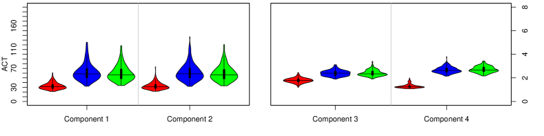
(a) Autocorrelation times

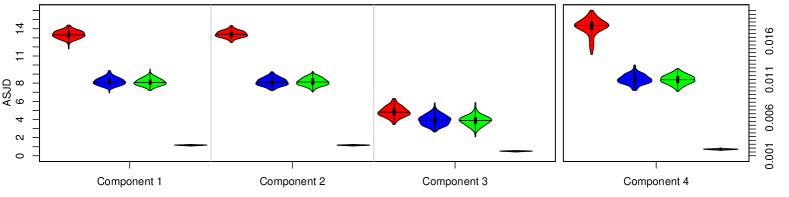
(b) Average square jump distance

Figure 9: Mixture of Gaussians, $\pi_{1}$: Distribution of the ACTs and ASJDs of MCMC methods for target $\pi_{1}$. Red is AP, blue is AG1, green is AG2 and pink is MH.

6.3.2 Banana Distribution

The target, $\pi_{2}$, is a difficult distribution to sample from due to the wide ranging variances in each component and the unusual banana-shape of the first two components. The ACTs for the methods, presented in Fig. 10a, show similar results across the AP, AG1 and AG2 for the first two components. However, the remaining components the AP is achieving notably smaller ACTs. The ACT results for the MH are substantially larger for all components and thus are not included in this figure. As an indication, the median ACTs for components 1 to 8 respectively are: 1131.74, 2066.35, 54.24, 54.37, 54.34, 54.03, 54.74, 54.47 for the MH method to 2 decimal places.

The ASJDs for the methods presented in Fig. 10b. The AP method again outperforms the other methods by achieving higher ASJDs for all components. Note that for the first component the wide range of jumping distance produced when using the Plateau proposals. This suggests that the AP method is able to navigate the banana-shape in the first component easily.

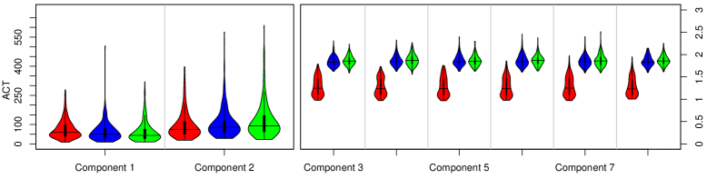
(a) Autocorrelation times

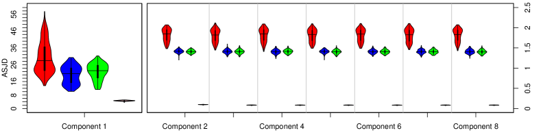
(b) Average square jump distance

Figure 10: Banana Distribution, $\pi_{2}$: Distribution of the ACTs and ASJDs of MCMC methods for target $\pi_{2}$. Red is AP, blue is AG1, green is AG2 and pink is MH.

6.3.3 2D Perturbed Distribution

For the perturbed 2-dimensional distribution, $\pi_{3}$, the perturbations represent local modes where MCMC methods may potentially get stuck. Again, the AP method’s ability to move slightly larger distances, as shown in Fig. 11b, gives it a slight advantage over the other methods. This ability to jump further may explain the lower ACTs for the AP method as depicted in Fig. 11a.

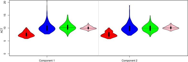
(a) Distribution of log autocorrelation times

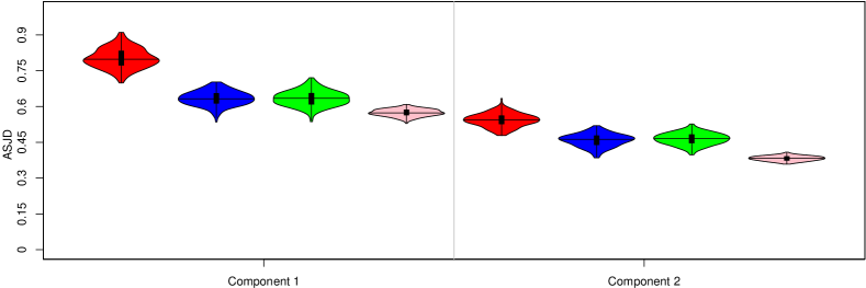
(b) Distance of average square jump distance

Figure 11: 2D Perturbed Distribution, $\pi_{3}$: Distribution of the ACTs and ASJDs of MCMC methods for target $\pi_{3}$. Red is AP, blue is AG1, green is AG2 and pink is MH.

6.3.4 1D Perturbed Distribution

Similar to $\pi_{3}$, the oscillations in $\pi_{4}$ are potential areas where an MCMC may get stuck. The ACTs for the AP, AG1 and AG2 method are presented in Fig. 12a. The AP achieves the lowest ACTs, however there are a few outliers which may indicate a few runs where the sampler got stuck in the local modes. This may also be the case for the AG1 method. For the MH method, the ACTs (not presented in the figure) are extremely large in comparison to the the other methods – with a median of 178.54 and a range of $(111.62,457.56)$ to 2 decimal places.

The ASJDs for the AP method, on average is jumping also twice the distance of the AG1 and AG2 methods – see Fig. 12b. Again there are some outlying ASJDs for the AP method which may indicate some repetitions where the MCMC got stuck in local modes.

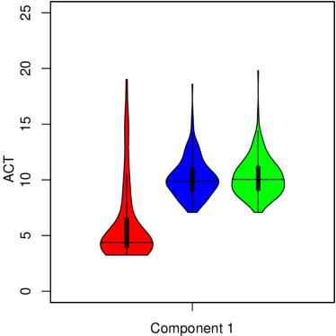
(a) Distribution of autocorrelation times

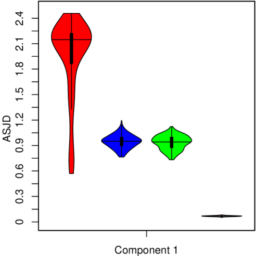
(b) Distribution of average square jump distance

Figure 12: 1D Perturbed Distribution, $\pi_{4}$: Distribution of the ACTs and ASJDs of MCMC methods for target $\pi_{4}$. Red is AP, blue is AG1, green is AG2 and pink is MH.

7 Conclusion

In this paper we have introduced Plateau distributions as a novel-class of proposal distributions for the use with component-wise, multiple-try Metropolis MCMC. These proposal distributions are a combination of uniform distributions, leading to a family of distributions with non-overlapping supports. The notion of using non-overlapping proposals in multiple-try MCMC methods is intuitive and, in fact, motivated as means to counter the disadvantages (e.g. inefficient proposing of trials) of greatly overlapping proposal distributions such as Gaussians. Moreover, the class of Plateau distributions are simple to implement for use as proposals in MCMC methods and are straightforwardly combined with the simple, yet highly effective, adaptation procedure presented in Section 4. As mentioned in the introduction, the novelty of this work lies in both the Plateau proposals and the bespoke adaptation method. The designed adaptation method takes advantage of the non-overlapping proposals to better explore the space and “scale” the proposals to the target distribution. The advantages of our proposed algorithm over Gaussian proposals with a similar adaptation method was presented in simulations in Section 5.

We have demonstrated that using the Plateau proposal distributions with the suggested adaptation leads to MCMC methods that perform well for a variety of target distributions. In fact, the results indicate that using our method produces MCMC chains that explore the state-space better with lower autocorrelation times, when compared to other adaptive multiple-try methods with greatly overlapping Gaussian proposals. Furthermore, the simulation results suggest that the Plateau proposals are able to efficiently sample from target distributions with distance modes, complex shapes, and many nearby modes.

The results and the simplicity of their design makes the Plateau proposals appealing for general use in component-wise, multiple-try MCMC algorithms. As a matter of fact, the introduced class of Plateau distributions is one type of non-overlapping proposals. Further research may investigate other types of non-overlapping proposals which may have multiple interacting trials (e.g. see Casarin et al., (2013)) and may be asymmetric. Further theoretical research is required to determine the mixing properties of the MCMC chain produced by these Plateau proposals and adaptation procedure.

Appendix A A note of convergence of adaptive component-wise multiple-try algorithms

The convergence (in total variation distance) of algorithms of the form of Algorithm 1 described in Section 4 has been proven in Yang et al., (2019).

The proof of convergence is ensured by the algorithm, both the MCMC algorithm and the adaptation procedure, satisfying two conditions: diminishing adaptation and containment. As mentioned earlier, diminishing adaptation is satisfied by adapting with probability $P_{n}=\max\left\{0.99^{n-1},1/\sqrt{n}\right\}$. For containment to hold two technical, but not practical, modifications are required – these follow directly from Yang et al., (2019) and are presented as quotations below with altered notation. The first modification is to

“ … choose a very large nonempty compact set $K\subset\mathcal{X}$ and force $\boldsymbol{X}_{n}\in K$ for all $n$. Specifically, we reject all proposals $\boldsymbol{Y}\notin K$ (but if $\boldsymbol{Y}\in K$, then we still accept/reject $\boldsymbol{Y}$ by the usual rule)… ”

The second modification which is altered for our proposed Plateau distributions is

“ … choose a very large constant $\Delta$ and a very small constant $\epsilon>0$ and force the proposal width $\delta$ to always be in $[\epsilon,\Delta]$… ”

The proof then follows Section 3.5 in Yang et al., (2019).

References

- Asmussen and Glynn, (2007) Asmussen, S. and Glynn, P. W. (2007). Stochastic Simulation: Algorithms and Analysis. Springer.
- Brooks et al., (2011) Brooks, S., Gelman, A., Jones, G. L., and Meng, X.-L., editors (2011). Handbook of Markov chain Monte Carlo. CRC Press.
- Casarin et al., (2013) Casarin, R., Craiu, R., and Leisen, F. (2013). Interacting multiple try algorithms with different proposal distributions. Statistics and Computing, 23(2):185–200.
- Casella and George, (1992) Casella, G. and George, E. I. (1992). Explaining the gibbs sampler. The American Statistician, 46(3):167–174.
- Craiu and Lemieux, (2007) Craiu, R. V. and Lemieux, C. (2007). Acceleration of the Multiple-Try Metropolis algorithm using antithetic and stratified sampling. Statistics and Computing, 17(2):109–120.
- Gelman et al., (1996) Gelman, A., Roberts, G., and Gilks, W. (1996). Efficient Metropolis jumping rules. Bayesian statistics, 5(599-608):42.
- Geyer, (1992) Geyer, C. J. (1992). Practical Markov chain Monte Carlo. Statistical Science, 7(4):473–483.
- Gilks et al., (1995) Gilks, W. R., Richardson, S., and Spiegelhalter, D. (1995). Markov chain Monte Carlo in practice. Chapman and Hall/CRC.
- Giordani and Kohn, (2010) Giordani, P. and Kohn, R. (2010). Adaptive independent Metropolis-Hastings by fast estimation of mixtures of normals. Journal of Computational and Graphical Statistics, 19(2):243–259.
- Haario et al., (1999) Haario, H., Saksman, E., and Tamminen, J. (1999). Adaptive proposal distribution for random walk Metropolis algorithm. Computational Statistics, 14(3):375–395.
- Haario et al., (2001) Haario, H., Saksman, E., and Tamminen, J. (2001). An adaptive Metropolis algorithm. Bernoulli, 7(2):223–242.
- Hastings, (1970) Hastings, W. K. (1970). Monte Carlo sampling methods using Markov chains and their applications. Biometrika, 57(1):97–109.
- Hintze and Nelson, (1998) Hintze, J. L. and Nelson, R. D. (1998). Violin plots: A box plot-density trace synergism. The American Statistician, 52(2):181–184.
- Jun S. Liu, (2000) Jun S. Liu, Faming Liang, W. H. W. (2000). The multiple-try method and local optimization in Metropolis sampling. Journal of the American Statistical Association, 95(449):121–134.
- Kong, (1992) Kong, A. (1992). A note on importance sampling using standardized weights. University of Chicago, Dept. of Statistics, Technical Report, 348.
- Kong et al., (1994) Kong, A., Liu, J. S., and Wong, W. H. (1994). Sequential imputations and Bayesian missing data problems. Journal of the American Statistical Association, 89(425):278–288.
- Martino and Louzada, (2017) Martino, L. and Louzada, F. (2017). Issues in the multiple try metropolis mixing. Computational Statistics, 32(1):239–252.
- Martino and Read, (2013) Martino, L. and Read, J. (2013). On the flexibility of the design of multiple try Metropolis schemes. Computational Statistics, 28(6):2797–2823.
- Metropolis et al., (1953) Metropolis, N., Rosenbluth, A. W., Rosenbluth, M. N., Teller, A. H., and Teller, E. (1953). Equation of state calculations by fast computing machines. The Journal of Chemical Physics, 21(6):1087–1092.
- Neal et al., (2011) Neal, R. M. et al. (2011). Mcmc using hamiltonian dynamics. In Brooks, S., Gelman, A., Jones, G., and Meng, X.-L., editors, Handbook of Markov chain Monte Carlo. CRC press.
- Roberts and Rosenthal, (2001) Roberts, G. O. and Rosenthal, J. S. (2001). Optimal scaling for various Metropolis-Hastings algorithms. Statistical Science, 16(4):351–367.
- Roberts and Rosenthal, (2007) Roberts, G. O. and Rosenthal, J. S. (2007). Coupling and ergodicity of adaptive Markov chain Monte carlo algorithms. Journal of Applied Probability, 44(2):458–475.
- Roberts and Tweedie, (1996) Roberts, G. O. and Tweedie, R. L. (1996). Exponential convergence of Langevin distributions and their discrete approximations. Bernoulli, 2(4):341–363.
- Rosenthal, (2011) Rosenthal, J. S. (2011). Optimal proposal distributions and adaptive MCMC. In Brooks, S., Gelman, A., Jones, G., and Meng, X.-L., editors, Handbook of Markov chain Monte Carlo. CRC press.
- Yang et al., (2019) Yang, J., Levi, E., Craiu, R. V., and Rosenthal, J. S. (2019). Adaptive component-wise multiple-try Metropolis sampling. Journal of Computational and Graphical Statistics, 28(2):276–289.