Dependency-Aware Named Entity Recognition with
Relative and Global Attentions

Abstract

Named entity recognition is one of the core tasks in NLP. Although many improvements have been made on this task during the last years, the state-of-the-art systems do not explicitly take into account the recursive nature of language. Instead of only treating the text as a plain sequence of words, we incorporate a linguistically-inspired way to recognize entities based on syntax and tree structures. Our model exploits syntactic relationships among words using a Tree-LSTM guided by dependency trees. Then, we enhance these features by applying relative and global attention mechanisms. On the one hand, the relative attention detects the most informative words in the sentence with respect to the word being evaluated. On the other hand, the global attention spots the most relevant words in the sequence. Lastly, we linearly project the weighted vectors into the tagging space so that a conditional random field classifier predicts the entity labels. Our findings show that the model detects words that disclose the entity types based on their syntactic roles in a sentence (e.g., verbs such as speak and write are attended when the entity type is PERSON, whereas meet and travel strongly relate to LOCATION). We confirm our findings and establish a new state of the art on two datasets.

1 Introduction

In the study of the named entity recognition (NER) task, neural sequence labeling models have been vastly explored by the NLP community. Small variations aside, the majority of these models use a combination of a bidirectional LSTM and conditional random fields (CRF) to reach state of the art performance (Lample et al., 2016; Ma and Hovy, 2016; Peng and Dredze, 2016b; Jie Yang and Zhang, 2018; Aguilar et al., 2018). Recently, transfer learning from pre-trained language models has played an important role on improving the performance even further (Liu et al., 2017; Peters et al., 2018; Akbik et al., 2018; Devlin et al., 2018; Howard and Ruder, 2018). However, these NER models mainly consider the text as a plain sequence of words without explicitly taking into account the recursive nature of language. Consider the phrase in Figure 1, “Your friend Jason, who has been helping us, called you using his new Samsung.” The main sentence is composed of a verb phrase whose head is called, which in turn includes another verb phrase headed by the word using. In addition to this, such recursive properties can produce more involved and longer sentences. This behavior can potentially obscure relationships among words when the text is treated as a linear chain of tokens. For instance, in the same example, the words Jason, called, using, and Samsung easily describe the way in which the entities Jason and Samsung interact. Nevertheless, existing models struggle identifying such relationships in long sentences, resulting in a drop in performance.

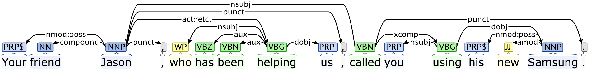
Figure 1: A dependency tree that shows how words relate among each other. It is worth noting that the connections called $\rightarrow$ Jason and called $\rightarrow$ using $\rightarrow$ Samsung capture how the entities Jason and Samsung interact. While the verb called provides clues to the fact that Jason is a person, the verb using and the adjective new suggest that Samsung is a product and not a company.

We propose a new approach for NER where the goal is to enhance the syntactic relationships among words and combine such aspects with semantic representations commonly used in this task. Our model extracts features from text using a Tree-LSTM Tai et al. (2015) guided by dependency tree structures. As shown in Figure 1, the dependency trees connect the words based on the role they play in the sentence and the way they interact with each other. The output features are weighted with relative and global attention mechanisms. While the relative attention focuses on the most relevant words with respect to the word being evaluated, the global attention spots the most important words over the sentence as a whole. After weighting the hidden vectors, we linearly project them into the tagging space. We predict the entity labels using a conditional random field classifier. Our findings show that the model detects words that disclose the entity types based on their syntactic roles in a sentence (e.g., verbs such as speak and write are attended when the entity type is PERSON, whereas meet and travel strongly relate to LOCATION).

The contribution of this work can be summarized as follows: we (a) apply global and relative attentions to detect informative word relationships, (b) provide an end-to-end architecture that involves language model, Tree-LSTM, attention mechanisms, and CRF, (c) derive insights from entity and word correlations learned by the model, (d) release the entire project that allows replicability of all the described experiments and analysis, and (e) establish a new state of the art on the OntoNotes 5.0 Broadcast News section, and SemEval 2010 Task 1 datasets.

2 Related Work

Recursive neural networks started to be considered in computer vision to target the compositionality problem. Socher et al. (2011) combined fragments of images associated to constituencies in binary parsing trees to extract composed features using recursive neural networks. However, the main problem was that their model did not retain the information along the tree but it only captured the immediate comparison between adjacent nodes. Matrix-vector models aimed at keeping long term information with a reasonable performance Socher et al. (2012), but Tai et al. (2015) proposed a more feasible way to overcome the compositionality problem. They introduced the multi-purpose Tree-LSTM architecture that generalizes the standard LSTM Hochreiter and Schmidhuber (1997). The Tree-LSTM model is capable to handle N-ary trees using dynamic batching. They also improved the state of the art in sentiment analysis at that point in time, which shows the potential of modeling linguistic problems recursively. We follow the implementation of Child-Sum Tree-LSTM to extract syntactic features guided by dependency trees.

Dependency parses have been hardly employed on NER. Recently, Jie et al. (2017) explored this line of research with slightly different focus. They concentrate on efficient models that show less running time by using a semi-Markov CRF to exploits dependency features. We compare our model with their work since their approach also extracts features using Tree-LSTM on dependency trees. Additionally, Feng et al. (2017) proposed a deep reinforcement learning framework where the goal is recognize entities and extract their relations simultaneously. They identify a candidate pair of entities using LSTM and an attention mechanism, then they employ a Tree-LSTM to extract the entity relation using the path between the pairs in a dependency tree. They use this information in a Q-learning algorithm to optimize the policy of their system. Unlike them, we use the dependency trees to extract syntactic features that describe the interaction between entities and the rest of the words, regardless if they are other entities. This allows us to find words that disclose entity type information according to the sentence syntactic structure (e.g., verbs that only PERSON entities perform).

We enhance our syntactic features using two different attention mechanisms. Attention was introduced by Bahdanau et al. (2014) in the task of machine translation. Since then, it has been broadly used in many other applications such as semantic slot filling (Zhang et al., 2017) and sentiment analysis. We employ a similar attention component, which we call global attention (see Section 3.2.3). More recently, Vaswani et al. (2017) proposed the transformer architecture, which contains a multi-head self-attention module. Our relative attention mechanism is very similar to this module, but the main difference is that, for a word $w_{i}$ in a sentence, we draw the probability distribution over the words $w_{j}$ where $i\neq j$ (see Section 3.2.2). Additionally, the transformer architecture has been used in the language model BERT Devlin et al. (2018), which is benchmarked on NER.

NER has evolved rapidly in the last years. While the standard architectures involve a combination of BLSTMs with a CRF classifier Lample et al. (2016); Limsopatham and Collier (2016); Chieu and Ng (2003); Peng and Dredze (2016a); Chiu and Nichols (2016); Aguilar et al. (2018), recent advances have improved those approaches with transfer learning from pretrained language models such as ELMo Peters et al. (2018) and BERT Devlin et al. (2018). These language models show a similar performance on the CoNLL 2003 benchmark, but the current state of the art on this dataset is the contextual string embeddings from language models proposed by Akbik et al. (2018). We take advantage of such improvements by using ELMo to generate our contextualized word representations.

3 Methodology

This section describes the feature representation, the model architecture, and the training details.

3.1 Feature representation

We represent the input data using words, part-of-speech tags, and dependency parses. For words, we employ deep contextualized representations using the language model ELMo (Peters et al., 2018). ELMo provides vector representations that are entirely built out of characters. This allows us to overcome the problem of out-of-vocabulary words by always having a vector based on morphological clues for any given token. For POS tags and dependency relations, we use trainable embedding matrices that are optimized from scratch. POS tags have proven useful in previous research Chiu and Nichols (2016); Aguilar et al. (2018), and dependency relations help the model to infer the interaction between nodes in the trees. Once we have a vector representation for every input feature, we concatenate them to form a single vector for every token in the sentence.

3.2 Model architecture

We describe the components of our model individually, and then we discuss the overall architecture.

3.2.1 Tree-LSTM

The Tree-LSTM component, introduced as Child-Sum Tree-LSTM by Tai et al. (2015), is a generalization of the standard LSTM cell Hochreiter and Schmidhuber (1997) that can handle multiple inputs at every time step. In fact, both cells are equivalent when the input tree is comprised of a single child at every level. The equations are as follows:

$$\begin{split}\tilde{h}_{j}=&~{}\sum_{k\in C(j)}h_{k}\\ i_{j}=&~{}\sigma(\mathrm{W}^{(i)}x_{j}+\mathrm{U}^{(i)}\tilde{h}_{j}+b^{(i)})\\ f_{jk}=&~{}\sigma(\mathrm{W}^{(f)}x_{j}+\mathrm{U}^{(f)}h_{k}+b^{(f)})\\ o_{j}=&~{}\sigma(\mathrm{W}^{(o)}x_{j}+\mathrm{U}^{(o)}\tilde{h}_{j}+b^{(o)})\\ u_{j}=&~{}\mathrm{tanh}(\mathrm{W}^{(u)}x_{j}+\mathrm{U}^{(u)}\tilde{h}_{j}+b^{(u)})\\ c_{j}=&~{}i_{j}\odot u_{j}+\sum_{k\in C(j)}f_{jk}\odot c_{k}\\ h_{j}=&~{}o_{j}\odot\mathrm{tanh}(c_{j})\\ \end{split}$$

where $k\in C(j)$, and $C(j)$ determines the children of the node $j$. The differences are that, in a given time step (i.e., node), the forget cell $f_{jk}$ is calculated for every hidden input state $h_{k}$, and the cell state $c_{j}$ is the sum of the products between $f_{jk}$ and $c_{k}$ for every child $k$ of node $j$. In our case, the dependency trees consist of words at every node. That is, the input $x_{j}$ is an embedding vector representing a word $w_{j}$. Its children are the words $w_{k}$ which produce the $h_{k}$ hidden states. Since children are used as input to the next node, the Tree-LSTM model runs in a bottom-up fashion. In the case of multi-rooted phrases, we simply average the root vectors to come up with a single last hidden state $h_{root}$.

3.2.2 Relative attention

The goal of the relative attention is to produce a Cartesian product of probabilities based on the words in the sentence, where the main diagonal is not taken into account to draw the probability distribution. This is slightly different from the self-attention mechanism proposed by Vaswani et al. (2017) in that we draw the probability distribution over the words $w_{j}$ of the sentence for every word $w_{i}$, where $i\neq j$, as opposed to distributing the probabilities over all the words regardless. We use the scaled-dot product function to produce the attention matrix. That is, we scale the weights by the inverse square root of their embedding dimension, mask out the main diagonal of such scores, and normalize the result using a softmax function:

$$A=~{}\mathrm{softmax}(d^{-0.5}_{a}QK^{T})$$ (1)

where $A\in\mathbb{R}^{N\times N}$ is a squared matrix that contains the attention weights for $N$ words in a sentence, $i$ and $j$ denote the row and column indexes, such that $\sum_{i}^{N}\sum_{j\neq i}^{N}A_{ij}=N$. $Q$ and $K$ are linear transformations of the input using the query and key matrices $\mathrm{W}_{Q}\in\mathbb{R}^{d_{a}\times d_{a}}$ and $\mathrm{W}_{K}\in\mathbb{R}^{d_{a}\times d_{a}}$ where $d_{a}$ is the dimension of the input and output matrices. The weighted values are calculated as follows:

$$M=~{}AV+V$$ (2)

Similar to $Q$ and $K$, $V$ is a linear projection of the input using the value matrix $\mathrm{W}_{V}\in\mathbb{R}^{d_{a}\times d_{a}}$. Note that the matrix multiplication between $A$ and $V$ discards the words $w_{ii}$ because $A$ contains zeros in its main diagonal. Hence, we include this information by adding the matrix $V$ to such product.

3.2.3 Global attention

In the case of the global attention, we use a fairly standard mechanism introduced by Bahdanau et al. (2014). The idea is to concentrate mass probability over the words that capture the most relevant information along the sentence. Our attention mechanism uses the following equations:

$$\begin{split}u_{i}=&~{}v^{\intercal}~{}\mathrm{tanh}(\mathrm{W}_{h}h_{i}+b_{h}+\mathrm{W}_{q}q+b_{q})\\ a_{i}=&~{}\frac{\mathrm{exp}(u_{i})}{\sum^{N}_{j=1}\mathrm{exp}(u_{j})},~{}~{}~{}\text{s.t.}~{}\sum_{i=1}^{N}a_{i}=1\\ z_{i}=&~{}a_{i}h_{i}\end{split}$$ (3)

where $\mathrm{W}_{h}\in\mathbb{R}^{d_{a}\times d_{h}}$, $\mathrm{W}_{q}\in\mathbb{R}^{d_{a}\times d_{q}}$, $b_{h}\in\mathbb{R}^{d_{a}}$, and $b_{q}\in\mathbb{R}^{d_{a}}$ are learnable parameters of the model. $\mathrm{W}_{h}$ and $\mathrm{W}_{q}$ are used to linearly project the hidden word vectors $h_{i}$ and the query vector $q$ into the attention space. The vector $v\in\mathbb{R}^{d_{a}}$ is the attention vector to be learned. $d_{h}$, $d_{q}$, and $d_{a}$ are the dimensions of the hidden word vectors, the query vector, and attention layer, respectively. Note that the query vector $q$ is a context vector that summarizes the entire sentence. In the case of using a Tree-LSTM, $q$ is the root hidden vector $h_{root}$, whereas in a LSTM $q$ is simply the last hidden state $h_{n}$. Finally, we multiply the scalars $a_{i}$ and their corresponding hidden vectors $h_{i}$ to obtain our weighted sequence $z$.

3.2.4 Residual connections

We incorporate residual connections He et al. (2015) at every component of our module, followed by layer normalization as in Ba et al. (2016). The output of a given $\mathrm{Sublayer}$ is described as follows:

$$z=\mathrm{LayerNorm}(x+\mathrm{Sublayer}(x))$$ (4)

where $\mathrm{LayerNorm}$ is an affine function that contains trainable parameters. Additionally, $\mathrm{Sublayer}$ can be any component of our model, such as a Tree-LSTM, relative attention, or global attention. We keep the same dimensions for inputs and outputs to simplify adding the vectors of any given module. This module only normalizes the output tensor in the last dimension.

3.2.5 Conditional random field

We use a conditional random field (CRF) classifier at the top of our model to perform the sequential inference. The CRF takes vectors in the tagging space as input and produces the best sequence of labels using the Viterbi algorithm. CRF is well-known and widely used for sequence labeling because it learns the rules of transitioning from one label to another based on the feature vectors of the sequence as a whole instead of individually.

Consider the observation sequence of vectors $\mathbf{x}=[x_{1},\dots,x_{n}]$ and its corresponding target labels $\mathbf{y}=[y_{1},\dots,y_{n}]$. CRF computes the conditional probability of the target sequence $\mathbf{y}$ given the inputs $\mathbf{x}$ by globally normalizing the target score:

$$\begin{split}p_{\theta}(\mathbf{y}|\mathbf{x})=&~{}\frac{1}{\mathbf{Z}_{\theta}(\mathbf{x})}\prod_{t=1}^{N}\psi(y_{t-1},y_{t},\mathbf{x};\theta)\end{split}$$ (5)

where $\mathbf{Z}_{\theta}(\mathbf{x})$ is a normalization term that adds up the products of $\psi(\cdot)$ for all the possible $\mathbf{y}$ sequences. $\psi(\cdot)$ is the potential parametric function that sums the transition and emission features. We use the logistic expression of Equation 5 during training to optimize our model (see Section 3.3).

3.2.6 Overall architecture

In this section we describe the overall architecture of our model using the previous components. As shown in Figure 2, we first embed the input sentence into a vector space using the token embedder module. This module is in charge of concatenating the word, POS tag, and dependency relationship vectors into a single representation for every token (see Section 3.1). We feed the embedded output into the semantic (on the left) and syntactic (on the right) feature extractors, which are a stacked layers of bidirectional LSTMs and Tree-LSTMs, respectively. Then, we concatenate the outputs of these components and feed them into the relative and global attention modules. The weighted vectors generated by the attention mechanisms are linearly projected into the tagging space and fed into a conditional random field classifier. The arrows that skip layers denote the residual connections.

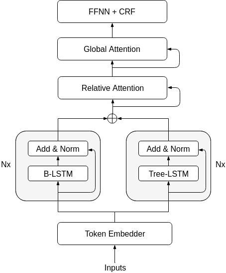
Figure 2: The overall model architecture.

3.3 Training

We optimize our model by minimizing the negative log-likelihood loss produced by the forward algorithm in the CRF module. In addition to this loss, we include an $\ell_{2}$ regularization term that targets the parameters of the semantic and syntactic feature extractors and the attention mechanisms. The idea is to reduce over-fitting when the model selects the features from the syntactic and semantic blocks, and to force the attention mechanisms to avoid bias towards specific aspects of the sentences. Given the target sequence $\mathbf{y}$ and the predicted labels $\mathbf{\hat{y}}$, we define the objective function of our model as follows:

$$\mathcal{L}= ~{}-\frac{1}{N}\sum_{i}^{N}y_{i}log(\hat{y}_{i})+\lambda\sum_{k}{w_{k}^{2}}$$ (6)

where $N$ is the length of the sentence and $w_{k}$ denotes the parameters of the feature extractors and the attention mechanisms. $\lambda$ is the penalty that indicates how much of this regularization term will be added to the overall loss, and $log(\hat{y_{i}})$ is determined by the logistic expression from Equation 5.

We reduce the loss of our model using Stochastic Gradient Descent (SGD) with momentum Sutskever et al. (2013). We train our models for 150 epochs and change the learning rate every epoch using cosine annealing and warm restarts Loshchilov and Hutter (2016). Besides adding $\ell_{2}$ regularization, we also prevent over-fitting by applying input variational dropout Gal and Ghahramani (2015) to every component in our model. Appendix A includes all the details regarding hyperparameter tuning.

Corpus	Train	Dev	Test	NEs
CoNLL 2003	14,041	3,250	3,453	4
SemEval 2010	3,648	741	1,141	22
CoNLL 2012	115,310	15,680	12,217	18
OntoNotes 5.0	9,723	1,172	1,252	18

Table 1: The data splits on each corpus along with the number of named entities.

4 Experimental results

Model Approach	CoNLL	SemEval	ON 5.0
	2003	2010	(BN)
Baselines
TlstmWord	86.72	79.53	82.20
TlstmWord+POS	88.91	84.07	88.41
TlstmWord+POS+Dep	89.20	84.89	88.67
BlstmWord	89.06	80.81	83.30
BlstmWord+POS	91.22	80.31	84.58
BlstmWord+POS+Dep	90.98	81.23	83.24
Stacked Layers
Tlstm	91.22	85.01	88.08
Tlstm${\dagger}$	91.24	85.75	88.71
Blstm	91.68	84.32	88.48
Blstm${\dagger}$	91.71	85.21	88.77
Attention
Tlstm + RA${\dagger}$	91.13	84.94	88.11
Tlstm + GA${\dagger}$	90.62	85.09	89.02
Tlstm + RA + GA${\dagger}$	90.60	86.24	88.79
Blstm + RA${\dagger}$	91.65	84.19	88.51
Blstm + GA${\dagger}$	91.39	84.87	88.39
Blstm + RA + GA${\dagger}$	91.63	85.12	88.66
Tlstm + Blstm	91.17	86.49	89.22
+ RA + GA${\dagger}$

Table 2: The averaged F1 scores of two runs on the validation sets. Blstm and Tlstm are bidirectional and tree LSTMs. The baselines specify the input features; the rest of the experiments use all the features. ${\dagger}$ denotes residual connections on every component. RA and GA refer to relative and global attentions. All the experiments use ELMo embeddings and CRF.

Dataset	Last F1 SOTA	Our F1
CoNLL-03	93.18 Akbik et al. (2018)	91.90$\pm$0.08
	92.8 Devlin et al. (2018)
	92.22 Peters et al. (2018)
SemEval-10	75.50 Jie et al. (2017)	86.72$\pm$0.11
CoNLL-12	89.30 Akbik et al. (2018)	89.07$\pm$0.15
	86.28 Chiu and Nichols (2016)
ON 5.0 (BN)	80.50 Jie et al. (2017)	89.22$\pm$0.28

Table 3: Comparison of our best F1 results and the state of the art reported on the test set of each corpus. Our model exceeds previous scores on SemEval 2010 and the OntoNotes 5.0 (BN), and it is competitive with the scores on CoNLL 2012.

We run experiments on CoNLL 2003 Tjong Kim Sang and De Meulder (2003), SemEval 2010 Task 1 Recasens et al. (2010), CoNLL 2012 Pradhan et al. (2013), and the Broadcast News section of OntoNotes 5.0 Weischedel et al. (2013). Table 1 shows a summary of the data splits for each corpus along with the number of entities (more details in Appendix B). The scores on the test set for each dataset are reported in Table 3.

4.1 Ablation analysis

Table 2 shows a systematic way to incorporate the components of our model. Based on those results, we can infer the impact of adding a component to the final architecture. For the input features, we observe that adding POS tags improves significantly the performance compared to only using the words in either Blstm or Tlstm. This is consistent with previous research (see Section 3.1). An additional small improvement can be achieved by incorporating the dependency relation labels. It is worth noting that, while the Blstm_Word or Tlstm_Word are similar in performance, the latter significantly overpasses the former when POS tags are added. Intuitively, the POS tags refine the syntactic patterns extracted from the tree structures and clarify the roles that the words play in the sentence.

For the model components, we experiment with stacked layers on the Blstm and Tlstm models (see Table 2). While there is no significant improvement over the single-layer models, we see gains when we add residual connections between each layer. The residual connections allow the model to decide whether it needs to go deeper or just skip the stacked layers at its convenience. Additionally, we show the performance of the models when the relative and global attention mechanisms are added separately. However, they only improve the model significantly when both are combined.

4.2 Attention analysis

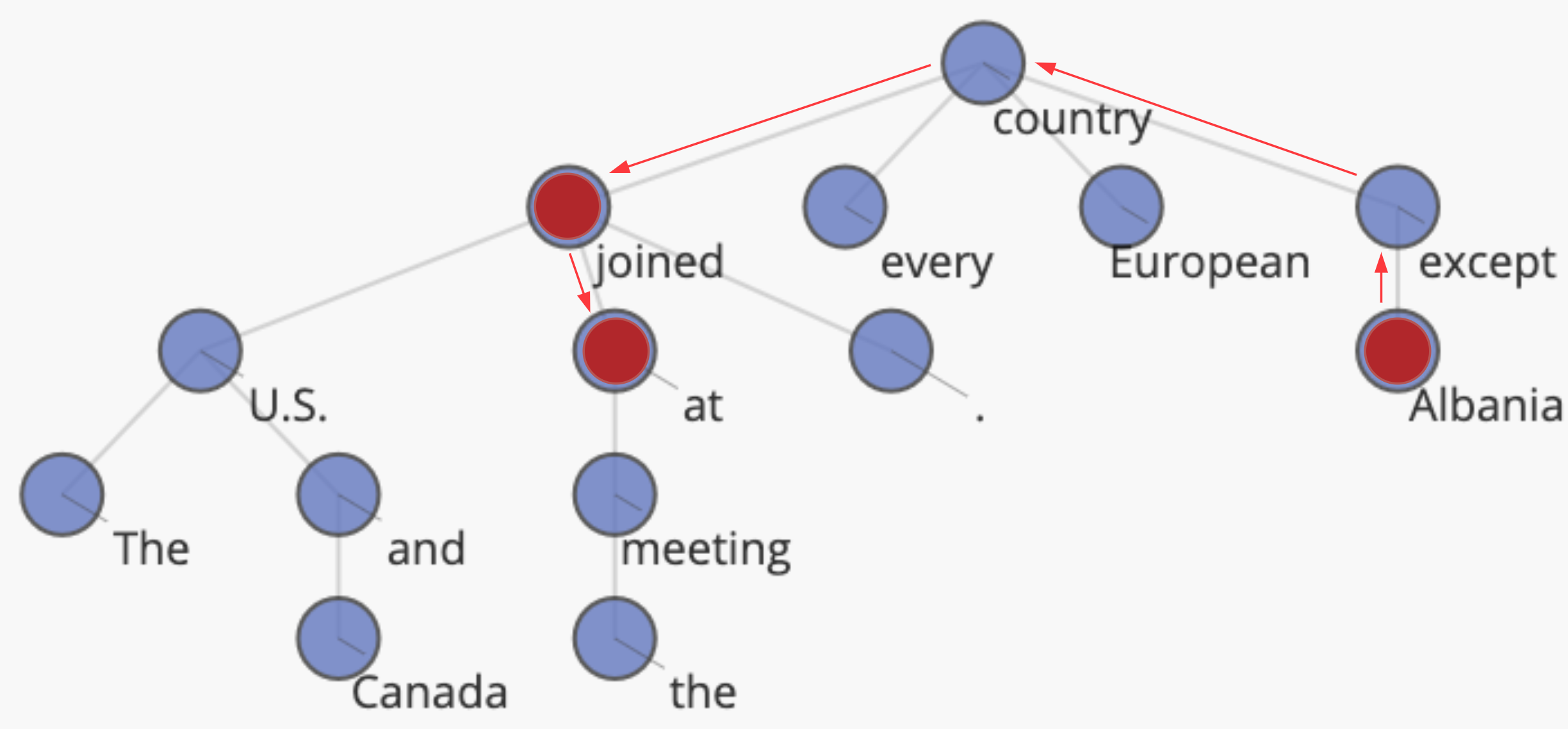
Figure 3: The dependency tree of the sample sentence. We highlight the path from the word Albania to its most attended words joined and at.

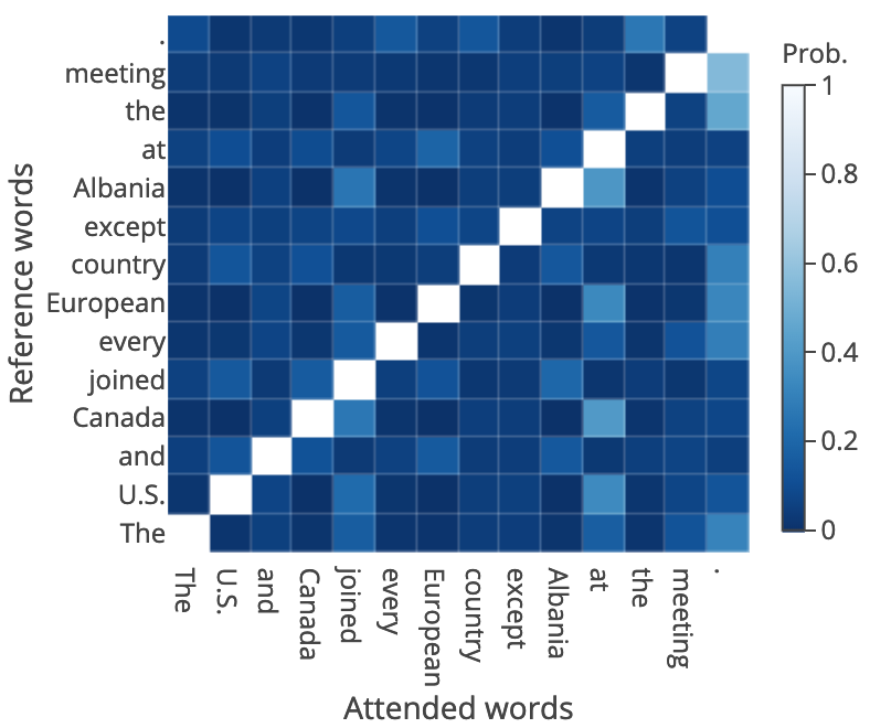
Figure 4: The relative attention matrix $A$, as described in Eq. 1, holds a probability distribution on every row. The main diagonal is excluded from all the probability distributions.

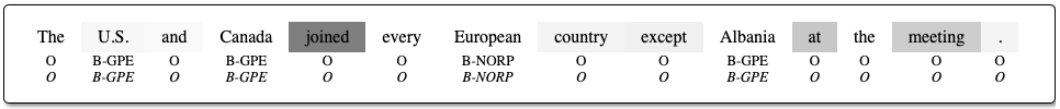
Figure 5: The visualization of global attention. The more highlighted the token is, the more probability mass it has. The labels and predictions (italics) appear below each word.

Relative attention. Figure 4 shows the relative attention matrix for the dependency tree in Figure 3. Each row of the matrix draws a probability distribution over the rest of the words (columns). By inspecting the matrix, it is easy to note that the words at and joined in the x-axis are the most relevant for Albania in the y-axis, whereas U.S., Canada, European, and Albania (x-axis) are the most important for joined (y-axis). This supports the idea that prioritizing words based on their relationships can provide different perspectives of the sentence at the word level. Additionally, when we inspect the models Blstm and Tlstm separately, we see different patterns captured in their attention matrices; for Blstm the relations are prioritized semantically (e.g., verbs are the most important parts and prepositions are hardly highlighted), whereas for Tlstm it is more syntactically (e.g., prepositions, verbs, punctuations are all relevant). Merging both techniques improves the results because they are complementary.

Global attention. Figure 5 shows the attended words once the relative attention matrix has extracted the prioritized relations. The figure shows a combination of both syntactic and semantic patterns. That is, while words like joined and meeting would be semantically expected, the model also focus on except, at, and the punctuation. Importantly, our model does not act as an entity spotter at this level. Instead, it relies on the syntactic structure of the sentence. Additionally, note that the word meeting was not too relevant in the relative attention matrix, but at the global perspective, it becomes important. This suggests that the attention mechanisms are complementary.

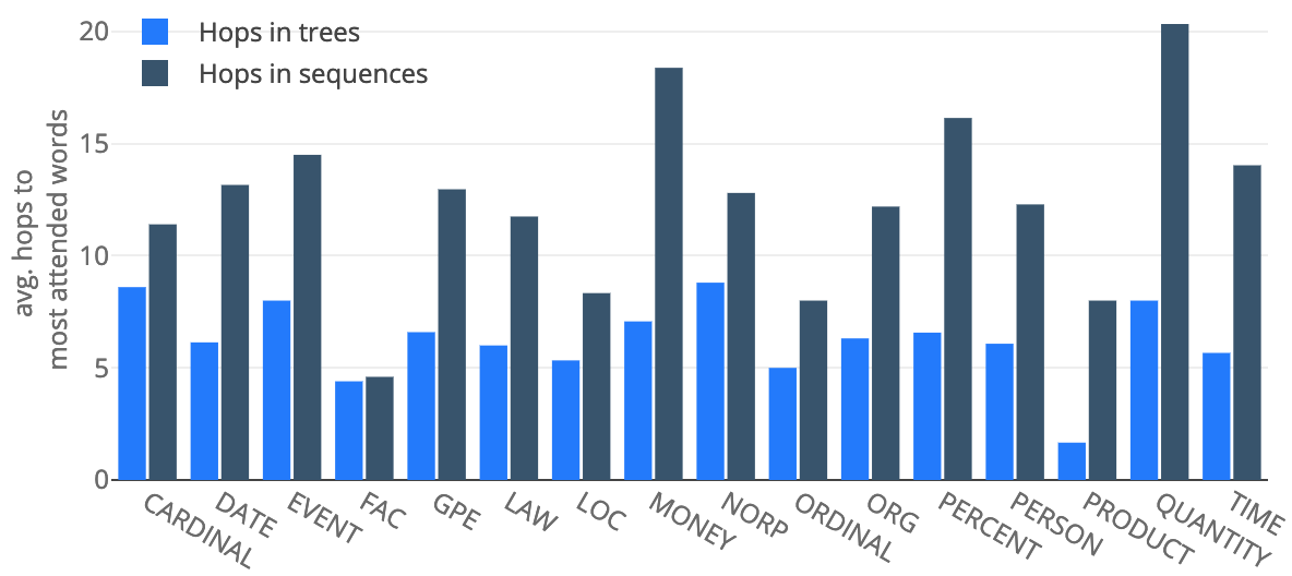
Figure 6: Average of hops to the most attended words in the validation set with respect to the entity tokens. For sequences, the hops are the number of tokens in between the entity and the most attended word. For trees, the hops are the number of nodes in the path that connects the entity and the most attended word.

Entity	POS	Coverage	Most Attended Words
PERSON	NN	31.53%	mr., correspondent, events, assistant, suit, case, ms., poll, a.m., consultant, president, express, officer, ignorance, cbs, wife, member, years, diet, menswear, life, relations, sunday, instance, season, network, school, woman, professor
	VB	15.88%	say, speak, come, go, write, begin, produce, need, tie, star, schedule, re-create, report, take, die, call, feature, love, continue, agree, know, pinch, consider, co-anchored, waive, brush, happen, issue, thank, welcome, slat, age, loot, resign, wrap, fall, chew, entomb, upset, allay, admire, place, strengthen
LOCATION	VB	28.42%	show, mellow, hold, direct, entitle, possess, continue, allow, travel, reach, begin, report, play, meet, carry, cause, miss, reduce, happen, mean, threaten, decide
	NN	23.50%	approaches, pollution, correspondent, temperatures, earthquake, u.s., meters, toepfer, run, re-enactment, behavior, mechanisms, breach, secrets, francisco, suspect, verdict, role, clue, analysis, thompson, space, story, zealand, violence, freedom, europe, front, glacier, conference, way, russia, death, cause, lake

Table 4: The most attended words for nouns that are labeled as PERSON or LOCATION. The table shows the attended POS tag per entity, its coverage, and the corresponding list of words.

Attended word distances. We also calculate the distance between the entities and its most attended words. That is, we take the attention matrix $A$, look for the rows whose tokens are labeled as entities, extract the most attended words, and calculate the number of hops between the entities and the extracted words for both the sentence sequence and the dependency trees. Figure 6 clearly shows that the most attended words by our model are closer when their layout is a tree instead of a sequence. This partially explains the better performance of the Tlstm_Word+PoS over the Blstm_Word+PoS, which also aligns with our claim that the long distance relations are potentially lost along the sentence when the words are treated as a plain sequence of tokens.

Entity correlations. We investigate whether the attended words with respect to the entity tokens follow any particular pattern. We conduct the study by controlling over the entity types and their corresponding POS tags. Specifically, we only consider the entity tokens whose POS tags are nouns (e.g., NN, NNS, NNP, or NNPS). Then, we extract the top three most attended words along with their POS tags from the SemEval 2010 validation set. In Table 4, we show the coverage of the most attended POS tags and their corresponding words for PERSON and LOCATION. For the type PERSON, the nouns president, assistant, and officer are roles that only people perform, which easily discriminate the type PERSON from any other entity type. In the case of its attended verbs, speak, love, and die are actions also performed by people (i.e., the entity is the subject of the sentence). For the type LOCATION, the verbs entitle, travel, and meet appear in cases where the location is the object of the sentence, and as such, these verbs disclose enough information to recognize that the entity is a place. Similarly, the nouns pollution, earthquake, and temperatures are commonly used to describe the state or events in a specific location. These findings are consistent with our initial intuition that specific words, along with their syntactic roles, can disclose important clues to recognize a given entity.

4.3 Error analysis

Dataset	Dep. Trees	F1	Affected F1
SemEval-10	Manual	86.49	83.18 (3.31$\downarrow$)
CoNLL-12	Converted	88.97	86.94 (2.03$\downarrow$)
ON 5.0 (BN)	Converted	89.22	86.92 (2.30$\downarrow$)

Table 5: Impact on the performance when the dependency trees are generated from scratch. F1 shows the score using dependency trees from either manual annotation or converted from parsing trees. Affected F1 provides the scores with tool-generated dependency trees.

Our model captures reasonably well the intended syntactic patterns, but the performance greatly relies on the quality of the dependency trees. We assess the impact of the dependency trees by evaluating the model using automatically generated trees from the Stanford CoreNLP tool Manning et al. (2014). We replace the trees in the validation set of the SemEval 2010 dataset, which originally has manually annotated dependency parses. Not surprisingly, the F1 score drops by 3.31 absolute points (see Table 5). We perform the same evaluation on OntoNotes 5.0 (BN) and CoNLL 2012. Similarly, the F1 score decreases by 2.30 and 2.03 points on each dataset, respectively. By further inspection of the trees generated from scratch, we find that they contain multiple roots mainly because of the multiple utterances that are transcribed from speech in the elaboration of these datasets. Multi-rooted trees affect the performance of the Tree-LSTM model because they prevent connecting information across the sentence. Additionally, Table 5 shows a smaller drop in performance on CoNLL 2012 and OntoNotes 5.0 (BN) compared to the drop on SemEval 2010. This is because the automatic conversions of the parsing trees do not have the same quality of the manual annotations in SemEval 2010 (e.g., multi-rooted sentences or erroneous connections between the nodes), and consequently the drop on SemEval 2010 tends to be bigger.

5 Conclusion

We propose a novel approach that combines sequential and recursive linguistic properties for NER. Our model uses syntactic and semantic features extracted from Tlstm and Blstm, respectively. Then, we feed this information into the relative and global attention mechanisms. The relative attention allows our model to exploit linguistic properties over the sentence with respect to every word, while the global attention combines those properties to balance semantic and syntactic patterns. We benchmark our model on four datasets and establish a new state of the art on two of them. By exploring the relationships among the entities and the most attended words, we find that the model learns to detect words that disclose information of the entity types based on their syntactic properties.

Appendix A Hyper-parameter tuning

We initialize the embedding matrices for part-of-speech tags and dependency relations using Xavier initialization Glorot and Bengio (2010). While these embedding matrices are learned from scratch, we use the pre-trained language model ELMo to represent words Peters et al. (2018). The size of the POS tag and dependency relation matrices are one fourth of the dimensions of the word vectors. We use the small version of ELMo in most of the experiments, which contains 256-dimensional word vectors. In this case, POS tag and dependency relation representations would be of 64 dimensions each.

We train all our models for 150 epochs using an initial learning rate of 5e-3 and a batch size of 16. The optimization of the models is conducted using Stochastic Gradient Descent (SGD) with momentum Sutskever et al. (2013). We modify the learning rate every epoch using cosine annealing and warm restarts with $t_{o}=10$ and a multiplicative factor of 2 Loshchilov and Hutter (2016). Besides adding $\ell_{2}$ regularization, we also prevent over-fitting by applying input variational dropout Gal and Ghahramani (2015) to every component in our model.

We consistently use gradient clipping among our experiments. We clip the norm of the gradient at 5.0 (Pascanu et al., 2012; Goodfellow et al., 2016)

$$\mathbf{g}\leftarrow\frac{\mathbf{g}\tau}{||\mathbf{g}||}~{}~{}\mathrm{if}~{}||\mathbf{g}||>\tau$$

To regularize the models, we use input variational dropout (Gal and Ghahramani, 2015) choosing drop probabilities between 0.1 and 0.5, being 0.3 the best. We apply an $\ell_{2}$ regularization with a $\lambda$ penalty of 1e-5.

Appendix B Datasets

B.1 CoNLL 2003 Dataset

The CoNLL 2003 dataset contains 4 entity labels: PERSON, LOCATION, ORGANIZATION and MISCELANEOUS. Table 6 shows statistics on the entity labels.

Statistics	Train	Dev	Test
Posts	14,041	3,250	3,453
Tokens	203,621	51,362	46,435
NE tokens	3,403	8,603	8,112
NE tokens (%)	1.67	16.74	17.46
Uniqueness (%)	26	40	41
Classes
Person	11,128	3,149	2,773
Location	8,297	2,094	1,925
Organization	10,025	2,092	2,496
Miscellaneous	4,593	1,268	918

Table 6: General statistics and class distribution of the CoNLL 2003 dataset.

B.2 SemEval 2010 Dataset

The SemEval 2010 Task 1 dataset is a subset of the OntoNotes 5.0 corpus that contains manually annotated dependency parses. This is the main dataset for our approach because of the manual annotations. The dataset contains 3,648 sentences for training, 741 for development and 1,141 for testing. The entity labels on this dataset are shown in Table 7.

Entities	Train	Dev	Test
ANIMAL	9	0	1
CARDINAL	532	93	207
DATE	1208	190	362
DISEASE	28	1	0
EVENT	26	6	6
FAC	72	19	16
GAME	4	1	0
GPE	1244	259	405
LANGUAGE	3	1	8
LAW	16	6	8
LOC	117	20	39
MONEY	296	57	54
NORP	588	110	205
ORDINAL	120	28	27
ORG	1351	381	560
PERCENT	332	27	48
PERSON	1282	331	372
PLANT	8	1	0
PRODUCT	74	14	57
QUANTITY	52	4	18
SUBSTANCE	154	15	31
TIME	109	33	50

Table 7: Statistics and distribution of the classes in the SemEval 2010 dataset.

B.3 CoNLL 2012 Dataset

The CoNLL 2012 uses the entire OntoNotes 5.0 corpus and proposes a standard split of the data. Table 8 shows the distribution of the labels after the split. Since the data comes from OntoNotes 5.0, the data contain parsing trees. Table 8 shows the distribution of the labels.

Entities	Train	Dev	Test
CARDINAL	10901	1720	1005
DATE	18791	3208	1787
EVENT	1009	179	85
FAC	1158	133	149
GPE	21938	3649	2546
LANGUAGE	355	35	22
LAW	459	65	44
LOC	2160	316	215
MONEY	5217	853	355
NORP	9341	1277	990
ORDINAL	2195	335	207
ORG	24163	3798	2002
PERCENT	3802	656	408
PERSON	22035	3163	2134
PRODUCT	992	214	90
QUANTITY	1240	190	153
TIME	1703	361	225
WORK OF ART	1279	202	169

Table 8: Statistics and distribution of the classes in the CoNLL 2012 dataset.

B.4 OntoNotes 5.0 Broadcast News Dataset

The broadcast news section of the OntoNotes 5.0 corpus is a small portion of the data. Table 9 shows the distribution of the labels.

Entities	Train	Dev	Test
CARDINAL	1639	155	196
DATE	2351	302	318
EVENT	111	14	24
FAC	275	24	36
GPE	4056	516	537
LANGUAGE	22	7	5
LAW	25	6	4
LOC	373	42	60
MONEY	177	14	20
NORP	2394	244	304
ORDINAL	366	53	47
ORG	2468	303	264
PERCENT	132	21	6
PERSON	4242	557	460
PRODUCT	327	35	43
QUANTITY	126	19	16
TIME	517	68	54
WORK OF ART	160	26	35

Table 9: General statistics and class distribution of the OntoNotes 5.0 Broadcast News section dataset.

References

- Aguilar et al. (2018) Gustavo Aguilar, Adrian Pastor López Monroy, Fabio González, and Thamar Solorio. 2018. Modeling noisiness to recognize named entities using multitask neural networks on social media. In Proceedings of the 2018 Conference of the North American Chapter of the Association for Computational Linguistics: Human Language Technologies, Volume 1 (Long Papers), pages 1401–1412, New Orleans, Louisiana. Association for Computational Linguistics.
- Akbik et al. (2018) Alan Akbik, Duncan Blythe, and Roland Vollgraf. 2018. Contextual string embeddings for sequence labeling. In Proceedings of the 27th International Conference on Computational Linguistics, pages 1638–1649. Association for Computational Linguistics.
- Ba et al. (2016) Jimmy Lei Ba, Jamie Ryan Kiros, and Geoffrey E Hinton. 2016. Layer normalization. arXiv preprint arXiv:1607.06450.
- Bahdanau et al. (2014) Dzmitry Bahdanau, Kyunghyun Cho, and Yoshua Bengio. 2014. Neural machine translation by jointly learning to align and translate. CoRR, abs/1409.0473.
- Chieu and Ng (2003) Hai Leong Chieu and Hwee Tou Ng. 2003. Named entity recognition with a maximum entropy approach. In Proceedings of the Seventh Conference on Natural Language Learning at HLT-NAACL 2003 - Volume 4, CONLL ’03, pages 160–163, Stroudsburg, PA, USA. Association for Computational Linguistics.
- Chiu and Nichols (2016) Jason Chiu and Eric Nichols. 2016. Named entity recognition with bidirectional lstm-cnns. Transactions of the Association for Computational Linguistics, 4:357–370.
- Devlin et al. (2018) Jacob Devlin, Ming-Wei Chang, Kenton Lee, and Kristina Toutanova. 2018. Bert: Pre-training of deep bidirectional transformers for language understanding. arXiv preprint arXiv:1810.04805.
- Feng et al. (2017) Yuntian Feng, Hongjun Zhang, Wenning Hao, and Gang Chen. 2017. Joint Extraction of Entities and Relations Using Reinforcement Learning and Deep Learning. Computational Intelligence and Neuroscience, Volume 2017, Article ID 7643065, 11 pages.
- Gal and Ghahramani (2015) Yarin Gal and Zoubin Ghahramani. 2015. Dropout as a Bayesian approximation: Representing model uncertainty in deep learning. arXiv:1506.02142.
- Glorot and Bengio (2010) Xavier Glorot and Yoshua Bengio. 2010. Understanding the difficulty of training deep feedforward neural networks. In Proceedings of the thirteenth international conference on artificial intelligence and statistics, pages 249–256.
- Goodfellow et al. (2016) Ian Goodfellow, Yoshua Bengio, and Aaron Courville. 2016. Deep Learning. MIT Press. http://www.deeplearningbook.org.
- He et al. (2015) Kaiming He, Xiangyu Zhang, Shaoqing Ren, and Jian Sun. 2015. Deep residual learning for image recognition. CoRR, abs/1512.03385.
- Hochreiter and Schmidhuber (1997) Sepp Hochreiter and Jürgen Schmidhuber. 1997. Long short-term memory. Neural Computation, 9(8):1735–1780.
- Howard and Ruder (2018) Jeremy Howard and Sebastian Ruder. 2018. Fine-tuned language models for text classification. CoRR, abs/1801.06146.
- Jie et al. (2017) Zhanming Jie, Aldrian Muis, and Wei Lu. 2017. Efficient dependency-guided named entity recognition. In Proceedings of the 2017 AAAI Conference on Artificial Intelligence.
- Jie Yang and Zhang (2018) Shuailong Liang Jie Yang and Yue Zhang. 2018. Design challenges and misconceptions in neural sequence labeling. In Proceedings of the 27th International Conference on Computational Linguistics (CONLING).
- Lample et al. (2016) Guillaume Lample, Miguel Ballesteros, Sandeep Subramanian, Kazuya Kawakami, and Chris Dyer. 2016. Neural architectures for named entity recognition. CoRR, abs/1603.01360.
- Limsopatham and Collier (2016) Nut Limsopatham and Nigel Collier. 2016. Bidirectional lstm for named entity recognition in twitter messages. In Proceedings of the 2nd Workshop on Noisy User-generated Text (WNUT), pages 145–152, Osaka, Japan. The COLING 2016 Organizing Committee.
- Liu et al. (2017) Liyuan Liu, Jingbo Shang, Frank F. Xu, Xiang Ren, Huan Gui, Jian Peng, and Jiawei Han. 2017. Empower sequence labeling with task-aware neural language model. CoRR, abs/1709.04109.
- Loshchilov and Hutter (2016) Ilya Loshchilov and Frank Hutter. 2016. SGDR: stochastic gradient descent with restarts. CoRR, abs/1608.03983.
- Ma and Hovy (2016) Xuezhe Ma and Eduard H. Hovy. 2016. End-to-end sequence labeling via bi-directional lstm-cnns-crf. CoRR, abs/1603.01354.
- Manning et al. (2014) Christopher D. Manning, Mihai Surdeanu, John Bauer, Jenny Finkel, Steven J. Bethard, and David McClosky. 2014. The Stanford CoreNLP natural language processing toolkit. In Association for Computational Linguistics (ACL) System Demonstrations, pages 55–60.
- Pascanu et al. (2012) Razvan Pascanu, Tomas Mikolov, and Yoshua Bengio. 2012. Understanding the exploding gradient problem. CoRR, abs/1211.5063.
- Peng and Dredze (2016a) Nanyun Peng and Mark Dredze. 2016a. Improving named entity recognition for chinese social media with word segmentation representation learning. In Proceedings of the 54th Annual Meeting of the Association for Computational Linguistics (Volume 2: Short Papers), pages 149–155, Berlin, Germany. Association for Computational Linguistics.
- Peng and Dredze (2016b) Nanyun Peng and Mark Dredze. 2016b. Learning word segmentation representations to improve named entity recognition for chinese social media. CoRR, abs/1603.00786.
- Peters et al. (2018) Matthew Peters, Mark Neumann, Mohit Iyyer, Matt Gardner, Christopher Clark, Kenton Lee, and Luke Zettlemoyer. 2018. Deep contextualized word representations. In Proceedings of the 2018 Conference of the North American Chapter of the Association for Computational Linguistics: Human Language Technologies, Volume 1 (Long Papers), pages 2227–2237, New Orleans, Louisiana. Association for Computational Linguistics.
- Pradhan et al. (2013) Sameer Pradhan, Alessandro Moschitti, Nianwen Xue, Hwee Tou Ng, Anders Björkelund, Olga Uryupina, Yuchen Zhang, and Zhi Zhong. 2013. Towards robust linguistic analysis using ontonotes. In Proceedings of the Seventeenth Conference on Computational Natural Language Learning, pages 143–152.
- Recasens et al. (2010) Marta Recasens, Lluís Màrquez, Emili Sapena, M Antònia Martí, Mariona Taulé, Véronique Hoste, Massimo Poesio, and Yannick Versley. 2010. Semeval-2010 task 1: Coreference resolution in multiple languages. In Proceedings of the 5th International Workshop on Semantic Evaluation, pages 1–8. Association for Computational Linguistics.
- Socher et al. (2012) Richard Socher, Brody Huval, Christopher D. Manning, and Andrew Y. Ng. 2012. Semantic compositionality through recursive matrix-vector spaces. In Proceedings of the 2012 Joint Conference on Empirical Methods in Natural Language Processing and Computational Natural Language Learning, EMNLP-CoNLL ’12, pages 1201–1211, Stroudsburg, PA, USA. Association for Computational Linguistics.
- Socher et al. (2011) Richard Socher, Cliff Chiung-Yu Lin, Andrew Y. Ng, and Christopher D. Manning. 2011. Parsing natural scenes and natural language with recursive neural networks. In Proceedings of the 28th International Conference on International Conference on Machine Learning, ICML’11, pages 129–136, USA. Omnipress.
- Sutskever et al. (2013) Ilya Sutskever, James Martens, George Dahl, and Geoffrey Hinton. 2013. On the importance of initialization and momentum in deep learning. In Proceedings of the 30th International Conference on Machine Learning, volume 28 of Proceedings of Machine Learning Research, pages 1139–1147, Atlanta, Georgia, USA. PMLR.
- Tai et al. (2015) Kai Sheng Tai, Richard Socher, and Christopher D. Manning. 2015. Improved semantic representations from tree-structured long short-term memory networks. In Proceedings of the 53rd Annual Meeting of the Association for Computational Linguistics and the 7th International Joint Conference on Natural Language Processing (Volume 1: Long Papers), pages 1556–1566, Beijing, China. Association for Computational Linguistics.
- Tjong Kim Sang and De Meulder (2003) Erik F. Tjong Kim Sang and Fien De Meulder. 2003. Introduction to the conll-2003 shared task: Language-independent named entity recognition. In Proceedings of the Seventh Conference on Natural Language Learning at HLT-NAACL 2003, pages 142–147.
- Vaswani et al. (2017) Ashish Vaswani, Noam Shazeer, Niki Parmar, Jakob Uszkoreit, Llion Jones, Aidan N. Gomez, Lukasz Kaiser, and Illia Polosukhin. 2017. Attention is all you need. CoRR, abs/1706.03762.
- Weischedel et al. (2013) Ralph Weischedel, Martha Palmer, Mitchell Marcus, Eduard Hovy, Sameer Pradhan, Lance Ramshaw, Nianwen Xue, Ann Taylor, Jeff Kaufman, Michelle Franchini, Mohammed El-Bachouti, Robert Belvin, and Ann Houston. 2013. OntoNotes Release 5.0. Philadelphia: Linguistic Data Consortium.
- Zhang et al. (2017) Yuhao Zhang, Victor Zhong, Danqi Chen, Gabor Angeli, and Christopher D. Manning. 2017. Position-aware attention and supervised data improve slot filling. In Proceedings of the 2017 Conference on Empirical Methods in Natural Language Processing, pages 35–45. Association for Computational Linguistics.