Bottomonia production and polarization in the NRQCD with $k_{T}$-factorization. I: $\Upsilon(3S)$ and $\chi_{b}(3P)$ mesons

¹Faculty of Physics, Lomonosov Moscow State University, 119991 Moscow, Russia
²Skobeltsyn Institute of Nuclear Physics, Lomonosov Moscow State University, 119991 Moscow, Russia
³Joint Institute for Nuclear Research, 141980 Dubna, Moscow Region, Russia

Abstract

The $\Upsilon(3S)$ production and polarization at high energies is studied in the framework of $k_{T}$-factorization approach. Our consideration is based on the non-relativistic QCD formalism for bound states formation and off-shell production amplitudes for hard partonic subprocesses. The transverse momentum dependent (TMD, or unintegrated) gluon densities in a proton were derived from the Ciafaloni-Catani-Fiorani-Marchesini (CCFM) evolution equation as well as from the Kimber-Martin-Ryskin (KMR) prescription. Treating the non-perturbative color octet transitions in terms of the multipole radiation theory and taking into account feed-down contributions from radiative $\chi_{b}(3P)$ decays, we extract the corresponding non-perturbative matrix elements for $\Upsilon(3S)$ and $\chi_{b}(3P)$ mesons from a combined fit to $\Upsilon(3S)$ transverse momenta distributions measured by the CMS and ATLAS Collaborations at the LHC energies $\sqrt{s}=7$ and $13$ TeV and central rapidities. Then we apply the extracted values to describe the CDF and LHCb data on $\Upsilon(3S)$ production and to investigate the polarization parameters $\lambda_{\theta}$, $\lambda_{\phi}$ and $\lambda_{\theta\phi}$, which determine the $\Upsilon(3S)$ spin density matrix. Our predictions have a good agreement with the currently available data within the theoretical and experimental uncertainties.

1 Introduction

Since it was first observed, the production of charmonia and bottomonia in hadronic collisions remains a subject of considerable theoretical and experimental studies. A theoretical framework for the description of heavy quarkonia production and decays is provided by the non-relativistic QCD (NRQCD) factorization[1, 2]. This formalism implies a separation of perturbatively calculated short-distance cross-sections for the production of $Q\bar{Q}$ pair in an intermediate Fock state ${}^{2S+1}L_{J}^{(a)}$ with spin $S$, orbital angular momentum $L$, total angular momentum $J$ and color representation $a$ from long-distance non-perturbative matrix elements (NMEs), which describe the transition of that intermediate $Q\bar{Q}$ state into a physical quarkonium via soft gluon radiation. The NMEs are assumed to be universal (process- and energy-independent), not dependent on the quarkonium momentum and obeying certain hierarchy in powers of the relative heavy quark velocity $v_{Q}\sim\log^{-1}m_{Q}/\Lambda_{\rm QCD}$ with $m_{Q}$ being the heavy quark mass. The color octet (CO) NMEs are not calculable within the theory and have to be only extracted from the data.

At present, the cross sections of prompt $S$- and $P$-wave charmonia production ($\psi^{\prime}$, $\chi_{c}$, $J/\psi$ and $\eta_{c}$) in $pp$ collisions are known at the next-to-leading order (NLO NRQCD)[3, 4, 5, 6, 7, 8, 9, 10, 11, 12, 13, 14, 15]. The dominant tree-level next-to-next-to-leading order (NNLO^∗) corrections to the color-singlet (CS) production mechanism have been calculated[16]. With properly adjusted values of NMEs, one can achieve a good agreement between the NLO NRQCD predictions and the experimental data on the $\psi^{\prime}$, $\chi_{c}$ and $J/\psi$ transverse momenta distributions[3, 4, 5, 6, 7, 8, 9, 10]. However, the extracted NMEs strongly depend on the minimal charmonia transverse momentum $p_{T}$ used in the fits and are almost incompatible with each other when obtained from fitting different data sets. Moreover, none of the fits can reasonably describe the $\psi^{\prime}$ and $J/\psi$ polarization data (the so-called ‘‘polarization puzzle’’). The fits involving low-$p_{T}$ data result in the conclusion that the $\psi^{\prime}$ and $J/\psi$ production at large transverse momenta is dominated by color-octet ${}^{3}S_{1}^{(8)}$ contributions with strong transverse polarization, that contradicts to the unpolarized production seen at the Tevatron and LHC. To obtain an unpolarized $\psi^{\prime}$ and $J/\psi$ mesons, it is necessary to assume that the production is dominated by the scalar ${}^{1}S_{0}^{(8)}$ intermediate state[4]. However, such assumption immediately contradicts recent $\eta_{c}$ production data since the respective $\eta_{c}$ and $J/\psi$ NMEs are related by the heavy quark spin symmetry (HQSS) principle[1, 2]. The HQSS requires that the $\eta_{c}$ and $J/\psi$ NMEs have to be determined from the simultaneous fit for the entire charmonia family, that turned out to be impossible in the NLO NRQCD (see also discussions[17, 18, 19]). The overall complicated situation is still far from understanding and has been even called ‘‘challenging’’[13].

A possible solution to the problem above has been proposed recently[20] in the framework of a model that interprets the soft final state gluon radiation (which transforms an unbound $Q\bar{Q}$ pair into a physical quarkonium state) as a series of color-electric dipole transitions. In this way the NMEs are represented in an explicit form inspired by the classical multipole radiation theory, that has dramatic consequences for the polarization of the final state mesons since the spin structure of the transition amplitudes is specified. The proposed approach leads to unpolarized or only weakly polarized charmonia either because of the cancellation between the ${}^{3}P_{1}^{(8)}$ and ${}^{3}P_{2}^{(8)}$ contributions or as a result of two successive color-electric $E1$ dipole transitions in the chain ${}^{3}S_{1}^{(8)}\rightarrow{}^{3}P_{J}^{(8)}\rightarrow{}^{3}S_{1}^{(1)}$ giving us the possibility to simultaneously solve the polarization puzzle for $J/\psi$ mesons and production puzzle for $\eta_{c}$ mesons[21, 22].

An alternative laboratory for understanding the physics of the hadronization of heavy quark pairs is provided by the $\Upsilon(nS)$ and $\chi_{b}(mP)$ production, which has been measured recently by the CMS[23, 24], ATLAS[25] and LHCb[26, 27] Collaborations at the LHC. Polarization of $\Upsilon(nS)$ mesons has been also investigated by the CMS[28] and LHCb[29] Collaborations. Due to heavier masses of bottomonia and smaller relative velocity $v_{b}$ of $b$ quarks in the bottomonium rest frame ($v_{b}\simeq 0.08$ against $v_{c}\simeq 0.23$), these processes could be even a more suitable case to apply the NRQCD factorization because of a more faster convergence of the double NRQCD expansion in strong coupling $\alpha_{s}$ and $v_{Q}$. The complete NLO NRQCD predictions for $\Upsilon(nS)$ and $\chi_{b}(mP)$ production in $pp$ and $p\bar{p}$ collisions were presented[30, 31, 32, 33, 34]. As it was shown, one can reasonably explain the LHC data, both on $\Upsilon(nS)$ or $\chi_{b}(mP)$ yield and $\Upsilon(nS)$ polarization, by taking into account latest measurements on the $\chi_{b}(mP)$ production. In particular, the polarization puzzle for $\Upsilon(3S)$ meson can be solved by considering the $\chi_{b}(3P)$ feed-down contributions[33, 34]. The latter have been observed recently by the LHCb Collaboration for the first time[35] and found to be rather significant (up to 40%).

However, it is important to investigate the $S$- and $P$-wave bottomonia production and polarization within the same framework which has been already successfully applied for charmonia[21, 22]. Here we start with a short series of papers dedicated to the $\Upsilon(nS)$ and $\chi_{b}(mP)$ production in $pp$ and $p\bar{p}$ collisions at the high energies, that continues line of our previous studies. In the present note we concentrate on the $\Upsilon(3S)$ production with a consistent treatment for large $\chi_{b}(3P)$ feed-down contribution. The $\Upsilon(1S),\Upsilon(2S),\chi_{b}(1P)$ and $\chi_{b}(2P)$ production requires a dedicated study which will be the subject of our forthcoming papers. To describe the perturbative production of the $b\bar{b}$ pair in the hard scattering subprocess we apply the $k_{T}$-factorization approach[36, 37]. This approach is based on the Balitsky-Fadin-Kuraev-Lipatov (BFKL)[38] or Ciafaloni-Catani-Fiorani-Marchesini (CCFM)[39] evolution equations, which resum large logarithmic terms proportional to $\ln s\sim\ln 1/x$, important at high energies (or, equivalently, at low longitudinal momentum fraction $x$ of proton carried by gluon). The $k_{T}$-factorization approach has certain technical advantages in the ease of including higher-order radiative corrections (namely, leading part of NLO + NNLO + $\dots$ terms corresponding to real gluon emissions in initial state) in the form of transverse momentum dependent (TMD, or unintegrated) gluon density function in a proton. To describe the non-perturbative transition of an unbound $b\bar{b}$ pair into physical bottomonia we employ the model[20]. We determine the NMEs for $\Upsilon(3S)$ and $\chi_{b}(3P)$ mesons from the $\Upsilon(3S)$ transverse momentum distributions measured by the CMS[23, 24] and ATLAS[25] Collaborations in the central rapidity region at $\sqrt{s}=7$ and $13$ TeV (where the $k_{T}$-factorization approach is expected to be mostly relevant) and from the relative production ratio $R^{\chi_{b}(3P)}_{\Upsilon(3S)}$ measured recently by the LHCb Collaboration at $\sqrt{s}=7$ and $8$ TeV[35]. Then, we examine the extracted NMEs on the Tevatron and LHC data taken by the CDF[41] and LHCb[26, 27] Collaborations and make predictions for polarization parameters $\lambda_{\theta}$, $\lambda_{\phi}$, $\lambda_{\theta\phi}$ (and frame-independent parameter $\tilde{\lambda}$), which determine the $\Upsilon(3S)$ spin density matrix and compare them to the currently available data[28, 42].

The outline of our paper is the following. In Section 2 we briefly recall the basic steps of our calculations. In Section 3 we perform a numerical fit and extract the NMEs from the LHC data. Then we check the compatibility of the extracted NMEs with the available data on $\Upsilon(3S)$ yeild and polarization. Our conclusions are collected in Section 4.

2 Theoretical framework

In the present note we follow the approach described in the earlier publications[43, 44, 45]. For the reader’s convenience, we briefly recall here main points of the theoretical scheme. Our consideration is based on the off-shell gluon-gluon fusion subprocesses that represent the true leading order (LO) in QCD:

$$g^{*}(k_{1})+g^{*}(k_{2})\rightarrow\Upsilon[{}^{3}S_{1}^{(1)}](p)+g(k),$$ (1)

$$g^{*}(k_{1})+g^{*}(k_{2})\rightarrow\Upsilon[{}^{1}S_{0}^{(8)},{}^{3}S_{1}^{(8)},{}^{3}P_{J}^{(8)}](p).$$ (2)

$$g^{*}(k_{1})+g^{*}(k_{2})\rightarrow\chi_{bJ}(p)[{}^{3}P_{J}^{(1)},{}^{3}S_{1}^{(8)}]\rightarrow\Upsilon(p_{1})+\gamma(p_{2}),$$ (3)

where $J=0,1$ or $2$ and the four-momenta of all particles are given in the parentheses. The color states taken into account are directly indicated. To obtain the production amplitudes for $b\bar{b}$ states with required quantum numbers from the ones for an unspecified $b\bar{b}$ state we use the appropriate projection operators. These operators for the spin-singlet and spin-triplet states read[46]:

$$\Pi_{0}=(\hat{p}_{\bar{b}}-m_{b})\gamma_{5}(\hat{p}_{b}+m_{b})/m^{3/2},$$ (4)

$$\Pi_{1}=(\hat{p}_{\bar{b}}-m_{b})\hat{\epsilon}(S_{z})(\hat{p}_{b}+m_{b})/m^{3/2},$$ (5)

where $m=2m_{b}$, $p_{b}=p/2+q$ and $p_{\bar{b}}=p/2-q$ are the four-momenta of the quark and anti-quark and $q$ is the four-momentum of quarks in the bound state, which is associated with the orbital angular momentum $L$. States with various projections of the spin momentum onto the $z$ axis are represented by the polarization four-vector $\hat{\epsilon}(S_{z})$. Then, to calculate off-shell production amplitudes (1) — (3), one has to integrate the product of the hard scattering amplitude $A(q)$ expanded in a series around $q=0$ and meson bound state wave function $\Psi^{(a)}(q)$ with respect to $q$:

$$A(q)\Psi^{(a)}(q)=A|_{q=0}\Psi^{(a)}(q)+q^{\alpha}(\partial A/\partial q^{\alpha})|_{q=0}\Psi^{(a)}(q)+\dots$$ (6)

A term-by-term integration of this series employs the identities[46]:

$$\int{{{d^{3}q}\over{(2\pi)^{3}}}\Psi^{(a)}(q)}={{1}\over{\sqrt{4\pi}}}\mathcal{R}^{(a)}(0),$$ (7)

$$\int{{{d^{3}q}\over{(2\pi)^{3}}}q^{\alpha}\Psi^{(a)}(q)}=-i\epsilon^{\alpha}(L_{z}){{\sqrt{3}}\over{\sqrt{4\pi}}}\mathcal{R^{\prime}}^{(a)}(0),$$ (8)

where $\mathcal{R}^{(a)}(x)$ is the radial wave function in the coordinate representation. The first term in (6) contributes to $S$-waves only and vanishes for $P$-wave. In contrast, the second term contributes only to $P$-waves and vanishes for $S$-wave. States with various projections of the orbital angular momentum onto the $z$ axis are represented by the polarization four-vector $\epsilon_{\mu}(L_{z})$. The corresponding NMEs are directly related to the wave functions $\mathcal{R}^{(a)}(x)$ and their derivatives[1, 2]:

$$\langle\mathcal{O}^{\cal Q}[{}^{2S+1}L_{J}^{(a)}]\rangle=2N_{c}(2J+1)|\mathcal{R}^{(a)}(0)|^{2}/4\pi,$$ (9)

$$\langle\mathcal{O}^{\cal Q}[{}^{2S+1}L_{J}^{(a)}]\rangle=6N_{c}(2J+1)|\mathcal{R^{\prime}}^{(a)}(0)|^{2}/4\pi$$ (10)

for $S$- and $P$-wave quarkonium $\cal Q$ respectively, where $N_{c}=3$. Additionally, the NMEs obey the multiplicity relations coming from HQSS at LO:

$$\langle\mathcal{O}^{\cal Q}[{}^{3}P_{J}^{(a)}]\rangle=(2J+1)\langle\mathcal{O}^{\cal Q}[{}^{3}P_{0}^{(a)}]\rangle.$$ (11)

A similar relation holds for color-octet ${}^{3}S_{1}^{(8)}$ states if $P$-wave quarkonia are considered. The color-singlet wave functions and their derivatives can be obtained from the potential model calculation[47, 48] or extracted from the measured quarkonia decay widths. Further evaluation of partonic amplitudes is straightforward and was done in our previous papers[43, 44, 45]. We only mention here that the summation over polarizations of the incoming off-shell gluons is performed according the BFKL prescription ${\sum{\epsilon^{\mu}\epsilon^{*\nu}}}={\bm{k}}_{T}^{\mu}{\bm{k}}_{T}^{\nu}/{\bm{k}}_{T}^{2}$, where ${\bm{k}}_{T}$ is the gluon transverse momentum orthogonal to the beam axis[36, 37]. The spin density matrix of the $S$-wave quarkonia is expressed in terms of the momenta $l_{1}$ and $l_{2}$ of the decay leptons and reads

$${\sum{\epsilon^{\mu}\epsilon^{*\nu}}}=3(l_{1}^{\mu}l_{2}^{\nu}+l_{1}^{\nu}l_{2}^{\mu}-{{m^{2}}\over{2}}g^{\mu\nu})/m^{2}.$$ (12)

This expression is equivalent to the standard expression $\sum{\epsilon^{\mu}\epsilon^{*\nu}}=-g^{\mu\nu}+p^{\mu}p^{\nu}/m^{2}$, but more suitable for determining the polarization observables. In all other respects the evaluation follows the standard QCD Feynman rules. The obtained results have been explicitly tested for gauge invariance by substituting the gluon momenta for corresponding polarization vectors. We have observed their gauge invariance even with off-shell initial gluons.

As it was done for the prompt charmonia production[21, 22], to describe the transition of an unbound octet $b\bar{b}$ quark pair to an observed singlet state we employ the mechanism proposed in[20]. In this approach, a soft gluon with a small energy $E\sim\Lambda_{\rm QCD}$ is emitted after the hard interaction is over, bringing away the unwanted color and changing other quantum numbers of the produced CO system. In the conventional NRQCD calculations the emitted final state gluons are regarded as carrying no energy-momentum, that is in obvious contradiction with confinement, which prohibits the emission of infinitely soft colored quanta. In reality, the $b\bar{b}$ system must undergo a kind of final state interaction, where the energy-momentum exchange must be larger than the typical confinement scale. Thus, having small energy of the emitted gluons gives us the confidence that we do not enter the confinement or perturbative domains. This is not the matter of only kinematical corrections since one cannot organize transition amplitudes with correct spin properties without some finite energy-momentum transfer. In our calculations such soft gluon emission is described by a classical multipole expansion, in which the electric dipole ($E1$) transition dominates[50]. Only a single $E1$ transition is needed to transform a $P$-wave state into an $S$-wave state and the structure of the respective ${{}^{3}P_{J}^{(8)}}\to{{}^{3}S_{1}^{(1)}}+g$ amplitudes is given by[50]:

$$A({}^{3}P_{0}^{(8)}\rightarrow\Upsilon+g)\sim k_{\mu}^{(g)}p^{\rm(CO)\mu}\epsilon_{\nu}^{(\Upsilon)}\epsilon^{(g)\nu},$$ (13)

$$A({}^{3}P_{1}^{(8)}\rightarrow\Upsilon+g)\sim e^{\mu\nu\alpha\beta}k_{\mu}^{(g)}\epsilon_{\nu}^{\rm(CO)}\epsilon_{\alpha}^{(\Upsilon)}\epsilon_{\beta}^{(g)},$$ (14)

$$A({}^{3}P_{2}^{(8)}\rightarrow\Upsilon+g)\sim p_{\mu}^{\rm(CO)}\epsilon_{\alpha\beta}^{\rm(CO)}\epsilon_{\alpha}^{(\Upsilon)}\left[k_{\mu}^{(g)}\epsilon_{\beta}^{(g)}-k_{\beta}^{(g)}\epsilon_{\mu}^{(g)}\right],$$ (15)

where $p^{\rm(CO)}_{\mu}$, $k^{(g)}_{\mu}$, $\epsilon^{(\Upsilon)}_{\mu}$, $\epsilon^{(g)}_{\mu}$, $\epsilon^{\rm(CO)}_{\mu}$ and $\epsilon^{\rm(CO)}_{\mu}$ are the momenta and polarization vectors of corresponding particles and $e^{\mu\nu\alpha\beta}$ is the fully antisymmetric Levi-Civita tensor. The transformation of color-octet $S$-wave state into the color-singlet $S$-wave state is treated as two successive $E1$ transitions ${}^{3}S_{1}^{(8)}\rightarrow{}^{3}P_{J}^{(8)}+g$, ${}^{3}P_{J}^{(8)}\rightarrow{}^{3}S_{1}^{(1)}+g$ proceeding via either of three intermediate ${}^{3}P_{J}^{(8)}$ states with $J=0,1,2$. For each of these transitions we apply the same expressions (13) — (15). Of course, all the expressions above are the same for gluons and photons (up to an overall color factor) and therefore can be used to calculate the polarization variables in radiative decays in feed-down process $\chi_{b}(3P)\rightarrow\Upsilon(3S)+\gamma$. Thus, the polarization of the outgoing $\Upsilon(3S)$ meson can then be calculated without any ambiguity.

The approach[20] contrasts to conventional NRQCD calculations which show that heavy quarkonia produced from high-$p_{T}$ gluons as ${}^{3}S_{1}^{(8)}$ states carry strong transverse polarization. With our completely different view on the heavy quarkonia depolarization mechanism, we finally arrive at a completely different set of the fitted NMEs (see Section 3). The squares of the matrix elements, as being too lengthy, are not presented here but implemented into the newly developed parton-level Monte-Carlo event generator pegasus[51].

The cross sections of $\Upsilon(3S)$ and $\chi_{b}(3P)$ production in the $k_{T}$-factorization approach are calculated as a convolution of the off-shell partonic cross sections and TMD gluon densities $f_{g}(x,\bm{k}^{2}_{T},\mu^{2})$ in a proton. The cross section for $2\rightarrow 2$ and $2\rightarrow 1$ subprocesses (1) — (3) can be written as:

$$\sigma=\int{{1}\over{8\pi(x_{1}x_{2}s)F}}f_{g}(x_{1},\bm{k}^{2}_{1T},\mu^{2})f_{g}(x_{2},\bm{k}^{2}_{2T},\mu^{2})\times\\ \times\overline{|A(g^{*}+g^{*}\rightarrow Q\bar{Q}+g)|^{2}}d\bm{p}^{2}_{T}d\bm{k}^{2}_{1T}d\bm{k}^{2}_{2T}dydy_{g}{{d\phi_{1}}\over{2\pi}}{{d\phi_{2}}\over{2\pi}},$$ (16)

$$\sigma=\int{{{2\pi}\over{x_{1}x_{2}sF}}f_{g}(x_{1},\bm{k}^{2}_{1T},\mu^{2})f_{g}(x_{2},\bm{k}^{2}_{2T},\mu^{2})\overline{|A(g^{*}+g^{*}\rightarrow Q\bar{Q})|^{2}}}d\bm{k}^{2}_{1T}d\bm{k}^{2}_{2T}dy{{d\phi_{1}}\over{2\pi}}{{d\phi_{2}}\over{2\pi}},$$ (17)

where $\phi_{1}$ and $\phi_{2}$ are the azimuthal angles of the initial off-shell gluons having the fractions of the momentum $x_{1}$ and $x_{2}$ and non-zero transverse momenta $\bm{k}^{2}_{1T}$ and $\bm{k}^{2}_{2T}$, $\bm{p}^{2}_{T}$ and $y$ are the transverse momentum and rapidity of produced mesons, $y_{g}$ is the rapidity of the outgoing gluon and $\sqrt{s}$ is the $pp$ center-of-mass energy. According to the general definition[52], the off-shell gluon flux factor $F$ is defined as $F=2\lambda^{1/2}(\hat{s},k_{1}^{2},k_{2}^{2})$, where $\hat{s}=(k_{1}+k_{2})^{2}$ and $\lambda(x,y,z)$ is the known kinematic function. Note that for $2\to 2$ subprocesses one can use the approximation $\lambda^{1/2}(\hat{s},k_{1}^{2},k_{2}^{2})\simeq\hat{s}\simeq x_{1}x_{2}s$. However, it is not suitable for the $2\to 1$ kinematics because the difference between $\hat{s}\simeq m^{2}_{\Upsilon}$ and $x_{1}x_{2}s=m_{\Upsilon}^{2}+p_{T}^{2}$ can make pronounced effect on the $p_{T}$ spectrum. This effect is specially discussed in Section 3.

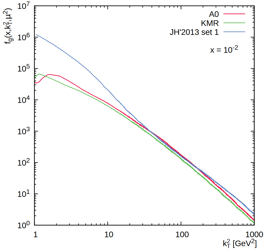
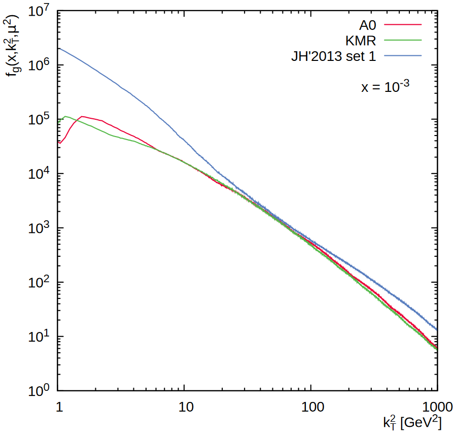
Figure 1: The TMD gluon densities in the proton calculated as a function of the gluon transverse momentum ${\mathbf{k}}_{T}^{2}$ at different longitudinal momentum fractions $x=10^{-2}$ (left panel) or $x=10^{-3}$ (right panel) and $\mu^{2}=10^{4}$ GeV².

In the present paper we have tested a few sets of the TMD gluon densities in a proton, namely, A0[53], JH’2013 set 1[54] and KMR[55] ones. First two of them were obtained from the numerical solutions of the CCFM gluon evolution equation. The CCFM equation provides a suitable tool since it converges to the BFKL equation in the region of small $x$ and to the DGLAP equation at large $x$ (see[39] for more details). The typical values of the variable $x$ probed in the considered processes are of order $x\sim(m_{\Upsilon}^{2}+p_{T}^{2})^{1/2}/\sqrt{s}$ at central rapidities, that corresponds to $x\sim 10^{-3}\,...\,10^{-2}$ in the kinematical conditions of the CMS and ATLAS experiments[23, 24, 25]. Thus, the CCFM evolution can be used in the whole $p_{T}$ range. The input parameters of these gluon distributions were determined from the best description of the precision DIS data on the proton structure functions $F_{2}(x,Q^{2})$. Additionally, we have used a set obtained with Kimber-Martin-Ryskin (KMR) prescription[55], which provides a method to evaluate the TMD parton densities from the conventional (collinear) ones. For the input, we have used recent LO NNPDF3.1 set[57]. The A0, JH’2013 and KMR gluon densities are shown in Fig. 1 as a function of ${\mathbf{k}}_{T}^{2}$ for different values of $x$ and $\mu^{2}$. One can observe a difference in the absolute normalization and shape between all these TMD gluon distributions. Below we discuss the corresponding phenomenological consequences.

The renormalization $\mu_{R}$ and factorization $\mu_{F}$ scales were set to $\mu_{R}^{2}=m_{\Upsilon}^{2}+p_{T}^{2}$ and $\mu_{F}^{2}=\hat{s}+{\mathbf{Q}}_{T}^{2}$ for CCFM-evolved gluon densities, where ${\mathbf{Q}}_{T}$ is the transverse momentum of the initial off-shell gluon pair. The choice of $\mu_{R}$ is a standard for bottomonia production, while the special choice of $\mu_{F}$ is connected with the CCFM evolution (see[53, 54]). In the KMR calculations, we used standard choice $\mu_{R}^{2}=\mu_{F}^{2}=m_{\Upsilon}^{2}+p_{T}^{2}$.

The parton level calculations were performed using the Monte-Carlo event generator pegasus[51].

3 Numerical results

As it was mentioned above, in the present paper we concentrate on the inclusive $\Upsilon(3S)$ and $\chi_{b}(3P)$ production, leaving other bottomonia states for forthcoming studies. Below we set the masses $m_{\Upsilon(3S)}=10.3552$ GeV, $m_{\chi_{b1}(3P)}=10.512$ GeV and $m_{\chi_{b2}(3P)}=10.522$ GeV [58] and adopt the usual non-relativistic approximation $m_{b}=m_{\cal Q}/2$ for the beauty quark mass, where $m_{\cal Q}$ is the mass of bottomonium $\cal Q$. We set the branching ratios $B(\Upsilon(3S)\rightarrow\mu^{+}\mu^{-})=0.0218$[58], $B(\chi_{b1}(3P)\rightarrow\Upsilon(3S)+\gamma)=0.1044$ and $B(\chi_{b2}(3P)\rightarrow\Upsilon(3S)+\gamma)=0.0611$[34]. Note that there are no experimental data for branching ratios of $\chi_{b}(3P)$, so the values above are the results of an assumption[34] that the total decay widths of $\chi_{b}(mP)$ are approximately independent on $m$. Following experimental analysis[35], we neglected the $\chi_{b0}(3P)$ contribution as it is almost zero. We use the one-loop formula for the coupling $\alpha_{s}$ with $n_{f}=4(5)$ quark flavours at $\Lambda_{\rm QCD}=250(167)$ MeV for A0 (KMR) gluon density and two-loop expression for $\alpha_{s}$ with $n_{f}=4$ and $\Lambda_{\rm QCD}=200$ MeV for JH’2013 set 1 gluon. As a commonly adopted choice, we set CS NMEs $\langle\mathcal{O}(\Upsilon[{}^{3}S_{1}^{(1)}])\rangle=3.54$ GeV³ and $\langle\mathcal{O}(\chi[{}^{3}P_{0}^{(1)}])\rangle=2.83$ GeV⁵. These values were obtained in the potential model calculations[47].

3.1 Fit of color octet NMEs

We have performed a global fit to the $\Upsilon(3S)$ production data at the LHC and determined the corresponding NMEs for both $\Upsilon(3S)$ and $\chi_{b}(3P)$ mesons. We have included in the fitting procedure the $\Upsilon(3S)$ transverse momentum distributions measured by the CMS[23, 24] and ATLAS[25] Collaborations at $\sqrt{s}=7$ and $13$ TeV and central rapidities, where our $k_{T}$-factorization calculations are most relevant due to essentially low-$x$ region probed. To determine NMEs for $\chi_{b}(3P)$ mesons, we also included into the fit the recent LHCb data[35] on the radiative $\chi_{b}(3P)\to\Upsilon(3S)+\gamma$ decays taken at $\sqrt{s}=7$ and $8$ TeV. We have excluded from our fit low $p_{T}$ region and consider only the data at $p_{T}>p_{T}^{\rm cut}=10$ GeV, where the NRQCD formalism is believed to be mostly reliable. As it was already mentioned above, the double NRQCD expansion in $\alpha_{s}$ and $v_{Q}$ is not good at low $p_{T}$, where a more accurate treatment of large logarithms $\sim\ln m_{\Upsilon}^{2}/p_{T}^{2}$ and other nonperturbative effects becomes necessary.

Before we proceed with the numerical fit, we would like to point out a few points. First of them is connected with the importance of proper definition of the off-shell flux factor for $2\to 1$ subprocesses (2) and (3). The definition of the flux, which is the velocity of the off-shell interacting partons, is not clear and can be disputable. As it was mentioned above, we use the ‘‘$\lambda^{1/2}$’’ prescription $F=2\lambda^{1/2}(\hat{s},k_{1}^{2},k_{2}^{2})$ in factorization formula (17). Our choice is based on the toy simulation[59] of $\chi_{c}$ meson production in $e^{+}e^{-}$ collisions. It was argued[59] that such definition leads to a good agreement of calculations based on Equivalent Photon Approximation and exact ${\cal O}(\alpha^{4})$ results. Contrary, the calculations performed with using conventional (collinear) $2\to 1$ flux treatment $\lambda^{1/2}(\hat{s},k_{1}^{2},k_{2}^{2})\simeq x_{1}x_{2}s$ did not reproduce the latter and therefore, in our opinion, seems to be rather doubtful.

Our calculation shows that the ‘‘$\lambda^{1/2}$’’ prescription results in different $p_{T}$ shapes of color-octet ${}^{1}S_{0}^{(8)}$ and ${}^{3}P_{J}^{(8)}$ contributions to the $\Upsilon(3S)$ production. Let us consider the ratio $R$ defined as

$$R={m_{\Upsilon(3S)}^{2}\sum\limits_{J=0}^{2}(2J+1)\,d\sigma[\Upsilon(3S),{}^{3}P_{J}^{(8)}]/dp_{T}\over d\sigma[\Upsilon(3S),{}^{1}S_{0}^{(8)}]/dp_{T}}$$ (18)

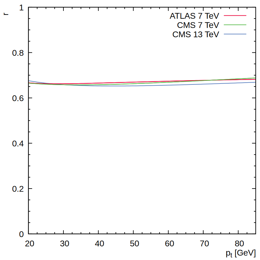
Figure 2: The production ratios $R$ (left panel) and $r$ (right panel) calculated as a function of $\Upsilon(3S)$ transverse momentum $p_{T}$ in the different kinematical regions.

as a function of $\Upsilon(3S)$ meson transverse momentum. While the calculations with collinear treatment of the flux factor $F$ show a flat behavior of this ratio in a wide $p_{T}$ region $10<p_{T}<100$ GeV (see Fig. 2, left panel) the calculations performed with using the ‘‘$\lambda^{1/2}$’’ prescription demonstrate the strong rise of the ratio $R$ with increasing $p_{T}$ giving us a possibility to separately extract the values of $\langle\mathcal{O}^{\Upsilon(3S)}[{}^{1}S_{0}^{(8)}]\rangle$ and $\langle\mathcal{O}^{\Upsilon(3S)}[{}^{3}P_{0}^{(8)}]\rangle$ from the experimental data. The latter turns out to be impossible when one inconsistently uses the collinear treatment of flux factor in the $k_{T}$-factorization calculations.

Our next point is connected with the correct treatment of feed-down contributions from the radiative decays of $\chi_{b}(3P)$ mesons, observed recently by the LHCb Collaboration[35]. We found that the $p_{T}$ shape of the direct $\Upsilon[^{3}S_{1}^{(8)}]$ and feed-down $\chi_{b}[^{3}S_{1}^{(8)}]$ contributions is almost the same in all kinematical regions probed by the LHC and Tevatron experiments. Thus, the ratio

$$r={\sum\limits_{J=0}^{2}(2J+1)\,B(\chi_{bJ}(3P)\to\Upsilon(3S)+\gamma)d\sigma[\chi_{bJ}(3P),{}^{3}S_{1}^{(8)}]/dp_{T}\over d\sigma[\Upsilon(3S),{}^{3}S_{1}^{(8)}]/dp_{T}}$$ (19)

can be well approximated by a constant for a wide $\Upsilon(3S)$ transverse momentum $p_{T}$ and rapidity $y$ ranges at different energies, as it is demonstrated in Fig. 2 (right panel). We estimate the mean-square average $r=0.654\pm 0.005$, which is practically independent on the TMD gluon density in a proton. Since up to now there are no experimental data on the $\chi_{b}(3P)$ transverse momentum distributions, we cannot separately determine the values of $\langle\mathcal{O}^{\Upsilon(3S)}[{}^{3}S_{1}^{(8)}]\rangle$ and $\langle\mathcal{O}^{\chi_{b0}(3P)}[{}^{3}S_{1}^{(8)}]\rangle$ from the available $\Upsilon(3S)$ data[23, 24, 25]. Instead, we introduce the linear combination

$$M_{r}=\langle\mathcal{O}^{\Upsilon(3S)}[{}^{3}S_{1}^{(8)}]\rangle+r\langle\mathcal{O}^{\chi_{b0}(3P)}[{}^{3}S_{1}^{(8)}]\rangle,$$ (20)

which can be extracted from the measured $\Upsilon(3S)$ transverse momentum distributions. Then we use recent LHCb data[35] on the fraction of $\Upsilon(3S)$ mesons originating from the $\chi_{b}(3P)$ radiative decays measured at $\sqrt{s}=7$ and $8$ TeV. To be precise, the LHCb Collaboration reported the ratio

$$R^{\chi_{b}(3P)}_{\Upsilon(3S)}=\sum\limits_{J=1}^{2}{\sigma(pp\rightarrow\chi_{bJ}(3P)+X)\over\sigma(pp\rightarrow\Upsilon(3S)+X)}\times B(\chi_{bJ}\to\Upsilon(3S)+\gamma),$$ (21)

where the possible contributions from $\chi_{b0}(3P)$ decays are neglected because of the small branching fraction. From the known $M_{r}$ and $R^{\chi_{b}(3P)}_{\Upsilon(3S)}$ values one can separately determine the $\langle\mathcal{O}^{\Upsilon(3S)}[{}^{3}S_{1}^{(8)}]\rangle$ and $\langle\mathcal{O}^{\chi_{b0}(3P)}[{}^{3}S_{1}^{(8)}]\rangle$, thus reconstructing full map of color octet NMEs for both $\Upsilon(3S)$ and $\chi_{b}(3P)$ mesons.

Using the strategy described above, we performed a numerical fit of $\Upsilon(3S)$ and $\chi_{b}(3P)$ NMEs. Nowhere we impose any kinematic restrictions but the experimental acceptance. The fitting procedure was separately done in each of the rapidity subdivisions (using the fitting algorithm as implemented in the commonly used gnuplot package[61]) under the requirement that all the NMEs are strictly positive. Then, the mean-square average of the fitted values was taken. The corresponding uncertainties are estimated in the conventional way using Student’s t-distribution at the confidence level $P=80$%. The results of our fits are collected in Table 1. For comparison, we also presented there the NMEs obtained in the conventional NLO NRQCD by other authors[33]. We have found that extracted values of $\langle\mathcal{O}^{\Upsilon(3S)}[{}^{1}S_{0}^{(8)}]\rangle$ are compatible with zero for all the TMD gluon densities. However, other color octet NMEs strongly depend on the latter, although JH’2013 set 1 and KMR gluons result in the more or less close values. The dependence of the fitted NMEs values on the TMD gluon densities reflects their different $x$ and ${\mathbf{k}}_{T}^{2}$ behavior, that is the consequence of different approaches to evaluate them. The corresponding $\chi^{2}/d.o.f.$ are listed in Table 2, where we additionally show their dependence on the $p_{T}^{\rm cut}$. As one can see, the $\chi^{2}/d.o.f.$ decreases when $p_{T}^{\rm cut}$ grows up and the best fit of the data is achieved with A0 gluon. We note that the returned relatively large (but still reasonable) $\chi^{2}/d.o.f.$ values are connected with the recent precision CMS data[24] included into the fit. So, as an exercise, we have excluded these data and repeated the fit procedure using the ATLAS data[25] only. In this way, the $\chi^{2}/d.o.f.\sim 1$ was obtained for all the considered TMD gluon densities.

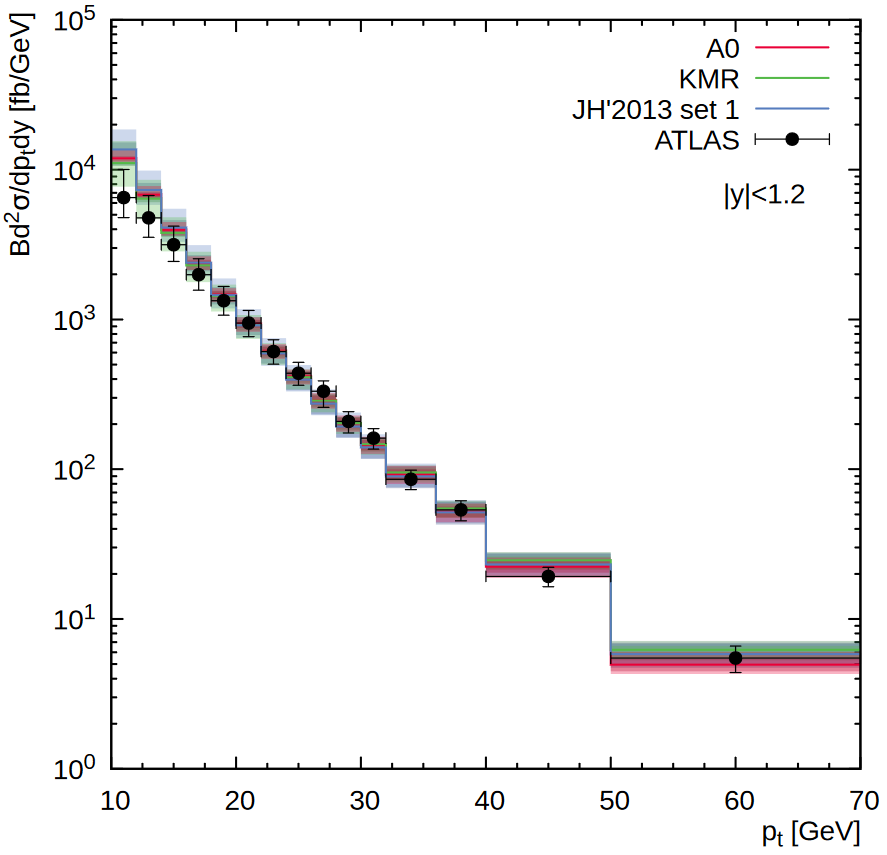
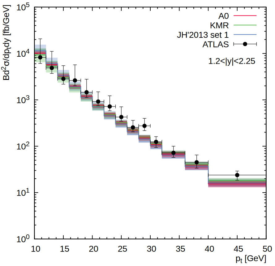
Figure 3: Transverse momentum distribution of inclusive $\Upsilon(3S)$ production calculated at $\sqrt{s}=7$ TeV in the different rapidity regions. The red, green and blue histograms correspond to the predictions obtained with A0, KMR and JH’2013 set 1 gluon densities. Shaded bands represent the total uncertainties of our calculations, as it is described in text. The experimental data are from ATLAS[25].

All the data used in the fits are compared with our predictions in Figs. 3 — 5. Note that the data at $p_{T}>p_{T}^{\rm cut}=10$ GeV are only shown. The shaded areas represent the theoretical uncertainties of our calculations, which include the scale uncertainties, uncertainties coming from the NME fitting procedure and uncertainties connected with the choice of the intermediate color-octet mass, added in quadrature. To estimate the scale uncertainties the standard variations in the scale $\mu_{R}\to 2\mu_{R}$ or $\mu_{R}\to\mu_{R}/2$ were introduced through replacing the gluon densities A0 and JH’2013 set 1 with A0$+$ and JH’2013 set 1$+$, or with A0$-$ and JH’2013 set 1$-$. This was done to preserve the intrinsic correspondence between the TMD set and the scale used in the evolution equation (see[53, 54]). To estimate the uncertainties connected with the intermediate color-octet mass we have varied amount of energy $E$ emitted in the course of transition of an unbound color octet $b\bar{b}$ pair into the observed bottomonium by a factor of $2$ around its default value $E=\Lambda_{\rm QCD}$. We find that the main effect here is only in changing the overall normalization with almost no changes in the shape of the $p_{T}$ spectrum (see also[62]). These uncertainties are about of $20$% and therefore comparable with the scale uncertainties. One can see that we have achieved a reasonably good description of the CMS[23, 24] and ATLAS[25] data in the whole $p_{T}$ range within the experimental and theoretical uncertainties for the $\Upsilon(3S)$ transverse momentum distributions. The ratio $R^{\chi_{b}(3P)}_{\Upsilon(3S)}$ measured by the LHCb Collaboration[35] is well described also. At large $p_{T}$, the JH’2013 set 1 and KMR gluons tend to overestimate the latest CMS data[24] taken at $\sqrt{s}=13$ TeV, but agree well with other measurements. This result shows a dependence of our predictions on the TMD gluon densities in certain kinematical regions.

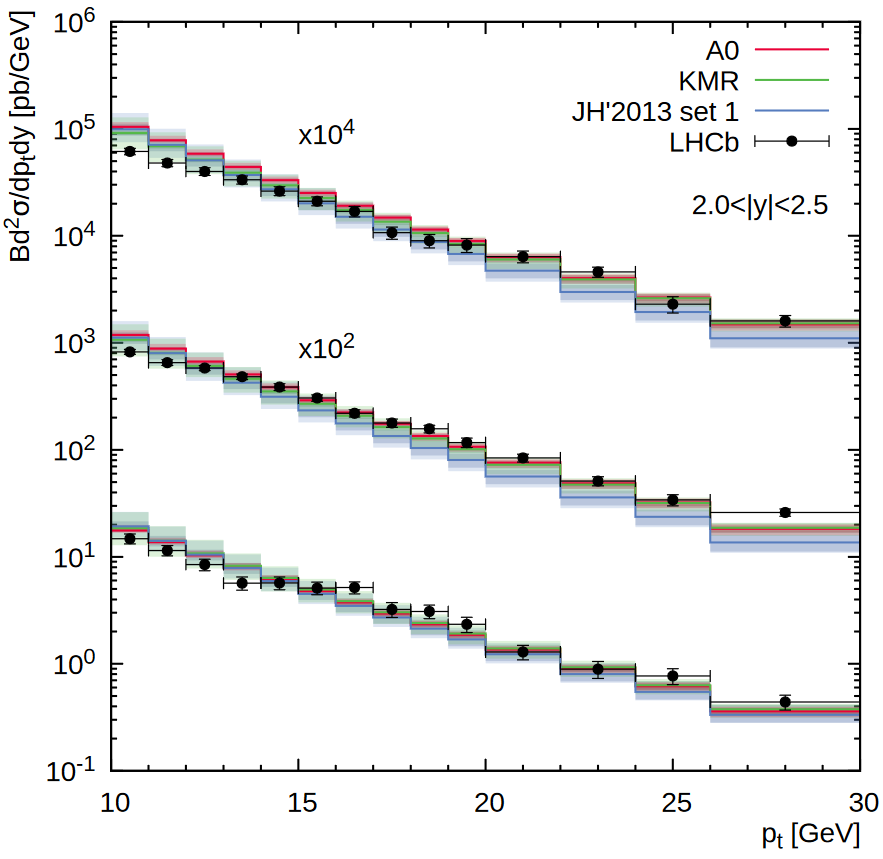
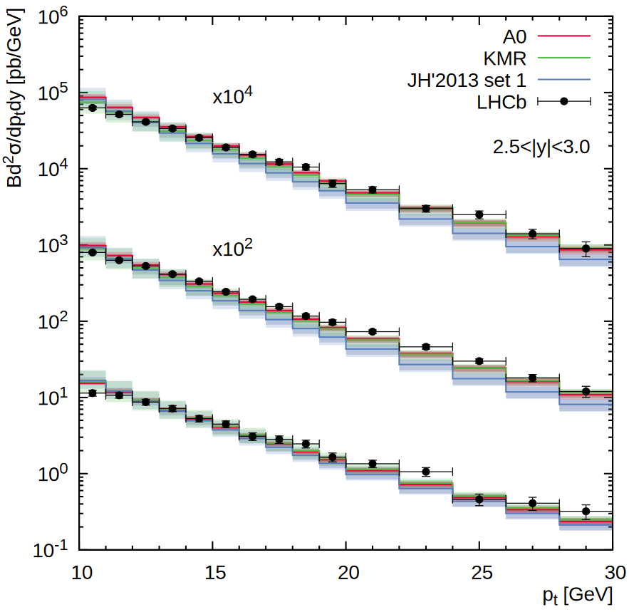
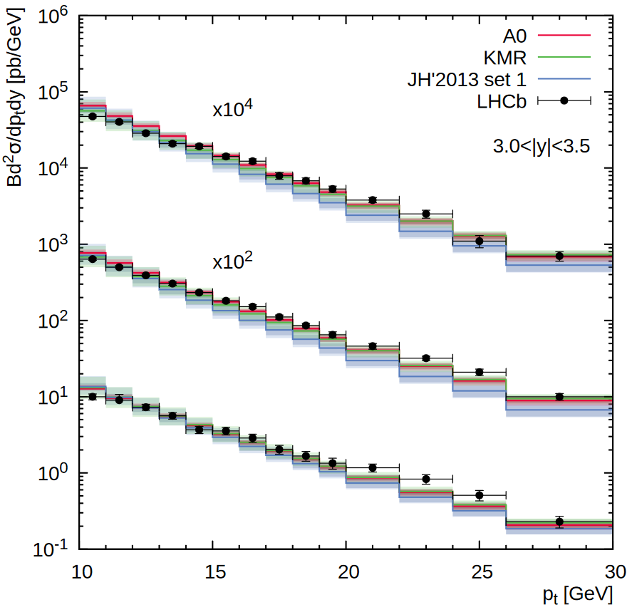
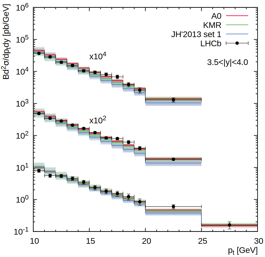
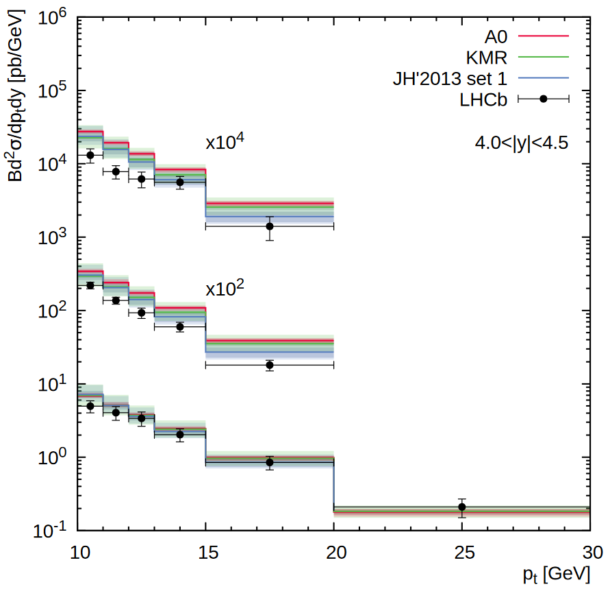
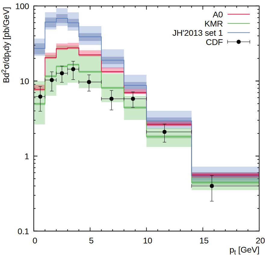
Figure 6: Transverse momentum distribution of inclusive $\Upsilon(3S)$ production calculated at $\sqrt{s}=1.8$, $7$, $8$ and $13$ TeV in the different rapidity regions. Notation of all histograms is the same as in Fig. 3. The experimental data are from CDF[41] and LHCb[26, 27].

With obtained NMEs for $\Upsilon(3S)$ and $\chi_{b}(3P)$ mesons, we achieved reasonably good description (of course, at $p_{T}>p_{T}^{\rm cut}$) of the earlier CDF data[41] taken at the $\sqrt{s}=1.8$ TeV and recent data[26, 27] taken by the LHCb Collaboration at $\sqrt{s}=7$, $8$ and $13$ TeV and forward rapidities, see Fig. 6. We find that the KMR gluon distribution is able to describe well the CDF data even at low $p_{T}$ region, $p_{T}<10$ GeV. Some discrepancy between the LHCb data and our predictions observed in very forward region $4<y<4.5$ at $\sqrt{s}=7$ TeV can be easily understood since here one can probe the essentially large-$x$ region, there the $k_{T}$-factorization becomes less applicable.

The consequence of our fit for $\Upsilon(3S)$ polarization is discussed in the next Section.

3.2 $\Upsilon(3S)$ polarization

As it is well known, the polarization of any vector meson can be described with three parameters $\lambda_{\theta}$, $\lambda_{\phi}$ and $\lambda_{\theta\phi}$, which determine the spin density matrix of a meson decaying into a lepton pair and can be measured experimentally. The double differential angular distribution of the decay leptons can be written as[63]:

$${{d\sigma}\over{d\cos\theta^{*}d\phi^{*}}}\sim{{1}\over{3+\lambda_{\theta}}}(1+\lambda_{\theta}\cos^{2}\theta^{*}+\lambda_{\phi}\sin^{2}\theta^{*}\cos 2\phi^{*}+\lambda_{\theta\phi}\sin 2\theta^{*}\cos\phi^{*}),$$ (22)

where $\theta^{*}$ and $\phi^{*}$ are the polar and azimuthal angles of the decay lepton measured in the meson rest frame. The case of $(\lambda_{\theta}$, $\lambda_{\phi}$, $\lambda_{\theta\phi})=(0,0,0)$ corresponds to unpolarized state, while $(\lambda_{\theta}$, $\lambda_{\phi}$, $\lambda_{\theta\phi})=(1,0,0)$ and $(\lambda_{\theta}$, $\lambda_{\phi}$, $\lambda_{\theta\phi})=(-1,0,0)$ refer to fully transverse and fully longitudinal polarizations.

The CMS Collaboration has measured all of these parameters as functions of $\Upsilon(3S)$ transverse momentum in three complementary frames: the Collins-Soper, helicity and perpendicular helicity ones at $\sqrt{s}=7$ TeV[28]. The CDF Collaboration also measured these parameters in the helicity frame at $\sqrt{s}=1.96$ TeV[42]. In the Collins-Soper frame the polarization axis $z$ bisects the two beam directions whereas the polarization axis in the helicity frame coincides with the $\Upsilon(3S)$ direction in the laboratory frame. In the perpendicular helicity frame the $z$ axis is orthogonal to that in the Collins-Soper frame and lies in the plane spanned by the two beam ($P_{1}$ and $P_{2}$) momenta. In all cases, the $y$ axis is taken to be in the direction of the vector product of the two beam directions in the $\Upsilon(3S)$ rest frame, $\vec{P}_{1}\times\vec{P}_{2}$ and $\vec{P}_{2}\times\vec{P}_{1}$ for positive and negative rapidities, respectively. Additionally, the frame-independent parameter $\tilde{\lambda}=(\lambda_{\theta}+3\lambda_{\phi})/(1-\lambda_{\phi})$ has been studied[28, 42]. Below we estimate the polarization parameters $\lambda_{\theta}$, $\lambda_{\phi}$, $\lambda_{\theta\phi}$ and $\tilde{\lambda}$ for the CMS and CDF conditions. As it was done earlier[22, 43, 44, 45], our calculation generally follows the experimental procedure. We collect the simulated events in the kinematical region defined by the CMS and CDF experiments, generate the decay lepton angular distributions according to the production and decay matrix elements and then apply a three-parametric fit based on (22). Of course, we took into account the polarization of $\Upsilon(3S)$ mesons originated from radiative $\chi_{b}(3P)$ decays, that is in full agreement with the experimental setup.

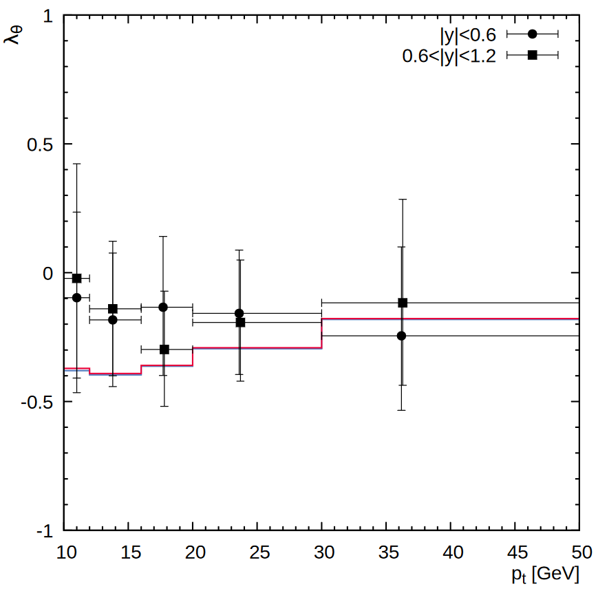
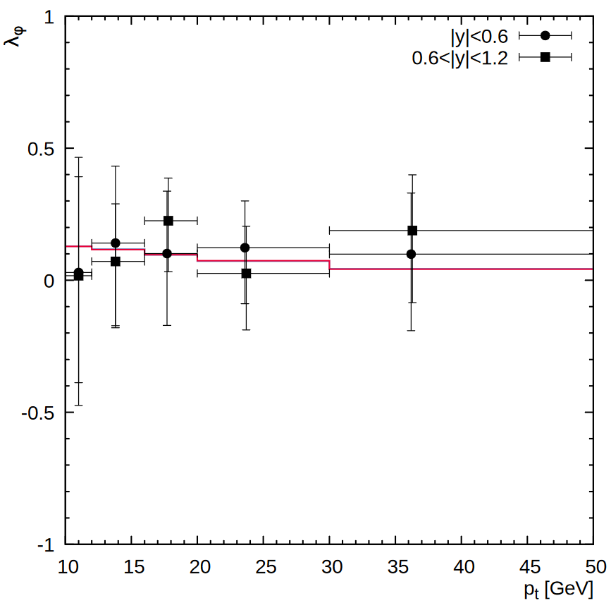
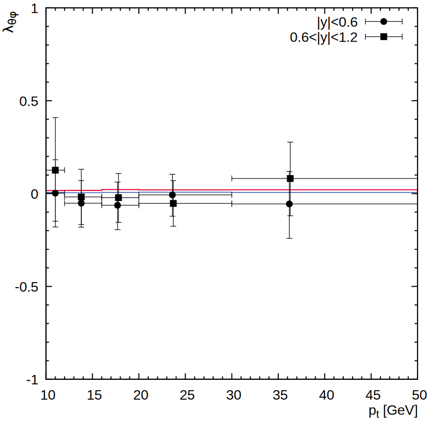
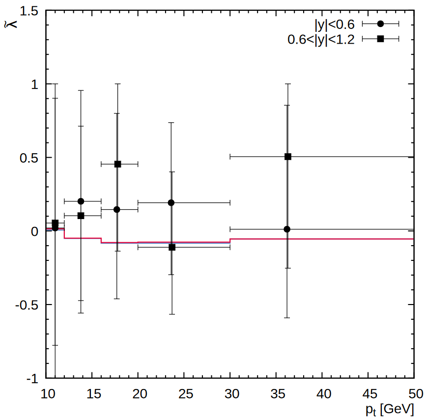
Figure 7: The polarization parameters $\lambda_{\theta}$, $\lambda_{\phi}$, $\lambda_{\theta\phi}$ and $\tilde{\lambda}$ of $\Upsilon(3S)$ mesons calculated in the CS frame as function of its transverse momentum at $\sqrt{s}=7$ TeV. The A0 gluon density is used. The blue and red histograms correspond to the predictions obtained at $|y|<0.6$ and $0.6<|y|<1.2$, respectively. The experimental data are from CMS[28].

Our results are presented in Figs. 7 — 10. These calculations were done using the A0 gluon density which provides the best description of the measured $\Upsilon(3S)$ transverse momenta distributions. The obtained predictions for the $\Upsilon(3S)$ polarization parameters have a reasonable agreement with the CMS and CDF data. In all the kinematical regions we find only weak or zero polarization, which coincides with the measurements within the uncertainties. These predictions are practically independent of the $\Upsilon(3S)$ rapidity. The absence of strong polarization is not connected with parameter tuning, but seems to be a natural and rather general feature of the scenario[20]. Thus, one can conclude that treating the soft gluon emissions within the NRQCD as a series of color-electric dipole transitions does not contradicts the available Tevatron and LHC data on the $\Upsilon(3S)$ production. The same conclusion was done for charmonia family[21, 22].

Finally, we would like to note that the qualitative predictions for the $\lambda_{\theta}$, $\lambda_{\phi}$, $\lambda_{\theta\phi}$ and $\tilde{\lambda}$ are stable with respect to variations in the model parameters. In fact, there is practically no dependence on the strong coupling constant and TMD gluon densities, i.e. two of important sources of theoretical uncertainties cancel out. So, the proposed way, in our opinion, can provide an easy and natural solution to the quarkonia production and polarization puzzle.

4 Conclusion

We have considered the $\Upsilon(3S)$ production at the Tevatron and LHC in the framework of $k_{T}$-factorization approach. Our consideration was based on the off-shell production amplitudes for hard partonic subprocesses (including both color-singlet and color-octet contributions), NRQCD formalism for the formation of bound states and TMD gluon densities in a proton (derived from the CCFM evolution equation and KMR scheme as well). Treating the nonperturbative color octet transitions in terms of multipole radiation theory and taking into account feed-down contributions from the radiative $\chi_{b}(3P)$ decays, we extracted $\Upsilon(3S)$ and $\chi_{b}(3P)$ NMEs in a fit to $\Upsilon(3S)$ transverse momentum distributions measured by the CMS and ATLAS Collaborations at $\sqrt{s}=7$ and $13$ TeV. We have inspected the extracted NMEs with the available Tevatron and LHC data taken in different kinematical regions and demostrated that these NMEs do not contradict the data. We found that the best description is achieved with the CCFM-evolved A0 gluon density, although the KMR one is able to describe the data even at low transverse momenta. Then we estimated polarization parameters $\lambda_{\theta}$, $\lambda_{\phi}$, $\lambda_{\theta\phi}$ and frame-independent parameter $\tilde{\lambda}$ which determine the $\Upsilon(3S)$ spin density matrix. We show that treating the soft gluon emission as a series of explicit color-electric dipole transitions within the NRQCD leads to unpolarized $\Upsilon(3S)$ production at moderate and large transverse momenta, that is in agreement with the Tevatron and LHC data.

	A0	JH’2013 set 1	KMR	NLO NRQCD[33]
$\langle\mathcal{O}^{\Upsilon(3S)}[{}^{3}S_{1}^{(1)}]\rangle$/GeV3	$3.54$	$3.54$	$3.54$	$3.54$
$\langle\mathcal{O}^{\Upsilon(3S)}[{}^{1}S_{0}^{(8)}]\rangle$/GeV3	$0.0$	$0.0$	$0.0$	$-0.0107\pm 0.0107$
$\langle\mathcal{O}^{\Upsilon(3S)}[{}^{3}S_{1}^{(8)}]\rangle$/GeV3	$0.018\pm 0.001$	$0.007\pm 0.002$	$0.006\pm 0.001$	$0.0271\pm 0.0013$
$\langle\mathcal{O}^{\Upsilon(3S)}[{}^{3}P_{0}^{(8)}]\rangle$/GeV5	$0.0$	$0.09\pm 0.03$	$0.073\pm 0.006$	$0.0039\pm 0.0023$
$\langle\mathcal{O}^{\chi_{b0}(3P)}[{}^{3}P_{0}^{(1)}]\rangle$/GeV5	$2.83$	$2.83$	$2.83$	$2.83$
$\langle\mathcal{O}^{\chi_{b0}(3P)}[{}^{3}S_{1}^{(8)}]\rangle$/GeV3	$0.016\pm 0.003$	$0.009\pm 0.001$	$0.005\pm 0.001$	—

Table 1: The NMEs for $\Upsilon(3S)$ and $\chi_{b}(3P)$ mesons as determined from our fit at $p_{T}^{\rm cut}=10$ GeV. The NMEs obtained in the NLO NRQCD[33] are shown for comparison.

	$p_{T}^{\rm cut}=10$ GeV	$p_{T}^{\rm cut}=12$ GeV	$p_{T}^{\rm cut}=15$ GeV	$p_{T}^{\rm cut}=17$ GeV
A0	$2.35$	$1.99$	$1.79$	$1.72$
JH’2013 set 1	$4.22$	$3.59$	$3.28$	$3.21$
KMR	$2.59$	$2.43$	$2.38$	$2.37$

Table 2: The dependence of the $\chi^{2}/d.o.f.$ achieved in the fit procedure on the choice of $p_{T}^{\rm cut}$.

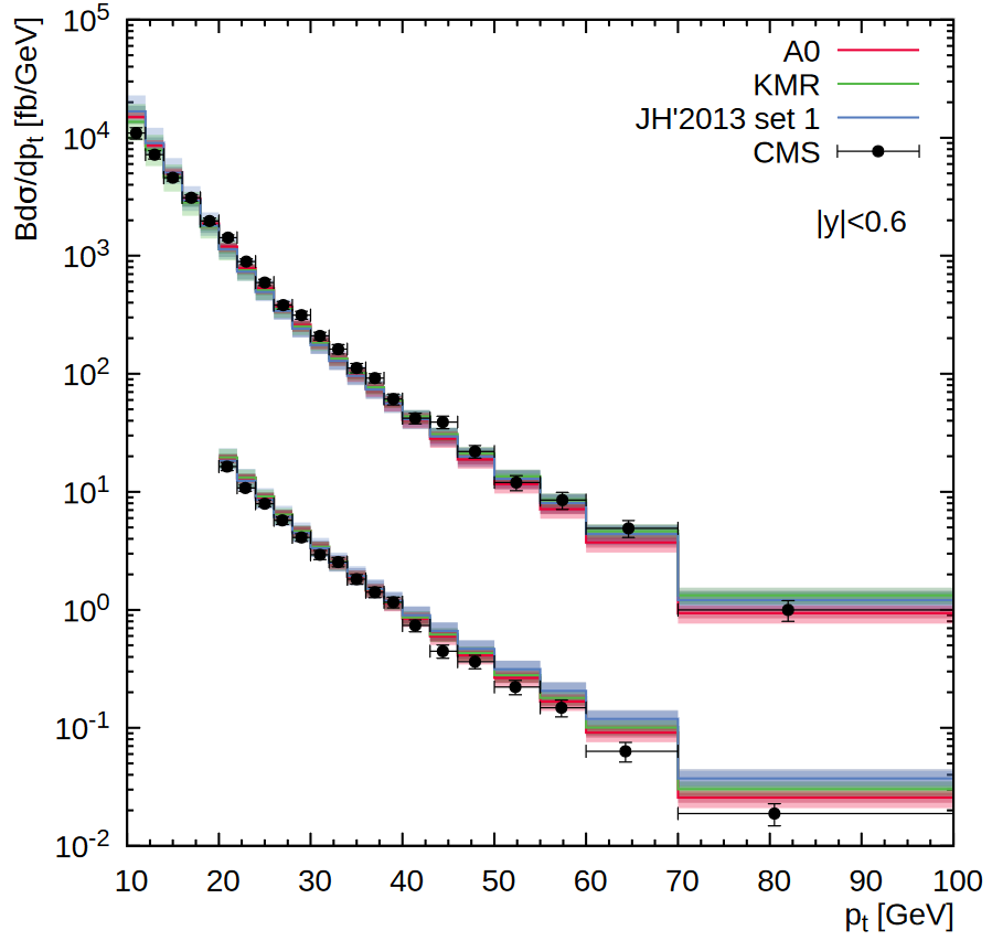
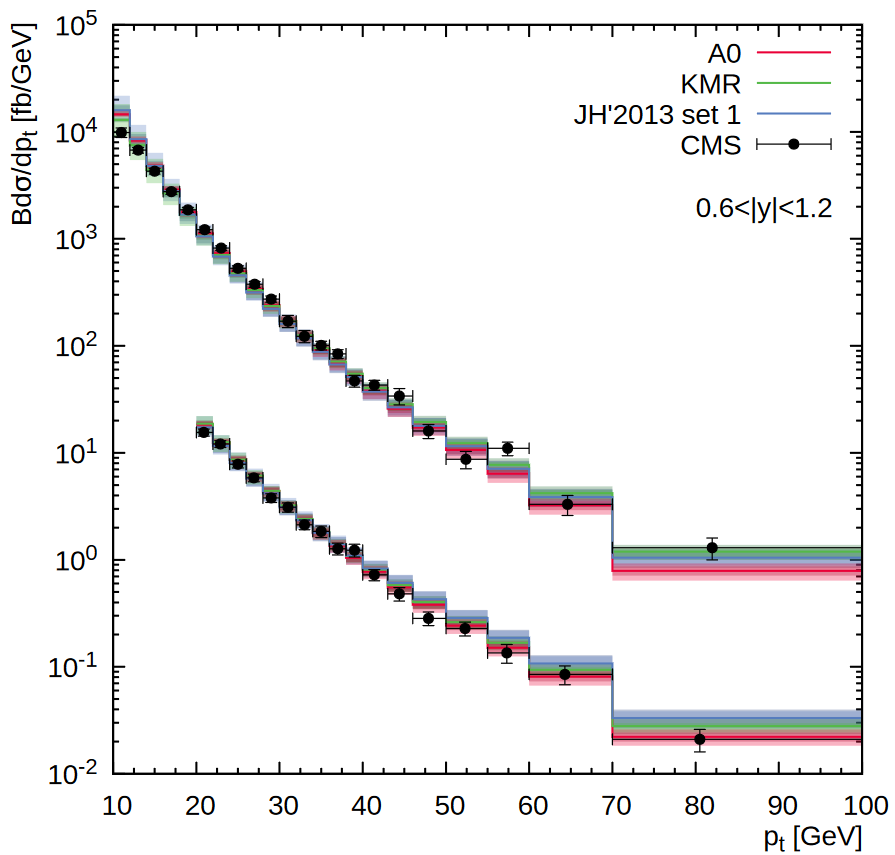
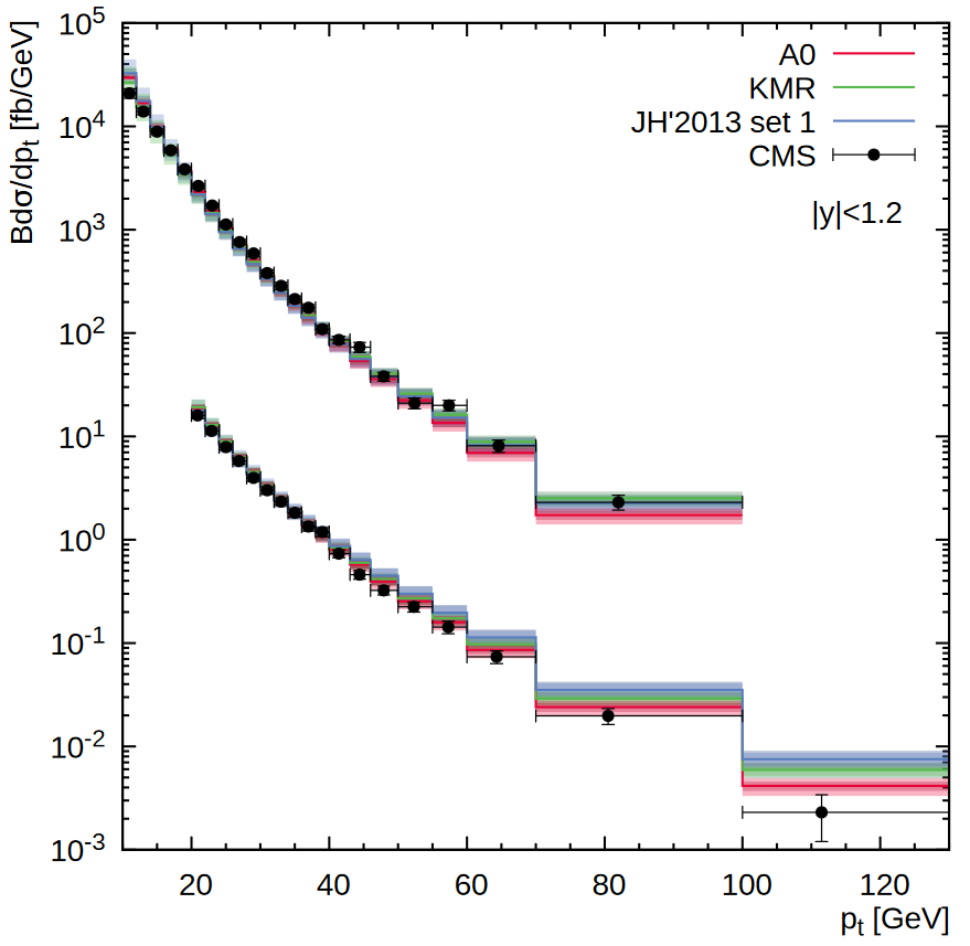
Figure 4: Transverse momentum distribution of inclusive $\Upsilon(3S)$ production calculated at $\sqrt{s}=7$ TeV (upper histograms) and $\sqrt{s}=13$ TeV (lower histograms, divided by $100$) in the different rapidity regions. Notation of all histograms is the same as in Fig. 3. The experimental data are from CMS[23, 24].

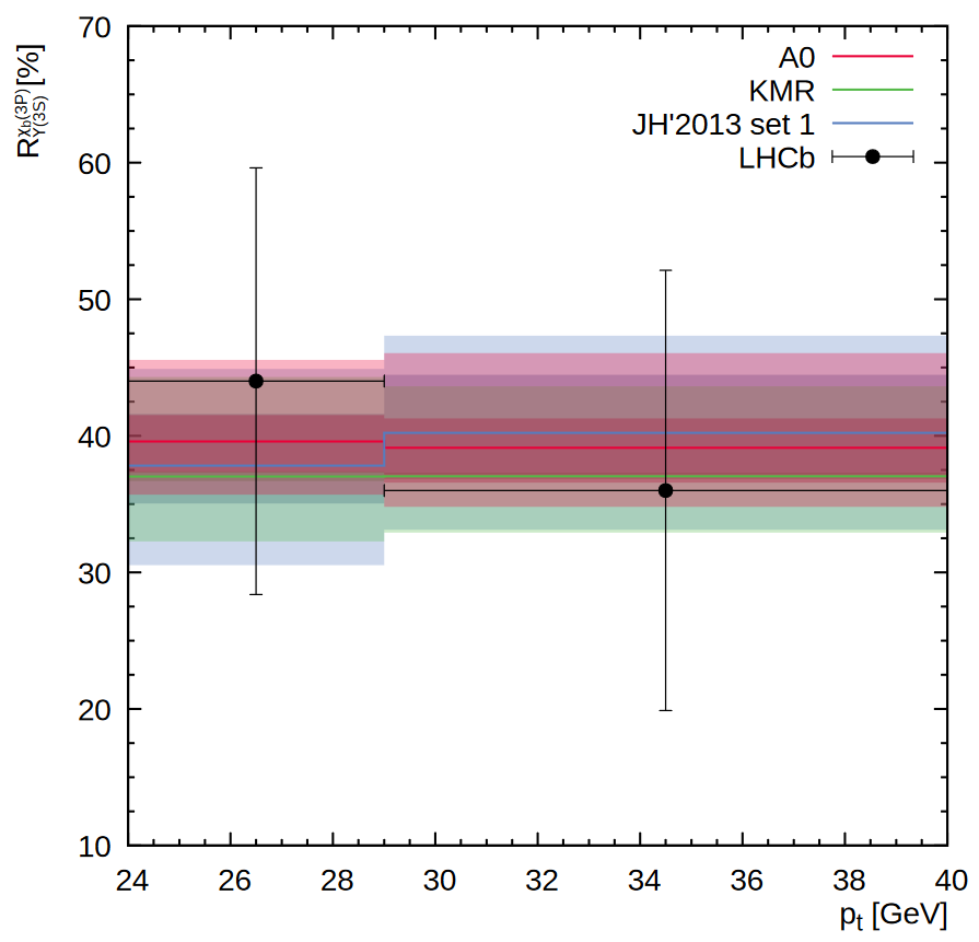
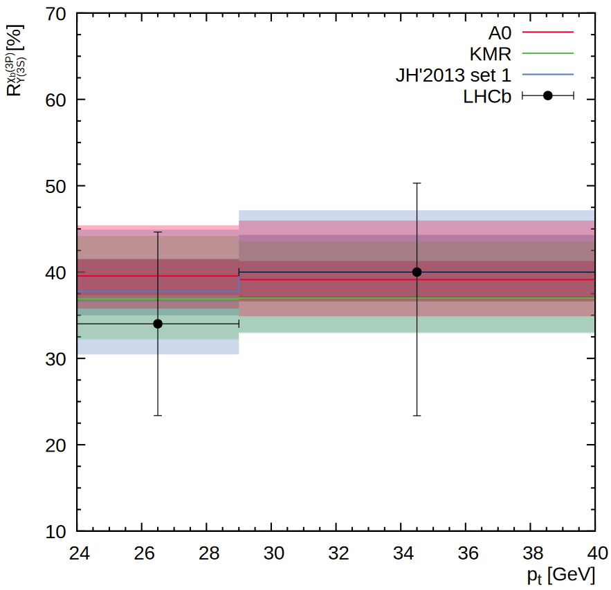
Figure 5: The ratio $R^{\chi_{b}(3P)}_{\Upsilon(3S)}$ calculated as function of $\Upsilon(3S)$ transverse momentum at $\sqrt{s}=7$ TeV (left panel) and $\sqrt{s}=8$ TeV (right panel). Notation of all histograms is the same as in Fig. 3. The experimental data are from LHCb[35].

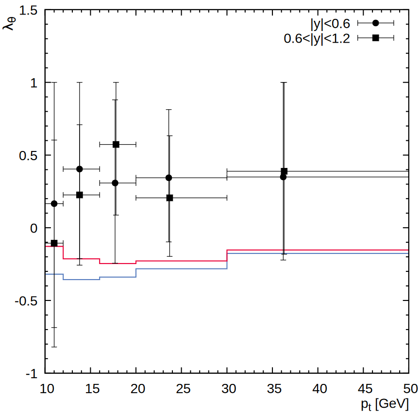
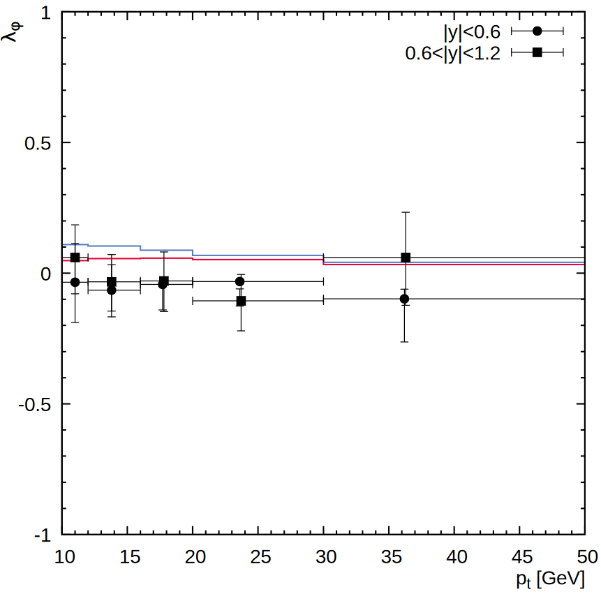
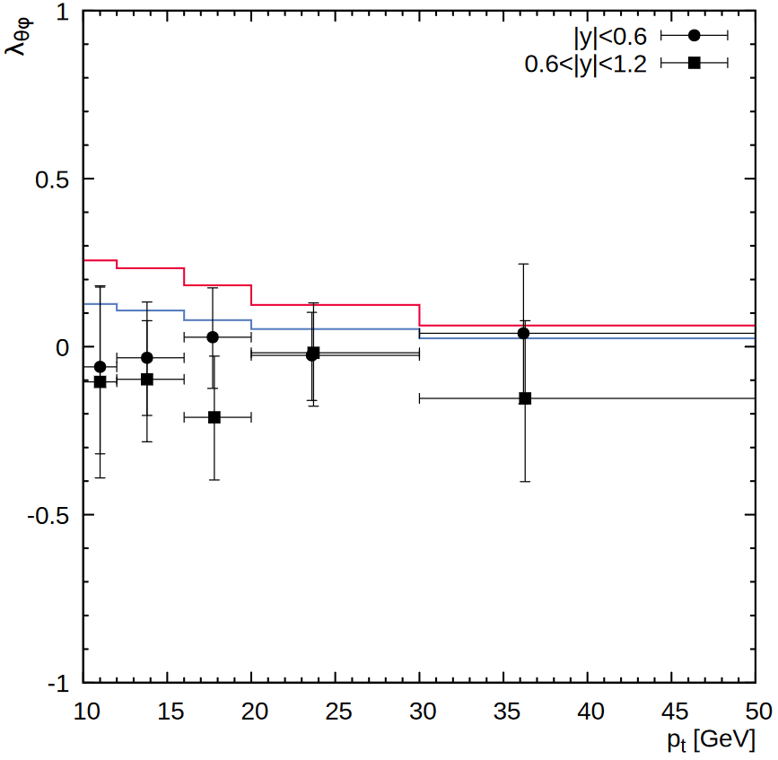
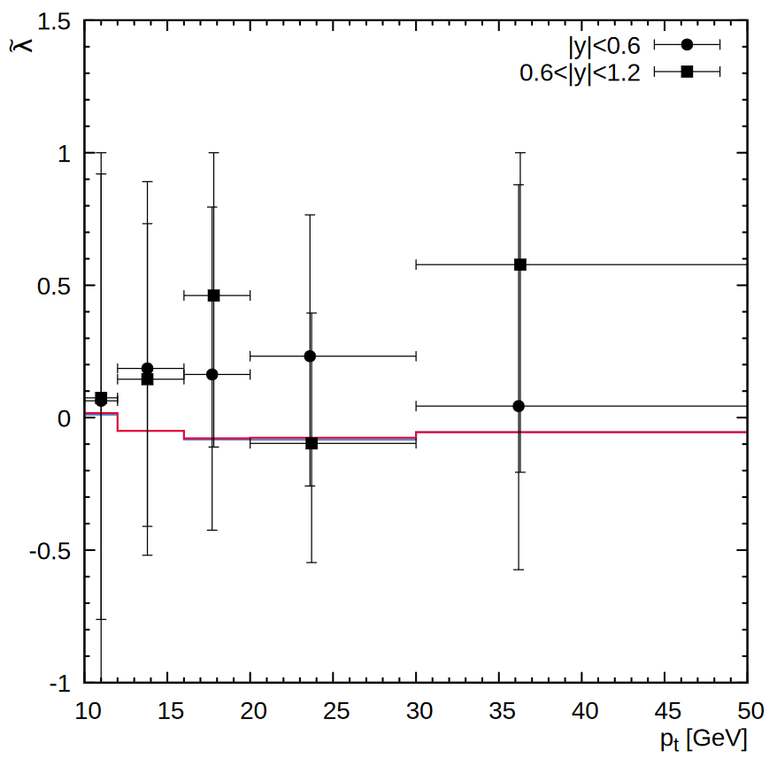
Figure 8: The polarization parameters $\lambda_{\theta}$, $\lambda_{\phi}$, $\lambda_{\theta\phi}$ and $\tilde{\lambda}$ of $\Upsilon(3S)$ mesons calculated in the helicity frame as function of its transverse momentum at $\sqrt{s}=7$ TeV. Notation of all histograms is the same as in Fig. 7. The experimental data are from CMS[28].

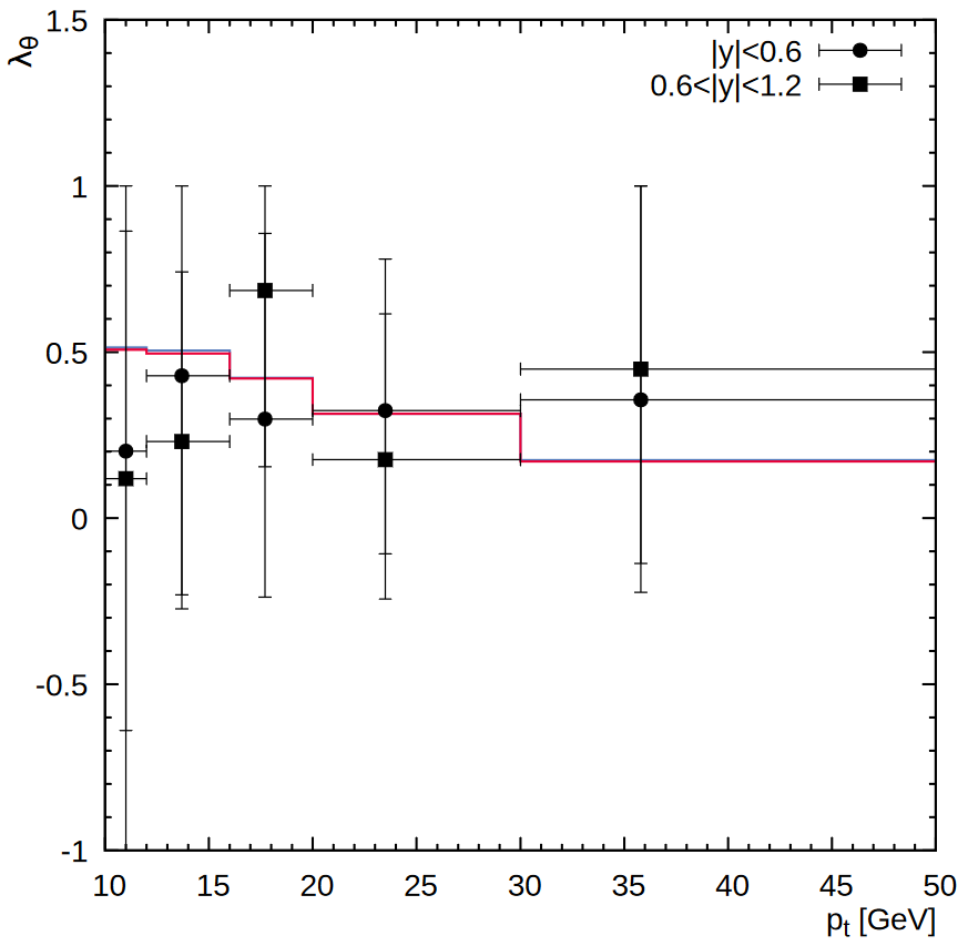
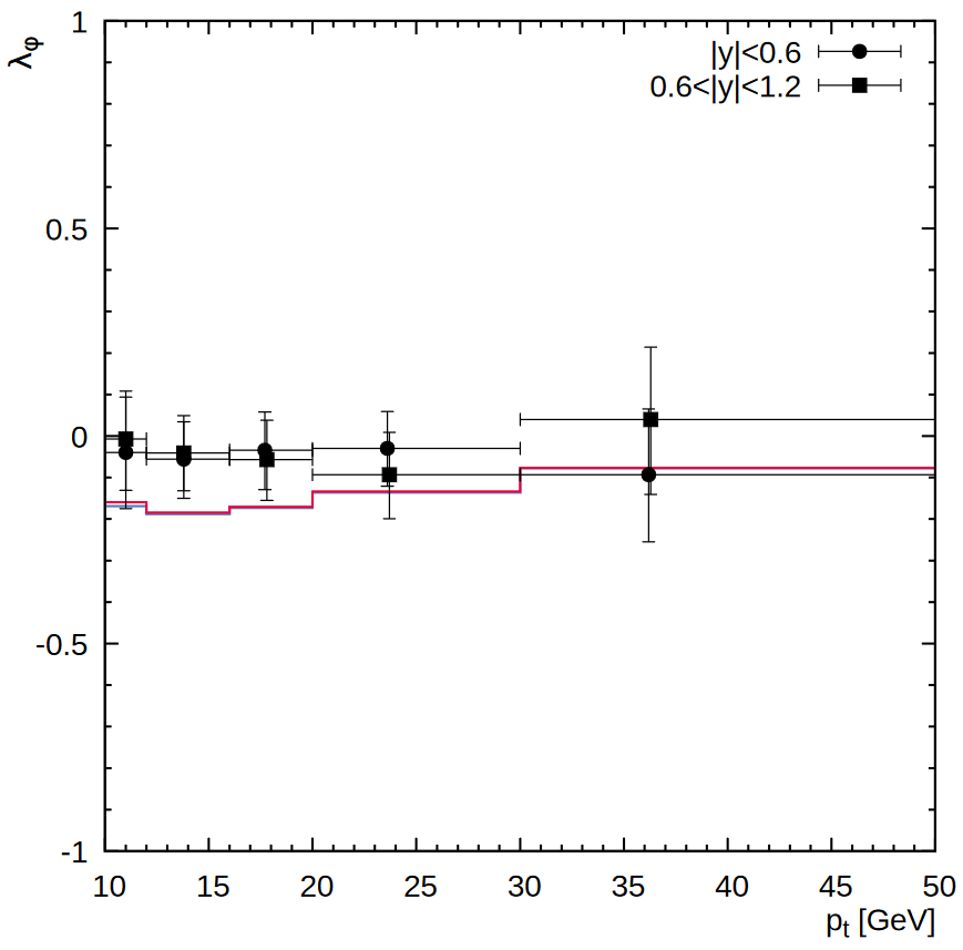
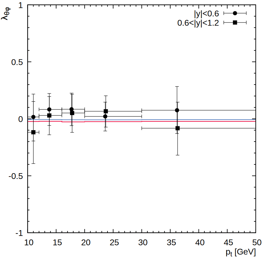
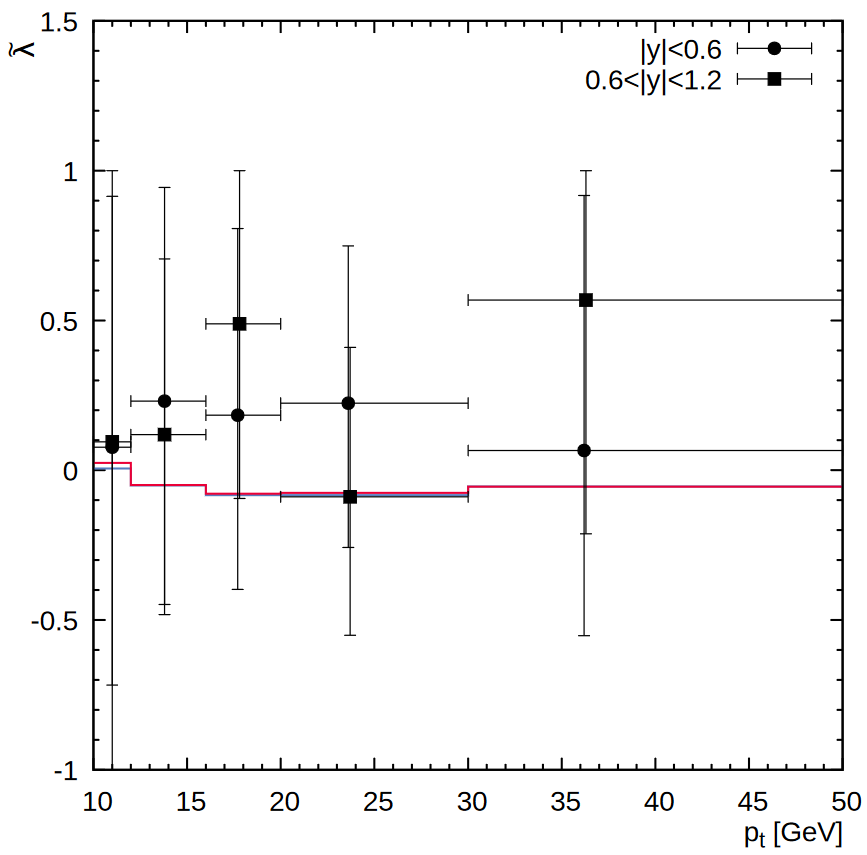
Figure 9: The polarization parameters $\lambda_{\theta}$, $\lambda_{\phi}$, $\lambda_{\theta\phi}$ and $\tilde{\lambda}$ of $\Upsilon(3S)$ mesons calculated in the perpendicular helicity frame as function of its transverse momentum at $\sqrt{s}=7$ TeV. Notation of all histograms is the same as in Fig. 7. The experimental data are from CMS[28].

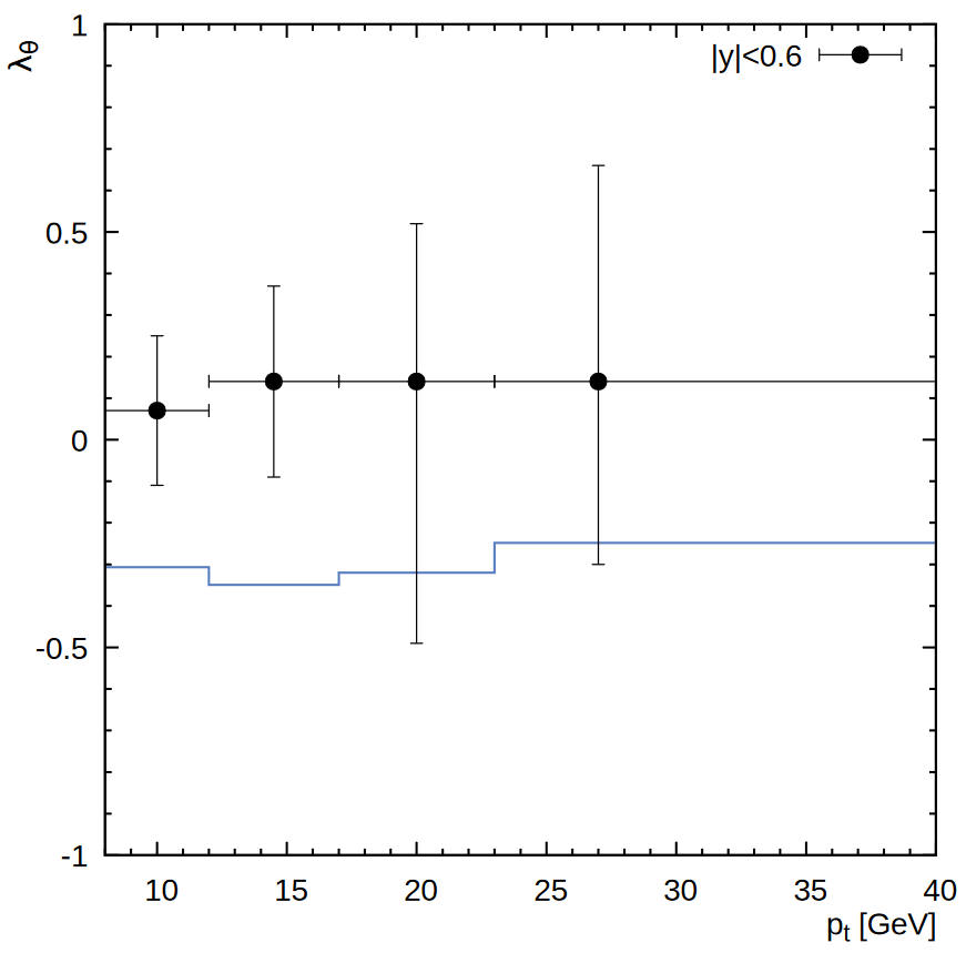
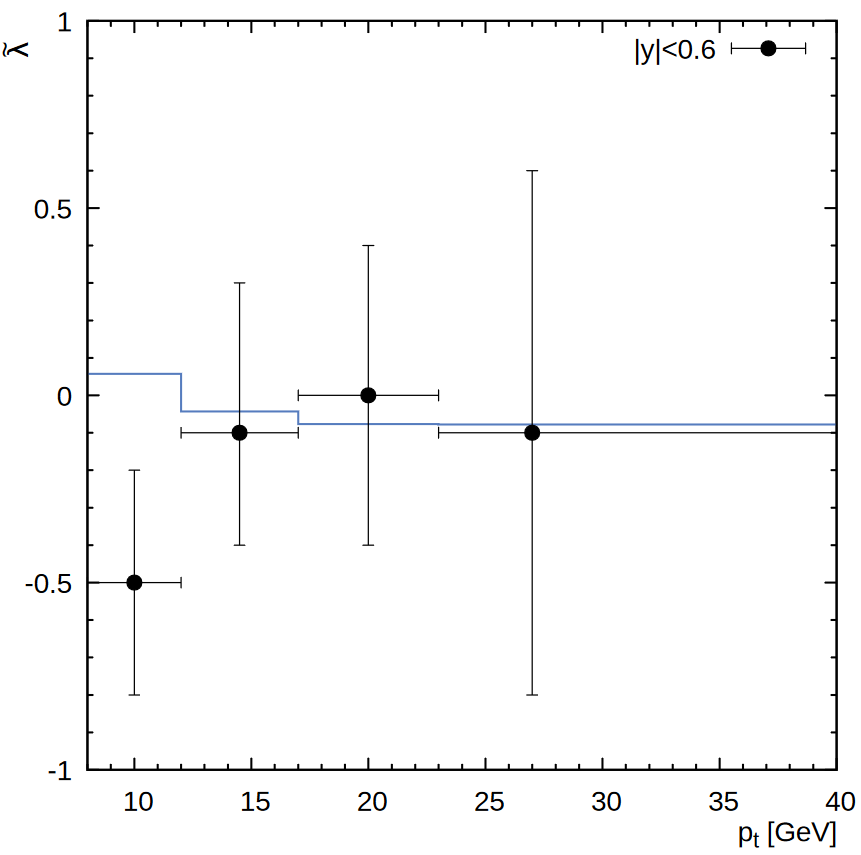
Figure 10: The polarization parameters $\lambda_{\theta}$ and $\tilde{\lambda}$ of $\Upsilon(3S)$ mesons calculated in the helicity frame as function of its transverse momentum at $\sqrt{s}=1.96$ TeV. Notation of all histograms is the same as in Fig. 7. The experimental data are from CDF[42].

References

- [1] G. Bodwin, E. Braaten, G. Lepage, Phys. Rev. D 51, 1125 (1995).
- [2] P. Cho, A.K. Leibovich, Phys. Rev. D 53, 150 (1996); Phys. Rev. D 53, 6203 (1996).
- [3] B. Gong, X.Q. Li, J.-X. Wang, Phys. Lett. B 673, 197 (2009).
- [4] Y.-Q. Ma, K. Wang, K.-T. Chao, Phys. Rev. Lett. 106, 042002 (2011).
- [5] M. Butenschön, B.A. Kniehl, Phys. Rev. Lett. 108, 172002 (2012).
- [6] K.-T. Chao, Y.-Q. Ma, H.-S. Shao, K. Wang, Y.-J. Zhang, Phys. Rev. Lett. 108, 242004 (2012).
- [7] B. Gong, L.-P. Wan, J.-X. Wang, H.-F. Zhang, Phys. Rev. Lett. 110, 042002 (2013).
- [8] Y.-Q. Ma, K. Wang, K.-T. Chao, H.-F. Zhang, Phys. Rev. D 83, 111503 (2011).
- [9] A.K. Likhoded, A.V. Luchinsky, S.V. Poslavsky, Phys. Rev. D 90, 074021 (2014).
- [10] H.-F. Zhang, L. Yu, S.-X. Zhang, L. Jia, Phys. Rev. D 93, 054033 (2016).
- [11] H. Han, Y.-Q. Ma, C. Meng, H.-S. Shao, K.-T. Chao, Phys. Rev. Lett. 114, 092005 (2015).
- [12] H.-F. Zhang, Z. Sun, W.-L. Sang, R. Li, Phys. Rev. Lett. 114, 092006 (2015).
- [13] M. Butenschön, Z. G. He, B.A. Kniehl, Phys. Rev. Lett. 114, 092004 (2015).
- [14] S.S. Biswal, K. Sridhar, J. Phys. G: Nucl. Part. Phys. 39, 015008 (2012).
- [15] A.K. Likhoded, A.V. Luchinsky, S.V. Poslavsky, Mod. Phys. Lett. A 30, 1550032 (2015).
- [16] P. Artoisenet, J. Campbell, J.P. Lansberg, F. Maltoni, F. Tramontano, Phys. Rev. Lett. 101, 152001 (2008).
- [17] J.-P. Lansberg, H.-S. Shao, H.-F. Zhang, Phys. Lett. B 786 342 (2018).
- [18] Y. Feng, J. He, J.-P. Lansberg, H.-S. Shao, A. Usachov, H.-F. Zhang, arXiv:1901.09766 [hep-ph].
- [19] J.-P. Lansberg, arXiv:1903.09185 [hep-ph].
- [20] S.P. Baranov, Phys. Rev. D 93, 054037 (2016).
- [21] S.P. Baranov, A.V. Lipatov, Eur. Phys. J. C 79, 621 (2019).
- [22] S.P. Baranov, A.V. Lipatov, arXiv:1906.07182 [hep-ph].
- [23] CMS Collaboration, Phys. Lett. B 749, 14 (2015).
- [24] CMS Collaboration, Phys. Lett. B 780, 251 (2018).
- [25] ATLAS Collaboration, Phys. Rev. D 87, 052004 (2013).
- [26] LHCb Collaboration, JHEP 1511, 103 (2015).
- [27] LHCb Collaboration, JHEP 1807, 134 (2018).
- [28] CMS Collaboration, Phys. Rev. Lett. 110, 081802 (2013).
- [29] LHCb Collaboration, JHEP 1217, 110 (2017).
- [30] B. Gong, J.-X. Wang, H.-F. Zhang, Phys. Rev. D 83, 114021 (2011).
- [31] K. Wang, Y.-Q. Ma, K.-T. Chao, Phys. Rev. D 85, 114003 (2012).
- [32] B. Gong, L.-P. Wan, J.-X. Wang, H.-F. Zhang, Phys. Rev. Lett. 112, 032001 (2014).
- [33] Y. Feng, B. Gong, L.-P. Wan, J.-X. Wang, H.-F. Zhang, Chin. Phys. C 39, 123102 (2015).
- [34] H. Han, Y.-Q. Ma, C. Meng, H.-S. Shao, Y.-J. Zhang, K.-T. Chao, Phys. Rev. D 94, 014028 (2016).
- [35] LHCb Collaboration, Eur. Phys. J. C 74, 3092 (2014).
-
[36]
S. Catani, M. Ciafaloni, F. Hautmann, Nucl. Phys. B 366, 135 (1991);
J.C. Collins, R.K. Ellis, Nucl. Phys. B 360, 3 (1991). -
[37]
L.V. Gribov, E.M. Levin, M.G. Ryskin, Phys. Rep. 100, 1 (1983);
E.M. Levin, M.G. Ryskin, Yu.M. Shabelsky, A.G. Shuvaev, Sov. J. Nucl. Phys. 53, 657 (1991). -
[38]
E.A. Kuraev, L.N. Lipatov, V.S. Fadin, Sov. Phys. JETP 44, 443 (1976);
E.A. Kuraev, L.N. Lipatov, V.S. Fadin, Sov. Phys. JETP 45, 199 (1977);
I.I. Balitsky, L.N. Lipatov, Sov. J. Nucl. Phys. 28, 822 (1978). -
[39]
M. Ciafaloni, Nucl. Phys. B 296, 49 (1988);
S. Catani, F. Fiorani, G. Marchesini, Phys. Lett. B 234, 339 (1990);
S. Catani, F. Fiorani, G. Marchesini, Nucl. Phys. B 336, 18 (1990);
G. Marchesini, Nucl. Phys. B 445, 49 (1995). - [40] R. Angeles-Martinez et al., Acta Phys. Polon. B 46, 2501 (2015).
- [41] CDF Collaboration, Phys. Rev. Lett. 88, 161802 (2002).
- [42] CDF Collaboration, Phys. Rev. Lett. 108, 151802 (2012).
- [43] S.P. Baranov, A.V. Lipatov, N.P. Zotov, Eur. Phys. J. C 75, 455 (2015).
- [44] S.P. Baranov, A.V. Lipatov, N.P. Zotov, Phys. Rev. D 93, 094012 (2016).
- [45] S.P. Baranov, A.V. Lipatov, Phys. Rev. D 96, 034019 (2017).
-
[46]
C.-H. Chang, Nucl. Phys. B 172, 425 (1980);
E.L. Berger, D.L. Jones, Phys. Rev. D 23, 1521 (1981);
R. Baier, R. Rückl, Phys. Lett. B 102, 364 (1981);
S.S. Gershtein, A.K. Likhoded, S.R. Slabospitsky, Sov. J. Nucl. Phys. 34, 128 (1981). - [47] E.J. Eichten, C. Quigg, arXiv:1904.11542 [hep-ph].
- [48] E.J. Eichten, C. Quigg, Phys. Rev. D 52, 1726 (1995).
- [49] B.A. Kniehl, D.V. Vasin, V.A. Saleev, Phys. Rev. D 73, 074022 (2006).
-
[50]
A.V. Batunin, S.R. Slabospitsky, Phys. Lett B 188, 269 (1987);
P. Cho, M. Wise, S. Trivedi, Phys. Rev. D 51, R2039 (1995). - [51] S.P. Baranov, A.V. Lipatov, M.A. Malyshev, in preparation.
- [52] E. Bycling, K. Kajantie, Particle Kinematics, John Wiley and Sons (1973).
- [53] H. Jung, arXiv:hep-ph/0411287.
- [54] F. Hautmann, H. Jung, Nucl. Phys. B 883, 1 (2014).
-
[55]
M.A. Kimber, A.D. Martin, M.G. Ryskin, Phys. Rev. D 63, 114027 (2001);
A.D. Martin, M.G. Ryskin, G. Watt, Eur. Phys. J. C 31, 73 (2003);
A.D. Martin, M.G. Ryskin, G. Watt, Eur. Phys. J. C 66, 163 (2010). - [56] http://tmd.hepforge.org
- [57] NNPDF Collaboration, Eur. Phys. J. C 77, 663 (2017).
- [58] PDG Collaboration, Phys. Rev. D 98, 030001 (2018).
- [59] S.P. Baranov, A. Szcurek, Phys. Rev. D 77, 054016 (2008).
- [60] B.A. Kniehl, M.A. Nefedov, V.A. Saleev, Phys. Rev. D 94, 054007 (2016).
- [61] www.gnuplot.info
- [62] S.P. Baranov, Phys. Rev. D 91 034011 (2015).
- [63] M. Beneke, M. Krämer, M. Vänttinen, Phys. Rev. D 57, 4258 (1998).