Good-for-MDPs Automata for Probabilistic Analysis and Reinforcement Learning

Abstract

We characterize the class of nondeterministic $\omega$-automata that can be used for the analysis of finite Markov decision processes (MDPs). We call these automata ‘good-for-MDPs’ (GFM). We show that GFM automata are closed under classic simulation as well as under more powerful simulation relations that leverage properties of optimal control strategies for MDPs. This closure enables us to exploit state-space reduction techniques, such as those based on direct and delayed simulation, that guarantee simulation equivalence. We demonstrate the promise of GFM automata by defining a new class of automata with favorable properties—they are Büchi automata with low branching degree obtained through a simple construction—and show that going beyond limit-deterministic automata may significantly benefit reinforcement learning.

1 Introduction

System specifications are often captured in the form of finite automata over infinite words ($\omega$-automata), which are then used for model checking, synthesis, and learning. Of the commonly-used types of $\omega$-automata, Büchi automata have the simplest acceptance condition, but require nondeterminism to recognize all $\omega$-regular languages. Nondeterministic machines can use unbounded look-ahead to resolve nondeterministic choices. However, important applications—like reactive synthesis or model checking and reinforcement learning (RL) for Markov Decision Process (MDPs [25])—have a game setting, which restrict the resolution of nondeterminism to be based on the past.

Being forced to resolve nondeterminism on the fly, an automaton may end up rejecting words it should accept, so that using it can lead to incorrect results. Due to this difficulty, initial solutions to these problems have been based on deterministic automata—usually with Rabin or parity acceptance conditions. For two-player games, Henzinger and Piterman proposed the notion of good-for-games (GFG) automata [15]. These are nondeterministic automata that simulate [23, 14, 9] a deterministic automaton that recognizes the same language. The existence of a simulation strategy means that nondeterministic choices can be resolved without look-ahead.

The situation is better in the case of probabilistic model checking, because the game for which a strategy is sought is played on an MDP against “blind nature,” rather than against a strategic opponent who may take advantage of the automaton’s inability to resolve nondeterminism on the fly. As early as 1985, Vardi noted that probabilistic model checking can be performed with Büchi automata endowed with a limited form of nondeterminism [36]. Limit deterministic Büchi automata (LDBA) [4, 12, 31] perform no nondeterministic choice after seeing an accepting transition. Still, they recognize all $\omega$-regular languages and are, under mild restrictions [31], suitable for probabilistic model checking.

The stronger adversary assumed in two-player games makes good-for-games automata safe for probabilistic model checking, while suitable limit-deterministic Büchi automata (SLDBAs) are not generally safe for two-player games. The question then arises of how to identify the automata that may be used for probabilistic model checking, or, as we shall call them, are good for MDPs (GFM).

We look for other types of nondeterministic Büchi automata (NBA) that are GFM besides the limit-deterministic ones. We start with the observation that the GFM property is preserved by simulation. This gives access to simulation-based statespace reduction. As a side observation, we show that this also holds for good-for-games automata. Simulation-based statespace reduction is a powerful tool for Büchi automata, and, as we do now have Büchi automata to start with—the SLDBAs—we can apply the power of general simulation-based statespace reduction [7, 33, 11, 9]. This includes cheap quotienting (and thus simulation) techniques for the deterministic parts of SLDBAs [27].

In a second step, we consider a simulation game that takes the structure of finite MDPs and properties of games against “blind Nature” into account. This simulation exploits properties of accepting end-components (AECs); we thus refer to it as AEC simulation. This type of simulation does not appear to be suitable for statespace reduction; however, once a GFM automaton $\cal G$ is produced from a language equivalent automaton $\cal A$, it can be used to establish that $\cal A$ is GFM. This may allow us to use the small automaton $\cal A$ instead of the—usually much larger—GFM automaton $\cal G$ that was, e.g., produced by limit determinization.

Finally, we look at a recent application of Büchi automata in RL: In this context, the Büchi acceptance condition of SLDBAs [36] has proven to be more suitable than Rabin or parity conditions [13]. This observation extends to good-for-games Büchi automata, because they are no more expressive than deterministic Büchi automata (DBA) [Sohail08]. The drawback of using SLDBAs is that the transition from the initial to the accepting part often allows for a large number of choices. We use simulation to establish the GFM property of a simple breakpoint-based construction [Miyano84, 26] with a different form of limited nondeterminism: It never offers more than two successors. Experiments suggest that extending the class of GFM automata is beneficial to RL.

Related Work. The production of deterministic and limit deterministic automata for model checking has been intensively studied [26, 24, 1, 28, 35, 34, 29, 31, 8, 32, 20], and several tools are available to produce different types of automata, incl. MoChiBA/Owl [31, 32, 20], LTL3BA [1], GOAL [35, 34], SPOT [8], Rabinizer [19], and Büchifier [17].

So far, only deterministic and a (slightly restricted [31]) class of limit deterministic automata have been considered for probabilistic model checking [36, 4, 12, 31]. Thus, while there have been advances in the efficient production of such automata [12, 31, 32, 20], the consideration of suitable LDBAs by Courcoubetis and Yannakakis in 1988 [3] has been the last time when a fundamental change in the automata foundation of MDP model checking has occurred.

Contribution. The simple but effective observation that simulation preserves the suitability for MDPs (for both traditional simulation and the AEC simulation we introduce) extends the class of automata that can be used in the analysis of MDPs. This provides us with three advantages: The first advantage is that we can now use a wealth of simulation based statespace reduction techniques [7, 33, 11, 9] on an automaton $\cal A$ (e.g. an SLDBA) that we would otherwise use for MDP model checking. The second advantage is that we can use $\cal A$ to check if a different language equivalent automaton, such as an NBA $\cal B$ (e.g. an NBA from which $\cal A$ is derived) simulates $\cal A$. For this second advantage, we can dip into the more powerful class of AEC simulation we define in Section 4 that use properties of winning strategies on finite MDPs. While this is not a complete method for identifying GFM automata, our experimental results indicate that the GFM property is quite frequent for NBAs constructed from random formulas, and can often be established efficiently, while providing a significant statespace reduction and thus offering a significant advantage for model checking.

A third advantage is that we can use the additional flexibility to tailor automata for different applications than model checking, for which specialized automata classes have not yet been developed. We demonstrate this for model-free reinforcement learning (RL). We argue that RL benefits from three propoerties that are less important in model checking: The first—easy to measure—property is a small number of successors, the second and third, are cautiousness, the scope for making wrong decisions, and forgiveness, the resilience against making wrong decisions, respectively.

A small number of successors is a simple and natural goal for RL, as the lack of an explicit model means that the product space of a model and an automaton cannot be evaluated backwards. In a forward analysis, it matters that nondeterministic choices have to be modeled by enriching the decisions in the MDPs with the choices made by the automaton. For LDBAs constructed from NBAs, this means guessing a suitable subset of the reachable states when progressing to the deterministic part of the automaton, meaning a number of choices that is exponential in the NBA. We show that we can instead use slim automata in Section 3.2 as a first example of NBAs that are good-for-MDPs, but not limit deterministic. They have the appealing property that their branching degree is at most two, while keeping the Büchi acceptance mechanism that works well with RL [13]. (Slim automata can also be used for model checking, but they don’t provide similar advantages over suitable LDBAs there, because the backwards analysis used in model checking makes selecting the correct successor trivial.)

Cautiousness and forgiveness are further properties, which are—while harder to quantify—very desirable for RL: LDBAs, for example, suffer from having to make a correct choice when moving into the deterministic part of the automaton, and they have to make this correct choice from a very large set of nondeterministic transitions. While this is unproblematic for standard model checking algorithms that are based on backwards analysis, applications like RL that rely on forward analysis can be badly affected when more (wrong) choices are offered, and when wrong choices cannot be rectified. Cautiousness and forgiveness are a references to this: an automaton is more cautious if it has less scope for making wrong decisions and more forgiving if it allows for correcting previously made decisions (cf. Figure 5 for an example). Our experiments (cf. Section 5) indicate that cautiousness and forgiveness are beneficial for RL.

Organization of the Paper. After the preliminaries, we introduce the “good-for-MDP” property (Section 3) and show that it is preserved by simulation, which enables all minimization techniques that offer the simulation property (Section 3.1). In Section 3.2 we use this observation to construct slim automata—NBAs with a branching degree of 2 that are neither limit deterministic nor good-for-games—as an example of a class of automata that becomes available for MDP model checking and RL. We then introduce a more powerful simulation relation, AEC simulation, that suffices to establish that an automaton is good-for-MDPs (Section 4). In Section 5, we evaluate the impact of the contributions of the paper on model checking and reinforcement learning algorithms.

2 Preliminaries

A nondeterministic Büchi automaton is a tuple ${\cal A}=\langle\Sigma,Q,q_{0},\Delta,\Gamma\rangle$, where $\Sigma$ is a finite alphabet, $Q$ is a finite set of states, $q_{0}\in Q$ is the initial state, $\Delta\subseteq Q\times\Sigma\times Q$ are transitions, and $\Gamma\subseteq Q\times\Sigma\times Q$ is the transition-based acceptance condition.

A run $r$ of ${\cal A}$ on $w\in\Sigma^{\omega}$ is an $\omega$-word $r_{0},w_{0},r_{1},w_{1},\ldots$ in $(Q\times\Sigma)^{\omega}$ such that $r_{0}=q_{0}$ and, for $i>0$, it is $(r_{i-1},w_{i-1},r_{i})\in\Delta$. We write $\operatorname{inf}(r)$ for the set of transitions that appear infinitely often in the run $r$. A run $r$ of ${\cal A}$ is accepting if $\operatorname{inf}(r)\cap\Gamma\neq\emptyset$.

The language, $L_{\mathcal{A}}$, of ${\cal A}$ (or, recognized by ${\cal A}$) is the subset of words in $\Sigma^{\omega}$ that have accepting runs in ${\cal A}$. A language is $\omega$-regular if it is accepted by a Büchi automaton. An automaton ${\cal A}=\langle\Sigma,Q,Q_{0},\Delta,\Gamma\rangle$ is deterministic if $(q,\sigma,q^{\prime}),(q,\sigma,q^{\prime\prime})\in\Delta$ implies $q^{\prime}=q^{\prime\prime}$. ${\cal A}$ is complete if, for all $\sigma\in\Sigma$ and all $q\in Q$, there is a transition $(q,\sigma,q^{\prime})\in\Delta$. A word in $\Sigma^{\omega}$ has exactly one run in a deterministic, complete automaton.

A Markov decision process (MDP) $\mathcal{M}$ is a tuple $(S,A,T,\Sigma,L)$ where $S$ is a finite set of states, $A$ is a finite set of actions, $T:S\times A\to{\cal D}(S)$, where ${\cal D}(S)$ is the set of probability distributions over $S$, is the probabilistic transition function, $\Sigma$ is an alphabet, and $L:S\times A\times S\to\Sigma$ is the labeling function of the set of transitions. For a state $s\in S$, $A(s)$ denotes the set of actions available in $s$. For states $s,s^{\prime}\in S$ and $a\in A(s)$, we have that $T(s,a)(s^{\prime})$ equals $\Pr{}(s^{\prime}|s,a)$.

A run of $\mathcal{M}$ is an $\omega$-word $s_{0},a_{1},\ldots\in S\times(A\times S)^{\omega}$ such that $\Pr{}(s_{i+1}|s_{i},a_{i+1})>0$ for all $i\geq 0$. A finite run is a finite such sequence. For a run $r=s_{0},a_{1},s_{1},\ldots$ we define the corresponding labeled run as $L(r)=L(s_{0},a_{1},s_{1}),L(s_{1},a_{2},s_{2}),\ldots\in\Sigma^{\omega}$. We write $\Omega(\mathcal{M})$ ($\operatorname{Paths}(\mathcal{M})$) for the set of runs (finite runs) of $\mathcal{M}$ and $\Omega_{s}(\mathcal{M})$ ($\operatorname{Paths}_{s}(\mathcal{M})$) for the set of runs (finite runs) of $\mathcal{M}$ starting from state $s$. When the MDP is clear from the context we drop the argument $\mathcal{M}$.

A strategy in $\mathcal{M}$ is a function ${\mu}:\operatorname{Paths}\to{\cal D}(A)$ such that $\operatorname{supp}({\mu}(r))\subseteq A(\operatorname{last}(r))$, where $\operatorname{supp}(d)$ is the support of $d$ and $\operatorname{last}(r)$ is the last state of $r$. Let $\Omega^{\mathcal{M}}_{\mu}(s)$ denote the subset of runs $\Omega^{\mathcal{M}}(s)$ that correspond to strategy ${\mu}$ and initial state $s$. Let $\Sigma_{\mathcal{M}}$ be the set of all strategies. We say that a strategy ${\mu}$ is pure if ${\mu}(r)$ is a point distribution for all runs $r\in\operatorname{Paths}$ and we say that ${\mu}$ is positional if $\operatorname{last}(r)=\operatorname{last}(r^{\prime})$ implies ${\mu}(r)={\mu}(r^{\prime})$ for all runs $r,r^{\prime}\in\operatorname{Paths}$.

The behavior of an MDP $\mathcal{M}$ under a strategy ${\mu}$ with starting state $s$ is defined on a probability space $(\Omega^{\mu}_{s},\mathcal{F}^{\mu}_{s},\Pr^{\mu}_{s})$ over the set of infinite runs of ${\mu}$ from $s$. Given a random variable over the set of infinite runs $f:\Omega\to\mathbb{R}$, we write $\mathbb{E}^{\mu}_{s}\left\{f\right\}$ for the expectation of $f$ over the runs of $\mathcal{M}$ from state $s$ that follow strategy ${\mu}$.

3 Good-for-MDP (GFM) Automata

Given an MDP $\mathcal{M}$ and an automaton $\mathcal{A}=\langle\Sigma,Q,q_{0},\Delta,\Gamma\rangle$, we want to compute an optimal strategy satisfying the objective that the run of $\mathcal{M}$ is in the language of $\mathcal{A}$. We define the semantic satisfaction probability for $\mathcal{A}$ and a strategy ${\mu}$ from state $s$ as:

$$\operatorname{\mathsf{PSem}}^{\mathcal{M}}_{\mathcal{A}}(s,{\mu}) =\Pr{}_{s}^{\mu}\{r{\in}\Omega^{\mu}_{s}:L(r){\in}L_{\mathcal{A}}\}\text{ and} \operatorname{\mathsf{PSem}}^{\mathcal{M}}_{\mathcal{A}}(s) =\sup_{{\mu}}\big{(}\operatorname{\mathsf{PSem}}^{\mathcal{M}}_{\mathcal{A}}(s,{\mu})\big{)}\,.$$

When using automata for the analysis of MDPs, we need a syntactic variant of the acceptance condition. Given an MDP $\mathcal{M}=(S,A,T,\Sigma,L)$ with initial state $s_{0}\in S$ and an automaton $\mathcal{A}=\langle\Sigma,Q,q_{0},\Delta,\Gamma\rangle$, the product $\mathcal{M}\times\mathcal{A}=(S\times Q,(s_{0},q_{0}),A\times Q,T^{\times},\Gamma^{\times})$ is an MDP augmented with an initial state $(s_{0},q_{0})$ and accepting transitions $\Gamma^{\times}$. The function $T^{\times}:(S\times Q)\times(A\times Q)\xrightharpoondown{}{\cal D}(S\times Q)$ is defined by

$$T^{\times}((s,q),(a,q^{\prime}))(({s}^{\prime},{q}^{\prime}))=\begin{cases}T(s,a)({s}^{\prime})&\text{if }(q,L(s,a,{s}^{\prime}),{q}^{\prime})\in\Delta\\ 0&\text{otherwise.}\end{cases}$$

Finally, $\Gamma^{\times}\subseteq(S\times Q)\times(A\times Q)\times(S\times Q)$ is defined by $((s,q),(a,q^{\prime}),(s^{\prime},q^{\prime}))\in\Gamma^{\times}$ if, and only if, $(q,L(s,a,s^{\prime}),q^{\prime})\in\Gamma$ and $T(s,a)(s^{\prime})>0$. A strategy ${\mu}$ on the MDP defines a strategy ${\mu}^{\times}$ on the product, and vice versa. We define the syntactic satisfaction probabilities as

$$\operatorname{\mathsf{PSyn}}^{\mathcal{M}}_{\mathcal{A}}((s,q),{\mu}^{\times}) =\Pr{}_{s}^{\mu}\{r\in\Omega^{{\mu}^{\times}}_{(s,q)}(\mathcal{M}\times\mathcal{A}):\inf(r)\cap\Gamma^{\times}\neq\emptyset\}\enspace,~{}~{}~{}~{}\text{ and}$$

$$\operatorname{\mathsf{PSyn}}^{\mathcal{M}}_{\mathcal{A}}(s) =\sup_{{\mu}^{\times}}\big{(}\operatorname{\mathsf{PSyn}}^{\mathcal{M}}_{\mathcal{A}}((s,q_{0}),{\mu}^{\times})\big{)}\enspace.$$

Note that $\operatorname{\mathsf{PSyn}}^{\mathcal{M}}_{\mathcal{A}}(s)=\operatorname{\mathsf{PSem}}^{\mathcal{M}}_{\mathcal{A}}(s)$ holds for a deterministic $\mathcal{A}$. In general, $\operatorname{\mathsf{PSyn}}^{\mathcal{M}}_{\mathcal{A}}(s)$ $\leq\operatorname{\mathsf{PSem}}^{\mathcal{M}}_{\cal A}(s)$ holds, but equality is not guaranteed because the optimal resolution of nondeterministic choices may require access to future events (see Figure 1).

Definition 1 (GFM automata)

An automaton $\mathcal{A}$ is good for MDPs if, for all MDPs $\mathcal{M}$, $\operatorname{\mathsf{PSyn}}^{\mathcal{M}}_{\mathcal{A}}(s_{0})=\operatorname{\mathsf{PSem}}^{\mathcal{M}}_{\mathcal{A}}(s_{0})$ holds, where $s_{0}$ is the initial state of $\mathcal{M}$.

For an automaton to match $\operatorname{\mathsf{PSem}}^{\mathcal{M}}_{\mathcal{A}}(s_{0})$, its nondeterminism is restricted not to rely heavily on the future; rather, it must possible to resolve the nondeterminism on-the-fly. For example, the Büchi automaton presented on the left of Figure 1, which has to guess whether the next symbol is $\mathtt{a}$ or $\mathtt{b}$, is not good for MDPs, because the simple Markov chain on the right of Figure 1 does not allow resolution of its nondeterminism on-the-fly.

Figure 1: An NBA, which accepts all words over the alphabet $\{a,b\}$, that is not good for MDPs. The dotted transitions are accepting. For the Markov chain on the right where the probability of $a$ and $b$ is $\frac{1}{2}$, the chance that the automaton makes infinitely many correct predictions is $0$

There are three classes of automata that are known to be good for MDPs: (1) deterministic automata, (2) good for games automata [15, 18], and (3) limit deterministic automata that satisfy a few side constraints [4, 12, 31].

A limit-deterministic Büchi automaton (LDBA) is a nondeterministic Büchi automaton (NBA) ${\cal A}=\langle\Sigma,Q_{i}\cup Q_{f},q_{0},\Delta,\Gamma\rangle$ such that $Q_{i}\cap Q_{f}=\emptyset$; $q_{0}\in Q_{i}$; $\Gamma\subseteq Q_{f}\times\Sigma\times Q_{f}$; $(q,\sigma,q^{\prime}),(q,\sigma,q^{\prime\prime})\in\Delta$ and $q,q^{\prime}\in Q_{f}$ implies $q^{\prime}=q^{\prime\prime}$; and $(q,\sigma,q^{\prime})\in\Delta$ and $q\in Q_{f}$ implies $q^{\prime}\in Q_{f}$. An LDBA behaves deterministically once it has seen an accepting transition. Usual LDBA constructions [12, 31] produce GFM automata. We refer to LDBAs with this property as suitable (SLDBAs), cf. Theorem 3.1.

In the context of RL, techniques based on SLDBAs are particularly useful, because these automata use the Büchi acceptance condition, which can be translated to reachability goals. Good for games and deterministic automata require more complex acceptance conditions, like parity, that do not have a natural translation into rewards [13].

Using SLDBA [4, 12, 31] has the drawback that they naturally have a high branching degree in the initial part, as they naturally allow for many different transitions to the accepting part of the LDBA. This can be avoided, but to the cost of a blow-up and a more complex construction and data structure [31]. We therefore propose an automata construction that produces NBAs with a small branching degree—it never produces more than two successors. We call these automata slim. The resulting automata are not (normally) limit deterministic, but we show that they are good for MDPs.

Due to technical dependencies we start with presenting a second observation, namely that automata that simulate language equivalent GFM automata are GFM. As a side result, we observe that the same holds for good-for-games automata. The side result is not surprising, as good-for-games automata were defined through simulation of deterministic automata [15]. But, to the best of our knowledge, the observation from Corollary 1 has not been made yet for good-for-games automata.

3.1 Simulating GFM

An automaton $\cal A$ simulates an automaton $\cal B$ if the duplicator wins the simulation game. The simulation game is played between a duplicator and a spoiler, who each control a pebble, which they move along the edges of $\cal A$ and $\cal B$, respectively. The game is started by the spoiler, who places her pebble on an initial state of $\cal B$. Next, the duplicator puts his pebble on an initial state of $\cal A$. The two players then take turns, always starting with the spoiler choosing an input letter and a transition for that letter in $\cal B$, followed by the duplicator choosing a transition for the same letter in $\cal A$. This way, both players produce an infinite run of their respective automaton. The duplicator has two ways to win a play of the game: if the run of $\cal A$ he constructs is accepting, and if the run the spoiler constructs on $\cal B$ is rejecting. The duplicator wins this game if he has a winning strategy, i.e., a recipe to move his pebble that guarantees that he wins. Such a winning strategy is “good-for-games,” as it can only rely on the past. It can be used to transform winning strategies of $\cal B$, so that, if they were witnessing a good for games property or were good for an MDP, then the resulting strategy for $\mathcal{A}$ has the same property.

Lemma 1 (Simulation Properties)

For $\omega$-automata $\cal A$ and $\cal B$ the following holds.

1. If $\cal A$ simulates $\cal B$ then $\cal L(\cal A)\supseteq\cal L(\cal B)$.

2. If $\cal A$ simulates $\cal B$ and $\cal L(\cal A)\subseteq\cal L(\cal B)$ then $\cal L(\cal A)=\cal L(\cal B)$.

3. If $\cal A$ simulates $\cal B$, $\cal L(\cal A)=\cal L(\cal B)$, and $\cal B$ is GFG, then $\cal A$ is GFG.

4. If $\cal A$ simulates $\cal B$, $\cal L(\cal A)=\cal L(\cal B)$, and $\cal B$ is GFM, then $\cal A$ is GFM.

Proof

Facts (1) and (2) are well known observations. Fact (1) holds because an accepting run of $\mathcal{B}$ on a word $\alpha$ can be translated into an accepting run of $\cal A$ on $\alpha$ by using the winning strategy of $\mathcal{A}$ in the simulation game. Fact (2) follows immediately from Fact (1). Facts (3) and (4) follow by simulating the behaviour of $\mathcal{B}$ on each run. ∎

This observation allows us to use a family of state-space reduction techniques, in particular those based on language preserving translations for Büchi automata based on simulation relation [7, 33, 11, 9]. This requires stronger notions of simulations, like direct and delayed simulation [9]. For the deterministic part of an LDBA, one can also use space reduction techniques for DBAs like [27].

Corollary 1

All statespace reduction techniques that turn an NBA $\cal A$ into an NBA $\cal B$ that simulates $\cal A$ preserve GFG and GFM: if $\cal A$ is GFG or GFM, then $\cal B$ is GFG or GFM, respectively.

3.2 Constructing Slim GFM Automata

Let us fix Büchi automaton $\mathcal{B}=\big{\langle}\Sigma,Q,Q_{0},\Delta,\Gamma\big{\rangle}$. We can write $\Delta$ as a function $\hat{\delta}\colon Q\times\Sigma\to 2^{Q}$ with $\hat{\delta}\colon(q,\sigma)\mapsto\{q^{\prime}\in Q\mid(q,\sigma,q^{\prime})\in\Delta\}$, which can be lifted to sets, using the deterministic transition function $\delta\colon 2^{Q}\times\Sigma\rightarrow 2^{Q}$ with $\delta\colon(S,\sigma)\mapsto\bigcup_{q\in S}\hat{\delta}(q,\sigma)$. We also define an operator, $\mathsf{ndet}$, that translates deterministic transition functions $\delta\colon R\times\Sigma\rightarrow R$ to relations, using

$$\mathsf{ndet}\colon(R\times\Sigma\rightarrow R)\rightarrow 2^{R\times\Sigma\times R}\quad\mbox{ with }\quad\mathsf{ndet}\colon\delta\mapsto\big{\{}(q,\sigma,q^{\prime})\mid q^{\prime}\in\delta(\{q\},\sigma)\big{\}}.$$

This is just an easy means to move back and forth between functions and relations, and helps one to visualize the maximal number of successors. We next define the variations of subset and breakpoint constructions that are used to define the well-known limit deterministic GFM automata—which we use in our proofs—and the slim GFM automata we construct. Let $3^{Q}:=\big{\{}(S,S^{\prime})\mid S^{\prime}\subsetneq S\subseteq Q\big{\}}$ and $3^{Q}_{+}:=\big{\{}(S,S^{\prime})\mid S^{\prime}\subseteq S\subseteq Q\big{\}}$. We define the subset notation for the transitions and accepting transitions as $\delta_{S},\gamma_{S}\colon 2^{Q}\times\Sigma\rightarrow 2^{Q}$ with

$$\delta_{S} \colon(S,\sigma){\mapsto}\big{\{}q^{\prime}\in Q\mid\exists q\in S.\ (q,\sigma,q^{\prime})\in\Delta\big{\}}\text{ and }$$

$$\gamma_{S} \colon(S,\sigma){\mapsto}\big{\{}q^{\prime}\in Q\mid\exists q\in S.\ (q,\sigma,q^{\prime})\in\Gamma\big{\}}.$$

We define the raw breakpoint transitions $\delta_{R}{\colon}3^{Q}{\times}\Sigma{\rightarrow}3^{Q}_{+}$ as $\bigl{(}(S,S^{\prime}),\sigma\bigr{)}{\mapsto}\bigl{(}\delta_{S}(S,\sigma),$ $\delta_{S}(S^{\prime},\sigma)\cup\gamma_{S}(S,\sigma)\bigr{)}$. In this construction, we follow the set of reachable states (first set) and the states that are reachable while passing at least one of the accepting transitions (second set). To turn this into a breakpoint automaton, we reset the second set to the empty set when it equals the first; the transitions where we reset the second set are exactly the accepting ones. The breakpoint automaton $\mathcal{D}=\big{\langle}\Sigma,3^{Q},(Q_{0},\emptyset),\delta_{B},\gamma_{B}\big{\rangle}$ is defined such that, when $\delta_{R}\colon\big{(}(S,S^{\prime}),\sigma\big{)}\mapsto(R,R^{\prime})$, then there are three cases:

1. if $R=\emptyset$, then $\delta_{B}\big{(}(S,S^{\prime})\big{)}$ is undefined (or, if a complete automaton is preferred, maps to a rejecting sink),

2. else, if $R\neq R^{\prime}$, then $\delta_{B}\colon\big{(}(S,S^{\prime}),\sigma\big{)}\mapsto(R,R^{\prime})$ is a non-accepting transition,

3. otherwise $\delta_{B},\gamma_{B}\colon\big{(}(S,S^{\prime}),\sigma\big{)}\mapsto(R^{\prime},\emptyset)$ is an accepting transition.

Finally, we define transitions $\Delta_{SB}\subseteq 2^{Q}\times\Sigma\times 3^{Q}$ that lead from a subset to a breakpoint construction, and $\gamma_{2,1}\colon 3^{Q}\times\Sigma\rightarrow 3^{Q}$ that promote the second set of a breakpoint construction to the first set as follows.

1. $\Delta_{SB}=\Big{\{}\big{(}S,\sigma,(S^{\prime},\emptyset)\big{)}\mid\emptyset\neq S^{\prime}\subseteq\delta_{S}(S,\sigma)\Big{\}}$ are non-accepting transitions,

2. if $\delta_{S}(S^{\prime},\sigma)=\gamma_{S}(S,\sigma)=\emptyset$, then $\gamma_{2,1}\big{(}(S,S^{\prime}),\sigma\big{)}$ is undefined, and

3. otherwise $\gamma_{2,1}\colon\big{(}(S,S^{\prime}),\sigma\big{)}\mapsto\big{(}\delta_{S}(S^{\prime},\sigma)\cup\gamma_{S}(S,\sigma),\emptyset\big{)}$ is an accepting transition.

We can now define standard limit deterministic good for MDP automata.

Theorem 3.1

[12] $\mathcal{A}=\big{\langle}\Sigma,2^{Q}\cup 3^{Q},Q_{0},\mathsf{ndet}(\delta_{S})\cup\Delta_{SB}\cup\mathsf{ndet}(\delta_{B}),\mathsf{ndet}(\gamma_{B})\big{\rangle}$ recognizes the same language as $\mathcal{B}$. It is limit deterministic and good for MDPs.

We now show how to construct a slim GFM Büchi automaton.

Theorem 3.2 (Slim GFM Büchi Automaton)

The automaton

$$\mathcal{S}=\bigl{\langle}\Sigma,3^{Q},(Q_{0},\emptyset),\mathsf{ndet}(\delta_{B})\cup\mathsf{ndet}(\gamma_{2,1}),\mathsf{ndet}(\gamma_{B})\cup\mathsf{ndet}(\gamma_{2,1})\bigr{\rangle}$$

simulates $\cal A$. $\mathcal{S}$ is slim, language equivalent to $\mathcal{B}$, and good for MDPs.

Proof

$\cal S$ is slim: its set of transitions is the union of two sets of deterministic transitions. We show that $\mathcal{S}$ simulates $\mathcal{A}$ by defining a strategy in the simulation game, which ensures that, if the spoiler produces a run $S_{0}\ldots S_{j-1}(S_{j},S_{j}^{\prime})(S_{j+1},S_{j+1}^{\prime})\ldots$ for $\cal A$, then the duplicator produces a run $(T_{0},T_{0}^{\prime})$ $\ldots(T_{j-1},T_{j-1}^{\prime})(T_{j},T_{j}^{\prime})(T_{j+1},T_{j-1}^{\prime})\ldots$ for $\cal S$, such that (1) $S_{i}\subseteq T_{i}$ holds for all $i\in\omega$, and (2) if there are two accepting transitions $\big{(}(S_{k-1},S_{k-1}^{\prime}),\sigma_{k},(S_{k},S_{k}^{\prime})\big{)}$ and $\big{(}(S_{l-1},S_{l-1}^{\prime}),\sigma_{l},(S_{l},S_{l}^{\prime})\big{)}$ with $k<l$, there is an $k<m\leq l$, such that $\big{(}(T_{m-1},T_{m-1}^{\prime}),$ $\sigma_{m}(T_{m},T_{m}^{\prime})\big{)}$ is accepting.

To obtain this, we describe a winning strategy for the duplicator while arguing inductively that it mainains (1). Note that (1) holds initially ($T_{0}=S_{0}$, induction basis).
Initial Phase: Every move of the spoiler—with some letter $\sigma$—that uses a transition from $\delta_{S}$—the subset part of $\cal A$—is followed by a move from $\delta_{B}$ with the same letter $\sigma$. When the duplicator follows this strategy the following holds: when, after a pair of moves, the pebble of the spoiler is on state $S\subseteq Q$, then the pebble of the duplicator is on some state $(S,S^{\prime})$. In particular, (1) is preserved during this phase (induction step).
Transition Phase: The one spoiler move—with some letter $\sigma$—that uses a transition from $\Delta_{SB}$—the transition to the breakpoint part of $\cal A$—is followed by a move from $\delta_{B}$ with the same letter $\sigma$. When the duplicator follows this strategy, and when, after the pair of moves, the pebble of the spoiler is on state $(S,\emptyset)$, then the pebble of the duplicator is on some state $(T,T^{\prime})$ with $S\subseteq T$. In particular, (1) is preserved (induction step).
Final Phase: When the spoiler moves from some state $(S,S^{\prime})$—with some letter $\sigma$—that uses a transition from $\delta_{B}$—the breakpoint part of $\cal A$—to $(\bar{S},\bar{S}^{\prime})$, and when the duplicator is in some state $(T,T^{\prime})$, then the duplicator does the following. He calculates $(\bar{T},\emptyset)=\gamma_{2,1}\big{(}(T,T^{\prime}),\sigma\big{)}$ and checks if $\bar{S}\subseteq\bar{T}$ holds. If $\bar{S}\subseteq\bar{T}$ holds, he plays this transition from $\gamma_{2,1}$ (with the same letter $\sigma$). Otherwise, he plays the transition from $\delta_{B}$ (with the same letter $\sigma$). In either case (1) is preserved (induction step), which closes the inductive argument for (1).

Note that no accepting transition of $\mathcal{A}$ is passed in the initial or tansition phase, so the two accepting transitions from (2) must both fall into the final phase.

To show (2), we first observe that $S_{k}^{\prime}=\emptyset$, and thus $S_{k}^{\prime}\subseteq T_{k}^{\prime}$ holds. Assuming for contradition that all transitions of $\mathcal{S}$ for $\sigma_{k+1}\ldots\sigma_{l-1}$ are non-accepting, we obtain—using (1)—by a straightforward inductive argument that $S_{i}^{\prime}\subseteq T_{i}^{\prime}$ for all $i$ with $k{\leq}i{<}l$. (Note that transitions in $\delta_{B}$ are accepting when they are also be in $\gamma_{B}$.)

Using that $S_{l}=\delta_{S}(S_{l-1}^{\prime},\sigma_{l})\cup\gamma_{S}(S_{l-1},\sigma_{l})\subseteq\delta_{S}(T_{l-1}^{\prime},\sigma_{l})\cup\gamma_{S}(T_{l-1},\sigma_{l})$ holds, the spoiler uses an accepting transition from $\gamma_{2,1}$ in this step.

Using Lemma 1, it now suffices to show that the language of $\mathcal{S}$ is included in the language of $\mathcal{B}$. To show this, we simply argue that an accepting run $\rho=(Q_{0},Q_{0}^{\prime}),(Q_{1},Q_{1}^{\prime}),$ $(Q_{2},Q_{2}^{\prime}),(Q_{3},Q_{3}^{\prime}),\ldots$ of $\mathcal{S}$ on an input word $\alpha=\sigma_{0},\sigma_{1},\sigma_{2},\ldots$ can be interpreted as a forest of finitely many finitely branching trees of overall infinite size, where all infinite branches are accepting runs of $\mathcal{B}$. Kőnig’s Lemma then proves the existence of an accepting run of $\mathcal{B}$.

This forest is the usual one. The nodes are labeled by states of $\mathcal{B}$, and the roots (level 0) are the initial states of $\mathcal{B}$. Let $I=\bigl{\{}i\in\mathbb{N}\mid\big{(}(Q_{i-1},Q_{i-1}^{\prime}),\sigma_{i-1},(Q_{i},Q_{i}^{\prime})\big{)}\in\Gamma:=\mathsf{ndet}(\gamma_{B})\cup\mathsf{ndet}(\gamma_{2,1})\bigr{\}}$ be the set of positions after accepting transitions in $\rho$. We define the predecessor function $\mathsf{pred}\colon\mathbb{N}\rightarrow I\cup\{0\}$ with $\mathsf{pred}\colon i\mapsto\max\big{\{}j\in I\cup\{0\}\mid j<i\big{\}}$.

We call a node with label $q_{l}$ on level $l$ an end-point if one of the following applies: (1) $q_{l}\notin Q_{l}$ or (2) $l\in I$ and for all $j$ such that $\mathsf{pred}(l)\leq j<l$, where $q_{j}$ is the label of the ancestor of this node on level $j$, we have $(q_{j},\sigma_{j},q_{j+1})\notin\Gamma$.

(1) may only happen after a transition from $\gamma_{2,1}$ has been taken, and the $q_{l}$ is not among the states that is traced henceforth. (2) identifies parts of the run tree that do not contain an accepting transition.

A node labeled with $q_{l}$ on level $l$ that is not an endpoint has $\big{|}\delta_{S}(q_{l},\sigma_{l})\big{|}$ children, labeled with the different elements of $\delta_{S}(q_{l},\sigma_{l})$. It is now easy to show by induction over $i$ that the following holds.

1. For all $q\in Q_{i}$, there is a node on level $i$ labeled with $q$.

2. For $i\notin I$ and $q\in Q_{i}^{\prime}$, there is a node labeled $q$ on level $i$, a $j$ with $\mathsf{pred}(i)\leq j<i$, and ancestors on level $j$ and $j+1$ labeled $q_{j}$ and $q_{j+1}$, such that $(q_{j},\sigma_{j},q_{j+1})\in\Gamma$. (The ‘ancestor’ on level $j+1$ might be the state itself.)

   For $i\in I$ and $q\in Q_{i}^{\prime}$, there is a node labeled $q$ on level $i$, which is not an end point.

Consequently, the forest is infinite, finitely branching, and finitely rooted, and thus contains an infinite path. By construction, this path is an accepting run of $\cal B$. ∎

Figure 2: An NBA for $\operatorname{\mathsf{G}}\operatorname{\mathsf{F}}a$ (in the upper right corner) together with an SLDBA and a slim NBA constructed from it. The SLDBA and the slim NBA are shown sharing their common part. State $\{0,1\}$, produced by the subset construction, is the initial state of the SLDBA, while state $(\{0,1\},\emptyset)$—the initial state of the breakpoint construction—is the initial state of the slim NBA. States $(\{1\},\emptyset)$ and $(\{0\},\emptyset)$ are states of the breakpoint construction that only belong to the SLDBA because they are not reachable from $(\{0,1\},\emptyset)$. The transitions out of $\{0,1\}$, except the self loop, belong to $\Delta_{SB}$. The dashed-line transition from $(\{0,1\},\{0\})$ belongs to $\gamma_{2,1}$

The resulting automata are simple in structure and enable symbolic implementation (See Fig. 2). It cannot be expected that there are much smaller good for MDP automata, as its explicit construction is the only non-polynomial part in model checking MDPs.

Theorem 3.3

Constructing a GFM Büchi automaton $G$ that recognizes the models of an LTL formula $\varphi$ requires time doubly exponential in $\varphi$, and constructing a GFM Büchi automaton $G$ that recognizes the language of an NBA $\mathcal{B}$ requires time exponential in $\mathcal{B}$.

Proof

As resulting automata are GFM, they can be used to model check MDPs $\cal M$ against this property, with cost polynomial in product of $\cal M$ and $\cal G$. If $\cal G$ could be produced faster (and if they could, consequently be smaller) than claimed, it will contradict the 2-ExpTime- and ExpTime-hardness [4] of these model checking problems. ∎

It appears reasonable to assume that these GFM automata are exponential and doubly exponential in the size of the automaton and formula, respectively. However, in principle they could be smaller, as long as establishing the non-trivial GFM property is sufficiently expensive.

4 Accepting End-Component Simulation

An end-component [5, 2] of an MDP $\mathcal{M}$ is a sub-MDP $\mathcal{M}^{\prime}$ of $\mathcal{M}$ such that its underlying graph is strongly connected. A maximal end-component is maximal under set-inclusion. Every state of an MDP belongs to at most one maximal end-component.

Theorem 4.1 (End-Component Properties. Theorem 3.1 and Theorem 4.2 of [5])

Once an end-component $C$ of an MDP is entered, there is a strategy that visits every state-action combination in $C$ infinitely often with probability $1$ and stays in $C$ forever.

For a product MDP, an accepting end-component (AEC) is an end-component that contains some transition in $\Gamma^{\times}$. There is a positional pure strategy for an AEC $C$ that surely stays in $C$ and almost surely visits a transition in $\Gamma^{\times}$ infinitely often.

For a product MDP, there is a set of disjoint accepting end-components such that, from every state, the maximal probability to reach the union of these accepting end-components is the same as the maximal probability to satisfy $\Gamma^{\times}$. Moreover, this probability can be realized by combining a positional pure (reachability) strategy outside of this union with the aforementioned positional pure strategies for the individual AECs.

Lemma 1 shows that the GFM property is preserved by simulation: For language-equivalent automata $\mathcal{A}$ and $\mathcal{B}$, if $\mathcal{A}$ simulates $\mathcal{B}$ and $\mathcal{B}$ is GFM, then $\mathcal{A}$ is also GFM. However, a GFM automaton may not simulate a language-equivalent GFM automaton. (See Figure 3.) Therefore we introduce a coarser preorder, Accepting End-Component (AEC) simulation, that exploits the finiteness of the MDP $\mathcal{M}$. We rely on Theorem 4.1 to focus on positional pure strategies for $\mathcal{M}\times\mathcal{B}$. Under such strategies, $\mathcal{M}\times\mathcal{B}$ becomes a Markov chain [2] such that almost all its runs have the following properties:

• They will eventually reach a leaf strongly connected component (LSCC) in the Markov chain.

• If they have reached a LSCC $L$, then, for all $\ell\in\mathbb{N}$, all sequences of transitions of length $\ell$ in $L$ occur infinitely often, and no other sequence of length $\ell$ occurs.

With this in mind, we can intuitively ask the spoiler to pick a run through this Markov chain, and to disclose information about this run. Specifically, we can ask her to signal when she has reached an accepting LSCC in the Markov chain, and to provide information about this LSCC, in particular information entailed by the full list of sequences of transitions of some fixed length $\ell$ described above. Runs that can be identified to either not reach an accepting LSCC, to visit transitions not in this list, or to visit only a subset of sequences from this list, form a $0$ set. In the simulation game we define below, we make use of this observation to discard such runs.

A simulation game can only use the syntactic material of the automata—-neither the MDP nor the strategy are available. The information the spoiler may provide cannot explicitly refer to them. What the spoiler may be asked to provide is information on when she has entered an accepting LSCC, and, once she has signaled this, which sequences of length $l$ of automata transitions of $\mathcal{B}$ occur in the LSCC. The sequences of automata transitions are simply the projections on the automata transitions from the sequences of transitions of length $\ell$ that occur in the LSCC $L$. We call this information a gold-brim accepting end-component claim of length $\ell$, $\ell$-GAEC claim for short.

The term “gold-brim” in the definition indicates that this is a powerful approach, but not one that can be implemented efficiently. We will define weaker, efficiently implementable notions of accepting end-component claims (AEC claims) later.

The AEC simulation game is very similar to the simulation game of Section 3.1. Both players produce an infinite run of their respective automata. If the spoiler makes an AEC claim, e.g., an $\ell$-GAEC claim, we say that her run complies with it if, starting with the transition when the AEC claim is made, all states, transitions, or sequences of transitions in the claim appear infinitely often, and all states, transitions, and sequences of transitions the claim excludes do not appear. For an $\ell$-GAEC claim, this means that all of the sequences of transitions of length $\ell$ in the claim occur infinitely often, and no other sequence of length $\ell$ occurs henceforth.

Thus, like a classic simulation game, an $\ell$-GAEC simulation game is started by the spoiler, who places her pebble on an initial state of $\cal B$. Next, the duplicator puts his pebble on an initial state of $\cal A$. The two players then take turns, always starting with the spoiler choosing an input letter and an according transition from $\cal B$, followed by the duplicator choosing a transition for the same letter in $\cal A$.

Different from the classic simulation game, in an $\ell$-GAEC simulation game, the spoiler has an additional move that she can (and, in order to win, has to) perform once in the game: In addition to choosing a letter and a transition, she can claim that she has reached an accepting end-component, and provide a complete list of sequences of automata transitions of length $\ell$ that can henceforth occur. This store is maintained, and never updated. It has no further effect on the rules of the game: Both players produce an infinite run of their respective automata. The duplicator has four ways to win:

1. if the spoiler never makes an AEC claim,

2. if the run of $\mathcal{A}$ he constructs is accepting,

3. if the run the spoiler constructs on $\mathcal{B}$ does not comply with the AEC claim, and

4. if the run that the spoiler produces is not accepting.

For $\ell$-GAEC claims, (4) simply means that the set of transitions defined by the sequences does not satisfy the Büchi, parity, or Rabin acceptance condition.

Theorem 4.2

[$\ell$-GAEC Simulation] If $\cal A$ and $\cal B$ are language equivalent automata, $\cal B$ is GFM, and there exists an $\ell$ such that $\cal A$ $\ell$-GAEC simulates $\cal B$, then $\cal A$ is GFM.

For the proof, we use an arbitrary (but fixed) MDP $\cal M$, and an arbitrary (but fixed) pure optimal positional strategy ${\mu}$ for $\cal M\times\cal B$, resulting in the Markov chain $(\cal M\times\cal B)_{\mu}$. We assume w.l.o.g. that the accepting LSCCs in $(\cal M\times\cal B)_{\mu}$ are identified, e.g., by a bit.

Let $\tau$ be a winning strategy of the duplicator in an $\ell$-GAEC simulation game. Abusing notation, we let $\tau\circ{\mu}$ denote the finite-memory strategy obtained from ${\mu}$ and $\tau$ for $\cal M\times\cal A$, where $\tau$ is acting only on the automata part of $(\cal M\times\cal B)$, and where the spoiler makes the move to the end-component when she is in some LSCC $B$ of $(\cal M\times\cal B)_{\mu}$ and gives the full list of sequences of transitions of length $\ell$ that occur in $B$.

Proof

As $\cal B$ is good for MDPs, we only have to show that the chance of winning in $(\cal M\times\cal A)_{\tau\circ{\mu}}$ is at least the chance of winning in $(\cal M\times\cal B)_{\mu}$. The chance of winning in $(\cal M\times\cal B)_{\mu}$ is the chance of reaching an accepting LSCC in $(\cal M\times\cal B)_{\mu}$. It is also the chance of reaching an accepting LSCC $L\in(\cal M\times\cal B)_{\mu}$ and, after reaching $L$, to see exactly the sequences of transitions of length $\ell$ that occur in $L$, and to see all of them infinitely often.

By construction, $\tau\circ{\mu}$ will translate those runs into accepting runs of $(\cal M\times\cal A)_{\tau\circ{\mu}}$, such that the chance of an accepting run of $(\cal M\times\cal A)_{\tau\circ{\mu}}$ is at least the chance of an accepting run of $(\cal M\times\cal B)_{\mu}$. As ${\mu}$ is optimal, the chance of winning in $\cal M\times\cal A$ is at least the chance of winning in $\cal M\times\cal B$. As $\cal B$ is GFM, this is the chance of $\cal M$ producing a run accepted by $\cal B$ (and thus $\cal A)$ when controlled optimally, which is an upper bound on the chance of winning in $\cal M\times\cal A$. ∎

An $\ell$-GAEC simulation, especially for large $\ell$, results in very large state spaces, because the spoiler has to list all sequences of transitions of $\mathcal{B}$ of length $\ell$ that will appear infinitely often. No other sequence of length $\ell$ may then appear in the run. This can, of course, be prohibitively expensive.

As a compromise, one can use coarser-grained information at the cost of reducing the duplicator’s ability of winning the game. E.g., the spoiler could be asked to only reveal a transition that is repeated infinitely often, plus (when using more powerful acceptance conditions than Büchi), some acceptance information, say the dominating priority in a parity game or a winning Rabin pair. This type of coarse-grained claim can be refined slightly by allowing the duplicator to change at any time the transition that is to appear infinitely often to the transition just used by the spoiler. Generally, we say that an AEC simulation game is any simulation game, where

• the spoiler provides a list of states, transitions, or sequences of transitions that will occur infinitely often and a list of states, transitions, or sequences of transitions that will not occur in the future when making her AEC claim, and

• the duplicator may be able to update this list based on his observations,

• there exists some $\ell$-GAEC simulation game such that a winning strategy of the spoiler translates into a winning strategy of the spoiler in the AEC simulation game.

The requirement that a winning spoiler strategy translates into a winning spoiler strategy in an $\ell$-GAEC game entails that AEC simulation games can prove the GFM property.

Corollary 2

[AEC Simulation] If $\cal A$ and $\cal B$ are language equivalent automata, $\cal B$ is good for MDPs, and $\cal A$ AEC-simulates $\cal B$, then $\cal A$ is good for MDPs.

Of course, for every AEC simulation, one first has to prove that winning strategies for the spoiler translate. We have used two simple variations of the AEC simulation games:

accepting transition: the spoiler may only make her AEC claim when taking an accepting transition; this transition—and no other information—is stored, and the spoiler commits to—and commits only to—seeing this transition infinitely often;
accepting transition with update: different to the accepting transition AEC simulation game, the duplicator can—but does not have to—update the stored accepting transition whenever the spoiler passes by an accepting transition.

Theorem 4.3

Both, the accepted transition and the accepted transition with update AEC simulation, can be used to establish the good for MDPs property.

To show this, we describe the strategy translations in accordance with Corollary 2.

Proof

In both cases, the translation of a winning strategy of the spoiler for the $1$-GAEC simulation game are straightforward: The spoiler essentially follows her winning strategy from the $1$-GAEC simulation game, with the extra rule that she will make her AEC claim to the duplicator on the first accepting transition on or after her AEC claim in the $1$-GAEC claim. If the duplicator is allowed to update the transition, this information is ignored by the spoiler—she plays according to her winning strategy from the $1$-GAEC simulation game. Naturally, the resulting play will comply with her $1$-GAEC claim, and will thus also be winning for the—weaker—AEC claim made to the duplicator. ∎

Figure 3: Automata $\cal A$ (left) and $\cal B$ (right) for $\varphi=(\operatorname{\mathsf{G}}\operatorname{\mathsf{F}}\mathtt{a})\vee(\operatorname{\mathsf{G}}\operatorname{\mathsf{F}}\mathtt{b})$. The dotted transitions are accepting. The NBA $\cal A$ does not simulate the DBA $\cal B$: $\mathcal{B}$ can play $a$’s until $\mathcal{A}$ moves to either the state on the left, or the state on the right. $\mathcal{B}$ then wins by henceforth playing only $b$’s or only $a$’s. However, $\mathcal{A}$ is good for MDPs. It wins the AEC simulation game by waiting until an AEC is reached (by $\cal B$), and then check if $a$ or $b$ occurs infinitely often in this AEC. Based on this knowledge, $\cal A$ can make its decision. This can be shown by AEC simulation if $\cal B$ has to provide sufficient information, such as a list of transitions—or even a list of letters—that occur infinitely often. The amount of information the spoiler has to provide determines the strength of the AEC simulation used. If, e.g., $\cal B$ only has to reveal one accepting transition of the end-component, then it can select an end-component where the revealed transition is $(b_{1},c,b_{0})$, which does not provide sufficient information. Whereas, if the duplicator is allowed to update the transition, then the duplicator wins by updating the recorded transition to the next $a$ or $b$ transition

We use AEC simulation to identify GFM automata among the automata produced (e.g., by SPOT [8]) at the beginning of the transformation. Figure 3 shows an example for which the duplicator wins the AEC simulation game, but loses the ordinary simulation game. Candidates for automata to simulate are, e.g., the slim GFM Büchi automata and the limit deterministic Büchi automata discussed above.

5 Evaluation

5.1 General Büchi Automata for Probabilistic Model Checking

As discussed, automata that simulate slim automata or SLDBAs are good for MDPs. This fact can be used to allow Büchi automata produced from general-purpose tools such as SPOT’s [8] ltl2tgba rather than using specialized automata types. Automata produced by such tools are often smaller because such general-purpose tools are highly optimized and not restricted to producing slim or limit deterministic automata. Thus, one produces an arbitrary Büchi automaton using any available method, then transforms this automaton into a slim or limit deterministic automaton, and finally checks whether the original automaton simulates the generated one.

We have evaluated this idea on random LTL formulas produced by SPOT’s tool randltl. We have set the tree size, which influences the size of the formulas, to 50, and have produced 1000 formulas with 4 atomic propositions each. We left the other values to their defaults. We have then used SPOT’s ltl2tgba (version 2.7) to turn these formulas into non-generalized Büchi automata using default options. Finally, for each automaton, we have used our tool to check whether the automaton simulates a limit deterministic automaton that we produce from this automaton. For comparison, we have also used Owl’s [31] tool ltl2ldba (version 19.06.03) to compute limit deterministic non-generalized Buchi automata. We have also used the option of this tool to compute Büchi automata with a nondeterministic initial part. We used 10 minute timeouts.

Of these 1000 formulas, 315 can be transformed to deterministic Büchi automata. For an additional 103 other automata generated, standard simulation sufficed to show that they are GFM. For a further 11 of them, the simplest AEC simulation (the spoiler chooses an accepting transition to occur infinitely often) sufficed, and another 1 could be classed GFM by allowing the duplicator to update the transition. 501 automata turned out to be nonsimulatable and for 69 we did not get a decision due to a timeout.

For the LTL formulas for which ltl2tgba could not produce deterministic automata, but for which simulation could be shown, the number of states in the generated automata was often lower than the number of states in the automata produced by Owl’s tools. On average, the number of states per automaton was $\approx$15.21 for SPOT’s ltl2tgba; while for Owl’s ltl2ldba it was $\approx$46.35. We provide examples for each outcome in Table 1.

Figure 4: Deciles ratio ltl2tgba
/semi-deterministic automata

Let us consider the ratio between the size of automata produced by ltl2tgba and the size of semi-deterministic automata produced by Owl. The average of this number for all automata that are not deterministic and that can be simulated in some way is $\approx{}1.0335$. This means that on average, for these automata, the semi-deterministic automata are slightly smaller. If we take a look at the first $5$ deciles depicted in Fig. 4, we see that there is a large number of formulas for which ltl2tgba and Owl produce automata of the same size. For around $24.3478\%$ of the cases, automata by SPOT are smaller than those produced by Owl (ratio $<1$).

Table 1: Simulation results. Column “LTL” contains the formula the automata are generated from. Column “sim” contains the type of simulation required to show that the original automaton is suitable for MDPs. There, “det” means that the automaton is deterministic (no simulation required), “sim0” means that standard simulation sufficed, “sim1” means that the simulation where the spoiler is forced to choose a transition to be repeated infinitely often suffices, “sim2” means that in addition the witness can change the transition which has to occur infinitely often, and “nosim” means that we were not able to prove a simulation relation. “ltl2tgba” contains the number of states from SPOT’s ltl2tgba, “owl” the ones from Owl’s ltl2ldba

ltl	sim	ltl2tgba	owl
$\displaystyle\autobreak(\mathsf{X}\mathsf{F}(\mathit{ap}_{3}\mathsf{\rightarrow}(\lnot\mathit{ap}_{0}\lor\lnot\mathsf{G}\lnot\mathit{ap}_{2}))\land\lnot((\mathit{ap}_{1}\mathsf{\rightarrow}\mathit{ap}_{3})\mathsf{R}\mathsf{G}\mathit{ap}_{1}))\lor((\mathsf{F}\mathit{ap}_{2}\mathsf{W}\mathit{ap}_{1})\land(\mathsf{G}\mathit{ap}_{3}\mathsf{M}\mathit{ap}_{3}))$	det	7	10
$\displaystyle\autobreak\mathsf{G}\mathsf{F}\mathsf{G}(\lnot\mathit{ap}_{3}\lor\mathsf{X}\mathsf{X}\mathsf{X}(\mathit{ap}_{0}\mathbin{\mathsf{U}}(\mathit{ff}\mathsf{R}\mathit{ap}_{2})))\mathsf{R}\mathsf{F}\mathsf{G}\mathit{ap}_{1}$	sim0	2	2
$\displaystyle\autobreak\lnot\mathsf{G}\mathsf{F}\lnot(\mathsf{X}(\mathit{ap}_{1}\mathsf{\leftrightarrow}(\mathit{tt}\mathbin{\mathsf{U}}\mathsf{X}\mathit{ap}_{2}))\mathsf{xor}\mathsf{X}(\mathit{ff}\mathsf{R}(\lnot\mathit{ap}_{0}\mathsf{\leftrightarrow}\mathsf{G}\mathsf{X}\mathit{ap}_{3})))$	sim1	26	14
$\displaystyle\autobreak\mathsf{F}\mathsf{G}(\lnot(\mathsf{F}\mathit{ap}_{2}\mathsf{R}(\mathit{ap}_{1}\land\mathsf{G}\mathit{ap}_{0}))\mathsf{\rightarrow}(\mathit{ap}_{3}\mathsf{xor}\mathsf{G}\mathit{ap}_{1}))\mathsf{\leftrightarrow}(\mathsf{G}\mathit{ap}_{2}\land(\mathsf{F}\mathsf{X}\mathit{ap}_{0}\mathbin{\mathsf{U}}\lnot(\mathit{ap}_{2}\land\lnot\mathit{ap}_{2})))$	sim2	24	41
$\displaystyle\autobreak\lnot(((\mathit{ap}_{3}\mathsf{\rightarrow}(\mathit{ap}_{2}\mathsf{\leftrightarrow}\mathit{ap}_{3}))\mathsf{M}\mathit{ap}_{1})\mathsf{R}\mathit{ap}_{3})\mathsf{W}\lnot\mathsf{F}\mathsf{G}\mathit{ap}_{1}$	nosim	5	10

5.2 GFM Automata and Reinforcement Learning

SLDBAs have been used in [13] for model-free reinforcement learning of $\omega$-regular objectives. While the Büchi acceptance condition allows for a faithful translation of the objective to a scalar reward, the agent has to learn how to control the automaton’s nondeterministic choices; that is, the agent has to learn when the SLDBA should cross from the initial component to the accepting component to produce a successful run of a behavior that satisfies the given objective.

Any GFM automaton with a Büchi acceptance condition can be used instead of an SLDBA in the approach of [13]. While in many cases SLDBAs work well, (see, for example, results for randomly generated problems in Table 1) GFM automata that are not limit-deterministic may provide a significant advantage.

Early during training, the agent relies on uniform random choices to discover policies that lead to successful episodes. This includes randomly resolving the automaton nondeterminism. If random choices are unlikely to produce successful runs of the automaton in case of behaviors that should be accepted, learning is hampered because good behaviors are not rewarded. Therefore, GFM automata that are more likely to accept under random choices will result in the agent learning more quickly. We have found the following properties of GFM automata to affect the agent’s learning ability.

Low branching degree. A low branching degree presents the agent with fewer alternatives, reducing the expected number of trials before the agent finds a good combination of choices. Consider an MDP and an automaton that require a specific sequence of $k$ nondeterministic choices in order for the automaton to accept. If at each choice there are $b$ equiprobable options, the correct sequence is obtained with probability $b^{-k}$.

This is a simplified description of what happens in the milk example, described in Appendix 0.A. In this example, the agent learns in fewer episodes with a slim automaton than with other GFM automata with higher branching degrees.

Cautiousness. An automaton that enables fewer nondeterministic choices for the same finite input word gives the agent fewer chances to choose wrong. The slim automata construction has the interesting property of “collecting hints of acceptance” before a nondeterministic choice is enabled because $S^{\prime}$ has to be nonempty for a $\gamma_{2,1}$ transition to be present and that requires going through at least one accepting transition.

Consider a model with the objective $\operatorname{\mathsf{F}}\operatorname{\mathsf{G}}p$, in which $p$ changes value at each transition many times before a winning end component may be reached. An SLDBA for $\operatorname{\mathsf{F}}\operatorname{\mathsf{G}}p$ that may move to the accepting part whenever it reads $p$ is very likely to jump prematurely and reject. However, an automaton produced by the breakpoint construction must see $p$ twice in a row before the jump is enabled, preventing the agent from making mistakes in its control. (See example oddChocolates in Appendix 0.A.)

Forgiveness. Mistakes made in resolving nondeterminism may be irrecoverable. This is often true of SLDBAs meant for model checking, in which jumps are made to select a subformula to be eventually satisfied. However, general GFM automata, thanks also to their less constrained structure, may be constructed to “forgive mistakes” by giving more chances of picking a successful run.

Figure 5 compares a typical SLDBA to an automaton that is not limit-deterministic and is not produced by the breakpoint construction, but is proved GFM by AEC simulation. This latter automaton has a nondeterministic choice in state $q_{0}$ on letter $x\wedge\neg y$ that can be made an unbounded number of times. The agent may choose $q_{1}$ repeatedly even if eventually $\operatorname{\mathsf{F}}\operatorname{\mathsf{G}}x$ is false and $\operatorname{\mathsf{G}}\operatorname{\mathsf{F}}y$ is true. With the SLDBA, on the other hand, there is no room for error. A model where the added flexibility improves learning is forgiveness in Appendix 0.A.

Note that for the automata from Figure 5, the state $q_{0}$ from the forgiving automaton on the right simulates all three states of the SLDBA on the left, $q_{1}$ simulates $a_{1}$ and $a_{2}$, and $q_{2}$ simulates $a_{2}$, but no state of the the SLDBA simulates any state of the forgiving automaton.

Figure 5: Two GFM automata for $(\operatorname{\mathsf{F}}\operatorname{\mathsf{G}}x)\vee(\operatorname{\mathsf{G}}\operatorname{\mathsf{F}}y)$. SLDBA (left), and forgiving (right)

A Case Study. We compared the effectiveness in learning to control a cart-pole model of three automata for the property $\bigl{(}(\operatorname{\mathsf{F}}\operatorname{\mathsf{G}}x)\vee(\operatorname{\mathsf{G}}\operatorname{\mathsf{F}}y)\bigr{)}\wedge\operatorname{\mathsf{G}}\mathtt{safe}$. The safety component of the objective is to keep the pole balanced and the cart on the track. The left two thirds of the track alternate between $x$ and $y$ at each step. The right third is always labeled $y$, but in order to reach it, the cart has to cross a barrier, with probability $1/3$ of failing.

The three automata are an SLDBA (4 states), a slim automaton (8 states), and a handcrafted forgiving automaton (4 states) similar to the one of Fig. 5.

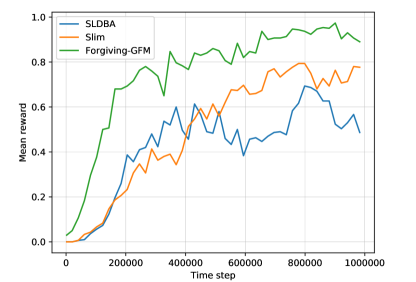
Figure 6: Learning curves

Training of the continuous-statespace model employed Proximal Policy Optimization (PPO) [30] as implemented in OpenAI Baselines [6]. Most training parameters were left unmodified from their defaults. This includes using the Adam optimizer [16] with a learning rate of $3\times 10^{-4}$, a discount factor $\gamma=0.99$, and $K=4$ epochs of optimization per iteration. Each iteration consisted of 2048 steps sampled from 12 parallel environments. The clipping parameter was changed to $\epsilon=0.1$. We also modified the default network architecture to contain two hidden layers with 128 neurons per layer. Each hidden layer was followed by a hyperbolic tangent activation. The training parameters remained the same for each automaton used in our experiment.

Figure 6 shows the learning curves for the three automata averaged over three runs. They underline the importance of choosing the right automaton in RL.

6 Conclusion

We have defined the class of automata that are good for MDPs—nondeterministic automata that can be used for the analysis of MDPs—and shown it to be closed under different simulation relations. This has multiple favorable implications for model checking and reinforcement learning. Closure under classic simulation opens a rich toolbox of statespace reduction techniques that come in handy to push the boundary of analysis techniques, while the more powerful (and more expensive) AEC simulation has promise to identify source automata that happen to be good for MDPs. Using standard and (very basic) AEC simulation, we only failed to establish the good for MDPs property for the NBAs created for $570$ of $685$ random LTL examples that are not expressible as DBAs, $69$ of them due to timeout.

The wider class of GFM automata also shows promise: the slim automata we have defined to tame the branching degree while retaining the desirable Büchi condition for reinforcement learning are able to compete even against optimized SLDBAs.

As outlined in Section 5.2, a low branching degree, cautiousness, and forgiveness make automata particularly well-suited for learning. A low branching degree is the easiest among them to quantify, and the slim automata tick this box perfectly. We have also argued that they are contributing towards cautiousness. For forgiveness, on the other hand, we had to hand-craft automata that satisfy this property. From a practical point of view, much of the power of this new approach is in harnessing the power of simulation for learning, and forgiveness is closely related to simulation.

The natural follow-up research is to tap the full potential of simulation-based statespace reduction instead of the limited version—which preserves limit determinism— that we have implemented. Besides using this to get the statespace small—useful for model checking—we will use simulation to construct forgiving automata, which is promising for reinforcement learning.

Appendix 0.A Reinforcement Learning Case Studies

We collect here the models and properties discussed in Section 5.2. The milk model, shown below as PRISM code [21], shows the effects of low branching degree. The property of interest is $\bigwedge_{0\leq i\leq 4}\operatorname{\mathsf{F}}\operatorname{\mathsf{G}}p_{i}$. The slim automaton has 275 states, while the SLDBA automaton has 7 states. Since the $p_{i}$’s are not mutually exclusive, the slim automaton needs a large number of states to limit the branching degree. Yet, for a fixed set of hyperparameter values, the agent learns the optimal policy with the slim automaton and fails to learn it with the SLDBA.

⬇

const int M = 12;

module m

b $\colon$ [0..M] init M;

[a] true $\rightarrow$ (b’ = b > 0 ? b-1 $\colon$ b);

endmodule

label ”p0” = b > 0;

label ”p1” = b > 1;

label ”p2” = b > 2;

label ”p3” = b > 3;

label ”p4” = b = 0;

The oddChocolates model shows the benefits of cautiousness in resolving nondeterminism. The property is $\operatorname{\mathsf{F}}\operatorname{\mathsf{G}}\mathtt{odd}$. The slim automaton has 4 states and is limit-deterministic, while the usual SLDBA, optimized for size, has 3 states. The extra state produced by the breakpoint construction allows the slim automaton to jump to the accepting part only after seeing two consecutive “odd” states. As a result, for a fixed set of hyperparameter values, and the tool Mungojerrie [13], the agent reliably learns an optimal policy, unlike the case of the smaller SLDBA automaton.

⬇

const int N = 5;

const int M = 12;

module pluck

b0 $\colon$ [0..M] init M;

b1 $\colon$ [0..M] init M;

b2 $\colon$ [0..M] init M;

b3 $\colon$ [0..M] init M;

b4 $\colon$ [0..M] init M;

[a0] true $\rightarrow$ (b0’ = b0 > 0 ? b0-1 $\colon$ b0);

[a1] true $\rightarrow$ (b1’ = b1 > 0 ? b1-1 $\colon$ b1);

[a2] true $\rightarrow$ (b2’ = b2 > 0 ? b2-1 $\colon$ b2);

[a3] true $\rightarrow$ (b3’ = b3 > 0 ? b3-1 $\colon$ b3);

[a4] true $\rightarrow$ (b4’ = b4 > 0 ? b4-1 $\colon$ b4);

endmodule

label ”odd” = mod(b0+b1+b2+b3+b4,2) = 1;

The forgiveness model below illustrates the effects of forgiveness. Its main feature is to produce, while in its transient states, deceiving hints for the learner. Two automata for $(\operatorname{\mathsf{F}}\operatorname{\mathsf{G}}x)\vee(\operatorname{\mathsf{G}}\operatorname{\mathsf{F}}y)$ are shown in Figure 5. The slim automaton produced by the breakpoint construction is not limit-deterministic. It accepts behaviors that satisfy $\operatorname{\mathsf{G}}\operatorname{\mathsf{F}}y$ before (irreversibly) jumping and behaviors that satisfy $\operatorname{\mathsf{F}}\operatorname{\mathsf{G}}x$ after jumping. Therefore the agent can recover from mistakenly believing that an MDP run will satisfy $\operatorname{\mathsf{G}}\operatorname{\mathsf{F}}y$, while it ends up satisfying $\operatorname{\mathsf{F}}\operatorname{\mathsf{G}}x$, but not vice versa. Accordingly, the results with the slim automaton are in between those of the two automata of Figure 5.

⬇

const double p = 1/2;

const double q = 0.1;

const int N = 5;

module m

s $\colon$ [0..7] init 0;

d $\colon$ [0..N] init N;

[a] s=0 $\rightarrow$ p $\colon$ (s’=1) + (1-p) $\colon$ (s’=2);

[b] s=0 $\rightarrow$ p $\colon$ (s’=2) + (1-p) $\colon$ (s’=3);

[c] (s=1 $\lor$ s=2) $\land$ d > 0 $\rightarrow$ q $\colon$ (d’=d-1) + (1-q) $\colon$ true;

[c] (s=1 $\lor$ s=2) $\land$ d = 0 $\rightarrow$ (s’=s+3);

[c] s=3 $\rightarrow$ true;

[a] s=4 $\lor$ s=5 $\rightarrow$ q $\colon$ (s’=s+2) + (1-q) $\colon$ true;

[b] s=4 $\lor$ s=5 $\rightarrow$ true;

[c] s=6 $\lor$ s=7 $\rightarrow$ (s’=s-2);

endmodule

label ”x” = s=1 $\lor$ s=5;

label ”y” = s=2 $\lor$ s=6;

Appendix 0.B Proving Simulation

0.B.1 Classic Simulation

In the following, we discuss how we can prove that a given Büchi automaton ${\cal D}=\langle\Sigma,Q_{\cal D},Q_{{\cal D},0},\Delta_{\cal D},\Gamma_{\cal D}\rangle$ (duplicator) simulates a Büchi automaton ${\cal S}=\langle\Sigma,Q_{\cal S},Q_{{\cal S},0},\Delta_{\cal S},\Gamma_{\cal S}\rangle$ (spoiler). The basic idea is to construct a parity game $\cal G$ such that the even player wins if and only if the simulation holds. The construction of the game is fairly standard and closely follows the outline from Subsection  3.1.

In our notion, we define parity games as follows.

Definition 2

A transition-labelled maximum parity game is a tuple

$${\cal P}=\langle Q_{0},Q_{1},\Delta,c\rangle$$

where for $Q=Q_{0}\cup Q_{1}$ we have

• $Q_{0}\cap Q_{1}=\emptyset$,

• $\Delta\subseteq Q\times Q$,

• $c\colon Q\times Q\rightharpoonup\mathbb{N}$ where $\mathit{Dom}(c)=\Delta$.

An infinite play is an infinite sequence $p=q_{0}q_{1}\ldots\in Q^{\omega}$ such for for all $i\geq 0$ it is $(q_{i},q_{i+1})\in\Delta$. An infinite play $p$ is winning if the highest colour which appears infinitely often is even, that is $\max\left\{c^{\prime}\mid\forall i\geq 0\exists j\geq i.\ c^{\prime}=c(q_{j},q_{j+1})\right\}\ \mathrm{mod}\ 2=0$. By $\mathrm{infplays}({\cal P})$ we denote the set of all infinite plays of ${\cal P}$. A finite play is a finite sequence $p=q_{0}q_{1}\ldots q_{n}\in Q^{*}$ such for for all $i,0\leq i\leq n-1$ it is $(q_{i},q_{i+1})\in\Delta$. By $\mathrm{finplays}_{i}({\cal P})$ we denote the set of all finite plays $p$ of ${\cal P}$ such that $q_{n}\in Q_{i}$ for $i\in\{0,1\}$. A strategy for player $i$ is a function $f_{i}\colon\mathrm{finplays}_{i}({\cal P})\to Q$ such that for $p=q_{0}q_{1}\ldots q_{n}$ we have $(q_{n},f(p))\in\Delta$. Given a pair of a player $0$ and player $1$ strategies $\langle f_{0},f_{1}\rangle$, the induced play starting from state $q$ is $p=q_{0}q_{1}q_{2}\ldots$ where $q_{0}=q$ and for all $k\geq 0$ we have $q_{k+1}=f_{i}(q_{k})$ where $q_{k}\in\Delta_{i}$. A player $0$ strategy $f_{0}$ is winning in a state $q$ if for every player $1$ strategy $f_{1}$ the induced play is winning.

Note that here colours are attached to transitions. This change is only for technical convenience, because colours naturally occur on the edges rather than states of the games we construct. Models of this type can either be transformed to state-labelled parity games or solved by slightly adapted versions of existing algorithms.

The parity game we construct is then as follows:

Definition 3

Consider two Büchi automata ${\cal S}=\langle\Sigma,Q_{\cal S},Q_{{\cal S},0},\Delta_{\cal S},\Gamma_{\cal S}\rangle$ and ${\cal D}=\langle\Sigma,Q_{\cal D},Q_{{\cal D},0},\Delta_{\cal D},\Gamma_{\cal D}\rangle$. The classical simulation parity game ${\cal P}_{{\cal S},{\cal D},\mathrm{sim0}}$ is defined as

$${\cal P}_{{\cal S},{\cal D},\mathrm{sim0}}=\langle Q_{0},Q_{1},\Delta,c\rangle$$

where

• $Q_{0}=Q_{\cal S}\times Q_{\cal D}\times\Sigma$,

• $Q_{1}=Q_{\cal S}\times Q_{\cal D}$,

• $\Delta=\Delta_{1}\cup\Delta_{0}$ where

• $\Delta_{0}=\left\{((q_{\cal S},q_{\cal D},a),(q_{\cal S},q_{\cal D}^{\prime}))\mid(q_{\cal D},a,q_{\cal D}^{\prime})\in\Delta_{\cal D}\right\}$

• $c((q_{\cal S},q_{\cal D},a),(q_{\cal S},q_{\cal D}^{\prime}))=\begin{cases}2&(q_{\cal D},a,q_{\cal D}^{\prime})\in\Gamma_{\cal D}\\ 0&\text{else}\end{cases}$

• $\Delta_{1}=\left\{((q_{\cal S},q_{\cal D}),(q_{\cal S}^{\prime},q_{\cal D},a))\mid(q_{\cal S},a,q_{\cal S}^{\prime})\in\Delta_{\cal S}\right\}$

• $c((q_{\cal S},q_{\cal D}),(q_{\cal S}^{\prime},q_{\cal D},a))=\begin{cases}1&(q_{\cal S},a,q_{\cal S}^{\prime})\in\Gamma_{\cal S}\\ 0&\text{else}\end{cases}$

The states $Q_{1}=Q_{\cal S}\times Q_{\cal D}$ are the states controlled by the spoiler. A state $(q_{\cal S},q_{\cal D})$ represents the situation where the spoiler is in state $q_{\cal S}$ and the duplicator is in state $q_{\cal D}$. States $Q_{0}=Q_{\cal S}\times Q_{\cal D}\times\Sigma$ are controlled by the duplicator. A state $(q_{\cal S},q_{\cal D},a)$ represents the situation where the spoiler has chosen a transition with label $a$ and has moved to state $q_{\cal S}$ then; the component $a$ has to be included in the state description, because the duplicator has to react with a transition with the same label as the one chosen by the spoiler. The transitions of $\Delta_{1}$ are the ones of the spoiler. The spoiler can choose any input $a$ from its current state $q_{\cal S}$ and then move to its successor state $q_{\cal S}^{\prime}$ if $(q_{\cal S},a,q_{\cal S}^{\prime})$ is a valid transition in the spoiler automaton. If this transition is an accepting transition (in the spoiler automaton), then it will have colour $1$, otherwise $0$. The transitions of $\Delta_{0}$ are the ones of the duplicator. In a state $(q_{\cal S},q_{\cal D},a)$, the duplicator has to choose a transition (in the Büchi automaton) labelled with $a$, because this was the choice of input of the spoiler. If this transition is accepting, the transition in the game will have label $2$, otherwise it will have label $0$.

Now, a play of the constructed parity game exactly describes a simulation game of Subsection 3.1. Also, the play is winning if and only if the simulation game is winning: If the duplicator wins the game, then either a) neither the spoiler nor the duplicator have infinitely many accepting transitions or b) the duplicator has infinitely many accepting transitions. In case a), the resulting colour of the play will be $0$. In case b), the resulting colour will be $2$. In both cases, it is even and the even player wins. Because of this, we have the following:

Lemma 2

Consider Büchi automata ${\cal S}=\langle\Sigma,Q_{\cal S},Q_{{\cal S},0},\Delta_{\cal S},\Gamma_{\cal S}\rangle$ and ${\cal D}=\langle\Sigma,Q_{\cal D},Q_{{\cal D},0},\Delta_{\cal D},\Gamma_{\cal D}\rangle$ and the classical simulation parity game ${\cal P}_{{\cal S},{\cal D}}$. Assume that for all $q_{\cal S}\in Q_{{\cal S},0}$ we have $q_{\cal D}\in Q_{{\cal D},0}$ such that $(q_{\cal S},q_{\cal D})$ is a winning state in the parity game. Then ${\cal D}$ simulates ${\cal S}$. Otherwise, ${\cal D}$ does not simulate ${\cal S}$.

To use the above lemma to show that simulation holds, the usual algorithms for solving parity games can be used (with a slight adaption to take into account the fact that the edges are labelled with a parity rather than the states). We have implemented a variation of the McNaughton algorithm [22]. Note that the parity games we construct have no more than three colours, for which a specialised algorithms exists [10]. However, because in our experience it always took much more time to construct the parity game than to solve this, we did not apply this specialised algorithm so far.

0.B.2 AEC Simulation

Classic simulation is not required to preserve good for MDP-ness, and the above parity game might fail to demonstrate a good for MDP property. In Subsection 4, we have discussed of how the simulation can be refined such that more automata can be proven to be sufficiently similar for our purpose (AEC simulation). In the next definition, we force the spoiler to choose a transition which is to be repeated infinitely often.

Definition 4

Consider two Büchi automata ${\cal S}=\langle\Sigma,Q_{\cal S},Q_{{\cal S},0},\Delta_{\cal S},\Gamma_{\cal S}\rangle$ and ${\cal D}=\langle\Sigma,Q_{\cal D},Q_{{\cal D},0},\Delta_{\cal D},\Gamma_{\cal D}\rangle$. The accepting transition simulation parity game ${\cal P}_{{\cal S},{\cal D},\mathrm{sim1}}$ is defined as

$${\cal P}_{{\cal S},{\cal D},\mathrm{sim1}}=\langle Q_{0},Q_{1},\Delta,c\rangle$$

where

• $Q_{0}=Q_{\cal S}\times Q_{\cal D}\times\Sigma\cup Q_{\cal S}\times Q_{\cal D}\times\Sigma\times(Q_{\cal S}\times\Sigma\times Q_{\cal S})$,

• $Q_{1}=Q_{\cal S}\times Q_{\cal D}\cup Q_{\cal S}\times Q_{\cal D}\times(Q_{\cal S}\times\Sigma\times Q_{\cal S})$,

• $\Delta=\Delta_{0,i}\cup\Delta_{1,i}\cup\Delta_{1,t}\cup\Delta_{0,f}\cup\Delta_{1,f}$ where

• $\Delta_{0,i}=\left\{((q_{\cal S},q_{\cal D},a),(q_{\cal S},q_{\cal D}^{\prime}))\mid(q_{\cal D},a,q_{\cal D}^{\prime})\in\Delta_{\cal D}\right\}$

• $c((q_{\cal S},q_{\cal D},a),(q_{\cal S},q_{\cal D}^{\prime}))=0$

• $\Delta_{1,i}=\left\{((q_{\cal S},q_{\cal D}),(q_{\cal S}^{\prime},q_{\cal D},a))\mid(q_{\cal S},a,q_{\cal S}^{\prime})\in\Delta_{\cal S}\right\}$,

• $c((q_{\cal S},q_{\cal D}),(q_{\cal S}^{\prime},q_{\cal D},a))=0$,

• $\Delta_{t}=\left\{((q_{\cal S},q_{\cal D}),(q_{\cal S}^{\prime},q_{\cal D},a,(q_{\cal S},a,q_{\cal S}^{\prime})))\mid(q_{\cal S},a,q_{\cal S}^{\prime})\in\Gamma_{\cal S}\right\}$

• $c((q_{\cal S},q_{\cal D}),(q_{\cal S}^{\prime},q_{\cal D},a,(q_{\cal S},a,q_{\cal S}^{\prime})))=0$,

• $\Delta_{0,f}=\left\{((q_{\cal S},q_{\cal D},a,e),(q_{\cal S},q_{\cal D}^{\prime},e))\mid(q_{\cal D},a,q_{\cal D}^{\prime})\in\Delta_{\cal D}\right\}$

• $c((q_{\cal S},q_{\cal D},a,e),(q_{\cal S},q_{\cal D}^{\prime},e))=\begin{cases}2&(q_{\cal D},a,q_{\cal D}^{\prime})\in\Gamma_{\cal D}\\ 0&\text{else}\end{cases}$

• $\Delta_{1,f}=\left\{((q_{\cal S},q_{\cal D},e),(q_{\cal S}^{\prime},q_{\cal D},a,e))\mid(q_{\cal S},a,q_{\cal S}^{\prime})\in\Delta_{\cal S}\right\}$

• $c((q_{\cal S},q_{\cal D},e),(q_{\cal S}^{\prime},q_{\cal D},a,e))=\begin{cases}1&(q_{\cal S},a,q_{\cal S}^{\prime})=e\\ 0&\text{else}\end{cases}$

For the two players, there are now two different types of states. The first type is like the state for the classical simulation parity game. The second type is extended by $(Q_{\cal S}\times\Sigma\times Q_{\cal S})$, such that it can store edges of the spoiler. There are now three types of transitions: $\Delta_{0,i}$ and $\Delta_{1,i}$ are similar to the ones of $\Delta_{0}$ and $\Delta_{0}$ of the classical simulation parity game. The difference is that the colour is always $0$. This implies that the spoiler cannot win by just using this type of transitions. Instead, she has to choose a transition of $\Delta_{t}$, which corresponds to choosing an edge to occur infinitely often. To reduce the size of the state-space and to ease definition, we restrict this choice such that it can only choose accepting edges, because it cannot win with non-accepting edges anyway. For the same reason, we only allow choosing the edge it just took. Transitions $\Delta_{0,f}$ and $\Delta_{1,f}$ correspond to the situation where the spoiler has already chosen an edge. Transitions of $\Delta_{0,f}$ are labelled with $2$ if they correspond to an accepting transition of the duplicator and $0$ otherwise. Transitions of $\Delta_{1,f}$ are labelled with $1$ if the edge is taken which the spoiler chose to appear infinitely often.

Lemma 3

Consider Büchi automata ${\cal S}=\langle\Sigma,Q_{\cal S},Q_{{\cal S},0},\Delta_{\cal S},\Gamma_{\cal S}\rangle$ and ${\cal D}=\langle\Sigma,Q_{\cal D},Q_{{\cal D},0},\Delta_{\cal D},\Gamma_{\cal D}\rangle$ and the accepting simulation parity game ${\cal P}_{{\cal S},{\cal D}}$. Assume that for all $q_{\cal S}\in Q_{{\cal S},0}$ we have $q_{\cal D}\in Q_{{\cal D},0}$ such that $(q_{\cal S},q_{\cal D})$ is a winning state in the parity game. Then ${\cal D}$ accepting transition simulates ${\cal S}$. Otherwise, ${\cal D}$ does not simulate ${\cal S}$.

Lemma 3 can be used to prove or disprove simulation in the same way as Lemma 2.

The simulation relation in which the duplicator is allowed to change the edge to be repeated infinitely often can be implemented in the following parity game:

Definition 5

Consider two Büchi automata ${\cal S}=\langle\Sigma,Q_{\cal S},Q_{{\cal S},0},\Delta_{\cal S},\Gamma_{\cal S}\rangle$ and ${\cal D}=\langle\Sigma,Q_{\cal D},Q_{{\cal D},0},\Delta_{\cal D},\Gamma_{\cal D}\rangle$. The accepting transition with update simulation parity game ${\cal P}_{{\cal S},{\cal D},\mathrm{sim2}}$ is defined as

$${\cal P}_{{\cal S},{\cal D},\mathrm{sim2}}=\langle Q_{0},Q_{1},\Delta,c\rangle$$

where

• $Q_{0}=Q_{\cal S}\times Q_{\cal D}\times\Sigma\cup Q_{\cal S}\times Q_{\cal D}\times(Q_{\cal S}\times\Sigma\times Q_{\cal S})\times(Q_{\cal S}\times\Sigma\times Q_{\cal S})$,

• $Q_{1}=Q_{\cal S}\times Q_{\cal D}\cup Q_{\cal S}\times Q_{\cal D}\times(Q_{\cal S}\times\Sigma\times Q_{\cal S})$,

• $\Delta=\Delta_{0,i}\cup\Delta_{1,i}\cup\Delta_{1,t}\cup\Delta_{0,f}\cup\Delta_{e}\cup\Delta_{1,f}$ where

• $\Delta_{0,i}=\left\{((q_{\cal S},q_{\cal D},a),(q_{\cal S},q_{\cal D}^{\prime}))\mid(q_{\cal D},a,q_{\cal D}^{\prime})\in\Delta_{\cal D}\right\}$

• $c((q_{\cal S},q_{\cal D},a),(q_{\cal S},q_{\cal D}^{\prime}))=0$,

• $\Delta_{1,i}=\left\{((q_{\cal S},q_{\cal D}),(q_{\cal S}^{\prime},q_{\cal D},a))\mid(q_{\cal S},a,q_{\cal S}^{\prime})\in\Delta_{\cal S}\right\}$,

• $c((q_{\cal S},q_{\cal D}),(q_{\cal S}^{\prime},q_{\cal D},a))=0$

• $\Delta_{t}=\left\{((q_{\cal S},q_{\cal D}),(q_{\cal S}^{\prime},q_{\cal D},(q_{\cal S},a,q_{\cal S}^{\prime}),(q_{\cal S},a,q_{\cal S}^{\prime})))\mid(q_{\cal S},a,q_{\cal S}^{\prime})\in\Gamma_{\cal S}\right\}$

• $c((q_{\cal S},q_{\cal D}),0,(q_{\cal S}^{\prime},q_{\cal D},(q_{\cal S},a,q_{\cal S}^{\prime}),(q_{\cal S},a,q_{\cal S}^{\prime})))=0$,

• $\Delta_{0,f}=\left\{((q_{\cal S},q_{\cal D},(\hat{q_{\cal S}},a,\hat{q_{\cal S}}),e),(q_{\cal S},q_{\cal D}^{\prime},e))\mid(q_{\cal D},a,q_{\cal D}^{\prime})\in\Delta_{\cal D}\right\}$,

• $c((q_{\cal S},q_{\cal D},(\hat{q_{\cal S}},a,\hat{q_{\cal S}}),e),(q_{\cal S},q_{\cal D}^{\prime},e))=\begin{cases}2&(q_{\cal D},a,q_{\cal D}^{\prime})\in\Gamma_{\cal D}\\ 0&\text{else}\end{cases}$

• $\Delta_{e}=\left\{((q_{\cal S},q_{\cal D},(\hat{q_{\cal S}},a,\hat{q_{\cal S}}),e),(q_{\cal S},q_{\cal D}^{\prime},(\hat{q_{\cal S}},a,\hat{q_{\cal S}})))\mid(q_{\cal D},a,q_{\cal D}^{\prime})\in\Delta_{\cal D}\right\}$,

• $c((q_{\cal S},q_{\cal D},(\hat{q_{\cal S}},a,\hat{q_{\cal S}}),e),(q_{\cal S},q_{\cal D}^{\prime},(\hat{q_{\cal S}},a,\hat{q_{\cal S}})))=\begin{cases}2&(q_{\cal D},a,q_{\cal D}^{\prime})\in\Gamma_{\cal D}\\ 0&\text{else}\\ \end{cases}$

• $\Delta_{1,f}=\left\{((q_{\cal S},q_{\cal D},e),(q_{\cal S}^{\prime},q_{\cal D},(q_{\cal S},a,q_{\cal S}^{\prime}),e))\mid(q_{\cal S},a,q_{\cal S}^{\prime})\in\Delta_{\cal S}\right\}$,

• $c((q_{\cal S},q_{\cal D},e),(q_{\cal S}^{\prime},q_{\cal D},(q_{\cal S},a,q_{\cal S}^{\prime}),e))=\begin{cases}1&(q_{\cal S},a,q_{\cal S}^{\prime})=e\\ 0&\text{else}\end{cases}$

Compared to the accepting transition simulation parity game, we have changed the second type of duplicator states. The spoiler usually chooses an input, and then proceeds to a successor state with this input. Rather than just storing the input, we store the whole edge which the spoiler chose. This allows to change the edge which is expected to be seen infinitely often for the spoiler to win by using the transitions of type $\Delta_{e}$.

Lemma 4

Consider Büchi automata ${\cal S}=\langle\Sigma,Q_{\cal S},Q_{{\cal S},0},\Delta_{\cal S},\Gamma_{\cal S}\rangle$ and ${\cal D}=\langle\Sigma,Q_{\cal D},Q_{{\cal D},0},\Delta_{\cal D},\Gamma_{\cal D}\rangle$ and the accepting simulation with update parity game ${\cal P}_{{\cal S},{\cal D}}$. Assume that for all $q_{\cal S}\in Q_{{\cal S},0}$ we have $q_{\cal D}\in Q_{{\cal D},0}$ such that $(q_{\cal S},q_{\cal D})$ is a winning state in the parity game. Then ${\cal D}$ accepting transition with update simulates ${\cal S}$. Otherwise, ${\cal D}$ does not simulate ${\cal S}$.

Again, Lemma 4 can be used in the same way as Lemma 3.

References

- [1] T. Babiak, M. Křetínský, V. Rehák, and J. Strejcek. LTL to Büchi automata translation: Fast and more deterministic. In Tools and Algorithms for the Construction and Analysis of Systems, pages 95–109, 2012.
- [2] Ch. Baier and J.-P. Katoen. Principles of Model Checking. MIT Press, 2008.
- [3] C. Courcoubetis and M. Yannakakis. Verifying temporal properties of finite-state probabilistic programs. In Foundations of Computer Science, pages 338–345. IEEE, 1988.
- [4] C. Courcoubetis and M. Yannakakis. The complexity of probabilistic verification. J. ACM, 42(4):857–907, July 1995.
- [5] L. de Alfaro. Formal Verification of Probabilistic Systems. PhD thesis, Stanford University, 1998.
- [6] P. Dhariwal, Ch. Hesse, O. Klimov, A. Nichol, M. Plappert, A. Radford, J. Schulman, S. Sidor, Y. Wu, and P. Zhokhov. Openai baselines. https://github.com/openai/baselines, 2017.
- [7] D. L. Dill, A. J. Hu, and H. Wong-Toi. Checking for language inclusion using simulation relations. In Computer Aided Verification, pages 255–265, July 1991. LNCS 575.
- [8] A. Duret-Lutz, A. Lewkowicz, A. Fauchille, T. Michaud, E. Renault, and L. Xu. Spot 2.0 - A framework for LTL and -automata manipulation. In Automated Technology for Verification and Analysis, pages 122–129, 2016.
- [9] K. Etessami, T. Wilke, and R. A. Schuller. Fair simulation relations, parity games, and state space reduction for Büchi automata. SIAM J. Comput., 34(5):1159–1175, 2005.
- [10] K. Etessami, T. Wilke, and R. A. Schuller. Fair simulation relations, parity games, and state space reduction for Büchi automata. SIAM Journal of Computing, 34(5):1159–1175, 2005.
- [11] S. Gurumurthy, R. Bloem, and F. Somenzi. Fair simulation minimization. In Computer Aided Verification (CAV’02), pages 610–623, July 2002. LNCS 2404.
- [12] E. M. Hahn, G. Li, S. Schewe, A. Turrini, and L. Zhang. Lazy probabilistic model checking without determinisation. In Concurrency Theory, pages 354–367, 2015.
- [13] E. M. Hahn, M. Perez, S. Schewe, F. Somenzi, A. Trivedi, and D. Wojtczak. Omega-regular objectives in model-free reinforcement learning. In Tools and Algorithms for the Construction and Analysis of Systems, pages 395–412, 2019. LNCS 11427.
- [14] T. Henzinger, O. Kupferman, and S. Rajamani. Fair simulation. In Concurrency Theory, pages 273–287, 1997. LNCS 1243.
- [15] T. A. Henzinger and N. Piterman. Solving games without determinization. In Computer Science Logic, pages 394–409, September 2006. LNCS 4207.
- [16] Diederik P. Kingma and Jimmy Ba. Adam: A method for stochastic optimization, 2014.
- [17] D. Kini and M. Viswanathan. Optimal translation of LTL to limit deterministic automata. In Tools and Algorithms for the Construction and Analysis of Systems, pages 113–129, 2017.
- [18] J. Klein, D. Müller, Ch. Baier, and S. Klüppelholz. Are good-for-games automata good for probabilistic model checking? In Language and Automata Theory and Applications, pages 453–465, 2014.
- [19] J. Křetínský, T. Meggendorfer, S. Sickert, and Ch. Ziegler. Rabinizer 4: from LTL to your favourite deterministic automaton. In Computer Aided Verification, pages 567–577. Springer, 2018.
- [20] J. Křetínský, T. Meggendorfer, and S. Sickert. Owl: A library for -words, automata, and LTL. In Automated Technology for Verification and Analysis, pages 543–550, 2018.
- [21] M. Kwiatkowska, G. Norman, and D. Parker. PRISM 4.0: Verification of probabilistic real-time systems. In Computer Aided Verification, pages 585–591, July 2011. LNCS 6806.
- [22] R. McNaughton. Testing and generating infinite sequences by a finite automaton. Information and Control, 9:521–530, 1966.
- [23] R. Milner. An algebraic definition of simulation between programs. Int. Joint Conf. on Artificial Intelligence, pages 481–489, 1971.
- [24] N. Piterman. From deterministic Büchi and Streett automata to deterministic parity automata. Logical Methods in Computer Science, 3(3):1–21, 2007.
- [25] M. L. Puterman. Markov Decision Processes: Discrete Stochastic Dynamic Programming. John Wiley & Sons, New York, NY, USA, 1994.
- [26] S. Safra. Complexity of Automata on Infinite Objects. PhD thesis, The Weizmann Institute of Science, March 1989.
- [27] S. Schewe. Beyond hyper-minimisation—minimising DBAs and DPAs is NP-complete. In Foundations of Software Technology and Theoretical Computer Science, FSTTCS, pages 400–411, 2010.
- [28] S. Schewe and T. Varghese. Tight bounds for the determinisation and complementation of generalised Büchi automata. In Automated Technology for Verification and Analysis, pages 42–56, 2012.
- [29] S. Schewe and T. Varghese. Determinising parity automata. In Mathematical Foundations of Computer Science, pages 486–498, 2014.
- [30] J. Schulman, F. Wolski, P. Dhariwal, A. Radford, and O. Klimov. Proximal policy optimization algorithms. CoRR, abs/1707.06347, 2017.
- [31] S. Sickert, J. Esparza, S. Jaax, and J. Křetínský. Limit-deterministic Büchi automata for linear temporal logic. In Computer Aided Verification, pages 312–332, 2016. LNCS 9780.
- [32] S. Sickert and J. Křetínský. MoChiBA: Probabilistic LTL model checking using limit-deterministic Büchi automata. In Automated Technology for Verification and Analysis, pages 130–137, 2016.
- [33] F. Somenzi and R. Bloem. Efficient Büchi automata from LTL formulae. In Computer Aided Verification, pages 248–263, July 2000. LNCS 1855.
- [34] M.-H. Tsai, S. Fogarty, M. Y. Vardi, and Y.-K. Tsay. State of Büchi complementation. Logical Mehods in Computer Science, 10(4), 2014.
- [35] M.-H. Tsai, Y.-K. Tsay, and Y.-S. Hwang. GOAL for games, omega-automata, and logics. In Computer Aided Verification, pages 883–889, 2013.
- [36] M. Y. Vardi. Automatic verification of probabilistic concurrent finite state programs. In Foundations of Computer Science, pages 327–338, 1985.