Design-adherent estimators for network surveys

Abstract

Network surveys of key populations at risk for HIV are an essential part of the effort to understand how the epidemic spreads and how it can be prevented. Estimation of population values from the sample data has been probematical, however, because the link-tracing of the network surveys includes different people in the sample with unequal probabilities, and these inclusion probabilities have to be estimated accurately to avoid large biases in survey estimates. A new approach to estimation is introduced here, based on resampling the sample network many times using a design that adheres to main features of the design used in the field. These features include network link tracing, branching, and without-replacement sampling. The frequency that a person is included in the resamples is used to estimate the inclusion probability for each person in the original sample, and these estimates of inclusion probabilities are used in an unequal-probability estimator. In simulations using a population of drug users, sex workers, and their partners for which the actual values of population characteristics are known, the design-adherent estimation approach increases the accuracy of estimates of population quantities, largely by eliminating most of the biases.

1 Introduction

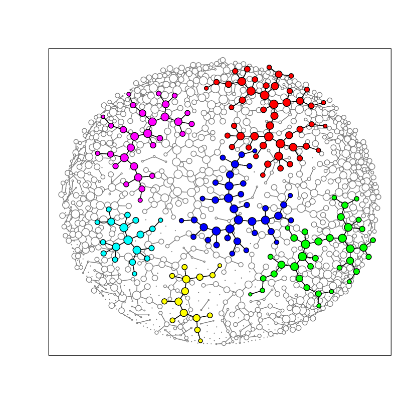
Figure 1: A network sample of 1200 people from a high-risk hidden population. Some sample components are highlighted. The network sample is resampled many times using a network sampling design that adheres closely to the original survey design. The frequency that a person is included in the resamples (circle diameter) is used to estimate the person’s inclusion probability in the original sample. These estimated inclusion probabilities enable estimates of hidden-population characteristics.

Network sample surveys have become an essential part of the effort to understand and alleviate the HIV epidemic worldwide. Much of the spread of the epidemic is over sexual and drug-using connections among hidden or hard-to-access populations. Network surveys that follow social links between members of the hidden population are effective and often the only feasible way to reach into the key populations most at risk for HIV. Estimation of the characteristics of the key population from the survey data has been problematical because the link-tracing designs find different members of the population with unequal probabilities depending on network connection patterns. The core problem of network sampling is to estimate the inclusion probabilities of the actual design accurately.

A new approach to estimation for network surveys is described in this report. The idea underlying the method is to select many resamples from the sample network using a design that adheres closely to features of the actual design used in selecting the sample from the hidden population. For each person in the sample, the inclusion frequency of that person in the resamples is used as an estimate of that person’s relative inclusion probability in the original sample. The estimated inclusion probabilities are then used to estimate population characteristics and calculate confidence intervals.

Figure 1 shows a sample of 1200 people selected by Respondent-Driven Sampling (RDS) in which each respondent has been given up to 3 coupons to recruit some of his or her partners into the sample. Several sample components are highlighted. Each of these components was started from a single seed. Links were traced to add additional people to the sample. A person could not be recruited more than once so the sampling is without-replacement.

If instead we used a Snowball (SB) design allowing unlimited recruitments or up to some high maximum like 15, the sample would tend to have larger components and much more branching. With either of these designs, the sample is a network tree, with only a single path from one individual to another that does no backtracking. Each individual may have more links than are found in the sampling, because of the limits on recruitment and the chances that a recruiting attempt is successful or not.

In some surveys (termed RDS+ or SB+ here), extra social network interviews or relationship matching determine additional links between sample members. So a person in the (red) component at the top of the figure might have an additional link, that was not used in recruiting, to another person in that or another component. With the extra links the sample, like the population, would not be a tree but a more general network structure containing cycles or multiple paths between individuals.

A random walk design, which allows no branching, would produce a sample very different from Figure 1. Each respondent would be given exactly one coupon, to select up to one partner, and that partner would in turn be given one coupon, and so on. The sample components would look like crooked stems, rather than trees. Random walk designs are seldom if ever used in actual network surveys. But the theoretical inclusion probabilities of a with-replacement random walk is used as the basis for currently used estimators. The discrepancy between the assumed theoretical design and the actual survey design used gives rise to the statistical problems of the currently used estimators.

The branching, without-replacement designs have several advantages over a non-branching or with-replacement design. The without-replacement sampling means that each selection is a new node, not already selected, and so the number of distinct units in the sample grows steadily. The branching allows the sample to spread and grow rapidly when a link-rich, highly connected area of the social network is encountered.

An under-appreciated feature of the branching, without-replacement network sampling designs such as RDS and SB designs is their ability to self-allocate, so that proportionally more sampling effort is made in the highly connected parts of the hidden population. Suppose that in the hidden population are two separate components, so that no path of links leads from one to the other, and that one of the components is more densely connected, having more links and paths than the other. If an equal number of random-walk seeds are placed in each component, after any number of steps there will still be the equal numbers of sample nodes selected in each component. With a branching design, if equal numbers of seeds are selected in each component, there will after several steps be many more sample nodes in the component that has the more links and connections, because at any time there are more links out from the sample that can be followed, so probabilistically more of the selections will be made in the more densely-connected component. This will happen naturally even when the recruiting of new sample members is done by the hidden-population respondents. This self-allocation with the branching, without-replacement design serves also to make the designs effective at finding densely connected centers in the network, and once the sample finds those the recruitments spread outwork in all directions from those centers.

How the estimation method works

In traditional survey sampling with unequal probabilities of inclusion for different people, typical estimators divide an observed value $y_{i}$ for the $i$th person by the inclusion probability $\pi_{i}$ that person. The variable of interest $y_{i}$ might be 1 if the person tests positive for a virus and 0 otherwise, or might be the number of partners that person reports having. The inverse-weighting gives an unbiased or low-bias estimate of the population proportion or mean of that variable. In network surveys the inclusion probabilities are unknown so they need to be estimated.

The estimators described in this report estimate the inclusion probability of each person in the sample by selecting many resamples from the network sample data using a design that adheres in key features to the actual survey design used to find the sample. In particular, the resampling design is a link-tracing design done without-replacement and with branching, as was the original design. The frequency $f_{i}$ with which an individual is included in the resamples is used as an estimate of that person’s inclusion probability $\pi_{i}$.

What we do is select $T$ resamples $S_{1},S_{2},...,S_{T}$ from the sample network data. There are two aproaches to selecting the sequence of resamples. In the repeated-samples approach each resample is selected independently from seeds and progresses step-by-step to target resample size independently of every other resample, so we get a collection of independent resamples. in the sampling-process approach each resample $S_{t}$ is selected from the resample $S_{t-1}$ just before it by randomly tracing a few links out and randomly removing a few nodes from the previous resample and using a small rate of re-seeding so we do not get locked out of any component by chance. It is this Markov resampling process approach that we use for the simulations in this paper because it is so computationally efficient.

For an individual $i$ in the original sample, there is a sequence of zeros and ones $Z_{i1},Z_{i2},...,Z_{iT}$, where $Z_{t}$ is 1 if that person is included in resample $S_{t}$ and is 0 if the person is not included in that resample. The inclusion frequency for person $i$ is

$$f_{i}=\frac{1}{T}\left(Z_{i1}+Z_{i2}+...+Z_{iT}\right)$$ (1)

In Figure 1 the circle representing individual $i$ in the sample is drawn with diameter proportional to the estimated inclusion probability $f_{i}$ of that individual. Individuals centrally located in sample components tend to have high values of $f_{i}$. That is because there are more paths, and paths of higher probability, leading the sample to those individuals. Also, individuals in larger components tend to have larger $f_{i}$ than individuals in smaller components, so that the method is estimating inclusion probability of an individual relative to all other sample units, not just those in the same component or local area or the sample This is because of the self-allocation of the branching design, even in the absence of re-seeding, to areas of the social network having more links and connected paths.

The estimator of the mean of a characteristic $y$ in the hidden population is then

$$\hat{\mu}_{f}=\frac{\sum(y_{i}/f_{i})}{\sum(1/f_{i})}$$ (2)

where each sum is over all the people in the sample. If the actual inclusion probabilities $\pi_{i}$ were known and replaced the $f_{i}$ in Equation 2 we would have the generalized unequal probability estimator $\hat{\mu}_{\pi}$ of Brewer Brewer (1963).

Why it works

To understand why the new method works, consider the two stages of sampling. The first-stage is the actual network sampling design by which the sample of people is selected from the hidden population. The second-stage design selects a resample of people from the network sample data, using a network sampling design similar to the one used in the real-world. The second-stage design, like the first, uses link-tracing, branches, and is done without-replacement. The second-stage design can not be exactly the same as the original design in every respect. For example the second-stage design has to use a smaller sample size than the original, because of the without-replacement sampling.

The probability that individual $i$ in the original sample is included in the resample will be called $\phi_{i}$. The ideal is to have the inclusion probability for a unit at the second stage, given the first stage sample, to be proportional to it’s inclusion probability in the original design. That is, $\phi_{i}=c\pi_{i}$, where $c$ is some constant, which does not need to be known.

Now let $\hat{\mu}_{\phi}$ be formula 2 with the exact resample probabilities $\phi_{i}$ replacing $f_{i}$. If $\phi_{i}=c\pi_{i}$, then $\hat{\mu}_{\phi}=\hat{\mu}_{\pi}$, because the constant of proportionality $c$ is in both the numerator and denominator of 2 and divides out of the estimator.

As the number of resamples $T$ gets large the inclusion frequencies $f_{i}$ converge in probability to the second-stage inclusion probabilities $\phi_{i}$. This is by the (weak) Law of Large Numbers for the independent resamples and by the Law of Large Numbers for Markov chains for the resampling process that traces a few and removes a few at each step.

It follows that if $\phi_{i}$ is proportional to $\pi_{i}$ then $\hat{\mu}_{f}$ converges in probability to $\hat{\mu}_{\phi}$. So if inclusion in the resample $\phi$ is proportional to inclusion in the original sample $\pi$ then the estimator we use here $\hat{\mu}_{f}$ converges to the general unequal probability estimator $\hat{\mu}_{\pi}$. Since the resampling is fast computationally, especially with the sampling process approach, we can readily select a lot of resamples, such as $T=10,000$ that we use in the simulations here, and higher values of $T$ like one million are still fast to compute.

The approximate part is in how close the second-stage inclusion probabilities $\phi_{i}$ are to proportionality with the first-stage inclusion probabilities $\phi_{i}$. This is why it is important that the resampling design adheres to the main features of the actual network design, such as network link tracing, branching, and without-replacement selections.

The use of the second stage sample is different here than in traditional two-stage sampling or in bootstrap methods. In each of those a given second-stage sample is used to make an estimate of a population value. If the sampling is with unequal probabilities at each stage, estimation of the population value from the second-stage sample requires dividing first by the second-stage inclusion probability $\phi_{i}$ to estimate what is in the first stage sample and then then by the first stage probability $\pi_{i}$. Here we use the second stage design solely to estimate its own inclusion probabilities and we construct the second-stage design to have those probabilities similar to the first-stage probabilities.

Background

Early uses of network sampling to find and study hidden populations in the typically used snowball sampling types of methods. Sample means and proportions were used to summarize data and implicitly to infer hidden population characteristics. Reviews of the early literature can be found in Spreen (1992), Heckathorn (1997), and Thompson and Collins (2002). Unbiased estimates of population values from relatively simple network sampling designs were obtained by Birnbaum and Sirken (1965) and Frank (1977). Frank and Snijders (1994) obtained design and model based estimates of the size of a hidden population of drug users with a one-wave snowball sample.

Starting with Heckathorn (1997), the methodology of Respondent-Driven-Sampling using dual-incentive coupons was introduced. Estimators for these designs based on random walk theory and assumptions of Markov transitions in the sampling between values of attribute variables of respondents were given in Salganik and Heckathorn (2004), Heckathorn (2007), and Volz and Heckathorn (2008). If a random walk with replacement is run in a network consisting of a single connected component, the long term frequency of inclusion of node $i$ is proportional to $d_{i}$. The simplest of these estimators divides observed value for an individual $i$ by degree $d_{i}$, the number of partners that person reports having. In relation to Equation 2 it could be denoted $\hat{\mu}_{d}$. It has the form of the general unequal probability estimator with $\pi_{i}$ approximated by $d_{i}$. It is commonly called the Volz-Heckathorn estimator (VH) or the Salganik-Volz-Heckathorn estimator. Following Goel and Salganik (2010), in this paper we refer to the VH also as the Current method, because it is the most commonly used in current practice and its assumptions are also made in the other commonly used variants. The estimator of Salganik and Heckathorn (2004) uses the VH estimator to estimate degree and for attribute variables adjusts that with proportions of sample recruitment links between and within the group with the attribute and the group without it. The adjustment is based on the additional assumption of Markov transitions between attribute states during the sampling.

The Successive Sampling (SS) estimator of Gile Gile (2011) adjusts the VH estimator for samples in which sample size $n$ is a substantial fraction of population size $N$. The improvement is based on the fact that the real sampling is done without replacement. As part of the procedure resampling with probability proportional to size among all units not already in the resample is used to estimate inclusion probability. In this way the use of resampling in Gile (2011), although it does not include link-tracing or branching, is similar in purpose to the use of the resampling in this paper. The measure of size of a unit in the successive sampling method is degree. When population size is large compared to sample size the SS esstimator defaults to the VH estimator.

Fellows Fellows (2018) introduces the Homophily Configuration Graph Estimator (HCG), which uses the attribute variable group membership in a manner similar to SH and adjusts for large sampling fraction with the SS method. When population size is large relative to sample size the HCG estimator defaults to the SH estimator for estimating the proportion with an attribute and to the VH for estimating mean degree.

Confidence interval methods commonly used with RDS designs include the Salganik bootstrap Salganik (2006) for SH and VH, the Gile SS bootstrap Gile (2011) for SS. A recent evaluation of these methods, for means of binary variables and using simulations based on a statistical network model fitted to RDS data is Spiller et al. (2017).

A different bootstrap approach for RDS data called a Tree Bootstrap is described in Baraff, McCormick and Raftery (2016) for making a confidence interval around the VH estimator. The bootstrap resamples are selected by first taking a random sample with replacement of the sample seeds. From each of those their sample tree is resampled, starting with the original seed and tracing links with replacement except not moving backwards to resample the recruiter at any step. With each resample, the VH estimator is calculated and the confidence interval is based on the quantiles of the distribution of the resample estimates. In making the bootstrap estimates of the population values, the necessity of dividing by second-stage (resample) inclusion probabilities is avoided by the equal-probabililty resampling of seeds. The Tree Bootstrap confidence intervals have good coverage probabilities but are wide compared to other methods. The need for wide intervals in order to have good coverage probability is not inherent to the Tree Bootstrap approach but is needed to overcome the bias offet of the VH estimator.

Estimation methods based on the VH estimator are based on node degrees. The SH estimator goes one step further into the sample network by using the proportion of links within a group to the number going out from that group. In contrast the methods in Thompson (2006), Crawford (2016), and Crawford, Wu and Heimer (2018) use the full sample network. Minimally, the sample network includes only those links within the sample that were used in recruitment, plus the counterpart edge in the other direction to make the link symmetric. The more full version of the sample network uses the set of all links that connect sample nodes.

RDS methods were evaluated in Goel and Salganik (2010) using a collection of real populations, of which Project 90 population is the most relevant to our interests here since it is an actual at-risk, hidden population in which link-tracing provides the only means of access and is not based in an institutional setting. They used simulations in which the RDS sampling was modeled as with-replacement, noting that in the field they were normally done without-replacement. They found the VH and SH estimators performed similarly and focused on study of the VH estimator, termed the Current Estimator. For the 13 attribute variables in the study their simulations found actual confidence interval coverages from 42% to 65% for nominally 95% confidence intervals. Design effects were found to be high with the RDS methods, reflecting the high mean squared errors.

RDS with the VH and SH estimators is examined in Gile and Handcock (2010) using simulation of the design with and without replacement and with branching in a variety of model-generated network populations. They found the VH estimator generally out-performed the SH estimator and that without-replacement designs generally resulted in lower variance and lower bias than with-replacement designs. They found biases in the estimates in many conditions. Between selection of seeds at random and with probability proportional to degree they found little difference in the resulting estimators, but stronger seed selection biases could affect the resulting properties.

An RDS design with supplement social network stucy, making the overall design RDS+ in the terminology of this paper, is used in Young, Rudolph and Havens (2018) to study a rural opioid user network in relation to HIV risk.

In this report the design-adherent estimators are evaluated with simulations using the reference Project 90 network data on a hidden population at risk for HIV Potterat, Rothenberg and Muth (1999). Some results of the present report were described in the earlier ArXiv working paper Thompson (2018).

2 Methods

Confidence intervals

A simple variance estimator to go with $\hat{\mu}_{f}$ is

$$\widehat{\textrm{v}ar}(\hat{\mu})=\frac{1}{n(n-1)}\sum_{s}\left(\frac{ny_{i}/f_{i}}{\sum_{s}(1/f_{i})}-\hat{\mu}_{f}\right)^{2}$$ (3)

The variance estimator is based on a simplified estimator for the variance of a Horvitz-Thompson estimator evaluated with simulations in Brewer and Hanif (1983), which has been modified here to apply to the generalized unequal probability estimator form of $\hat{\mu}_{f}$. An approximate $1-\alpha$ confidence interval is then calculated as $\hat{\mu}\pm z\sqrt{\widehat{\textrm{v}ar}(\hat{\mu})}$, with $z$ the $1-\alpha/2$ quantile from the standard Normal distribution. A different variance estimator was used for these estimators in the working paper Thompson (2018). In the simulations here the estimator above gives a slightly higher average confidence interval coverage probability.

Simulations

The simulations were done using the entire network data set of 5492 people and 21,644 links from the Colorado Springs Project 90 study on the heterosexual spread of HIV Potterat, Rothenberg and Muth (1999). The same data set was used in simulations in Goel and Salganik (2010), Baraff, McCormick and Raftery (2016), and Fellows (2018). The data are available to researchers (https://opr.princeton.edu/archive/p90/). The links combine drug, sexual, and social relationships.

For each of the four designs, 1000 samples of target size $n=1200$ were selected from the 5492 study population. In RDS and RDS+, 3 coupons were given to each respondent (fewer if the respondent had fewer than 3 partners). In SB and SB+, the coupon maximum was 15. Coupons had an expiration date 28 days from issue. Seeds (240 or 20% of $n$) were selected at random. The resampling process, like the original design, used link-tracing, branching, and without-replacement sampling. No coupons were used in the resampling process, so that the same resampling design was used for each of the four original designs. As can be seen from the RDS sample in Figure 1 where each respondent was given no more than 3 coupons with which to, a without-replacement resample can at no point branch more than 3 in any case, or up to 4 branches from a re-seed. For each of the 1000 samples, the design-adherent estimator was calculated by selecting $T=10,000$ resamples each of target size 400 and averaging the inclusion indicators for each of the 1200 sample people, giving the frequencies $f_{i}$ to calculate the estimate $\hat{\mu}_{f}$.

Resampling process versus independent resamples

Selecting many samples from the sample network data to estimate the inclusion probabilities can be done with either independent resamples from seeds to target sample size or using the Markov chain resampling process. The resampling processes method is much faster computationally and is the approach that was used in the simulations.

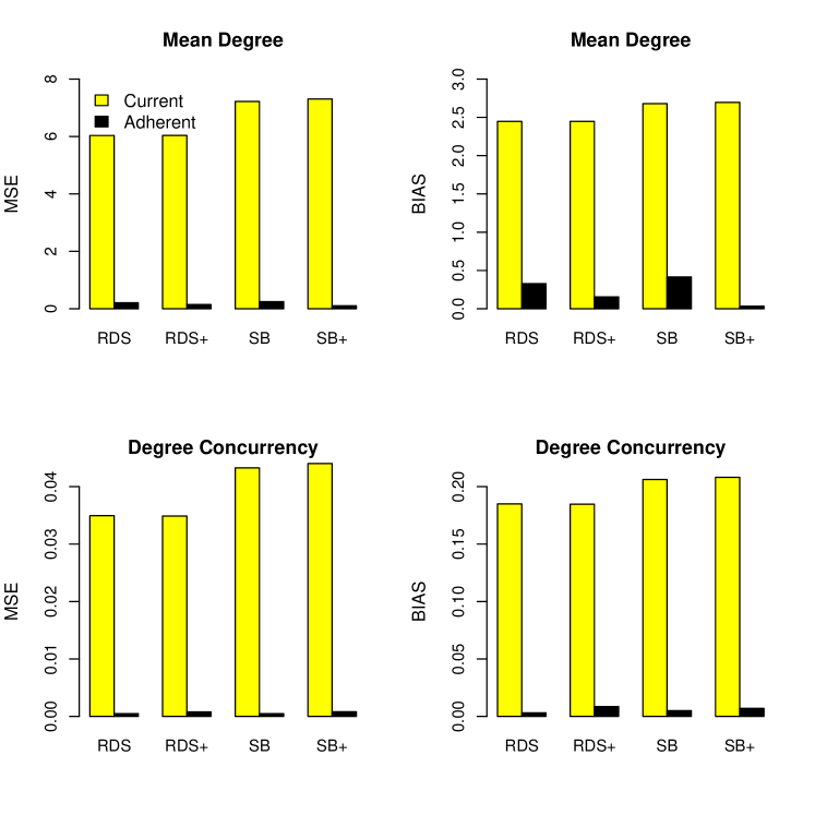
Figure 2: The mean square error (left) and bias (right) of the adherent estimator (black) is lower than that of the current estimator (yellow) for estimating mean degree (top) and degree concurrency—proportion of people with two or more partners (bottom) for each of four network sampling designs. The design RDS restricts branching to limiting coupons to a maximum of 3. The snowball (SB) design gives respondents as many coupons as their number of partners, up to a maximum of 15, allowing almost unlimited branching as the sample is selected. The “+” version of each design obtains additional social network information from the given set of sample members.

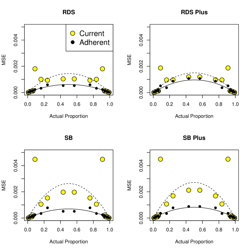
Figure 3: Mean squared error of the estimate of population proportion for each of 13 individual attributes. The adherent estimator (black) is compared to the current estimator (yellow). To help see the pattern, the estimate of the compliment of each attribute is shown. The compliment of sex work client, for example, is not-client. A parabolic curve is fitted by weighted least squares to the MSEs of the adherent estimator (solid line) and the current estimator (dashed line). The adherent estimator MSEs have a lower fitted curve with a better fit with each design.

		RDS	RDS Plus	SB	SB Plus
1	degree	0.77	0.86	0.72	0.92
2	nonwhite	0.95	0.86	0.92	0.88
3	female	0.98	0.99	0.99	0.99
4	sex worker	0.95	0.92	0.95	0.94
5	procuring agent	0.90	0.69	0.95	0.85
6	sex-worker client	0.95	0.72	0.96	0.79
7	dealer	0.95	0.78	0.94	0.85
8	cook	0.78	0.65	0.79	0.67
9	thief	0.94	0.65	0.93	0.71
10	retired	0.93	0.84	0.93	0.84
11	homemaker	0.94	0.93	0.93	0.91
12	disabled	0.94	0.89	0.94	0.89
13	unemployed	0.95	0.94	0.95	0.94
14	homeless	0.88	0.67	0.86	0.67
15	degree concurrency	1.00	1.00	1.00	1.00

Table 1: Confidence Interval Coverage Probabilities

3 Results

Two link-related quantities of interest in studies of key populations at risk for HIV and other infectious diseases are mean degree and degree concurrency. Mean degree is the average number of partners per person in the population. Degree concurrency is the proportion of people in the population who have two or more partners. A high number for either of these is an indication that an epidemic could spread rapidly in the population once it starts there.

The top two plots in Figure 2 are on estimating mean degree. In each plot the four designs, from left to right, are standard Respondent Driven Sampling (RDS), enhanced Respondent Driven Sampling (RDS+), Snowball Sampling (SB), and enhanced Snowball Sampling (SB+). Respondent Driven Sampling limits each recruiter to 3 coupons, which which they can recruit up to 3 of their partners into the study. Snowball Sampling here has a coupon limit of 15.

In Figure 2 the top left plot shows the mean squared error for the current estimator (yellow bar). The black bar next to it is the mean square error for the design-adherent estimator. Starting with the left-most pair of bars, the mean square error for the current method (VH estimator) for RDS sampling is 6.03. The mean square error for the design-adherent estimator, in which the estimation takes into account the branching and without replacement in the sampling, the mean square error is 0.21. The reduction in mean squared error comes largely from eliminating most of the bias, as shown in the top right plot of Figure 2. The actual mean degree in the Project 90 study population is 7.89 partners per person. The current estimator underestimates this on average by 2.45 partners (yellow bar). The adherent estimator overestimates by 0.32 partners on average (black bar).

To understand better what is happening in the estimation we will look more closely at this one case before going on to the overall pattern in all the results. Mean squared error of an estimator is related to its bias and standard deviation by MSE = (Bias)² + (SD)². Here the MSE. Here the squared bias 5.99 accounts for almost all of the MSE 6.03. The adherent estimator reduces the squared bias to 0.11 which is about half of its MSE. So the efficiency gain is due to the elimination of most of the bias. The reduction in bias is obtained by the more accurate estimates of inclusion probabilities using a the resampling design that adheres to the the branching and without-replacement features of the actual survey design, and using the sample network recruitment data instead of assumptions about the hidden population network.

For estimating mean degree, with the RDS design the relative efficiency of the design-adherent method, (MSE($\hat{\mu}$)/MSE($\hat{\mu}_{d}$), is 29. So with the same design, adhering to design features in estimation reduces the mean squared error to 1/29 that of the current method. With the other designs, the efficiency gains of the adherent estimation are 41 for RDS Plus, 29 for SB, and 68 for SB plus. In each case this is accomplished through the reduction in bias with the design-adherent method.

For estimating the proportion of people in the population with two or more partners (degree concurrency), the relative efficiencies of the adherent estimators compared to the current estimators are 72 for RDS, 44 for RDS Plus, 92 for SB, and 55 for SB Plus. Once again the reduction in MSE is explained by the reduction in bias.

The Project 90 node data includes 13 individual attribute variables such as sex worker, client of sex worker, or unemployed. These are variables 2 through 14 in Table 1. For an individual, the value is 1 if the individual has the attribute and 0 otherwise. The object for inference for each attribute is to estimate the proportion of people in the population having that attribute. For the simulations, missing values were arbitrarily set to zero so that sample sizes would be the same for all variables.

To help see the pattern in the mean squared errors for estimating the population proportions of the 13 attribute variables, the MSE for each variable is plotted in Figure 3 against the actual proportion of people having that attribute in the Project 90 study population. For each of the 13 variables, we can also estimate the proportion for its complement. The compliment of “client”, for example, is “not client”. The proportion for the compliment is 1 minus the proportion with the attribute, and the MSE for estimation the compliment is the same as the the MSE for estimation of the original variable. This gives us 28 variables for each plot in Figure 3, with actual proportions ranging from near 0 to near 1. The original variables are on the left, since the actual proportions are all less than one-half. The compliment variables provide redundant information but clarify the pattern in the MSEs. For each design, the mean squared errors of the design-adherent estimators fall close to a parabola shape as a function of the actual proportion. The parabolas in the plots have form $MSE=ap(1-p)$ where $p$ is the actual proportion and $a$ is estimated for each design separately with weighted least squares, using only the original data.

The MSE with the adherent estimator (black in plots) is lower than that of the current estimator in all cases except for some of the ones with actual proportion near to zero for which the MSE is very small with either estimator. While the MSEs of the adherent estimator fall rather close to the fitted parabola (solid line), the MSEs of the current estimator are more erratic and the fitted parabola (solid line) is higher. The overall higher MSEs and erratic pattern with the current estimator result from the discrepancies between actual inclusion probabilities and those used in estimation.

Confidence interval coverage probabilities for each variable for each of the 15 variables are given in Table 1. While the nominal coverage is 95 percent, the actual coverage probability is assessed in the simulation as the proportion of the 1000 runs, corresponding to 1000 original samples of size 1200 each, for which the sample confidence interval contained the true value for the population. For the values rounded to 1.0 in the last row of the table, the exact coverage proportions were 0.999, 0.997, 0.998, and 0.996. For estimating mean degree, confidence interval coverage probability is higher with the ’plus’ version than with the regular version of each design. For most of the variables, however, the confidence interval coverage is higher with the regular version of the design.

4 Discussion and conclusions

The new estimators obtain better estimates of key population characteristics from network survey data because the method adheres to main features of the actual design, such as branching and sampling without replacement. Currently-used estimators are based instead on the inclusion probabilities of a theoretical design that does not adhere to the features of the actual survey design and suffer biases and large mean square errors as a result.

The advantage of the design-adherent estimators is especially great for estimating link-related quantities such as mean degree and degree concurrency, for which the values are strongly related to survey inclusion probabilities. Importantly, the link-related variables are directly related to the network risk of HIV spread in the population. The elimination of most of the bias through the adherent estimation method enables confidence intervals of modest width to have coverage probabilities close to the desired nominal value.

The new estimators work for coupon-restricted Respondent-Driven-Sampling designs and for freely branching Snowball Sampling designs. Current estimators are intended for RDS designs and not recommended for Snowball designs. The designs obtaining information on within-sample links beyond those used in recruitment (“plus” designs) did not perform consistently better than their regular counterparts for estimation, though they may have other uses such as estimating differential recruitment tendencies.

The results of this study indicate that much added value can be gained from existing network survey data by re-analysis with the design-adherent methods, and that for new surveys the new estimation methods can be recommended.

APPENDIX

The appendix includes (1) additional description of the two approaches, repeated samples and sampling process to calculating the inclusion frequncies $f_{i}$ which estimate the real-world inclusion probabilities $p_{i}$; (2) additional details and variations on the estimators and variance estimators; (3) supplemental tables that include the numbers behind the figures and additional values such as expected values of variance estimators and mean confidence interval half-widths.

Repeated samples and sampling process

The inclusion frequencies $f_{i}$ are calculated by re-sampling the sample network many times using a design similar to the original design used to select the members of the hidden population from the real world. Two approaches to the resampling are to repeatedly select independent resamples, each from seeds to target sample size, and to select the sequences of resamples using a Markov-chain resampling process.

In the simulations of the paper only the sampling process approach was used. The repeated-sample approach is illustrated here first as understanding that makes the sampling-process approach easier to understand.

Figure 1 of the text shows an RDS sample of 1200 people selected from the Colorado Springs network population of sex workers, drug users, and partners of each (Potterat, Rothenberg and Muth (1999)). The target sample size of the resamples is 400.

The simulation study selected 1000 samples of 1200 from the population, for each of the four designs RDS, RDS+, SB, and SB+. The simulation study used the sampling process method, which is computationally very much faster than the independently repeated samples.

Given the network sample obtained from the real world network sampling design, we obtain a sequence of re-samples

$$\{S_{1},S_{2},S_{3},...,S_{T}\}$$

from the network data using a fast-sampling process similar to the original design. $T$ is the number of iterations.

For unit $i\in U_{s}$, there is a sequence of indicator random variables:

$$\{Z_{i1},Z_{i2},Z_{i3},...,Z_{iT}\}$$

where $Z_{it}=1$ if $i\in S_{t}$ and $Z_{it}=0$ if $i\notin S_{t}$, for $t=1,2,...,T$, the number of iterations of the sampling process.

The average

$$f_{i}=\frac{1}{T}\sum_{i=1}^{T}Z_{i}$$

is used as an estimate of the relative inclusion probability of unit $i$ in the similar design used to obtain the data from the real world. If the real-world network design is done without replacement, then the fast-sampling process is also carried out without replacement.

In the repeated-sample approach, each sample in the sequence proceeds from selection of seeds to target sample size. With this approach the samples in the sequence $\{S_{1},S_{2},S_{3},...,S_{T}\}$ are independent of each other.

In the sampling-process approach, each sample $S_{t}$ is selected dependent on the one before it, $S_{t-1}$. To get from $S_{t}$ to $S_{t-1}$ we probabilistically trace links out from $S_{t}$, randomly drop some nodes from $S_{t}$, and may with low probability select one or more new seeds. Advantages of the sampling-process approach are first, that the computation can be made very fast. Second, the sampling process is fast-mixing and once it reaches it’s stationary distribution every subsequent sample $S_{t}$ is in that distribution. The stationary distribution of the sequence of samples represents a balance between the re-seeding distribution, which can be kept small with a low rate of re-seeding, and the design tendencies arising from the link-tracing and the without-replacement nature of the selections.

The sampling process is without-replacement in that a node in the sample can not be selected again while it is in the sample. Once it has been removed from the sample it can be selected anew at any time. With the sampling-process design, the sequence of fast samples $S_{1},S_{2},...$ forms a Markov chain of sets, with the probability of set $S_{t}$ depending only on the previous set $S_{t-1}$.

In the simulations the repeated-sample design selects initial seeds using Bernoulli sampling. A low rate of re-seeding is used, mainly to ensure that the growth of the sample can not get stuck before target sample size is reached. A medium rate of link-tracing is used. Links out are traced with independent Bernoulli selections. Because no coupons were used in the re-sampling, each selected node can continue to recruit without time limit.

The sampling process can use a high tracing rate because removals offset the tracing to maintain a stochastic balance around target sample size. A relatively high rate of ongoing reseeding rate is used so that the process does not get locked out of any components. Whenever the sample goes above target sample size, the sample is randomly thinned with removals, with probability of removal set to make expected sample size back within target at the next step. All these features make the process very fast mixing.

Specifically, in the examples we trace the links out from the current sample $S_{t}$ independently, each with probability $p$. Nodes are removed from the sample independently with probability $q$. The removal probability $q$ is set adaptively to be $q_{t}=(n_{t}-n_{\rm target})/n_{t}$ if $n_{t}>n_{\rm target}$ and $q_{t}=0$ otherwise, so that sample size fluctuates around its target during iterations. Sampling is without replacement in that a node in $S_{t}$ is not reselected while it remains in fast sample, but it may be reselected at any time after it is removed from the fast sample. The re-seeding rate can be low because the seeds at the beginning of each sample serve to get the sample into enough components.

In the repeated-samples design, the seeding rate $p_{s}=0.0167$; the tracing rate is $p=0.05$, and the re-seeding rate is $p_{r}=0.001$. The sampling-process design uses no initial seeds, relying on the re-seeding to initialize the process and bring it quickly into its stationary distribution. The removal rate $q$ is set adaptively as described above to keep the process in fluctuation around its target sample size. The re-seeding rate is $p_{r}=0.01$. Even though the re-seeding rate is relatively high, at each step most added nodes are added by tracing links, because that rate is so much higher. The re-seeding serves to keep the process from getting permanently locked out of any component through removals.

If the real-world survey sampling is done with replacement, one can use a re-sampling design that is with replacement. An advantage of this is that a target sample size for the fast design can be used that equals the actual sample size used in obtaining the data. However, in most cases the real design is done without replacement.

Sampling processes of these types are discussed in Thompson (2017) and Thompson (2015) for their potential uses as measures of network exposure of a node, or a measure of network centrality, or a predictive indicator of regions of a network where an epidemic might next explode. Calculation of the statistic $f_{i}$ for each unit in the network sample can be used as an index of the network exposure of that unit. A high value of $f_{i}$ indicates the unit has high likelihood of being reached by a network sample such as ours. It will also have a relatively high likelihood of being reached by a virus, such as HIV, that spreads on the same type of links by a link-tracing process that is broadly similar. A given risk behavior will be more risky for a person with high network exposure. For a person in a less well connected part of the network, the same behavior carries lower risk. Since a purpose of the surveys is to identify risk characteristics, an index of network exposure measures another dimension of that risk, beyond the individual behavior and health measures. Here, however, are interested in their usefulness for estimating population characteristics based on link-tracing network sampling designs.

Estimators

This supplemental section contains additional detail on estimation formulas. It includes estimation when the original design is carried out with replacement and estimation of a ratio.

Network sampling designs select units with unequal probabilities. With unequal probability sampling designs, sample means and sample proportions do not provide unbiased estimates of their corresponding population means and proportions.

To estimate the mean of variable $y$ with an unequal-probability sampling design, the generalized unequal probability estimator has the form

$$\hat{\mu}_{\pi}=\frac{\sum_{s}(y_{i}/\pi_{i})}{\sum_{s}(1/\pi_{i})}$$ (4)

where $\pi_{i}$ is inclusion probability of unit $i$.

With the network sampling designs of interest here, the inclusion probabilities $pi_{i}$ are not known and can not be calculated from the sample data. To circumvent this problem the Volz-Heckathorn Estimator uses degree, or self-reported number of partners, to approximate inclusion probability:

$$\hat{\mu}_{d}=\frac{\sum_{s}(y_{i}/d_{i})}{\sum_{s}(1/d_{i})}$$ (5)

in which $d_{i}$ is the degree, the number of self-reported partners, of person $i$.

The rationale for this approximation is that if the sampling design is a random walk with replacement, or several independent random walks with replacement and the population network is connected, then the selection probabilities of the random walk design will converge over time to be proportional to the $d_{i}$. Here connected means that each node in the population can be reached from any other node by some path, or chain of links, so that the population network consists of only one connected component. Biases in this estimator result from the use of without-replacement sampling in the real-world designs, the use of coupon numbers $k$ greater than 1 making the design different from a random walk, population networks being not connected into a single component, or slow mixing due to specifics of the population network structure.

The design-adherent estimator, with a non-replacement sampling design, is

$$\hat{\mu}_{f}=\frac{\sum_{i\in s}(y_{i}/f_{i})}{\sum_{i\in s}(1/f_{i})}$$ (6)

where $f_{i}$ is the inclusion frequency of unit $i$ in the resampling process run on the sample network data.

A simple variance estimator to go with the adherent estimator is

$$\widehat{\textrm{v}ar}(\hat{\mu}_{f})=\frac{1}{(\sum_{i\in s}1/f_{i})^{2}}\sum_{i\in s}\frac{(y_{i}-\hat{\mu}_{f})^{2}}{f_{i}^{2}}$$ (7)

Another simple variance estimator is

$$\widehat{\textrm{v}ar}(\hat{\mu})=\frac{1}{n(n-1)}\sum_{s}\left(\frac{ny_{i}/f_{i}}{\sum_{s}(1/f_{i})}-\hat{\mu}_{f}\right)^{2}$$ (8)

An approximate $1-\alpha$ confidence interval is then calculated as

$$\hat{\mu}_{f}\pm z\sqrt{\widehat{\textrm{v}ar}(\hat{\mu}_{f})}$$ (9)

with $z$ the $1-\alpha/2$ quantile from the standard Normal distribution.

The variance estimator 7 is based on, and simplified from, the Taylor series linear approximation theory for generalized unequal probability estimator. Linearization leads to the estimator of the variance of the generalized estimator

$$\widehat{\textrm{v}ar}(\hat{\mu}_{\pi})=\frac{1}{(\sum_{i\in s}1/\pi_{i})^{2}}\sum_{i\in s}\sum_{j\in s}\check{\Delta}_{ij}\frac{(y_{i}-\hat{\mu}_{\pi})}{\pi_{i}}\frac{(y_{j}-\hat{\mu}_{\pi})}{\pi_{j}}$$ (10)

where

$$\check{\Delta}_{ij}=\frac{\pi_{ij}-\pi_{i}\pi_{j}}{\pi_{ij}}$$

where $\pi_{ij}$ is the joint inclusion probability for units $i$ and $j$. A good discussion of the approach is found in Särndal, Swensson and Wretman (2003), with this variance estimator on p. 178 of that work.

The variance estimator 8 is based on the idea that if the sum $\hat{\mu}_{f}=\sum_{i\in s}(y_{i}/f_{i})/\sum(1/f_{i})$ estimates $\mu$ then each piece $(y_{i}/f_{i})/\sum(1/f_{i})$ estimates $\mu/n$ and so $t_{i}=n(y_{i}/f_{i})/\sum(1/f_{i})$ would be an estimate of $\mu$, for $i=1,...,n$. Ignoring the dependence from the without-replacement sampling and treating $t_{1},...,t_{n}$ as uncorrelated, then $\hat{\mu}_{f}$ is the sample mean of the $t_{i}$ and 8 is their sample variance divided by sample size.

In simulations both 7 and 8 give decent variance estimates and confidence intervals. The coverage probability tended to be modestly better with 8, and that is the one used in the simulations of the report.

Consider an estimator of the variance using the full variance expression with the fast-sample frequencies $f_{i}$ in place of the $\pi_{i}$ and, in place of the joint inclusion probability $\pi_{ij}$, the frequency $f_{ij}$ of inclusion of inclusion of both units $i$ and $j$ in the fast sampling process. This would give

$$\widehat{\textrm{v}ar}(\hat{\mu}_{f})=\frac{1}{(\sum_{i\in s}1/f_{i})^{2}}\sum_{i\in s}\sum_{j\in s}\hat{\Delta}_{ij}\frac{(y_{i}-\hat{\mu}_{f})}{f_{i}}\frac{(y_{j}-\hat{\mu}_{f})}{f_{j}}$$ (11)

where

$$\hat{\Delta}_{ij}=\frac{f_{ij}-f_{i}f_{j}}{f_{ij}}$$

The double sum in the variance estimate expression will have $n(n-1)/2$ terms in which $i\neq j$. The most influential of these terms are the ones in which the joint frequency of inclusion $f_{ij}$ is relatively large. Because of the link tracing in the fast sampling process, sample unit pairs with a direct link between them will tend occur together more frequently than those without a direct link. An estimator using only those pairs with known links between them in the sample data would be

$$\widehat{\textrm{v}ar}(\hat{\mu}_{f})=\frac{1}{(\sum_{i\in s}1/f_{i})^{2}}\left(\sum_{i\in U_{s}}(f_{i}-1)\frac{(y_{i}-\hat{\mu}_{f})^{2}}{f_{i}}+\sum_{(i,j)\in E_{s}}\hat{\Delta}_{ij}\frac{(y_{i}-\hat{\mu}_{f})}{f_{i}}\frac{(y_{j}-\hat{\mu})}{f_{j}}\right)$$ (12)

where $E_{s}$ is the sample edge set. That is, $E_{s}$ consists of the known edges $(i,j)$ between pairs of units in the sample data. In general the size of the sample edge set $E_{s}$ will be much smaller that the $n^{2}$ possible sample node pairings $(i,j)$, or the $n(n-1)/2$ pairings with $i\neq j$, where $n$ is the sample size.

A further simplification and approximation for estimating the variance of the estimator is to use only the diagonal terms, that is,

$$\widehat{\textrm{v}ar}(\hat{\mu}_{f})=\frac{1}{(\sum_{i\in s}1/f_{i})^{2}}\sum_{i\in s}(1-f_{i})\frac{(y_{i}-\hat{\mu}_{f})^{2}}{f_{i}}$$ (13)

Dropping the coefficients $(1-f_{i})$, each of which is less than or equal to one, gives an estimate of variance that is larger, leading to wider, more conservative confidence intervals.

If the real-world network sampling design and correspondingly the re-sampling process are with-replacement, the estimator of $\mu$ is

$$\hat{\mu}_{f}=\frac{\sum_{i\in s}(m_{i}y_{i}/g_{i})}{\sum_{i\in s}(m_{i}/g_{i})}$$ (14)

in which $m_{i}$ is the number of times unit i is selected in the real design and $g_{i}$ is the average number of selection counts of unit $i$ in the fast sampling process.

If the real-world sampling design is with replacement, the re-sampling process can be done with replacement. In that case let $m_{t}(i)$ be the number of times node $i$ is selected at iteration $t$. The quantity $g_{i}=(1/t)\sum_{s=1}^{t}m_{t}(i)$, the average number of selections up to iteration $t$, estimates the expected number of selections for node $i$ under the with-replacement design at any given iteration $t$.

With a with-replacement fast design the corresponding variance estimator is

$$\widehat{\textrm{v}ar}(\hat{\mu}_{f})=\frac{1}{(\sum_{i\in s}m_{i}/g_{i})^{2}}\sum_{i\in s}\frac{m_{i}(y_{i}-\hat{\mu}_{f})^{2}}{g_{i}^{2}}$$ (15)

If $x_{i}$ is another variable, an estimator of the ratio $R=\mu_{y}/\mu_{x}$ of the mean of $y$ to the mean of $x$ is

$$\hat{R}=\frac{\sum_{i\in s}y_{i}/f_{i}}{\sum_{i\in s}x_{i}/f_{i}}$$ (16)

with simple variance estimator

$$\widehat{\textrm{v}ar}(\hat{R})=\frac{1}{(\sum_{i\in s}x_{i}/f_{i})^{2}}\sum_{i\in s}\frac{(y_{i}-x_{i}\hat{\mu}_{f})^{2}}{f_{i}^{2}}$$ (17)

Supplemental Tables

Tables S1-S4 give the numbers behind the figures in the paper. In addition to the 13 attribute variables in the node data file of the Colorado Springs Project 90 data, the tables include two variables whose values are calculated from the link data file. These are degree, the number of partners a person has, and “deg2plus”, an indicator of whether the person has two or more partners. The population proportion of people with two or more partners is also referred to as degree concurrency.

The column “actual” gives the population mean or proportion for each variable. “E.est” is the mean value of the estimator. Bias is E.est - actual. The standard deviation “sd” is $\sqrt{{\rm var}(\hat{\mu})}$ for the given estimator. The mean squared error “mse” is ${\rm E}((\hat{\mu}-\mu)^{2})$. The relative efficiency “eff” is ${\rm E}((\hat{\mu}_{d}-\mu)^{2})/{\rm E}((\hat{\mu}_{f}-\mu)^{2})$ for the current estimator $\hat{\mu}_{d}$. For the sample mean $\bar{y}$ the relative efficiency is similarly defined with the mean squared error of $\bar{y}$ in the numerator and that of the adherent estimator in the denominator. The relative bias is the ratio of absolute biases, with the bias of the adherent estimator in the denominator.

Tables S5-S8 give confidence interval coverage probability for nominal 95 percent confidence intervals. They expand on the information in the text by giving the average half-width of the interval for each variable. Since the intervals are of the symmetric form estimate $\pm$ half-width of interval, it is natural to look at the average half-width in relation to the actual value of what is being estimated. Coverage probability is the proportion of simulation runs for which the interval covers the true value.

Table 2: RDS Table

Adherent	actual	E.est	bias	sd	mse	eff	rbias
degree	7.88	8.21	0.327829	0.320172	0.209982	1.00	1.00
nonwhite	0.24	0.25	0.010668	0.021759	0.000587	1.00	1.00
female	0.43	0.43	0.001866	0.022826	0.000525	1.00	1.00
worker	0.05	0.06	0.003409	0.009484	0.000102	1.00	1.00
procurer	0.02	0.02	0.001456	0.004622	0.000023	1.00	1.00
client	0.09	0.09	0.000230	0.015043	0.000226	1.00	1.00
dealer	0.06	0.07	0.005925	0.010702	0.000150	1.00	1.00
cook	0.01	0.01	-0.000019	0.003939	0.000016	1.00	1.00
thief	0.02	0.02	0.001522	0.006084	0.000039	1.00	1.00
retired	0.03	0.03	0.000644	0.008213	0.000068	1.00	1.00
homemakr	0.06	0.06	-0.000079	0.010703	0.000115	1.00	1.00
disabled	0.04	0.04	0.001477	0.009087	0.000085	1.00	1.00
unemploy	0.16	0.17	0.006565	0.016631	0.000320	1.00	1.00
homeless	0.01	0.01	0.000673	0.004938	0.000025	1.00	1.00
deg2plus	0.82	0.82	0.003064	0.021839	0.000486	1.00	1.00
Current	actual	E.est	bias	sd	mse	eff	rbias
degree	7.88	5.44	-2.447003	0.215896	6.034435	28.74	7.46
nonwhite	0.24	0.26	0.021276	0.021866	0.000931	1.58	1.99
female	0.43	0.41	-0.023358	0.022209	0.001039	1.98	12.52
worker	0.05	0.05	-0.004432	0.009785	0.000115	1.14	1.30
procurer	0.02	0.01	-0.003378	0.003509	0.000024	1.01	2.32
client	0.09	0.13	0.038526	0.017978	0.001808	7.99	167.37
dealer	0.06	0.06	0.001224	0.010642	0.000115	0.77	0.21
cook	0.01	0.01	-0.001382	0.002870	0.000010	0.65	71.11
thief	0.02	0.02	-0.000867	0.005624	0.000032	0.82	0.57
retired	0.03	0.03	0.003194	0.008281	0.000079	1.16	4.96
homemakr	0.06	0.05	-0.008379	0.008309	0.000139	1.22	105.95
disabled	0.04	0.04	-0.004888	0.007583	0.000081	0.96	3.31
unemploy	0.16	0.13	-0.028841	0.013125	0.001004	3.14	4.39
homeless	0.01	0.01	-0.000774	0.004193	0.000018	0.73	1.15
deg2plus	0.82	0.64	-0.184948	0.027210	0.034946	71.86	60.35
$\bar{y}$	actual	E.est	bias	sd	mse	eff	rbias
degree	7.88	14.32	6.435291	0.235165	41.468275	197.48	19.63
nonwhite	0.24	0.28	0.040718	0.017822	0.001976	3.36	3.82
female	0.43	0.47	0.033170	0.011699	0.001237	2.36	17.78
worker	0.05	0.09	0.041124	0.006060	0.001728	17.01	12.06
procurer	0.02	0.03	0.015914	0.003251	0.000264	11.24	10.93
client	0.09	0.07	-0.014696	0.007013	0.000265	1.17	63.84
dealer	0.06	0.12	0.054420	0.006879	0.003009	20.11	9.19
cook	0.01	0.01	0.001495	0.002406	0.000008	0.52	76.94
thief	0.02	0.04	0.014992	0.003999	0.000241	6.12	9.85
retired	0.03	0.03	-0.000374	0.004017	0.000016	0.24	0.58
homemakr	0.06	0.07	0.007123	0.005985	0.000087	0.76	90.07
disabled	0.04	0.06	0.014588	0.005215	0.000240	2.83	9.87
unemploy	0.16	0.25	0.090174	0.010090	0.008233	25.75	13.73
homeless	0.01	0.02	0.003934	0.002662	0.000023	0.91	5.85
deg2plus	0.82	0.93	0.110389	0.007364	0.012240	25.17	36.02

Table 3: RDS Plus Table

name	actual	E.est	bias	sd	mse	eff	rbias
degree	7.88	7.73	-0.155916	0.349297	0.146318	1.00	1.00
nonwhite	0.24	0.22	-0.017929	0.023219	0.000861	1.00	1.00
female	0.43	0.44	0.012681	0.030118	0.001068	1.00	1.00
worker	0.05	0.05	0.001842	0.011247	0.000130	1.00	1.00
procurer	0.02	0.01	-0.000864	0.004598	0.000022	1.00	1.00
client	0.09	0.07	-0.016718	0.015109	0.000508	1.00	1.00
dealer	0.06	0.06	-0.006506	0.009885	0.000140	1.00	1.00
cook	0.01	0.01	-0.000576	0.004387	0.000020	1.00	1.00
thief	0.02	0.02	-0.003073	0.005948	0.000045	1.00	1.00
retired	0.03	0.03	-0.002445	0.009237	0.000091	1.00	1.00
homemakr	0.06	0.06	0.001148	0.013752	0.000190	1.00	1.00
disabled	0.04	0.04	-0.000714	0.010393	0.000109	1.00	1.00
unemploy	0.16	0.16	-0.001906	0.019018	0.000365	1.00	1.00
homeless	0.01	0.01	-0.000525	0.005693	0.000033	1.00	1.00
deg2plus	0.82	0.81	-0.008583	0.026654	0.000784	1.00	1.00
Current	actual	E.est	bias	sd	mse	eff	rbias
degree	7.88	5.43	-2.447134	0.222663	6.038043	41.27	15.70
nonwhite	0.24	0.26	0.022299	0.021640	0.000966	1.12	1.24
female	0.43	0.41	-0.026400	0.022246	0.001192	1.12	2.08
worker	0.05	0.05	-0.005131	0.009701	0.000120	0.93	2.78
procurer	0.02	0.01	-0.003337	0.003546	0.000024	1.08	3.86
client	0.09	0.13	0.039280	0.018162	0.001873	3.69	2.35
dealer	0.06	0.07	0.001805	0.010718	0.000118	0.84	0.28
cook	0.01	0.01	-0.001409	0.002686	0.000009	0.47	2.45
thief	0.02	0.02	-0.000646	0.005717	0.000033	0.74	0.21
retired	0.03	0.03	0.002633	0.007536	0.000064	0.70	1.08
homemakr	0.06	0.05	-0.008574	0.008788	0.000151	0.79	7.47
disabled	0.04	0.04	-0.005409	0.007625	0.000087	0.81	7.58
unemploy	0.16	0.13	-0.027848	0.013469	0.000957	2.62	14.61
homeless	0.01	0.01	-0.000534	0.004350	0.000019	0.59	1.02
deg2plus	0.82	0.64	-0.184722	0.027578	0.034883	44.49	21.52
$\bar{y}$	actual	E.est	bias	sd	mse	eff	rbias
degree	7.88	14.32	6.435271	0.243040	41.471781	283.44	41.27
nonwhite	0.24	0.28	0.040980	0.016936	0.001966	2.28	2.29
female	0.43	0.46	0.032076	0.011883	0.001170	1.10	2.53
worker	0.05	0.09	0.040567	0.005974	0.001681	12.94	22.02
procurer	0.02	0.03	0.016270	0.003400	0.000276	12.62	18.84
client	0.09	0.07	-0.015001	0.006980	0.000274	0.54	0.90
dealer	0.06	0.12	0.054818	0.007238	0.003057	21.83	8.43
cook	0.01	0.01	0.001452	0.002248	0.000007	0.37	2.52
thief	0.02	0.04	0.014903	0.003828	0.000237	5.28	4.85
retired	0.03	0.03	-0.000851	0.003713	0.000015	0.16	0.35
homemakr	0.06	0.07	0.007300	0.006528	0.000096	0.50	6.36
disabled	0.04	0.06	0.014599	0.005357	0.000242	2.23	20.45
unemploy	0.16	0.25	0.090785	0.010585	0.008354	22.87	47.62
homeless	0.01	0.02	0.004171	0.002799	0.000025	0.77	7.95
deg2plus	0.82	0.93	0.110456	0.007463	0.012256	15.63	12.87

Table 4: SB Table

name	actual	E.est	bias	sd	mse	eff	rbias
degree	7.88	8.30	0.415435	0.274937	0.248177	1.00	1.00
nonwhite	0.24	0.26	0.017506	0.021710	0.000778	1.00	1.00
female	0.43	0.43	0.000860	0.022582	0.000511	1.00	1.00
worker	0.05	0.06	0.006121	0.009902	0.000136	1.00	1.00
procurer	0.02	0.02	0.002969	0.004545	0.000029	1.00	1.00
client	0.09	0.09	0.004574	0.014924	0.000244	1.00	1.00
dealer	0.06	0.07	0.009554	0.010335	0.000198	1.00	1.00
cook	0.01	0.01	0.000158	0.003987	0.000016	1.00	1.00
thief	0.02	0.02	0.002823	0.006376	0.000049	1.00	1.00
retired	0.03	0.03	0.000947	0.007986	0.000065	1.00	1.00
homemakr	0.06	0.06	-0.001269	0.010867	0.000120	1.00	1.00
disabled	0.04	0.04	0.001743	0.008995	0.000084	1.00	1.00
unemploy	0.16	0.17	0.009528	0.015928	0.000344	1.00	1.00
homeless	0.01	0.01	0.000704	0.004722	0.000023	1.00	1.00
deg2plus	0.82	0.83	0.005025	0.021135	0.000472	1.00	1.00
Current	actual	E.est	bias	sd	mse	eff	rbias
degree	7.88	5.20	-2.679280	0.198895	7.218099	29.08	6.45
nonwhite	0.24	0.27	0.032360	0.022007	0.001531	1.97	1.85
female	0.43	0.39	-0.038747	0.021683	0.001971	3.86	45.07
worker	0.05	0.05	-0.001975	0.009839	0.000101	0.74	0.32
procurer	0.02	0.01	-0.002209	0.003401	0.000016	0.56	0.74
client	0.09	0.15	0.063940	0.019839	0.004482	18.40	13.98
dealer	0.06	0.07	0.008865	0.010872	0.000197	0.99	0.93
cook	0.01	0.01	-0.001520	0.002682	0.000010	0.60	9.62
thief	0.02	0.02	0.002340	0.006623	0.000049	1.01	0.83
retired	0.03	0.03	0.004822	0.008194	0.000090	1.40	5.09
homemakr	0.06	0.05	-0.012629	0.008258	0.000228	1.90	9.95
disabled	0.04	0.04	-0.005893	0.007172	0.000086	1.03	3.38
unemploy	0.16	0.13	-0.030013	0.012548	0.001058	3.07	3.15
homeless	0.01	0.01	-0.000593	0.004002	0.000016	0.72	0.84
deg2plus	0.82	0.62	-0.206160	0.027626	0.043265	91.68	41.02
$\bar{y}$	actual	E.est	bias	sd	mse	eff	rbias
degree	7.88	14.24	6.359845	0.203947	40.489220	163.15	15.31
nonwhite	0.24	0.30	0.057690	0.016618	0.003604	4.63	3.30
female	0.43	0.46	0.025993	0.011495	0.000808	1.58	30.24
worker	0.05	0.10	0.047894	0.005763	0.002327	17.17	7.82
procurer	0.02	0.03	0.019219	0.003017	0.000378	12.84	6.47
client	0.09	0.09	-0.000762	0.007672	0.000059	0.24	0.17
dealer	0.06	0.13	0.062733	0.006721	0.003981	20.09	6.57
cook	0.01	0.01	0.001608	0.002173	0.000007	0.46	10.18
thief	0.02	0.04	0.017587	0.004122	0.000326	6.71	6.23
retired	0.03	0.03	0.000806	0.003848	0.000015	0.24	0.85
homemakr	0.06	0.06	0.003532	0.006186	0.000051	0.42	2.78
disabled	0.04	0.06	0.015092	0.005256	0.000255	3.04	8.66
unemploy	0.16	0.26	0.094729	0.009813	0.009070	26.33	9.94
homeless	0.01	0.02	0.004726	0.002590	0.000029	1.27	6.71
deg2plus	0.82	0.93	0.103386	0.007816	0.010750	22.78	20.57

Table 5: SB Plus Table

name	actual	E.est	bias	sd	mse	eff	rbias
degree	7.88	7.85	-0.033712	0.326760	0.107909	1.00	1.00
nonwhite	0.24	0.23	-0.014572	0.023778	0.000778	1.00	1.00
female	0.43	0.44	0.008589	0.028383	0.000879	1.00	1.00
worker	0.05	0.06	0.003772	0.010868	0.000132	1.00	1.00
procurer	0.02	0.02	0.000492	0.004367	0.000019	1.00	1.00
client	0.09	0.08	-0.012597	0.014205	0.000360	1.00	1.00
dealer	0.06	0.06	-0.002636	0.009971	0.000106	1.00	1.00
cook	0.01	0.01	-0.000367	0.004468	0.000020	1.00	1.00
thief	0.02	0.02	-0.001448	0.005949	0.000037	1.00	1.00
retired	0.03	0.03	-0.002070	0.008906	0.000084	1.00	1.00
homemakr	0.06	0.06	-0.000533	0.013301	0.000177	1.00	1.00
disabled	0.04	0.04	-0.000826	0.010459	0.000110	1.00	1.00
unemploy	0.16	0.16	0.001145	0.018468	0.000342	1.00	1.00
homeless	0.01	0.01	-0.000617	0.005390	0.000029	1.00	1.00
deg2plus	0.82	0.81	-0.007006	0.027362	0.000798	1.00	1.00
Current	actual	E.est	bias	sd	mse	eff	rbias
degree	7.88	5.19	-2.695417	0.194367	7.303052	67.68	79.95
nonwhite	0.24	0.28	0.033953	0.023152	0.001689	2.17	2.33
female	0.43	0.39	-0.040886	0.021233	0.002123	2.41	4.76
worker	0.05	0.05	-0.002735	0.009258	0.000093	0.70	0.73
procurer	0.02	0.01	-0.001996	0.003505	0.000016	0.84	4.06
client	0.09	0.15	0.064097	0.019601	0.004493	12.46	5.09
dealer	0.06	0.07	0.008166	0.011082	0.000190	1.78	3.10
cook	0.01	0.01	-0.001556	0.002649	0.000009	0.47	4.24
thief	0.02	0.02	0.002316	0.006566	0.000048	1.29	1.60
retired	0.03	0.03	0.005184	0.008238	0.000095	1.13	2.50
homemakr	0.06	0.05	-0.012559	0.008124	0.000224	1.26	23.55
disabled	0.04	0.03	-0.006311	0.006973	0.000088	0.80	7.64
unemploy	0.16	0.13	-0.029973	0.013127	0.001071	3.13	26.17
homeless	0.01	0.01	-0.000779	0.003940	0.000016	0.55	1.26
deg2plus	0.82	0.61	-0.208093	0.026674	0.044014	55.17	29.70
$\bar{y}$	actual	E.est	bias	sd	mse	eff	rbias
degree	7.88	14.23	6.350125	0.211282	40.368722	374.10	188.36
nonwhite	0.24	0.30	0.057748	0.017387	0.003637	4.68	3.96
female	0.43	0.46	0.024594	0.011233	0.000731	0.83	2.86
worker	0.05	0.10	0.047078	0.005580	0.002247	16.98	12.48
procurer	0.02	0.03	0.019494	0.003000	0.000389	20.15	39.64
client	0.09	0.09	-0.000565	0.007691	0.000059	0.16	0.04
dealer	0.06	0.13	0.062293	0.007300	0.003934	36.98	23.63
cook	0.01	0.01	0.001664	0.002123	0.000007	0.36	4.54
thief	0.02	0.04	0.017554	0.004057	0.000325	8.66	12.12
retired	0.03	0.03	0.000898	0.004041	0.000017	0.21	0.43
homemakr	0.06	0.06	0.003775	0.006121	0.000052	0.29	7.08
disabled	0.04	0.06	0.014984	0.005194	0.000251	2.28	18.14
unemploy	0.16	0.26	0.094894	0.009935	0.009104	26.59	82.86
homeless	0.01	0.02	0.004653	0.002655	0.000029	0.98	7.54
deg2plus	0.82	0.92	0.102821	0.007631	0.010630	13.33	14.68

Table 6: RDS: Confidence Interval Coverage

name	actual	halfwidth	coverage
degree	7.88	0.55	0.77
nonwhite	0.24	0.04	0.95
female	0.43	0.06	0.98
worker	0.05	0.02	0.95
procurer	0.02	0.01	0.90
client	0.09	0.03	0.95
dealer	0.06	0.02	0.95
cook	0.01	0.01	0.78
thief	0.02	0.01	0.94
retired	0.03	0.02	0.93
homemakr	0.06	0.02	0.94
disabled	0.04	0.02	0.94
unemploy	0.16	0.03	0.95
homeless	0.01	0.01	0.88
deg2plus	0.82	0.07	1.00

Table 7: RDS Plus: Confidence Interval Coverage

name	actual	halfwidth	coverage
degree	7.88	0.59	0.86
nonwhite	0.24	0.05	0.86
female	0.43	0.07	0.99
worker	0.05	0.02	0.92
procurer	0.02	0.01	0.69
client	0.09	0.03	0.72
dealer	0.06	0.02	0.78
cook	0.01	0.01	0.65
thief	0.02	0.01	0.65
retired	0.03	0.02	0.84
homemakr	0.06	0.03	0.93
disabled	0.04	0.02	0.89
unemploy	0.16	0.04	0.94
homeless	0.01	0.01	0.67
deg2plus	0.82	0.09	1.00

Table 8: SB: Confidence Interval Coverage

name	actual	halfwidth	coverage
degree	7.88	0.56	0.72
nonwhite	0.24	0.04	0.92
female	0.43	0.06	0.99
worker	0.05	0.02	0.95
procurer	0.02	0.01	0.95
client	0.09	0.03	0.96
dealer	0.06	0.02	0.94
cook	0.01	0.01	0.79
thief	0.02	0.01	0.93
retired	0.03	0.02	0.93
homemakr	0.06	0.02	0.93
disabled	0.04	0.02	0.94
unemploy	0.16	0.03	0.95
homeless	0.01	0.01	0.86
deg2plus	0.82	0.07	1.00

Table 9: SB Plus: Confidence Interval Coverage

name	actual	halfwidth	coverage
degree	7.88	0.59	0.92
nonwhite	0.24	0.05	0.88
female	0.43	0.07	0.99
worker	0.05	0.02	0.94
procurer	0.02	0.01	0.85
client	0.09	0.03	0.79
dealer	0.06	0.02	0.85
cook	0.01	0.01	0.67
thief	0.02	0.01	0.71
retired	0.03	0.02	0.84
homemakr	0.06	0.03	0.91
disabled	0.04	0.02	0.89
unemploy	0.16	0.04	0.94
homeless	0.01	0.01	0.67
deg2plus	0.82	0.09	1.00

References

- Baraff, McCormick and Raftery (2016) {barticle}[author] \bauthor\bsnmBaraff, \bfnmAaron J\binitsA. J., \bauthor\bsnmMcCormick, \bfnmTyler H\binitsT. H. and \bauthor\bsnmRaftery, \bfnmAdrian E\binitsA. E. (\byear2016). \btitleEstimating uncertainty in respondent-driven sampling using a tree bootstrap method. \bjournalProceedings of the National Academy of Sciences \bvolume113 \bpages14668–14673. \endbibitem
- Birnbaum and Sirken (1965) {barticle}[author] \bauthor\bsnmBirnbaum, \bfnmZW\binitsZ. and \bauthor\bsnmSirken, \bfnmMonroe G\binitsM. G. (\byear1965). \btitleDesign of sample surveys to estimate the prevalence of rare diseases: three unbiased estimates, vital and health statistics, series 2. \bjournalGovernment Printing Office, Washington, DC. \endbibitem
- Brewer (1963) {barticle}[author] \bauthor\bsnmBrewer, \bfnmKRW\binitsK. (\byear1963). \btitleRatio estimation and finite populations: Some results deducible from the assumption of an underlying stochastic process. \bjournalAustralian Journal of Statistics \bvolume5 \bpages93–105. \endbibitem
- Brewer and Hanif (1983) {bbook}[author] \bauthor\bsnmBrewer, \bfnmKen RW\binitsK. R. and \bauthor\bsnmHanif, \bfnmMuhammad\binitsM. (\byear1983). \btitleSampling with unequal probabilities \bvolume15. \bpublisherSpringer Science & Business Media. \endbibitem
- Crawford (2016) {barticle}[author] \bauthor\bsnmCrawford, \bfnmForrest W\binitsF. W. (\byear2016). \btitleThe graphical structure of respondent-driven sampling. \bjournalSociological methodology \bvolume46 \bpages187–211. \endbibitem
- Crawford, Wu and Heimer (2018) {barticle}[author] \bauthor\bsnmCrawford, \bfnmForrest W\binitsF. W., \bauthor\bsnmWu, \bfnmJiacheng\binitsJ. and \bauthor\bsnmHeimer, \bfnmRobert\binitsR. (\byear2018). \btitleHidden population size estimation from respondent-driven sampling: a network approach. \bjournalJournal of the American Statistical Association \bvolume113 \bpages755–766. \endbibitem
- Fellows (2018) {barticle}[author] \bauthor\bsnmFellows, \bfnmIan E\binitsI. E. (\byear2018). \btitleRespondent-driven sampling and the homophily configuration graph. \bjournalStatistics in medicine. \endbibitem
- Frank (1977) {barticle}[author] \bauthor\bsnmFrank, \bfnmOve\binitsO. (\byear1977). \btitleSurvey sampling in graphs. \bjournalJournal of Statistical Planning and Inference \bvolume1 \bpages235–264. \endbibitem
- Frank and Snijders (1994) {barticle}[author] \bauthor\bsnmFrank, \bfnmOve\binitsO. and \bauthor\bsnmSnijders, \bfnmTom\binitsT. (\byear1994). \btitleEstimating the size of hidden populations using snowball sampling. \bjournalJournal of Official Statistics \bvolume10 \bpages53–53. \endbibitem
- Gile (2011) {barticle}[author] \bauthor\bsnmGile, \bfnmKrista J\binitsK. J. (\byear2011). \btitleImproved inference for respondent-driven sampling data with application to HIV prevalence estimation. \bjournalJournal of the American Statistical Association \bvolume106 \bpages135–146. \endbibitem
- Gile and Handcock (2010) {barticle}[author] \bauthor\bsnmGile, \bfnmKrista J\binitsK. J. and \bauthor\bsnmHandcock, \bfnmMark S\binitsM. S. (\byear2010). \btitle7. Respondent-Driven Sampling: An Assessment of Current Methodology. \bjournalSociological methodology \bvolume40 \bpages285–327. \endbibitem
- Goel and Salganik (2010) {barticle}[author] \bauthor\bsnmGoel, \bfnmSharad\binitsS. and \bauthor\bsnmSalganik, \bfnmMatthew J\binitsM. J. (\byear2010). \btitleAssessing respondent-driven sampling. \bjournalProceedings of the National Academy of Sciences \bvolume107 \bpages6743–6747. \endbibitem
- Heckathorn (1997) {barticle}[author] \bauthor\bsnmHeckathorn, \bfnmDouglas D\binitsD. D. (\byear1997). \btitleRespondent-driven sampling: a new approach to the study of hidden populations. \bjournalSocial problems \bvolume44 \bpages174–199. \endbibitem
- Heckathorn (2007) {barticle}[author] \bauthor\bsnmHeckathorn, \bfnmDouglas D\binitsD. D. (\byear2007). \btitle6. Extensions of Respondent-Driven Sampling: Analyzing Continuous Variables and Controlling for Differential Recruitment. \bjournalSociological Methodology \bvolume37 \bpages151–208. \endbibitem
- Potterat, Rothenberg and Muth (1999) {barticle}[author] \bauthor\bsnmPotterat, \bfnmJohn J\binitsJ. J., \bauthor\bsnmRothenberg, \bfnmRichard B\binitsR. B. and \bauthor\bsnmMuth, \bfnmSteven Q\binitsS. Q. (\byear1999). \btitleNetwork structural dynamics and infectious disease propagation. \bjournalInternational journal of STD & AIDS \bvolume10 \bpages182–185. \endbibitem
- Salganik (2006) {barticle}[author] \bauthor\bsnmSalganik, \bfnmMatthew J\binitsM. J. (\byear2006). \btitleVariance estimation, design effects, and sample size calculations for respondent-driven sampling. \bjournalJournal of Urban Health \bvolume83 \bpages98. \endbibitem
- Salganik and Heckathorn (2004) {barticle}[author] \bauthor\bsnmSalganik, \bfnmMatthew J\binitsM. J. and \bauthor\bsnmHeckathorn, \bfnmDouglas D\binitsD. D. (\byear2004). \btitleSampling and estimation in hidden populations using respondent-driven sampling. \bjournalSociological methodology \bvolume34 \bpages193–240. \endbibitem
- Särndal, Swensson and Wretman (2003) {bbook}[author] \bauthor\bsnmSärndal, \bfnmCarl-Erik\binitsC.-E., \bauthor\bsnmSwensson, \bfnmBengt\binitsB. and \bauthor\bsnmWretman, \bfnmJan\binitsJ. (\byear2003). \btitleModel assisted survey sampling. \bpublisherSpringer Science & Business Media. \endbibitem
- Spiller et al. (2017) {barticle}[author] \bauthor\bsnmSpiller, \bfnmMichael W\binitsM. W., \bauthor\bsnmGile, \bfnmKrista J\binitsK. J., \bauthor\bsnmHandcock, \bfnmMark S\binitsM. S., \bauthor\bsnmMar, \bfnmCorinne M\binitsC. M. and \bauthor\bsnmWejnert, \bfnmCyprian\binitsC. (\byear2017). \btitleEvaluating variance estimators for respondent-driven sampling. \bjournalJournal of survey statistics and methodology \bvolume6 \bpages23–45. \endbibitem
- Spreen (1992) {barticle}[author] \bauthor\bsnmSpreen, \bfnmMarinus\binitsM. (\byear1992). \btitleRare populations, hidden populations, and link-tracing designs: What and why? \bjournalBulletin of Sociological Methodology/Bulletin de Methodologie Sociologique \bvolume36 \bpages34–58. \endbibitem
- Thompson (2006) {barticle}[author] \bauthor\bsnmThompson, \bfnmSteven K.\binitsS. K. (\byear2006). \btitleAdaptive Web Sampling. \bjournalBiometrics \bvolume62 \bpages1224–1234. \bdoi10.1111/j.1541-0420.2006.00576.x \endbibitem
- Thompson (2015) {barticle}[author] \bauthor\bsnmThompson, \bfnmSteven K\binitsS. K. (\byear2015). \btitleFast Moving Sampling Designs in Temporal Networks. \bjournalarXiv preprint arXiv:1511.09149. \endbibitem
- Thompson (2017) {barticle}[author] \bauthor\bsnmThompson, \bfnmSteven K\binitsS. K. (\byear2017). \btitleAdaptive and Network Sampling for Inference and Interventions in Changing Populations. \bjournalJournal of Survey Statistics and Methodology \bvolume5 \bpages1–21. \endbibitem
- Thompson (2018) {barticle}[author] \bauthor\bsnmThompson, \bfnmSteve\binitsS. (\byear2018). \btitleSimple estimators for network sampling. \bjournalarXiv preprint arXiv:1804.00808. \endbibitem
- Thompson and Collins (2002) {barticle}[author] \bauthor\bsnmThompson, \bfnmSteven K\binitsS. K. and \bauthor\bsnmCollins, \bfnmLinda M\binitsL. M. (\byear2002). \btitleAdaptive sampling in research on risk-related behaviors. \bjournalDrug and Alcohol Dependence \bvolume68 \bpages57–67. \endbibitem
- Volz and Heckathorn (2008) {barticle}[author] \bauthor\bsnmVolz, \bfnmErik\binitsE. and \bauthor\bsnmHeckathorn, \bfnmDouglas D\binitsD. D. (\byear2008). \btitleProbability based estimation theory for respondent driven sampling. \bjournalJournal of official statistics \bvolume24 \bpages79. \endbibitem
- Young, Rudolph and Havens (2018) {barticle}[author] \bauthor\bsnmYoung, \bfnmApril M\binitsA. M., \bauthor\bsnmRudolph, \bfnmAbby E\binitsA. E. and \bauthor\bsnmHavens, \bfnmJennifer R\binitsJ. R. (\byear2018). \btitleNetwork-based research on rural opioid use: an overview of methods and lessons learned. \bjournalCurrent HIV/AIDS Reports \bpages1–7. \endbibitem