Solving hyperbolic-elliptic problems on singular mapped disk-like domains with the method of characteristics and spline finite elements

Abstract

A common strategy in the numerical solution of partial differential equations is to define a uniform discretization of a tensor-product multi-dimensional logical domain, which is mapped to a physical domain through a given coordinate transformation. By extending this concept to a multi-patch setting, simple and efficient numerical algorithms can be employed on relatively complex geometries. The main drawback of such an approach is the inherent difficulty in dealing with singularities of the coordinate transformation.

This work suggests a comprehensive numerical strategy for the common situation of disk-like domains with a singularity at a unique pole, where one edge of the rectangular logical domain collapses to one point of the physical domain (for example, a circle). We present robust numerical methods for the solution of Vlasov-like hyperbolic equations coupled to Poisson-like elliptic equations in such geometries. We describe a semi-Lagrangian advection solver that employs a novel set of coordinates, named pseudo-Cartesian coordinates, to integrate the characteristic equations in the whole domain, including the pole, and a finite element elliptic solver based on globally $\mathcal{C}^{1}$ smooth splines (Toshniwal et al., 2017). The two solvers are tested both independently and on a coupled model, namely the 2D guiding-center model for magnetized plasmas, equivalent to a vorticity model for incompressible inviscid Euler fluids. The numerical methods presented show high-order convergence in the space discretization parameters, uniformly across the computational domain, without effects of order reduction due to the singularity. Dedicated tests show that the numerical techniques described can be applied straightforwardly also in the presence of point charges (equivalently, point-like vortices), within the context of particle-in-cell methods.

1 Introduction

This work is concerned with the solution of coupled hyperbolic and elliptic partial differential equations (PDEs) on disk-like domains. These represent typically an approximation of more complex non-circular physical domains, where the PDEs describing the physical system under study need to be solved. It is sometimes useful to parametrize such physical domains by curvilinear coordinates instead of Cartesian coordinates. Such coordinates, which we refer to as logical coordinates, may allow, for example, to describe more easily the boundary of the physical domain of interest. This can be then obtained from the logical domain by applying a coordinate transformation, which may introduce artificial singularities. In this work we denote by ${\widehat{\Omega}:=[0,1]\times[0,2\pi)}$ the logical domain and by $\Omega\subset\mathbb{R}^{2}$ the physical domain, which is the image of $\widehat{\Omega}$ through a given coordinate mapping $\boldsymbol{F}:\widehat{\Omega}\to\mathbb{R}^{2}$. In other words, $\Omega:=\boldsymbol{F}(\widehat{\Omega})$. Moreover, we denote by ${\boldsymbol{\eta}:=(s,\theta)\in\widehat{\Omega}}$ and $\boldsymbol{x}:=(x,y)\in\Omega$ the logical and Cartesian coordinates, respectively: $s\in[0,1]$ is a radial-like coordinate and $\theta\in[0,2\pi)$ is an angle-like $2\pi$-periodic coordinate. We consider, in particular, logical domains with a singularity at a unique pole, where the edge $s=0$ of $\widehat{\Omega}$ collapses to the point $(x_{0},y_{0})$ of $\Omega$ (the pole) through the mapping $\boldsymbol{F}$. The simplest example is a circular physical domain parametrized by polar coordinates $(r,\theta)$ instead of Cartesian coordinates $(x,y)$: the polar transformation that maps $(r,\theta)$ to $(x,y)$ becomes singular (that is, not invertible) at the center of the domain as $r\to 0^{+}$. Our approach is alternative to other standard strategies, such as, for example, employing Cartesian coordinates and treating boundary conditions by means of the inverse Lax-Wendroff procedure [1]. Our target model is the 2D guiding-center model [2, 3]

$$\begin{cases}\dfrac{\partial\rho}{\partial t}-E^{y}\dfrac{\partial\rho}{\partial x}+E^{x}\dfrac{\partial\rho}{\partial y}=0\,,\\[5.69054pt] -\boldsymbol{\nabla}\cdot\boldsymbol{\nabla}\phi=\rho\,,\end{cases}\quad\text{with}\quad\begin{cases}\rho(0,x,y)=\rho_{\text{IN}}(x,y)\,,\\[5.69054pt] \phi(t,x,y)=0\textrm{ on }\partial\Omega\,.\end{cases}$$ (1)

In the context of plasma physics, (1) is typically used to describe low-density non-neutral plasmas [4, 5, 6, 7] in a uniform magnetic field $\boldsymbol{B}$ aligned with the direction perpendicular to the $(x,y)$ plane. The unknowns in (1) are the density of the plasma particles $\rho$ and the electric scalar potential $\phi$, related to the electric field via ${\boldsymbol{E}=(E^{x},E^{y})^{T}=-\boldsymbol{\nabla}\phi}$. The advection field $(-E^{y},E^{x})^{T}$, responsible for the transport of $\rho$ in (1), represents the $\boldsymbol{E}\times\boldsymbol{B}$ drift velocity. From a mathematical point of view, this model is also equivalent to the 2D Euler equations for incompressible inviscid fluids, with $-\rho$ representing the vorticity of the fluid and $\phi$ a stream function. Indeed, (1) has been investigated also in the fluid dynamics community for a variety of problems related to vortex dynamics and turbulence [8, 9, 10, 11].

Regarding the numerical solution of (1), we are interested in solving the hyperbolic part (transport advection equation for $\rho$) with the method of characteristics and the elliptic part (Poisson’s equation for $\phi$) with a finite element method based on $B$-splines. More precisely, the advection equation is solved by computing $\rho$ on a grid following the characteristics backward in time for a single time step and interpolating at the origin of the characteristics using neighboring grid values of $\rho$ at the previous time step. This procedure is referred to as backward semi-Lagrangian method and was originally developed within the context of numerical weather prediction [12, 13, 14, 15, 16, 17, 18] (see, for example, [19] for a comprehensive review). The method was applied later on to Vlasov-like transport equations and drift-kinetic and gyrokinetic models in the context of plasma physics [20, 21, 22, 23, 24, 25]. One advantage of the semi-Lagrangian method is to avoid any limitation related to the Courant-Friedrichs-Lewy (CFL) condition [26] in the region close to the pole, where the grid cells become smaller and smaller. This scheme works on a structured logical mesh, which is usually constructed to be conformal to the level curves of some given function (in physical applications, they may correspond to magnetic field flux surfaces for plasma models or level curves of the stream function for fluid models). Since the method is based on the integration of the characteristics, the choice of coordinates to be used while performing this integration turns out to be crucial: such coordinates need indeed to be well-defined in the whole domain, including the pole. The choice of coordinates that we propose, described in detail in section 4, fulfills this aim without affecting the robustness, efficiency and accuracy of the numerical scheme. The same coordinates can be used as well for the forward time integration of the trajectories of point charges or point-like vortices.

On the other hand, the elliptic Poisson equation is solved with a finite element method based on $B$-splines. We require the advection field $(-E^{y},E^{x})^{T}$ to be continuous everywhere in the domain. This means that $\phi$, from which $\boldsymbol{E}$ is obtained by means of derivatives, has to be $\mathcal{C}^{1}$ smooth everywhere in the domain. This is difficult to achieve at the pole. Therefore, we follow the approach recently developed in [27] to define a set of globally $\mathcal{C}^{1}$ smooth spline basis functions on singular mapped disk-like domains. A higher degree of smoothness, consistent with the spline degree, may be imposed as well, if needed.

This paper is organized as follows. Sections 2 and 3 describe singular mapped disk-like domains in more detail, together with their discrete representation. Section 4 presents our numerical strategy to solve advection problems on such domains, including numerical tests. Section 5 describes our finite element elliptic solver based on globally $\mathcal{C}^{1}$ smooth splines, including numerical tests. Section 6 describes how to couple the two numerical schemes in order to solve a self-consistent hyperbolic-elliptic problem and presents the results of different numerical tests in various domains.

Remark (Notation). In this work, all quantities defined on the logical domain $\widehat{\Omega}$ are denoted by placing a hat over their symbols. On the other hand, the corresponding quantities defined on the physical domain $\Omega$ are denoted by the same symbols without the hat. For example, denoting by $\alpha$ a scalar quantity of interest, we have $\widehat{\alpha}:\widehat{\Omega}\to\mathbb{R}$ and $\alpha:\Omega\to\mathbb{R}$, and the two functions are related via $\widehat{\alpha}=\alpha\circ\boldsymbol{F}$. For time-dependent quantities, the domain $\widehat{\Omega}$ (respectively, $\Omega$) is replaced by $\mathbb{R}^{+}\times\widehat{\Omega}$ (respectively, $\mathbb{R}^{+}\times\Omega$). Moreover, for vector quantities, the codomain $\mathbb{R}$ is replaced by $\mathbb{R}^{2}$.

2 Singular mapped disk-like domains

As already mentioned, we denote by ${\widehat{\Omega}:=[0,1]\times[0,2\pi)}$ the logical domain and by $\Omega\subset\mathbb{R}^{2}$ the physical domain, obtained from $\widehat{\Omega}$ through a given coordinate mapping $\boldsymbol{F}:\widehat{\Omega}\to\mathbb{R}^{2}$. Moreover, we denote by $\boldsymbol{\eta}:=(s,\theta)\in\widehat{\Omega}$ and $\boldsymbol{x}:=(x,y)\in\Omega$ the logical and Cartesian coordinates, respectively. We consider, in particular, logical domains with a singularity at a unique pole, where the edge $s=0$ of $\widehat{\Omega}$ collapses to the point $(x_{0},y_{0})$ of $\Omega$ (the pole): $\boldsymbol{F}(0,\theta)=(x_{0},y_{0})$ for all $\theta$. In the following, two analytical examples of such mappings are provided. The first mapping is defined in [28] as

$$x(s,\theta):=x_{0}+(1-\kappa)s\cos\theta-\Delta\,s^{2}\,,$$ (2)

$$y(s,\theta):=y_{0}+(1+\kappa)s\sin\theta\,,$$

where $\kappa$ and $\Delta$ denote the elongation and the Shafranov shift, respectively. For $s=0$ the mapping collapses to the pole $(x_{0},y_{0})$. The Jacobian matrix of the mapping, denoted by $J_{\boldsymbol{F}}$, reads

$$J_{\boldsymbol{F}}(s,\theta)=\begin{bmatrix}(1-\kappa)\cos\theta-2\,\Delta\,s&(\kappa-1)s\sin\theta\\ (1+\kappa)\sin\theta&(1+\kappa)s\cos\theta\end{bmatrix}\,,$$

with determinant

$$\det J_{\boldsymbol{F}}(s,\theta)=s(1+\kappa)[(1-\kappa)-2\,\Delta\,s\cos\theta]\,,$$

which vanishes at the pole. The Jacobian matrix of the inverse transformation reads

$$J_{\boldsymbol{F}}^{-1}(s,\theta)=\frac{1}{\det J_{\boldsymbol{F}}(s,\theta)}\begin{bmatrix}(1+\kappa)s\cos\theta&(1-\kappa)s\sin\theta\\ -(1+\kappa)\sin\theta&(1-\kappa)\cos\theta-2\,\Delta\,s\end{bmatrix}\,,$$

and it is singular at the pole. The second mapping is defined in [29] as

$$x(s,\theta):=\frac{1}{\varepsilon}\bigg{(}1-\sqrt{1+\varepsilon(\varepsilon+2\,s\cos\theta)}\bigg{)}\,,$$ (3)

$$y(s,\theta):=y_{0}+\frac{e\,\xi\,s\sin\theta}{2-\sqrt{1+\varepsilon(\varepsilon+2\,s\cos\theta)}}=y_{0}+\frac{e\,\xi\,s\sin\theta}{1+\varepsilon\,x(s,\theta)}\,,$$

where $\varepsilon$ and $e$ denote the inverse aspect ratio and the ellipticity, respectively, and $\xi:=1/\sqrt{1-\varepsilon^{2}/4}$. For $s=0$ the mapping collapses to the pole $(x_{0},y_{0})=((1-\sqrt{1+\varepsilon^{2}})/\varepsilon,y_{0})$. The Jacobian matrix of the mapping reads

$$J_{\boldsymbol{F}}(s,\theta)=\dfrac{e\,\xi}{1+\varepsilon\,x(s,\theta)}\begin{bmatrix}-\dfrac{1+\varepsilon\,x(s,\theta)}{1-\varepsilon\,x(s,\theta)}\dfrac{\cos\theta}{e\,\xi}&\dfrac{1+\varepsilon\,x(s,\theta)}{1-\varepsilon\,x(s,\theta)}\dfrac{s\sin\theta}{e\,\xi}\\ \sin\theta+\dfrac{\varepsilon\,s\sin\theta\cos\theta}{1-\varepsilon^{2}\,x^{2}(s,\theta)}&s\cos\theta-\dfrac{\varepsilon\,s^{2}\sin^{2}\theta}{1-\varepsilon^{2}\,x^{2}(s,\theta)}\end{bmatrix}\,,$$

with determinant

$$\det J_{\boldsymbol{F}}(s,\theta)=\frac{s}{\varepsilon\,x(s,\theta)-1}\,,$$

which vanishes at the pole. The Jacobian matrix of the inverse transformation reads

$$J_{\boldsymbol{F}}^{-1}(s,\theta)=\frac{1}{\det J_{\boldsymbol{F}}(s,\theta)}\begin{bmatrix}s\cos\theta-\dfrac{\varepsilon\,s^{2}\sin^{2}\theta}{1-\varepsilon^{2}\,x^{2}(s,\theta)}&-\dfrac{1+\varepsilon\,x(s,\theta)}{1-\varepsilon\,x(s,\theta)}\dfrac{s\sin\theta}{e\,\xi}\\ -\sin\theta-\dfrac{\varepsilon\,s\sin\theta\cos\theta}{1-\varepsilon^{2}\,x^{2}(s,\theta)}&-\dfrac{1+\varepsilon\,x(s,\theta)}{1-\varepsilon\,x(s,\theta)}\dfrac{\cos\theta}{e\,\xi}\end{bmatrix}\,,$$

and it is again singular at the pole.

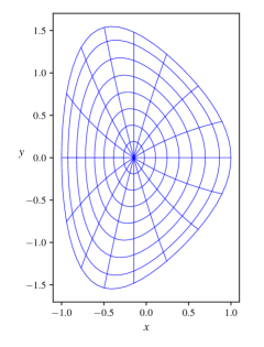
Figure 1: Disk-like domains defined by the mappings (2) (left) and (3) (right). Lines originating from the pole are isolines at constant $\theta$ and lines concentric around the pole are isolines at constant $s$.

In all the numerical tests considered in this work, mapping (2) is set up with the parameters

$$(x_{0},y_{0})=(0,0)\,,\quad\kappa=0.3\,,\quad\Delta=0.2\,,$$ (4)

and mapping (3) is set up with the parameters

$$y_{0}=0\,,\quad\varepsilon=0.3\,,\quad e=1.4\,,$$ (5)

which yield $x_{0}\approx-0.15$. Figure 1 shows the physical domains obtained with these mappings.

3 Discrete spline mappings

In practical applications it may not be possible to have an analytical description of the mapping that represents the physical domain of interest, as in the examples discussed above. Moreover, we are going to solve the elliptic equation in (1) with a finite element method based on $B$-splines. Our numerical method is therefore based on a machinery inherently defined at the discrete level. Hence, we need to have a discrete counterpart of the analytical singular mapped disk-like domains discussed in the previous section.

We start by defining a 2D tensor-product spline basis of clamped $B$-splines of degree $p_{1}$ in $s\in[0,1]$ and ${2\pi\text{-periodic}}$ $B$-splines of degree $p_{2}$ in $\theta\in[0,2\pi)$: $\{\widehat{B}_{i_{1}i_{2}}(s,\theta):=\widehat{B}_{i_{1}}^{s}(s)\widehat{B}_{i_{2}}^{\theta}(\theta)\,\}_{i_{1},i_{2}=1}^{n_{1},n_{2}}$. The domain along each direction is decomposed into 1D intervals, also referred to as cells, whose limit points are named break points. More precisely, the domain $[0,1]$ along $s$ is decomposed into ${n_{1}^{c}:=n_{1}-p_{1}}$ cells with ${n_{1}^{b}:=n_{1}^{c}+1}$ break points, denoted by $\{\widebar{s}_{i_{1}}\}_{i_{1}=1}^{n_{1}^{b}}$, and the domain $[0,2\pi)$ along $\theta$ is decomposed into ${n_{2}^{c}:=n_{2}}$ cells with ${n_{2}^{b}:=n_{2}^{c}+1}$ break points, denoted by $\{\widebar{\theta}_{i_{2}}\}_{i_{2}=1}^{n_{2}^{b}}$. From the break points, we define a knot sequence $\{t^{s}_{i_{1}}\}_{i_{1}=1-p_{1}}^{n^{b}_{1}+p_{1}}$ of $n_{1}^{b}+2p_{1}$ open knots along $s$ and a knot sequence $\{t^{\theta}_{i_{2}}\}_{i_{2}=1-p_{2}}^{n^{b}_{2}+p_{2}}$ of $n_{2}^{b}+2p_{2}$ periodic knots along $\theta$:

$$t^{s}_{i_{1}}:=\begin{dcases}\widebar{s}_{1}&i_{1}=1-p_{1},\dots,0\\ \widebar{s}_{i_{1}}&i_{1}=1,\dots,n^{b}_{1}\\ \widebar{s}_{n^{b}_{1}}&i_{1}=n^{b}_{1}+1,\dots,n^{b}_{1}+p_{1}\end{dcases}\quad t^{\theta}_{i_{2}}:=\begin{dcases}\widebar{\theta}_{n^{b}_{2}+i_{2}}-2\pi&i_{2}=1-p_{2},\dots,0\\ \widebar{\theta}_{i_{2}}&i_{2}=1,\dots,n^{b}_{2}\\ \widebar{\theta}_{i_{2}-n^{b}_{2}}+2\pi&i_{2}=n^{b}_{2}+1,\dots,n^{b}_{2}+p_{2}\end{dcases}$$

Due to the open knot sequence, the basis functions $\widehat{B}_{i_{1}}^{s}(s)$ satisfy the following properties:

$$\widehat{B}_{1}^{s} (0)=1\,,\quad \widehat{B}_{i_{1}}^{s}(0)=0\quad\text{for}\quad i_{1}=2,\dots,n_{1}\,,$$

$$\widehat{B}_{n_{1}}^{s} (1)=1\,,\quad \widehat{B}_{i_{1}}^{s}(1)=0\quad\text{for}\quad i_{1}=1,\dots,n_{1}-1\,.$$

Moreover, their derivatives satisfy the following property:

$$(\widehat{B}_{1}^{s})^{\prime}(0)=-(\widehat{B}_{2}^{s})^{\prime}(0)\neq 0\,,\quad(\widehat{B}_{i_{1}}^{s})^{\prime}(0)=0\quad\text{for}\quad i_{1}=3,\dots,n_{1}\,.$$

Based on this spline basis, we define a discrete representation of our analytical singular mapped disk-like domains as

$$x(s,\theta):=\sum_{i_{1}=1}^{n_{1}}\sum_{i_{2}=1}^{n_{2}}c_{i_{1}i_{2}}^{x}\widehat{B}_{i_{1}}^{s}(s)\widehat{B}_{i_{2}}^{\theta}(\theta)=x_{0}\,\widehat{B}_{1}^{s}(s)+\sum_{i_{1}=2}^{n_{1}}\sum_{i_{2}=1}^{n_{2}}c_{i_{1}i_{2}}^{x}\widehat{B}_{i_{1}}^{s}(s)\widehat{B}_{i_{2}}^{\theta}(\theta)\,,$$ (6)

$$y(s,\theta):=\sum_{i_{1}=1}^{n_{1}}\sum_{i_{2}=1}^{n_{2}}c_{i_{1}i_{2}}^{y}\widehat{B}_{i_{1}}^{s}(s)\widehat{B}_{i_{2}}^{\theta}(\theta)=y_{0}\,\widehat{B}_{1}^{s}(s)+\sum_{i_{1}=2}^{n_{1}}\sum_{i_{2}=1}^{n_{2}}c_{i_{1}i_{2}}^{y}\widehat{B}_{i_{1}}^{s}(s)\widehat{B}_{i_{2}}^{\theta}(\theta)\,.$$

The control points $(c_{i_{1}i_{2}}^{x},c_{i_{1}i_{2}}^{y})$ are obtained by interpolating the corresponding analytical mapping on the so-called Greville points [30, 31], defined as

$$s_{i_{1}} :=\frac{1}{p_{1}}\sum_{j_{1}=i_{1}+1-p_{1}}^{i_{1}}t^{s}_{j_{1}}\,,\quad i_{1}=1,\dots,n_{1}\,,$$ (7)

$$\theta_{i_{2}} :=\frac{1}{p_{2}}\sum_{j_{2}=i_{2}+1-p_{2}}^{i_{2}}t^{\theta}_{j_{2}}\,,\quad i_{2}=1,\dots,n_{2}\,.$$

Such points are averages of the knots generally lying near the values corresponding to the maximum of the basis functions. In the case of a periodic domain the Greville averages reduce to either the break points themselves or the mid-points of each cell, depending on whether the degree of the $B$-splines is odd or even, respectively. For more general practical applications, for example in the context of magnetized fusion plasmas, the control points $(c_{i_{1}i_{2}}^{x},c_{i_{1}i_{2}}^{y})$ could be given as an input from any code capable of constructing a mesh conformal to the flux surfaces of a given equilibrium magnetic field, such as, for example, the software Tokamesh [32]. Finally, we note that all the control points at $i_{1}=1$ are equal to the pole, $(c_{1i_{2}}^{x},c_{1i_{2}}^{y})=(x_{0},y_{0})$, which is another way of saying that the edge $s=0$ of the logical domain collapses to the pole of the physical domain.

In order to compute integrals on the logical domain, $1+p_{1}$ Gauss-Legendre quadrature points and weights are introduced in each cell of the domain $[0,1]$ along $s$ and $1+p_{2}$ Gauss-Legendre quadrature points and weights are introduced in each cell of the domain $[0,2\pi)$ along $\theta$.

4 Semi-Lagrangian advection solver

We now consider the hyperbolic advection equation in the guiding-center model (1):

$$\dfrac{\partial\rho}{\partial t}-E^{y}\dfrac{\partial\rho}{\partial x}+E^{x}\dfrac{\partial\rho}{\partial y}=0\,.$$ (8)

We are interested in solving (8) with the backward semi-Lagrangian method, which we review briefly in the following. We first note that (8) can be also written as

$$\frac{\textrm{d}}{\textrm{d}t}\,\rho(t,\boldsymbol{x}(t))=0\,,$$ (9)

with

$$\frac{\textrm{d}\boldsymbol{x}}{\textrm{d}t}=\boldsymbol{A}(t,\boldsymbol{x})\,,$$ (10)

where we introduced the advection field $\boldsymbol{A}:=(-E^{y},E^{x})^{T}$. The characteristics of (9) (and, equivalently, (8)) are the solutions of the dynamical system (10) with given initial conditions. The information contained in (9) is that its solution $\rho$ is conserved along the characteristics (10). When we solve (9) numerically, we are interested in knowing the value of $\rho$ at a given time $t$ and a given mesh point $\boldsymbol{x}_{ij}$ (assuming to have a mesh in the Cartesian coordinates $\boldsymbol{x}$), and the information at our disposal is the set of values of $\rho$ at the previous time $t-\Delta t$ at each mesh point. We then integrate the characteristics (10) backward in time to find the origin $\boldsymbol{x}_{ij}^{*}$ at time $t-\Delta t$ of the characteristic passing through $\boldsymbol{x}_{ij}$ at time $t$, and set $\rho(t,\boldsymbol{x}_{ij})=\rho(t-\Delta t,\boldsymbol{x}_{ij}^{*})$. Typically, the point $\boldsymbol{x}_{ij}^{*}$ does not coincide with a mesh point and the value $\rho(t-\Delta t,\boldsymbol{x}_{ij}^{*})$, which is not immediately available, is obtained by interpolating the values of $\rho$ at time $t-\Delta t$ and at mesh points in some neighborhood of $\boldsymbol{x}_{ij}^{*}$.

We now discuss the optimal choice of coordinates for the integration of the characteristics (10). In the following we denote $\textrm{d}\boldsymbol{x}/\textrm{d}t$ as $\accentset{\mbox{\Large\hskip 1.54999pt.}}{\boldsymbol{x}}$ and recall that the advection field available at the discrete level is the advection field $\widehat{\boldsymbol{A}}$ defined on the logical domain. It is natural to think of integrating the characteristic equations in either Cartesian or logical coordinates. However, both choices present some drawbacks. The characteristic equations in Cartesian coordinates $\boldsymbol{x}$ read

$$\accentset{\mbox{\Large\hskip 1.54999pt.}}{\boldsymbol{x}}=\widehat{\boldsymbol{A}}(t,\boldsymbol{F}^{-1}(\boldsymbol{x}))\,.$$ (11)

These equations are well-defined everywhere in the domain, but they become computationally expensive if the mapping $\boldsymbol{F}$ is not easy to invert. On the other hand, the characteristic equations in logical coordinates $\boldsymbol{\eta}$ read

$$\accentset{\mbox{\Large\hskip 1.54999pt.}}{\boldsymbol{\eta}}=J_{\boldsymbol{F}}^{-1}\widehat{\boldsymbol{A}}(t,\boldsymbol{\eta})\,.$$ (12)

These equations are not defined at the pole $s=0$, because $J_{\boldsymbol{F}}^{-1}$ is singular there. We then suggest to introduce the new coordinates $\boldsymbol{X}:=(X,Y)$ defined by the polar transformation

$$X(s,\theta):=s\cos\theta\,,$$ (13)

$$Y(s,\theta):=s\sin\theta\,,$$

which we name pseudo-Cartesian coordinates. We denote by $\boldsymbol{G}:\widehat{\Omega}\to\mathbb{R}^{2}$ the new mapping defined by $\boldsymbol{G}(\boldsymbol{\eta}):=\boldsymbol{X}$, and by $J_{\boldsymbol{G}}$ its Jacobian, given by

$$J_{\boldsymbol{G}}(s,\theta)=\begin{bmatrix}\cos\theta&-s\sin\theta\\ \sin\theta&\phantom{-}s\cos\theta\end{bmatrix}\,.$$

The pseudo-Cartesian coordinates for the domains defined by the mappings (2) and (3) are shown in Figure 2. In the simplest case of a circular mapping, they reduce to standard Cartesian coordinates. The characteristic equations in pseudo-Cartesian coordinates $\boldsymbol{X}$ read

$$\accentset{\mbox{\Large\hskip 1.54999pt.}}{\boldsymbol{X}}=(J_{\boldsymbol{F}}J_{\boldsymbol{G}}^{-1})^{-1}\widehat{\boldsymbol{A}}(t,\boldsymbol{G}^{-1}(\boldsymbol{X}))\,,$$ (14)

where $J_{\boldsymbol{F}}J_{\boldsymbol{G}}^{-1}$ represents the Jacobian of the composite mapping $\boldsymbol{F}\circ\boldsymbol{G}^{-1}$ defined by ${\boldsymbol{F}\circ\boldsymbol{G}^{-1}(\boldsymbol{X})=\boldsymbol{x}}$. For a circular mapping, $\boldsymbol{F}\circ\boldsymbol{G}^{-1}$ reduces to the identity and (14) reduces to (11), which works well because $\boldsymbol{F}^{-1}$ (inverse polar transformation) is easy to compute. For more complex non-circular mappings, (14) is more convenient than (11) because the mapping $\boldsymbol{G}$ is easier to invert than the original mapping $\boldsymbol{F}$. More precisely, the inverse mapping $\boldsymbol{G}^{-1}$ is analytical and reads

$$s(X,Y) =\sqrt{X^{2}+Y^{2}}\,,$$ (15)

$$\theta(X,Y) =\text{atan}2(Y,X)\,,$$

where $\text{atan}2(Y,X)$ returns the principal value of the argument function applied to the complex number $X+iY$ in the range $(-\pi,\pi]$ (which then must be shifted appropriately to the domain $[0,2\pi)$). Moreover, the inverse Jacobian matrix $(J_{\boldsymbol{F}}J_{\boldsymbol{G}}^{-1})^{-1}$ in (14) turns out to be well-behaved everywhere in the physical domain, including the pole.

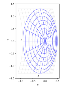
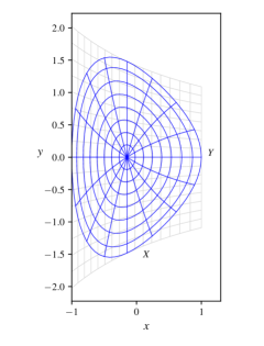
Figure 2: Pseudo-Cartesian coordinates: the light-gray grids represent the grids in the pseudo-Cartesian coordinates $(X,Y)$ for disk-like domains defined by the mappings (2) (left) and (3) (right).

More precisely, the singularity of the inverse Jacobian matrix

$$J_{\boldsymbol{G}}^{-1}(s,\theta)=\begin{bmatrix}\cos\theta&\sin\theta\\[5.69054pt] -\dfrac{1}{s}\sin\theta&\dfrac{1}{s}\cos\theta\end{bmatrix}\,,$$

in the limit $s\to 0^{+}$, is canceled by the matrix elements of $J_{\boldsymbol{F}}$. The product $J_{\boldsymbol{F}}J_{\boldsymbol{G}}^{-1}$ in general reads

$$J_{\boldsymbol{F}}J_{\boldsymbol{G}}^{-1}(s,\theta)=\begin{bmatrix}\dfrac{\partial x}{\partial s}\cos\theta-\dfrac{1}{s}\dfrac{\partial x}{\partial\theta}\sin\theta&\dfrac{\partial x}{\partial s}\sin\theta+\dfrac{1}{s}\dfrac{\partial x}{\partial\theta}\cos\theta\\ \dfrac{\partial y}{\partial s}\cos\theta-\dfrac{1}{s}\dfrac{\partial y}{\partial\theta}\sin\theta&\dfrac{\partial y}{\partial s}\sin\theta+\dfrac{1}{s}\dfrac{\partial y}{\partial\theta}\cos\theta\end{bmatrix}\,.$$ (16)

From an analytical point of view, (16) holds for all values of $s$ except at the pole $s=0$. However, the products $\dfrac{1}{s}\dfrac{\partial x}{\partial\theta}$ and $\dfrac{1}{s}\dfrac{\partial y}{\partial\theta}$ are finite and well-defined in the limit $s\to 0^{+}$. From a numerical point of view, (16) holds for all values of $s$ sufficiently far from the pole, as far as the factor $1/s$ does not become too large. Therefore, we assume that (16) holds for $s\geq\epsilon$, for a given small $\epsilon$. More precisely, the derivatives $\partial x/\partial\theta$ and $\partial y/\partial\theta$ vanish for $s=0$. Hence, expanding in $s$ around $s=0$, we have

$$\frac{\partial x}{\partial\theta}(s,\theta)=\frac{\partial x}{\partial\theta}(0,\theta)+s\,\frac{\partial^{2}x}{\partial s\,\partial\theta}(0,\theta)+O(s^{2})=s\,\frac{\partial^{2}x}{\partial s\,\partial\theta}(0,\theta)+O(s^{2})\,,$$

$$\frac{\partial y}{\partial\theta}(s,\theta)=\frac{\partial y}{\partial\theta}(0,\theta)+s\,\frac{\partial^{2}y}{\partial s\,\partial\theta}(0,\theta)+O(s^{2})=s\,\frac{\partial^{2}y}{\partial s\,\partial\theta}(0,\theta)+O(s^{2})\,,$$

which yields

$$\lim_{s\to 0^{+}}\frac{1}{s}\frac{\partial x}{\partial\theta}(s,\theta)=\frac{\partial^{2}x}{\partial s\,\partial\theta}(0,\theta)\,,$$

$$\lim_{s\to 0^{+}}\frac{1}{s}\frac{\partial y}{\partial\theta}(s,\theta)=\frac{\partial^{2}y}{\partial s\,\partial\theta}(0,\theta)\,.$$

Therefore, the product $J_{\boldsymbol{F}}J_{\boldsymbol{G}}^{-1}$ at the pole $s=0$ reads

$$J_{\boldsymbol{F}}J_{\boldsymbol{G}}^{-1}(0,\theta)=\begin{bmatrix}\dfrac{\partial x}{\partial s}(0,\theta)\cos\theta-\dfrac{\partial^{2}x}{\partial s\,\partial\theta}(0,\theta)\sin\theta&\dfrac{\partial x}{\partial s}(0,\theta)\sin\theta+\dfrac{\partial^{2}x}{\partial s\,\partial\theta}(0,\theta)\cos\theta\\ \dfrac{\partial y}{\partial s}(0,\theta)\cos\theta-\dfrac{\partial^{2}y}{\partial s\,\partial\theta}(0,\theta)\sin\theta&\dfrac{\partial y}{\partial s}(0,\theta)\sin\theta+\dfrac{\partial^{2}y}{\partial s\,\partial\theta}(0,\theta)\cos\theta\end{bmatrix}\,.$$ (17)

For example, in the case of mapping (2) we get

$$(J_{\boldsymbol{F}}J_{\boldsymbol{G}}^{-1})^{-1}(0,\theta)=\begin{bmatrix}\dfrac{1}{1-\kappa}&0\\[5.69054pt] 0&\dfrac{1}{1+\kappa}\end{bmatrix}\,,$$ (18)

and, similarly, in the case of mapping (3) we get

$$(J_{\boldsymbol{F}}J_{\boldsymbol{G}}^{-1})^{-1}(0,\theta)=\begin{bmatrix}-\sqrt{1+\varepsilon^{2}}&0\\[5.69054pt] 0&\dfrac{2-\sqrt{1+\varepsilon^{2}}}{e\,\xi}\end{bmatrix}\,.$$ (19)

In order to connect (16) and (17) in a smooth way, for $0<s<\epsilon$ we interpolate linearly the value at the pole $s=0$ and the value at $s=\epsilon$, obtaining

$$(J_{\boldsymbol{F}}J_{\boldsymbol{G}}^{-1})^{-1}(s,\theta)=\bigg{(}1-\frac{s}{\epsilon}\bigg{)}(J_{\boldsymbol{F}}J_{\boldsymbol{G}}^{-1})^{-1}(0,\theta)+\frac{s}{\epsilon}(J_{\boldsymbol{F}}J_{\boldsymbol{G}}^{-1})^{-1}(\epsilon,\theta)\,.$$

We remark that the result obtained in (17) needs to be single-valued, and hence should not depend on the angle-like variable $\theta$. This is true if we consider analytical mappings such as (2) and (3), as demonstrated by (18) and (19), respectively. If we consider, instead, a discrete representation of the aforementioned mappings, defined, for example, in terms of splines, we observe a residual dependence of (17) on $\theta$. It is possible to measure the discrepancy between the matrix elements of $(J_{\boldsymbol{F}}J_{\boldsymbol{G}}^{-1})^{-1}(0,\theta)$, computed by inverting (17) (with the derivatives evaluated from the discrete spline mapping (6)), and the corresponding analytical $\theta$-independent matrix elements. As a measure of the error, we consider the maximum among all matrix elements and all values of $\theta$ for a given interpolation grid. The results in Table 1 show that such errors become asymptotically small as the computational mesh is refined (that is, as the number of interpolation points is increased). Such errors do not constitute a problem if they turn out to be smaller than the overall numerical accuracy of our scheme. However, we suggest to guarantee that (17) is truly single-valued by taking an average of (17) over all values of $\theta$ in the interpolation grid. This may become particularly useful if implicit integration schemes are used, when the magnitude of the aforementioned errors may become comparable to the tolerances chosen for the implicit methods of choice.

	Circular mapping		Mapping (2)		Mapping (3)
$n_{1}\times n_{2}$	Error	Order	Error	Order	Error	Order
$16\times 32$	$8.30\times 10^{-6}$		$1.19\times 10^{-5}$		$8.66\times 10^{-6}$
$32\times 64$	$5.17\times 10^{-7}$	$4.01$	$7.38\times 10^{-7}$	$4.01$	$5.39\times 10^{-7}$	$4.01$
$64\times 128$	$3.23\times 10^{-8}$	$4.00$	$4.61\times 10^{-8}$	$4.00$	$3.37\times 10^{-8}$	$4.00$
$128\times 256$	$2.02\times 10^{-9}$	$4.00$	$2.88\times 10^{-9}$	$4.00$	$2.94\times 10^{-9}$	$3.52$
$256\times 512$	$1.26\times 10^{-10}$	$4.00$	$1.80\times 10^{-10}$	$4.00$	$3.69\times 10^{-10}$	$3.00$

Table 1: Convergence of the product $(J_{\boldsymbol{F}}J_{\boldsymbol{G}}^{-1})^{-1}$ to the corresponding $\theta$-independent analytical values for a circular mapping and for the mappings (2) and (3).

We also remark that the parameter $\epsilon$ can be chosen arbitrarily small, as far as it avoids underflows and overflows in floating point arithmetic. For all the numerical tests discussed in this work we set $\epsilon=10^{-12}$. We note that the origin of a given characteristic may be located arbitrarily close to the pole (with the pole itself being indeed the first point of our computational mesh in the radial-like direction $s$). Therefore, a numerical strategy for the computation of the product $(J_{\boldsymbol{F}}J_{\boldsymbol{G}}^{-1})^{-1}$ at the pole and in the region close to it, where the factor $1/s$ appearing in (16) is numerically too large, cannot be avoided.

4.1 Numerical tests

We test the advection solver for the stationary rotating advection field

$$\boldsymbol{A}(x,y):=\omega\begin{pmatrix}y_{c}-y\\ x-x_{c}\end{pmatrix}\,,$$ (20)

with $\omega=2\pi$ and $(x_{c},y_{c})=(0.25,0)$. The numerical test is performed on mapping (3) with the parameters in (5). The flow field corresponding to the advection field (20) can be computed analytically and reads

$$x(t+\Delta t)=x_{c}+\left(x(t)-x_{c}\right)\cos(\omega\Delta t)-\left(y(t)-y_{c}\right)\sin(\omega\Delta t)\,,$$ (21)

$$y(t+\Delta t)=y_{c}+\left(x(t)-x_{c}\right)\sin(\omega\Delta t)+\left(y(t)-y_{c}\right)\cos(\omega\Delta t)\,,$$

where $\Delta t$ denotes the time step. Therefore, the numerical solution can be compared to the exact one obtained from the analytical flow field by the method of characteristics, $\rho_{\text{ex}}(t,x(t),y(t))=\rho(0,x(0),y(0))$, where the initial position $(x(0),y(0))$ is obtained from (21) with $\Delta t=-t$. The initial condition is set to a superposition of cosine bells with elliptical cross sections:

$$\rho(0,x,y):=\frac{1}{2}\bigg{[}\mathcal{G}\big{(}r_{1}(x,y)\big{)}+\mathcal{G}(r_{2}(x,y)\big{)}\bigg{]}\,,$$

with $\mathcal{G}(r)$ defined as

$$\mathcal{G}(r):=\begin{dcases}\cos\bigg{(}\frac{\pi r}{2a}\bigg{)}^{4}&r<a\,,\\ 0&\text{elsewhere}\,,\end{dcases}$$

with $a=0.3$, and $r_{1}(x,y)$ and $r_{2}(x,y)$ defined as

$$r_{1}(x,y):=\sqrt{(x-x_{0})^{2}+8(y-y_{0})^{2}}\,,\quad r_{2}(x,y):=\sqrt{8(x-x_{0})^{2}+(y-y_{0})^{2}}\,.$$

This test case is inspired by one presented in [33, section 5.2]: the non-Gaussian initial condition allows us to possibly detect any deformation of the initial density perturbation while rotating under the action of the advection field (20).

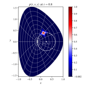
Figure 3: Numerical test of the advection solver: contour plot of the density $\rho$ at a given time. The dashed circle represents the trajectory that the initial density perturbation is expected to follow under the action of the rotating advection field (20).

Denoting by ${\Delta\rho:=\rho-\rho_{\text{ex}}}$ the numerical error, that is, the difference between the numerical solution and the exact one, measures of the error of our numerical scheme are obtained by taking the $L^{\infty}$-norm in time of the spatial $L^{2}$-norm of $\Delta\rho$,

$$\max_{t}||\Delta\rho||_{L^{2}}:=\max_{t}\left(\sqrt{\int_{\Omega}\textrm{d}x\,\textrm{d}y\,\left[\Delta\rho(t,x,y)\right]^{2}}\,\right)=\max_{t}\left(\sqrt{\int_{\widehat{\Omega}}\textrm{d}s\,\textrm{d}\theta\,|\det J_{\boldsymbol{F}}(s,\theta)|\,\left[\Delta\widehat{\rho}(t,s,\theta)\right]^{2}}\,\right)\,,$$

computed using the Gauss-Legendre quadrature points and weights mentioned in section 3, and the $L^{\infty}$-norm in time of the spatial $L^{\infty}$-norm of $\Delta\rho$,

$$\max_{t}||\Delta\rho||_{L^{\infty}}:=\max_{t}\max_{(x,y)\in\Omega}\,\left|\Delta\rho(t,x,y)\right|=\max_{t}\max_{(s,\theta)\in\widehat{\Omega}}\,\left|\Delta\widehat{\rho}(t,s,\theta)\right|\,,$$

computed on the Greville points (7). We remark that the pole is included when we estimate the spatial ${L^{\infty}\text{-norm}}$. Table 2 shows the convergence of our numerical scheme while decreasing the time step $\Delta t$ and correspondingly refining the spatial mesh by increasing the number of points $n_{1}$ in the direction $s$ and the number of points $n_{2}$ in the direction $\theta$ (in order to keep the CFL number constant), using cubic splines and an explicit third-order Runge-Kutta method for the integration of the characteristics. We note that there are no effects of order reduction due to the singularity at the pole. Standard tensor-product spline interpolation turns out to work well in the presence of analytical advection fields, provided our choice of coordinates for the time integration of the characteristics. The time integration algorithm is as follows. Starting from a mesh point $\boldsymbol{\eta}_{ij}:=(s_{i},\theta_{j})$ with pseudo-Cartesian coordinates $\boldsymbol{X}_{ij}:=\boldsymbol{G}(\boldsymbol{\eta}_{ij})$, we compute the first-stage, second-stage and third-stage derivatives and solutions

$$1.\quad\accentset{\mbox{\Large\hskip 1.54999pt.}}{\boldsymbol{X}}_{ij}^{(1)}:=(J_{\boldsymbol{F}}J_{\boldsymbol{G}}^{-1})^{-1}(\boldsymbol{\eta}_{ij})\,\widehat{\boldsymbol{A}}(\boldsymbol{\eta}_{ij}) \,,\quad \boldsymbol{X}_{ij}^{(1)}:=\boldsymbol{X}_{ij}-\frac{\Delta t}{2}\accentset{\mbox{\Large\hskip 1.54999pt.}}{\boldsymbol{X}}_{ij}^{(1)} \,,\quad \boldsymbol{\eta}_{ij}^{(1)}:=\boldsymbol{G}^{-1}(\boldsymbol{X}_{ij}^{(1)})\,;$$

$$2.\quad\accentset{\mbox{\Large\hskip 1.54999pt.}}{\boldsymbol{X}}_{ij}^{(2)}:=(J_{\boldsymbol{F}}J_{\boldsymbol{G}}^{-1})^{-1}(\boldsymbol{\eta}_{ij}^{(1)})\,\widehat{\boldsymbol{A}}(\boldsymbol{\eta}_{ij}^{(1)}) \,,\quad \boldsymbol{X}_{ij}^{(2)}:=\boldsymbol{X}_{ij}-\Delta t\left[2\accentset{\mbox{\Large\hskip 1.54999pt.}}{\boldsymbol{X}}_{ij}^{(2)}-\accentset{\mbox{\Large\hskip 1.54999pt.}}{\boldsymbol{X}}_{ij}^{(1)}\right] \,,\quad \boldsymbol{\eta}_{ij}^{(2)}:=\boldsymbol{G}^{-1}(\boldsymbol{X}_{ij}^{(2)})\,;$$

$$3.\quad\accentset{\mbox{\Large\hskip 1.54999pt.}}{\boldsymbol{X}}_{ij}^{(3)}:=(J_{\boldsymbol{F}}J_{\boldsymbol{G}}^{-1})^{-1}(\boldsymbol{\eta}_{ij}^{(2)})\,\widehat{\boldsymbol{A}}(\boldsymbol{\eta}_{ij}^{(2)}) \,,\quad \boldsymbol{X}_{ij}^{(3)}:=\boldsymbol{X}_{ij}-\frac{\Delta t}{6}\left[\accentset{\mbox{\Large\hskip 1.54999pt.}}{\boldsymbol{X}}_{ij}^{(1)}+4\accentset{\mbox{\Large\hskip 1.54999pt.}}{\boldsymbol{X}}_{ij}^{(2)}+\accentset{\mbox{\Large\hskip 1.54999pt.}}{\boldsymbol{X}}_{ij}^{(3)}\right] \,,\quad \boldsymbol{\eta}_{ij}^{(3)}:=\boldsymbol{G}^{-1}(\boldsymbol{X}_{ij}^{(3)})\,.$$

The logical coordinates $\boldsymbol{\eta}_{ij}^{(3)}$ obtained represent the origin of the characteristic at time $t-\Delta t$ passing through the point $\boldsymbol{\eta}_{ij}$ at time $t$.

$\Delta t$	$n_{1}\times n_{2}$	$\max_{t}||\Delta\rho||_{L^{2}}$	Order	$\max_{t}||\Delta\rho||_{L^{\infty}}$	Order
$0.1$	$64\times 128$	$3.25\times 10^{-2}$		$3.53\times 10^{-1}$
$0.1/2$	$128\times 256$	$4.10\times 10^{-3}$	2.99	$4.34\times 10^{-2}$	$3.02$
$0.1/4$	$256\times 512$	$5.11\times 10^{-4}$	3.00	$5.09\times 10^{-3}$	$3.09$
$0.1/8$	$512\times 1024$	$6.39\times 10^{-5}$	3.00	$6.13\times 10^{-4}$	$3.05$
$0.1/16$	$1024\times 2048$	$7.98\times 10^{-6}$	3.00	$7.52\times 10^{-5}$	$3.03$

Table 2: Third-order convergence of the advection solver using cubic splines and an explicit third-order Runge-Kutta method for the integration of the characteristics.

5 Finite element elliptic solver

We now focus on the elliptic Poisson equation in the guiding-center model (1):

$$-\boldsymbol{\nabla}\cdot\boldsymbol{\nabla}\phi=\rho\,.$$ (22)

We want to solve this equation with a finite element method based on $B$-splines. Following an isogeometric analysis approach, we use the same spline basis used to construct the discrete spline mappings as a basis for our finite element method. The aim is to obtain a potential $\phi$ which is $\mathcal{C}^{1}$ smooth everywhere in the physical domain, including the pole, so that the corresponding advection fields for the transport of $\rho$ are continuous. This is achieved by imposing appropriate $\mathcal{C}^{1}$ smoothness constraints on the spline basis while solving the linear system obtained from the weak form of (22). A systematic approach to define a set of globally $\mathcal{C}^{1}$ smooth spline basis functions on singular mapped disk-like domains was developed in [27] and we now recall its basic ideas ([27] actually suggests a more general procedure valid also for higher-order smoothness, consistent with the spline degree).

5.1 $\mathcal{C}^{1}$ smooth polar splines

The idea is to satisfy the $\mathcal{C}^{1}$ smoothness requirements by imposing appropriate constraints on the $2n_{2}$ degrees of freedom corresponding to $i_{1}=1,2$ for all $i_{2}$. More precisely, the $2n_{2}$ basis functions corresponding to these degrees of freedom are replaced by only three new basis functions, defined as linear combinations of the existing ones. In order to guarantee the properties of partition of unity and positivity, [27] suggests to use barycentric coordinates to construct these linear combinations. Taking an equilateral triangle enclosing the pole and the first row of control points $(c_{2\,i_{2}}^{x},c_{2\,i_{2}}^{y})$, with vertices

$$V_{1}:=(x_{0}+\tau,y_{0})\,,\quad V_{2}:=\left(x_{0}-\frac{\tau}{2},y_{0}+\frac{\sqrt{3}}{2}\tau\right)\,,\quad V_{3}:=\left(x_{0}-\frac{\tau}{2},y_{0}-\frac{\sqrt{3}}{2}\tau\right)\,,$$

where $(x_{0},y_{0})$ denotes the Cartesian coordinates of the pole and $\tau$ is defined as

$$\tau:=\max\left[\max_{i_{2}}\left(-2(c_{2\,i_{2}}^{x}-x_{0})\right),\max_{i_{2}}\left((c_{2\,i_{2}}^{x}-x_{0})-\sqrt{3}(c_{2\,i_{2}}^{y}-y_{0})\right),\max_{i_{2}}\left((c_{2\,i_{2}}^{x}-x_{0})+\sqrt{3}(c_{2\,i_{2}}^{y}-y_{0})\right)\right]\,,$$

we denote by $(\lambda_{1},\lambda_{2},\lambda_{3})$ the barycentric coordinates of any point with respect to the vertices of this triangle:

$$\lambda_{1}(x,y):=\frac{1}{3}+\frac{2}{3}\frac{1}{\tau}(x-x_{0})\,,$$

$$\lambda_{2}(x,y):=\frac{1}{3}-\frac{1}{3}\frac{1}{\tau}(x-x_{0})+\frac{\sqrt{3}}{3}\frac{1}{\tau}(y-y_{0})\,,$$

$$\lambda_{3}(x,y):=\frac{1}{3}-\frac{1}{3}\frac{1}{\tau}(x-x_{0})-\frac{\sqrt{3}}{3}\frac{1}{\tau}(y-y_{0})\,.$$

Then, the three new basis functions are denoted by $\widehat{\mathcal{B}}_{l}$, for $l=1,2,3$, and defined as

$$\widehat{\mathcal{B}}_{l}(s,\theta):=\sum_{i_{1}=1}^{2}\sum_{i_{2}=1}^{n_{2}}\lambda_{l}(c_{i_{1}i_{2}}^{x},c_{i_{1}i_{2}}^{y})\widehat{B}_{i_{1}}^{s}(s)\widehat{B}_{i_{2}}^{\theta}(\theta)\,.$$

It is easy to show that these basis functions are positive, $\widehat{\mathcal{B}}_{l}(s,\theta)\geq 0$ $\forall(s,\theta)$ and $\forall l$, and that they satisfy the partition of unity property, namely

$$\sum_{l=1}^{3}\widehat{\mathcal{B}}_{l}(s,\theta)+\sum_{i_{1}=3}^{n_{1}}\sum_{i_{2}=1}^{n_{2}}\widehat{B}_{i_{1}}^{s}(s)\widehat{B}_{i_{2}}^{\theta}(\theta)=1\quad\forall(s,\theta)\,.$$ (23)

Moreover, the new basis functions $\mathcal{B}_{l}$, related to $\widehat{\mathcal{B}}_{l}$ via $\widehat{\mathcal{B}}_{l}=\mathcal{B}_{l}\circ\boldsymbol{F}$, are $\mathcal{C}^{1}$ smooth everywhere in the physical domain.

5.2 Finite element solver

We now consider a more general version of Poisson’s equation (22) which includes a finite set of $n_{c}$ point charges, denoted with the label $c$, of charges $q_{c}$ and positions $(x_{c},y_{c})$. Denoting by $\rho_{\text{SL}}$ and $\rho_{\text{PIC}}$ the semi-Lagrangian density and the particle density, respectively, we rewrite (22) as

$$-\boldsymbol{\nabla}\cdot\boldsymbol{\nabla}\phi=\rho_{\text{SL}}+\rho_{\text{PIC}}\,,\quad\text{with}\quad\rho_{\text{PIC}}(x,y):=\sum_{c=1}^{n_{c}}q_{c}\,\delta(x-x_{c})\delta(y-y_{c})\,,$$ (24)

with homogeneous Dirichlet boundary conditions $\phi(x,y)=0$ on $\partial\Omega$ (omitting the time dependence of $\phi$). We impose these boundary conditions by removing the corresponding basis functions from both the test space and the trial space. More precisely, we choose as test and trial spaces the space defined by the tensor-product spline basis ${\{\widehat{B}_{i_{1}i_{2}}(s,\theta):=\widehat{B}_{i_{1}}^{s}(s)\widehat{B}_{i_{2}}^{\theta}(\theta)\,\}_{i_{1},i_{2}=1}^{n_{1}-1,n_{2}}}$, where we remove the last $n_{2}$ basis functions corresponding to $i_{1}=n_{1}$. Hence, the weak form of (24) reads

$$\int_{\Omega}\textrm{d}x\,\textrm{d}y\,\boldsymbol{\nabla}\phi\cdot\boldsymbol{\nabla}B_{i_{1}i_{2}}=\int_{\Omega}\textrm{d}x\,\textrm{d}y\,\rho_{\text{SL}}\,B_{i_{1}i_{2}}+\sum_{c=1}^{n_{c}}q_{c}B_{i_{1}i_{2}}(x_{c},y_{c})\,,\quad\forall i_{1},i_{2}\,.$$

We now expand $\phi$ on the trial space,

$$\phi=\sum_{j_{1}=1}^{n_{1}-1}\sum_{j_{2}=1}^{n_{2}}\phi_{j_{1}j_{2}}\,B_{j_{1}j_{2}}\,,$$

and $\rho_{\text{SL}}$ on the full tensor-product space (without removing the last $n_{2}$ basis functions, as the space where $\rho_{\text{SL}}$ is defined is completely independent from the test and trial spaces),

$$\rho_{\text{SL}}=\sum_{k_{1}=1}^{n_{1}}\sum_{k_{2}=1}^{n_{2}}\rho_{k_{1}k_{2}}\,B_{k_{1}k_{2}}\,.$$

To sum up, the following integer indices are being used:

$$i_{1}=1,\dots,n_{1}-1\qquad i_{2}=1,\dots,n_{2}\qquad\text{(test space)}$$

$$j_{1}=1,\dots,n_{1}-1\qquad j_{2}=1,\dots,n_{2}\qquad\text{(trial space)}$$

$$k_{1}=1,\dots,n_{1}\qquad k_{2}=1,\dots,n_{2}\qquad\text{(space of $\rho_{\text{SL}}$)}$$

Hence, we obtain

$$\sum_{j_{1}=1}^{n_{1}-1}\sum_{j_{2}=1}^{n_{2}}\phi_{j_{1}j_{2}}\int_{\Omega}\textrm{d}x\,\textrm{d}y\,\boldsymbol{\nabla}B_{j_{1}j_{2}}\cdot\boldsymbol{\nabla}B_{i_{1}i_{2}}=\sum_{k_{1}=1}^{n_{1}}\sum_{k_{2}=1}^{n_{2}}\rho_{k_{1}k_{2}}\int_{\Omega}\textrm{d}x\,\textrm{d}y\,B_{k_{1}k_{2}}\,B_{i_{1}i_{2}}+\sum_{c=1}^{n_{c}}q_{c}B_{i_{1}i_{2}}(x_{c},y_{c})\,,\quad\forall i_{1},i_{2}\,.$$

We now introduce the tensors

$$S_{i_{1}i_{2}j_{1}j_{2}} :=\int_{\Omega}\textrm{d}x\,\textrm{d}y\,\boldsymbol{\nabla}B_{j_{1}j_{2}}\cdot\boldsymbol{\nabla}B_{i_{1}i_{2}} =\int_{\widehat{\Omega}}\textrm{d}s\,\textrm{d}\theta\,|\det J_{\boldsymbol{F}}|\,\widehat{\boldsymbol{\nabla}}\widehat{B}_{j_{1}j_{2}}\cdot g^{-1}\cdot\widehat{\boldsymbol{\nabla}}\widehat{B}_{i_{1}i_{2}}\,,$$ (25)

$$M_{i_{1}i_{2}k_{1}k_{2}} :=\int_{\Omega}\textrm{d}x\,\textrm{d}y\,B_{k_{1}k_{2}}\,B_{i_{1}i_{2}} =\int_{\widehat{\Omega}}\textrm{d}s\,\textrm{d}\theta\,|\det J_{\boldsymbol{F}}|\,\widehat{B}_{k_{1}k_{2}}\,\widehat{B}_{i_{1}i_{2}}\,,$$

where $\widehat{\boldsymbol{\nabla}}$ denotes the gradient in the logical domain, defined as $\widehat{\boldsymbol{\nabla}}\widehat{f}:=\left(\dfrac{\partial\widehat{f}}{\partial s},\dfrac{\partial\widehat{f}}{\partial\theta}\right)^{T}$ for any function $\widehat{f}\in\mathcal{C}^{1}(\widehat{\Omega})$, and $g^{-1}$ denotes the inverse metric tensor of the logical coordinate system. Such integrals are computed using the Gauss-Legendre quadrature points and weights mentioned in section 3. We then obtain

$$\sum_{j_{1}=1}^{n_{1}-1}\sum_{j_{2}=1}^{n_{2}}S_{i_{1}i_{2}j_{1}j_{2}}\,\phi_{j_{1}j_{2}}=\sum_{k_{1}=1}^{n_{1}}\sum_{k_{2}=1}^{n_{2}}M_{i_{1}i_{2}k_{1}k_{2}}\,\rho_{k_{1}k_{2}}+\sum_{c=1}^{n_{c}}q_{c}\widehat{B}_{i_{1}i_{2}}(s_{c},\theta_{c})\,,\quad\forall i_{1},i_{2}\,.$$ (26)

Here, the basis functions $\widehat{B}_{i_{1}i_{2}}$ in the last term are evaluated at the positions $(s_{c},\theta_{c})=\boldsymbol{F}^{-1}(x_{c},y_{c})$ of the point charges in the logical domain. We remark that, when Poisson’s equation is coupled to the advection equation for $\rho$ in the guiding-center model, $\boldsymbol{F}^{-1}(x_{c},y_{c})$ needs only to be computed at the beginning of a simulation: later on, the particle equations of motion are integrated using the pseudo-Cartesian coordinates $(X_{c},Y_{c})$ and therefore ${(s_{c},\theta_{c})=\boldsymbol{G}^{-1}(X_{c},Y_{c})}$. Equation (26) can be written in matrix form as follows. Defining the new integer indices

$$i:=(i_{1}-1)n_{2}+i_{2} =1,\dots,(n_{1}-1)n_{2}\qquad$$ (test space)

$$j:=(j_{1}-1)n_{2}+j_{2} =1,\dots,(n_{1}-1)n_{2}\qquad$$ (trial space)

$$k:=(k_{1}-1)n_{2}+k_{2} =1,\dots,n_{1}n_{2}\qquad \rho_{\text{SL}}$$ (space of )

we can write (26) as

$$S\boldsymbol{\phi}=M\boldsymbol{\rho}_{\text{SL}}+\boldsymbol{\rho}_{\text{PIC}}\,,$$ (27)

where we introduced the matrices $S$ and $M$ with elements $(S)_{ij}:=S_{i_{1}i_{2}j_{1}j_{2}}$ and $(M)_{ik}:=M_{i_{1}i_{2}k_{1}k_{2}}$, and the vectors $\boldsymbol{\phi}$, $\boldsymbol{\rho}_{\text{SL}}$ and $\boldsymbol{\rho}_{\text{PIC}}$ with elements $(\boldsymbol{\phi})_{j}:=\phi_{j_{1}j_{2}}$, $(\boldsymbol{\rho}_{\text{SL}})_{k}:=\rho_{k_{1}k_{2}}$ and ${(\boldsymbol{\rho}_{\text{PIC}})_{i}:=\sum_{c=1}^{n_{c}}q_{c}\widehat{B}_{i_{1}i_{2}}(s_{c},\theta_{c})}$. The $\mathcal{C}^{1}$ smoothness constraint is imposed by applying to the tensor-product spline basis of the test and trial spaces the restriction operator (using a notation similar to [27, section 3.3])

$$E:=\begin{pmatrix}\widebar{E}&0\\ 0&I\end{pmatrix}\,,$$

where $\widebar{E}$ contains the barycentric coordinates of the pole and of the first row of control points. More precisely, $\widebar{E}$ is a $2n_{2}\times 3$ matrix with elements $\widebar{E}_{il}:=\lambda_{l}(c^{x}_{i_{1}i_{2}},c^{y}_{i_{1}i_{2}})$ and $I$ is the identity matrix of size $[(n_{1}-3)n_{2}]\times[(n_{1}-3)n_{2}]$. Hence, the restriction operator $E$ is a matrix of size $[(n_{1}-1)n_{2}]\times[3+(n_{1}-3)n_{2}]$. Therefore, (27) becomes

$$\widebar{S}\widebar{\boldsymbol{\phi}}=E^{T}(M\boldsymbol{\rho}_{\text{SL}}+\boldsymbol{\rho}_{\text{PIC}})\,,$$ (28)

where $\widebar{S}:=E^{T}SE$ and the solution vector $\widebar{\boldsymbol{\phi}}$ is of size $[3+(n_{1}-3)n_{2}]$. The matrix $\widebar{S}$ is symmetric and positive-definite, hence we can solve the linear system (28) with the conjugate gradient method [34, 35]. The resulting solution is then prolonged back to the trial space via $\boldsymbol{\phi}=E\widebar{\boldsymbol{\phi}}$.

5.3 Numerical tests

We test the Poisson solver with the method of manufactured solutions, looking for an exact solution of the form

$$\widehat{\phi}_{\text{ex}}(s,\theta):=(1-s^{2})\cos(2\pi\,x(s,\theta))\sin(2\pi\,y(s,\theta))\,,$$

on the physical domain defined by mapping (2). Denoting by ${\Delta\phi:=\phi-\phi_{\text{ex}}}$ the numerical error, that is the difference between the numerical solution and the exact one, measures of the error are obtained by computing the spatial $L^{2}$-norm of $\Delta\phi$,

$$||\Delta\phi||_{L^{2}}:=\sqrt{\int_{\Omega}\textrm{d}x\,\textrm{d}y\,\left[\Delta\phi(x,y)\right]^{2}}=\sqrt{\int_{\widehat{\Omega}}\textrm{d}s\,\textrm{d}\theta\,|\det J_{\boldsymbol{F}}(s,\theta)|\,\left[\Delta\widehat{\phi}(s,\theta)\right]^{2}}\,,$$

computed using the Gauss-Legendre quadrature points and weights mentioned in section 3, and the spatial $L^{\infty}$-norm of $\Delta\phi$,

$$||\Delta\phi||_{L^{\infty}}:=\max_{(x,y)\in\Omega}\,\left|\Delta\phi(x,y)\right|=\max_{(s,\theta)\in\widehat{\Omega}}\,\left|\Delta\widehat{\phi}(s,\theta)\right|\,,$$

computed on the Greville points (7). We remark again that the pole is included when we estimate the spatial $L^{\infty}$-norm. Numerical results are shown in Figure 4. Table 3 shows the convergence of the solver while increasing the mesh size using cubic splines.

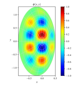
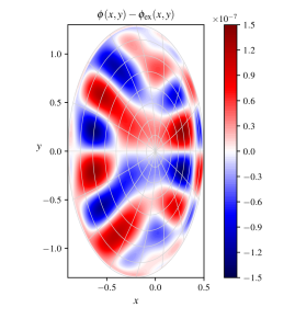
Figure 4: Numerical solution of Poisson’s equation on a disk-like domain defined by mapping (2) with the parameters in (4): contour plots of the numerical solution (left) and error (right), obtained with $n_{1}\times n_{2}=128\times 256$ and cubic splines.

$n_{1}\times n_{2}$	$||\Delta\phi||_{L^{2}}$	Order	$||\Delta\phi||_{L^{\infty}}$	Order
$32\times 64$	$7.10\times 10^{-5}$		$4.17\times 10^{-5}$
$64\times 128$	$3.87\times 10^{-6}$	$4.20$	$2.31\times 10^{-6}$	$4.17$
$128\times 256$	$2.33\times 10^{-7}$	$4.05$	$1.41\times 10^{-7}$	$4.03$
$256\times 512$	$1.44\times 10^{-8}$	$4.02$	$8.78\times 10^{-9}$	$4.01$
$512\times 1024$	$8.99\times 10^{-10}$	$4.00$	$5.48\times 10^{-10}$	$4.00$

Table 3: Numerical solution of Poisson’s equation on a disk-like domain defined by mapping (2) with the parameters in (4): fourth-order convergence of the solver using cubic splines.

5.4 Evaluation of the electric field

The advection fields for the transport of $\rho$ in the guiding-center model (1) are obtained from the potential $\phi$ by means of derivatives. This section suggests a strategy to evaluate the Cartesian components of the gradient of $\widehat{\phi}$ while taking into account the singularity at the pole. We denote again by $\widehat{\boldsymbol{\nabla}}\widehat{\phi}$ the gradient of $\widehat{\phi}$ in the logical domain. The Cartesian components of the gradient are obtained from the logical ones by applying the inverse of the transposed Jacobian matrix:

$$\boldsymbol{\nabla}\widehat{\phi}(s,\theta)=(J_{\boldsymbol{F}}^{-1})^{T}(s,\theta)\,\widehat{\boldsymbol{\nabla}}{\widehat{\phi}}(s,\theta)\,.$$ (29)

From an analytical point of view, (29) holds for all values of $s>0$ and its limit as $s\to 0^{+}$ is finite and unique. From a numerical point of view, (29) holds for all values of $s$ sufficiently far from the pole, as far as the inverse Jacobian does not become too large. Therefore, we assume that (29) holds for $s\geq\epsilon$, for a given small $\epsilon$. For $s=0$ the partial derivative with respect to $\theta$ vanishes and all the information is contained in the partial derivative with respect to $s$, which takes a different value for each value of $\theta$. Recalling that a partial derivative has the geometrical meaning of a directional derivative along a vector of the tangent basis, the idea is to combine two given values corresponding to two different values of $\theta$ and extract from them the Cartesian components of the gradient at the pole. The two chosen values of $\theta$ must correspond to linearly independent directions, so that from

$$\frac{\partial\widehat{\phi}}{\partial s}(0,\theta_{1})=\boldsymbol{\nabla}\widehat{\phi}\cdot\boldsymbol{e}_{s}=(\boldsymbol{\nabla}\widehat{\phi})_{x}\frac{\partial x}{\partial s}(0,\theta_{1})+(\boldsymbol{\nabla}\widehat{\phi})_{y}\frac{\partial y}{\partial s}(0,\theta_{1})\,,$$

$$\frac{\partial\widehat{\phi}}{\partial s}(0,\theta_{2})=\boldsymbol{\nabla}\widehat{\phi}\cdot\boldsymbol{e}_{s}=(\boldsymbol{\nabla}\widehat{\phi})_{x}\frac{\partial x}{\partial s}(0,\theta_{2})+(\boldsymbol{\nabla}\widehat{\phi})_{y}\frac{\partial y}{\partial s}(0,\theta_{2})\,,$$

the two components $(\boldsymbol{\nabla}\widehat{\phi})_{x}$ and $(\boldsymbol{\nabla}\widehat{\phi})_{y}$ can be obtained. Each possible couple of linearly independent directions produces the same result. In order to connect the two approaches in a smooth way, for $0<s<\epsilon$ we interpolate linearly the value at the pole $s=0$ and the value at $s=\epsilon$:

$$\boldsymbol{\nabla}\widehat{\phi}(s,\theta)=\bigg{(}1-\frac{s}{\epsilon}\bigg{)}\boldsymbol{\nabla}\widehat{\phi}(0,\theta)+\frac{s}{\epsilon}\boldsymbol{\nabla}\widehat{\phi}(\epsilon,\theta)\,.$$

We remark that the parameter $\epsilon$ can be chosen arbitrarily small, as far as it avoids underflows and overflows in floating point arithmetic. For all the numerical tests discussed in this work we set $\epsilon=10^{-12}$.

6 Self-consistent test cases: the guiding-center model

We now address the solution of the guiding-center model

$$\begin{cases}\dfrac{\partial\rho}{\partial t}-E^{y}\dfrac{\partial\rho}{\partial x}+E^{x}\dfrac{\partial\rho}{\partial y}=0\,,\\[5.69054pt] -\boldsymbol{\nabla}\cdot\boldsymbol{\nabla}\phi=\rho\,,\end{cases}\quad\textrm{with}\quad\begin{cases}\rho(0,x,y)=\rho_{\text{IN}}(x,y)\,,\\[5.69054pt] \phi(t,x,y)=0\textrm{ on }\partial\Omega\,.\end{cases}$$ (30)

Physical quantities conserved by the model are the total mass and energy

$$\mathcal{M}(t):= \int_{\Omega}\textrm{d}x\,\textrm{d}y\,\rho(t,x,y) =\int_{\widehat{\Omega}}\textrm{d}s\,\textrm{d}\theta\,|\det J_{\boldsymbol{F}}(s,\theta)|\,\widehat{\rho}(t,s,\theta)\,,$$ (31)

$$\mathcal{W}(t):= \int_{\Omega}\textrm{d}x\,\textrm{d}y\,|\boldsymbol{E}(t,x,y)|^{2} =\int_{\widehat{\Omega}}\textrm{d}s\,\textrm{d}\theta\,|\det J_{\boldsymbol{F}}(s,\theta)|\,|\widehat{\boldsymbol{E}}(t,s,\theta)|^{2}\,.$$

These integrals are computed using the Gauss-Legendre quadrature points and weights mentioned in section 3. We define the relative errors for the conservation of the invariants (31) as

$$\delta\mathcal{M}(t):=\frac{|\mathcal{M}(0)-\mathcal{M}(t)|}{|\mathcal{M}(0)|}\,,\quad\delta\mathcal{W}(t):=\frac{|\mathcal{W}(0)-\mathcal{W}(t)|}{|\mathcal{W}(0)|}\,.$$ (32)

Before describing the numerical tests considered for this model, we present our time-advancing strategy and how we deal with the problem of defining an equilibrium density on complex mappings while initializing our simulations.

6.1 Time integration

We present here two different time integration schemes, one explicit and one implicit, that may be chosen according to the particular physical dynamics described by model (30). Both integration schemes are based on a predictor-corrector procedure. In the numerical tests discussed in this section, the explicit scheme is our default choice, because of its low computational cost. However, there are situations (as, for example, the test case simulating the merger of two macroscopic vortices presented in section 6.4) where the dynamics described by model (30) is such that the explicit scheme would require very small time steps in order to produce correct results. Instead, the implicit trapezoidal scheme that we describe here has proven capable of capturing the correct dynamics with much larger time steps, thanks to its symmetry and adjoint-symplecticity [36].

6.1.1 Second-order explicit scheme

The explicit time integration scheme is the second-order integrator described in [37, section 2.2]. Since it will be used also for test cases involving point charges, we denote here again by $\rho_{\text{SL}}$ and $\rho_{\text{PIC}}$ the semi-Lagrangian density and the particle density, respectively. Moreover, following the notation of section 4, we denote by $\boldsymbol{X}_{ij}:=\boldsymbol{G}(\boldsymbol{\eta}_{ij})$ the pseudo-Cartesian coordinates of a given mesh point and by $\boldsymbol{X}_{c}:=\boldsymbol{G}(\boldsymbol{\eta}_{c})$ the pseudo-Cartesian coordinates of a given point charge, respectively. The first-order prediction (superscript “$(P)$”) is given by

$$\accentset{\mbox{\Large\hskip 1.54999pt.}}{\boldsymbol{X}}_{ij}^{(P)}:=(J_{\boldsymbol{F}}J_{\boldsymbol{G}}^{-1})^{-1}(\boldsymbol{\eta}_{ij})\,\widehat{\boldsymbol{A}}(\boldsymbol{\eta}_{ij}) \,,\quad \boldsymbol{X}_{ij}^{(P)}:=\boldsymbol{X}_{ij}-\Delta t\,\accentset{\mbox{\Large\hskip 1.54999pt.}}{\boldsymbol{X}}_{ij}^{(P)} \,,\quad \boldsymbol{\eta}_{ij}^{(P)}:=\boldsymbol{G}^{-1}(\boldsymbol{X}_{ij}^{(P)})\,;$$

$$\accentset{\mbox{\Large\hskip 1.54999pt.}}{\boldsymbol{X}}_{c}^{(P)}:=(J_{\boldsymbol{F}}J_{\boldsymbol{G}}^{-1})^{-1}(\boldsymbol{\eta}_{c})\,\widehat{\boldsymbol{A}}(\boldsymbol{\eta}_{c}) \,,\quad \boldsymbol{X}_{c}^{(P)}:=\boldsymbol{X}_{c}+\Delta t\,\accentset{\mbox{\Large\hskip 1.54999pt.}}{\boldsymbol{X}}_{c}^{(P)} \,,\quad \boldsymbol{\eta}_{c}^{(P)}:=\boldsymbol{G}^{-1}(\boldsymbol{X}_{c}^{(P)})\,.$$

We then compute the intermediate semi-Lagrangian and particle densities $\rho^{(P)}_{\text{SL}}$ and $\rho^{(P)}_{\text{PIC}}$ and obtain the intermediate electric potential $\phi^{(P)}$ by solving Poisson’s equation. Denoting by $\widehat{\boldsymbol{A}}^{(P)}$ the corresponding intermediate advection field, the second-order correction (superscript “$(C)$”) is given by

$$\accentset{\mbox{\Large\hskip 1.54999pt.}}{\boldsymbol{X}}_{ij}^{(C)}:=(J_{\boldsymbol{F}}J_{\boldsymbol{G}}^{-1})^{-1}(\boldsymbol{\eta}_{ij}^{(P)})\,\widehat{\boldsymbol{A}}(\boldsymbol{\eta}_{ij}^{(P)})+(J_{\boldsymbol{F}}J_{\boldsymbol{G}}^{-1})^{-1}(\boldsymbol{\eta}_{ij})\,\widehat{\boldsymbol{A}}^{(P)}(\boldsymbol{\eta}_{ij}) \,,\quad \boldsymbol{X}_{ij}^{(C)}:=\boldsymbol{X}_{ij}-\frac{\Delta t}{2}\accentset{\mbox{\Large\hskip 1.54999pt.}}{\boldsymbol{X}}_{ij}^{(C)} \,,\quad \boldsymbol{\eta}_{ij}^{(C)}:=\boldsymbol{G}^{-1}(\boldsymbol{X}_{ij}^{(C)})\,;$$

$$\accentset{\mbox{\Large\hskip 1.54999pt.}}{\boldsymbol{X}}_{c}^{(C)}:=(J_{\boldsymbol{F}}J_{\boldsymbol{G}}^{-1})^{-1}(\boldsymbol{\eta}_{c})\,\widehat{\boldsymbol{A}}(\boldsymbol{\eta}_{c})+(J_{\boldsymbol{F}}J_{\boldsymbol{G}}^{-1})^{-1}(\boldsymbol{\eta}_{c}^{(P)})\,\widehat{\boldsymbol{A}}^{(P)}(\boldsymbol{\eta}_{c}^{(P)}) \,,\quad \boldsymbol{X}_{c}^{(C)}:=\boldsymbol{X}_{c}+\frac{\Delta t}{2}\accentset{\mbox{\Large\hskip 1.54999pt.}}{\boldsymbol{X}}_{c}^{(C)} \,,\quad \boldsymbol{\eta}_{c}^{(C)}:=\boldsymbol{G}^{-1}(\boldsymbol{X}_{c}^{(C)})\,.$$

For point charges, this second-order scheme is equivalent to Heun’s method (improved Euler’s method [38]).

6.1.2 Second-order implicit scheme

The implicit time integration scheme is based on the implicit trapezoidal rule and it will not be used for test cases involving point charges. We denote again by $\rho_{\text{SL}}$ the semi-Lagrangian density and by $\boldsymbol{X}_{ij}:=\boldsymbol{G}(\boldsymbol{\eta}_{ij})$ the pseudo-Cartesian coordinates of a given mesh point. The second-order prediction (superscript “$(P)$”) is given by $\boldsymbol{X}_{ij}^{(P)}:=\boldsymbol{X}_{ij}^{(k)}$ and ${\boldsymbol{\eta}_{ij}^{(P)}:=\boldsymbol{G}^{-1}(\boldsymbol{X}_{ij}^{(P)})}$, where the $k$-th iteration is computed as

$$\accentset{\mbox{\Large\hskip 1.54999pt.}}{\boldsymbol{X}}_{ij}^{(k)}:=(J_{\boldsymbol{F}}J_{\boldsymbol{G}}^{-1})^{-1}(\boldsymbol{\eta}_{ij})\,\widehat{\boldsymbol{A}}(\boldsymbol{\eta}_{ij})+(J_{\boldsymbol{F}}J_{\boldsymbol{G}}^{-1})^{-1}(\boldsymbol{\eta}_{ij}^{(k-1)})\,\widehat{\boldsymbol{A}}(\boldsymbol{\eta}_{ij}^{(k-1)})\,,\quad\boldsymbol{X}_{ij}^{(k)}:=\boldsymbol{X}_{ij}-\frac{\Delta t}{4}\accentset{\mbox{\Large\hskip 1.54999pt.}}{\boldsymbol{X}}_{ij}^{(k)}\,,\quad\boldsymbol{\eta}_{ij}^{(k)}:=\boldsymbol{G}^{-1}(\boldsymbol{X}_{ij}^{(k)})\,,$$

with $\boldsymbol{X}_{ij}^{(0)}:=\boldsymbol{X}_{ij}$ and $\boldsymbol{\eta}_{ij}^{(0)}:=\boldsymbol{\eta}_{ij}$, provided that $|\boldsymbol{X}_{ij}^{(k)}-\boldsymbol{X}_{ij}^{(k-1)}|^{2}\leq\tau^{2}$, where the tolerance $\tau$ is defined as ${\tau:=\tau_{A}+\tau_{R}\,|\boldsymbol{X}_{ij}|}$, for given absolute and relative tolerances $\tau_{A}$ and $\tau_{R}$. We then compute the intermediate semi-Lagrangian density $\rho^{(P)}_{\text{SL}}$ and obtain the intermediate electric potential $\phi^{(P)}$ by solving Poisson’s equation. Denoting by $\widehat{\boldsymbol{A}}^{(P)}$ the corresponding intermediate advection field, the second-order correction (superscript “$(C)$”) is given by $\boldsymbol{X}_{ij}^{(C)}:=\boldsymbol{X}_{ij}^{(k)}$ and ${\boldsymbol{\eta}_{ij}^{(C)}:=\boldsymbol{G}^{-1}(\boldsymbol{X}_{ij}^{(C)})}$, where the $k$-th iteration is computed as

$$\accentset{\mbox{\Large\hskip 1.54999pt.}}{\boldsymbol{X}}_{ij}^{(k)}:=(J_{\boldsymbol{F}}J_{\boldsymbol{G}}^{-1})^{-1}(\boldsymbol{\eta}_{ij})\,\widehat{\boldsymbol{A}}^{(P)}(\boldsymbol{\eta}_{ij})+(J_{\boldsymbol{F}}J_{\boldsymbol{G}}^{-1})^{-1}(\boldsymbol{\eta}_{ij}^{(k-1)})\,\widehat{\boldsymbol{A}}^{(P)}(\boldsymbol{\eta}_{ij}^{(k-1)})\,,\quad\boldsymbol{X}_{ij}^{(k)}:=\boldsymbol{X}_{ij}-\frac{\Delta t}{2}\accentset{\mbox{\Large\hskip 1.54999pt.}}{\boldsymbol{X}}_{ij}^{(k)}\,,\quad\boldsymbol{\eta}_{ij}^{(k)}:=\boldsymbol{G}^{-1}(\boldsymbol{X}_{ij}^{(k)})\,,$$

with $\boldsymbol{X}_{ij}^{(0)}:=\boldsymbol{X}_{ij}$ and $\boldsymbol{\eta}_{ij}^{(0)}:=\boldsymbol{\eta}_{ij}$, provided that $|\boldsymbol{X}_{ij}^{(k)}-\boldsymbol{X}_{ij}^{(k-1)}|^{2}\leq\tau^{2}$.

6.2 Numerical equilibria

Defining an equilibrium density $\rho$ and a corresponding equilibrium potential $\phi$ for the system (30) becomes non-trivial on domains defined by complex non-circular mappings, such as (2) and (3). In the case of circular mappings, any axisymmetric density independent of the angle variable $\theta$ turns out to be an equilibrium for the transport equation in (30). For more complex mappings we follow the numerical procedure suggested in [39], and references therein, to compute an equilibrium couple $(\rho,\phi)$. The equilibrium is determined by the eigenvalue problem of finding $(\sigma,\phi)$ such that $-\boldsymbol{\nabla}\cdot\boldsymbol{\nabla}\phi=\sigma\,f(\phi)$, with given $f$ such that $f^{\prime}(\phi)\neq 0$ in some limited domain. Given initial data $(\sigma^{(0)},\phi^{(0)})$, the $i$-th iteration, with $i\geq 1$, is computed with the following steps:

1. compute $\rho^{(i)}:=\sigma^{(i-1)}f(\phi^{(i-1)})$;

2. compute $\phi^{(i)}_{*}$ by solving $-\boldsymbol{\nabla}\cdot\boldsymbol{\nabla}\phi^{(i)}_{*}=\rho^{(i)}$;

3. if a maximum value $\phi_{\text{max}}$ is given, compute $c^{(i)}$ by setting $c^{(i)}:=\phi_{\text{max}}/||\phi^{(i)}_{*}||_{L^{\infty}}$;
   if a maximum value $\rho_{\text{max}}$ is given, compute $c^{(i)}$ by solving ${c^{(i)}f(c^{(i)}\,||\phi^{(i)}_{*}||_{L^{\infty}})=\rho_{\text{max}}/\sigma^{(i-1)}}$;

4. compute $(\sigma^{(i)},\phi^{(i)}):=c^{(i)}\,(\sigma^{(i-1)},\phi^{(i)}_{*})$.

The iterative procedure stops when $|\sigma^{(i)}-\sigma^{(i-1)}|\leq\tau$, for a given tolerance $\tau$. The eigenvalue problem does not have a unique solution, but the algorithm is expected to converge to the ground state, that is, the eigenstate with minimum eigenvalue. Figure 5 illustrates, for example, the equilibrium obtained in this way for $f(\phi)=\phi^{2}$ and $\rho_{\text{max}}=1$ on domains defined by a circular mapping and by mapping (3) with the parameters in (5).

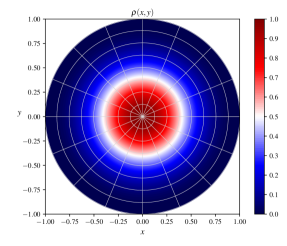
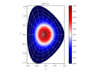
Figure 5: Numerical equilibrium density $\rho$ obtained with $f(\phi)=\phi^{2}$ and $\rho_{\text{max}}=1$ on disk-like domains defined by a circular mapping (left) and by mapping (3) with the parameters in (5) (right).

6.3 Numerical test: diocotron instability

As a first test we investigate the evolution of the diocotron instability on a domain defined by a circular mapping. From a physical point of view, this corresponds to studying a non-neutral plasma in cylindrical geometry, where the plasma particles are confined radially by a uniform axial magnetic field with a cylindrical conducting wall located at the outer boundary [40]. Following [4], we consider the initial density profile

$$\widehat{\rho}(0,s,\theta):=\widehat{\rho}_{0}(s)+\widehat{\rho}_{1}(0,s,\theta):=\begin{dcases}1+\epsilon\cos(m\,\theta)&s^{-}\leq s\leq s^{+}\,,\\ 0&\text{elsewhere}\,.\end{dcases}$$ (33)

This corresponds to a $\theta$-independent equilibrium $\widehat{\rho}_{0}$ (an annular charged layer) with a density perturbation $\widehat{\rho}_{1}$ of azimuthal mode number $m$ and small amplitude $\epsilon$. The linear dispersion relation for a complex eigenfrequency $\omega$ reads [4]

$$\left(\frac{\omega}{\omega_{D}}\right)^{2}-b_{m}\frac{\omega}{\omega_{D}}+c_{m}=0\,,$$ (34)

where $\omega_{D}$ is the diocotron frequency ($\omega_{D}=1/2$ in our units), and $b_{m}$ and $c_{m}$ are defined as

$$b_{m}:=m\left[1-\left(\frac{s^{-}}{s^{+}}\right)^{2}\right]+(s^{+})^{2m}-(s^{-})^{2m}\,,$$

$$c_{m}:=m\left[1-\left(\frac{s^{-}}{s^{+}}\right)^{2}\right]\left[1-(s^{-})^{2m}\right]-\left[1-\left(\frac{s^{-}}{s^{+}}\right)^{2m}\right]\left[1-(s^{+})^{2m}\right]\,.$$

If $4c_{m}>b_{m}^{2}$, then the oscillation frequencies resulting from (34) form complex conjugate pairs. The solution with $\text{Im}\,\omega>0$ corresponds to the diocotron instability and describes how rapidly the electric potential grows. The quantity of interest, in this regard, is the $L^{2}$-norm of the perturbed electric potential

$$||\phi-\phi_{0}||_{L^{2}}:=\sqrt{\int_{\Omega}\textrm{d}x\,\textrm{d}y\,\left[\phi(t,x,y)-\phi_{0}(x,y)\right]^{2}}=\sqrt{\int_{\widehat{\Omega}}\textrm{d}s\,\textrm{d}\theta\,|\det J_{\boldsymbol{F}}(s,\theta)|\,\left[\widehat{\phi}(t,s,\theta)-\widehat{\phi}_{0}(s,\theta)\right]^{2}}\,,$$

where $\phi_{0}$ denotes the equilibrium electric potential and the integration is performed again on the Gauss-Legendre quadrature points and weights. In order to represent the initial density in the finite-dimensional space of tensor-product splines, we modify (33) by a radial smoothing to avoid discontinuities:

$$\widehat{\rho}(0,s,\theta):=\widehat{\rho}_{0}(s)+\widehat{\rho}_{1}(0,s,\theta):=\begin{dcases}\left[1+\epsilon\cos(m\,\theta)\right]\exp\left[-\left(\frac{s-\widebar{s}}{d}\right)^{p}\right]&s^{-}\leq s\leq s^{+}\,,\\ 0&\text{elsewhere}\,,\end{dcases}$$ (35)

with $\widebar{s}:=(s^{+}+s^{-})/2$ and $d:=(s^{+}-s^{-})/2$. If the smoothing layer is small enough, we can still rely on the analytical result obtained for the dispersion relation in the case of the sharp annular layer (33). The numerical results have been verified against the analytical dispersion relation for a perturbation with azimuthal mode number $m=9$ and amplitude $\epsilon=10^{-4}$. The numerical growth rate is in good agreement with the analytical one, $\text{Im}\,\omega\approx 0.18$, for the time interval $20\lesssim t\lesssim 50$, which corresponds to the linear phase. At time $t\approx 50$, the system enters its non-linear phase. The simulation is run with $n_{1}\times n_{2}=128\times 256$ and $\Delta t=0.1$, with the explicit time integrator described in section 6.1.1. Additional parameters defining the initial condition (35) have been set to $s^{-}=0.45$, $s^{+}=0.50$ and $p=50$. Numerical results are illustrated in Figures 6 and 7.

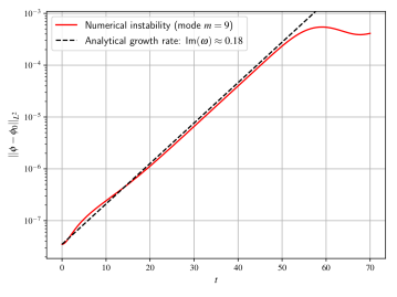
Figure 6: Numerical simulation of the diocotron instability: $L^{2}$-norm of the perturbed electric potential.

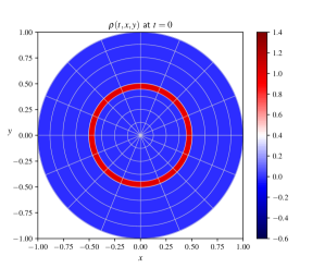
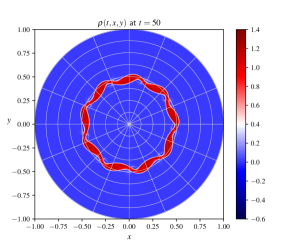
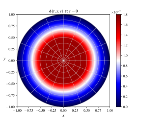
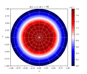
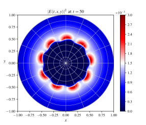
Figure 7: Numerical simulation of the diocotron instability. From left to right, from top to bottom: contour plots of the density $\rho(t,x,y)$, the electric potential $\phi(t,x,y)$ and the electric energy density $|\boldsymbol{E}(t,x,y)|^{2}$ at times $t=0$ (beginning of the simulation) and $t=50$ (end of the linear phase).

For the conservation of mass and energy we get

$$\max_{t\in[0,70]}\delta\mathcal{M}(t)\approx 5.8\times 10^{-4}\,,\quad\max_{t\in[0,70]}\delta\mathcal{W}(t)\approx 1.8\times 10^{-3}\,.$$

The time evolution of the relative errors on these conserved quantities is shown in Figure 8.

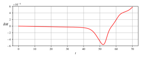
Figure 8: Numerical simulation of the diocotron instability: time evolution of the relative errors on the total mass (left) and energy (right).

Figure 7 shows that in this test case nothing significant happens in the region close to the pole. The effect of using $\mathcal{C}^{1}$ smooth polar splines in such situations is not particularly evident, but they do ensure continuity of the advection field responsible for the transport of $\rho$ (the electric field) everywhere in the domain. Moreover, pseudo-Cartesian coordinates reduce to standard Cartesian coordinates, as the physical domain is defined by a simple circular mapping. The interest of this test case lies primarily in the fact that it provides the valuable possibility of easily verifying the implementation of our numerical scheme by comparing the numerical results with an analytical dispersion relation.

6.4 Numerical test: vortex merger

In the context of incompressible inviscid 2D Euler fluids, we simulate the merger of two macroscopic vortices by setting up initial conditions qualitatively similar to those described in [5, section 3]. Unlike the diocotron instability, the interest of this test case lies primarily in the fact that the relevant dynamics occurs in a region close to the pole of the physical domain. We consider an equilibrium $\rho_{0}$ obtained with the numerical procedure described in section 6.2 with $f(\phi)=\phi^{2}$ and $\phi_{\text{max}}=1$, and perturb it with two Gaussian perturbations,

$$\begin{split}\rho(0,x,y)&:=\rho_{0}(x,y)+\rho_{1}(0,x,y)\\ &:=\rho_{0}(x,y)+\epsilon\left(\exp\left[-\frac{(x-x^{*}_{1})^{2}+(y-y^{*}_{1})^{2}}{2\sigma^{2}}\right]+\exp\left[-\frac{(x-x^{*}_{2})^{2}+(y-y^{*}_{2})^{2}}{2\sigma^{2}}\right]\,\right)\,,\end{split}$$

with amplitude $\epsilon=10^{-4}$, width $\sigma=0.08$ and centered in $(x^{*}_{1},y^{*}_{1})=(+0.08,-0.14)$ and $(x^{*}_{2},y^{*}_{2})=(-0.08,+0.14)$. The time evolution of the initial perturbation $\rho_{1}$ is shown in Figure 9. The simulation is run with ${n_{1}\times n_{2}=128\times 256}$ and time step $\Delta t=0.1$, with the second-order implicit time integrator described in section 6.1.2. The explicit time integrator would require in this case very small time steps in order to capture the correct dynamics. Two different aspects play a role in the choice of the time integrator for this particular test case. On the one hand, the error in the integration of the characteristics, which scales with $\Delta t^{2}$ for the second-order explicit scheme described in section 6.1.1, must not be larger than the amplitude of the perturbation on the advection field caused by the density perturbation. In other words, for the explicit scheme, the choice of the time step would be dependent on the amplitude $\epsilon$ of the density perturbation. On the other hand, committing an error in the integration of closed trajectories (as it would be when using the explicit scheme even for stationary advection fields) seems to disrupt the dynamics, preventing the simulation from correctly predicting the merger of the two macroscopic vortices. For the conservation of mass and energy we get

$$\max_{t\in[0,10]}\delta\mathcal{M}(t)\approx 2.8\times 10^{-9}\,,\quad\max_{t\in[0,10]}\delta\mathcal{W}(t)\approx 4.9\times 10^{-9}\,.$$

The time evolution of the relative errors on these conserved quantities is shown in Figure 10. The results of a convergence analysis of the numerical results while decreasing the time step are shown in Table 4, where $\Delta\rho$ denotes the difference between the vorticity $\rho$ and a reference vorticity obtained by running a simulation with time step $\Delta t=0.1/16$.

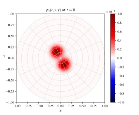
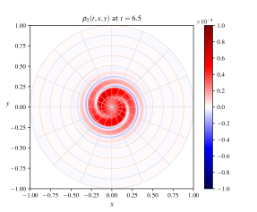
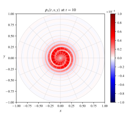
Figure 9: Numerical simulation of the merger of two vortices: contour plots of the vorticity perturbation $\rho_{1}(t,x,y)$ at different times.

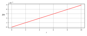
Figure 10: Numerical simulation of the merger of two vortices: time evolution of the relative errors on the total mass (left) and energy (right).

$\Delta t$	$||\Delta\rho||_{L^{\infty}}$	Order	$\max_{t}\delta\mathcal{M}(t)$	Order	$\max_{t}\delta\mathcal{W}(t)$	Order
$0.1$	$3.04\times 10^{-5}$		$2.84\times 10^{-9}$		$4.92\times 10^{-9}$
$0.1/2$	$8.44\times 10^{-6}$	$1.85$	$1.42\times 10^{-9}$	$1.00$	$2.47\times 10^{-9}$	$0.99$
$0.1/4$	$2.05\times 10^{-6}$	$2.04$	$7.14\times 10^{-10}$	$0.99$	$1.22\times 10^{-9}$	$1.02$
$0.1/8$	$4.12\times 10^{-7}$	$2.32$	$3.46\times 10^{-10}$	$1.05$	$6.08\times 10^{-10}$	$1.01$

Table 4: Convergence in time of the numerical results for the vortex merger with respect to reference results obtained with time step $\Delta t=0.1/16$. The mesh size $n_{1}\times n_{2}=128\times 256$ is kept fixed in this convergence analysis.

6.5 Numerical test: point-like vortex dynamics

We also investigate the dynamics of point-like vortices (or point charges) on a non-uniform equilibrium, following the discussion in [11]. The numerical tests presented in this section show that the numerical approaches suggested in this work can be applied straightforwardly in the context of particle-in-cell methods. This makes our numerical strategy interesting also for numerical codes based on such methods, as for example many codes developed for the simulation of turbulence in magnetized fusion plasmas by means of gyrokinetic models [41, 42, 43, 44]. The examples discussed here can be considered as limit cases of usual particle-in-cell simulations, as we will include only one single point-like vortex (or point charge) in the system. Since our strategy turns out to work well for this extreme scenario, we do not expect issues when dealing with the usual case of large numbers of particles. The point-like vortex contributes to the total charge density as described in equation (24). Moreover, the position of the point-like vortex is evolved following the same advection field $(-E^{y},E^{x})^{T}$ responsible for the transport of $\rho$. Integration in time is performed with the second-order explicit scheme described in section 6.1.1. For a domain defined by a circular mapping, we consider an equilibrium vorticity of the form

$$\widehat{\rho}_{0}(s):=\begin{dcases}1-1.25\,s&s\leq 0.8\,,\\ 0&s>0.8\,,\end{dcases}$$

identical to the one considered in [11, section IV]. Figure 11 shows the local stream lines of the advection field near positive and negative point-like vortices at the initial time in a rotating frame where the point-like vortices are initially at rest. This is obtained in practice by rotating given coordinates $(x,y)$ at time $t$ as

$$x^{\prime}:=x\cos(-\omega t)-y\sin(-\omega t)\,,$$

$$y^{\prime}:=x\sin(-\omega t)+y\cos(-\omega t)\,,$$

and by transforming the advection field $(-E^{y},E^{x})^{T}$ to the rotated field $(E^{y}+\omega\,y,E^{x}-\omega\,x)^{T}$, where $\omega=0.3332$ represents the angular velocity of the background at $t=0$ and $s=0.4$.

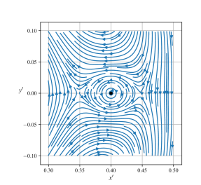
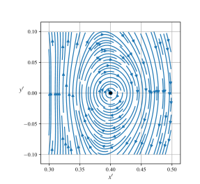
Figure 11: Local stream lines of the advection field near positive (left) and negative (right) point-like vortices in a rotating frame $(x^{\prime},y^{\prime})$.

Figure 12 shows results for a point-like vortex of intensity $q=\pm 0.0025$ at the initial position $s=0.4$ and $\theta=0$, again viewed in a rotating frame. Time is here normalized as $t^{\prime}=0.1668\,t$ (as in [11], where $t^{\prime}$ is denoted as $T$). The results shown in Figure 12 are in agreement with the ones shown in Figures 7a and 10a of [11].

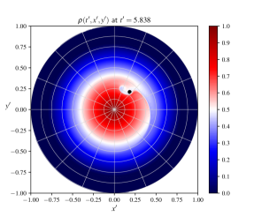
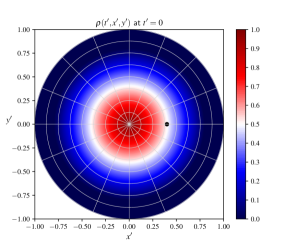
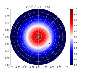
Figure 12: Dynamics of a positive (top) and negative (bottom) point-like vortex on a domain defined by a circular mapping: contour plots of the vorticity at times $t^{\prime}=0$ and $t^{\prime}=5.838$ in a rotating frame $(x^{\prime},y^{\prime})$.

As explained in [11], positive point-like vortices drift transverse to the shear flow, up the background vorticity gradient, while negative point-like vortices drift down the gradient. Figure 13 shows the time evolution of the radial position of the vortices, in agreement with the results shown in Figures 7b and 10b of [11].

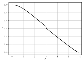
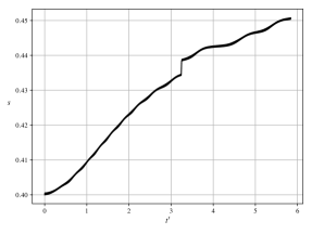
Figure 13: Time evolution of the radial position of a positive (left) and negative (right) point-like vortex.

The simulation is run with $n_{1}\times n_{2}=256\times 512$ and time step $\Delta t=0.005$. The time step is chosen small enough to resolve the oscillations due to the self-force experienced by the point-like vortices. Moreover, the computational mesh needs to be finer than the previous test cases in order to capture correctly the complex nonlinear dynamics of the interaction between the point-like vortices and the background vorticity. For a rough comparison, the vortex-in-cell simulations discussed in [11] require as well a large computational rectangular grid of size $1025\times 1025$. Special techniques may be used to reduce self-force effects on non-uniform meshes (or even unstructured meshes) [45], but they are not considered in this work. For the conservation of mass and energy we get

$$\max_{t^{\prime}\in[0,5.838]}\delta\mathcal{M}(t^{\prime})\approx 6.9\times 10^{-6}\,,\quad\max_{t^{\prime}\in[0,5.838]}\delta\mathcal{W}(t^{\prime})\approx 8.4\times 10^{-3}$$

for the positive point-like vortex and

$$\max_{t^{\prime}\in[0,5.838]}\delta\mathcal{M}(t^{\prime})\approx 6.9\times 10^{-6}\,,\quad\max_{t^{\prime}\in[0,5.838]}\delta\mathcal{W}(t^{\prime})\approx 7.3\times 10^{-3}$$

for the negative point-like vortex. The time evolution of the relative errors on these conserved quantities is shown in Figure 14.

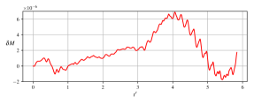
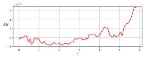
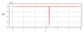
Figure 14: Dynamics of a positive (top) and negative (bottom) point-like vortex on a domain defined by a circular mapping: time evolution of the relative errors on the total mass (left) and energy (right).

Similar simulations on mapping (3), initialized with an equilibrium vorticity obtained with the numerical procedure described in section 6.2 with $f(\phi)=\phi^{2}$ and $\rho_{\text{max}}=1$, show the same qualitative behavior: a positive point-like vortex drifts towards the center of the domain, while a negative point-like vortex drifts towards the boundary (Figure 15). The final time $t=35$ corresponds to the normalized time $t^{\prime}=5.838$ considered before.

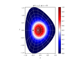
Figure 15: Dynamics of a positive (top) and negative (bottom) point-like vortex on a disk-like domain defined by mapping (3) with the parameters in (5): contour plots of the vorticity at times $t=0$ and $t=35$.

For the conservation of mass and energy we get

$$\max_{t\in[0,35]}\delta\mathcal{M}(t)\approx 1.6\times 10^{-5}\,,\quad\max_{t\in[0,35]}\delta\mathcal{W}(t)\approx 6.9\times 10^{-3}$$

for the positive point-like vortex and

$$\max_{t\in[0,35]}\delta\mathcal{M}(t)\approx 3.6\times 10^{-6}\,,\quad\max_{t\in[0,35]}\delta\mathcal{W}(t)\approx 5.7\times 10^{-3}$$

for the negative point-like vortex. The time evolution of the relative errors on these conserved quantities is shown in Figure 16.

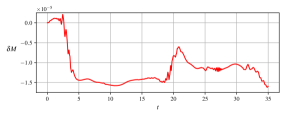
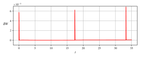
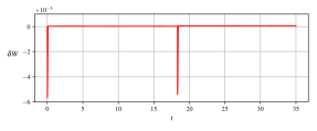
Figure 16: Dynamics of a positive (top) and negative (bottom) point-like vortex on a disk-like domain defined by mapping (3) with the parameters in (5): time evolution of the relative errors on the total mass (left) and energy (right).

7 Conclusions and outlook

We presented a comprehensive numerical strategy for the solution of systems of coupled hyperbolic and elliptic partial differential equations on disk-like domains with a singularity at a unique pole, where one edge of the rectangular logical domain collapses to one point of the physical domain. We introduced a novel set of coordinates, named pseudo-Cartesian coordinates, for the integration of the characteristics of the hyperbolic equation of the system. Such coordinates are well-defined everywhere in the computational domain, including the pole, and provide a straightforward and relatively simple solution for dealing with singularities while solving advection problems in complex geometries. They reduce to standard Cartesian coordinates in the case of a circular mapping. Moreover, we developed a finite element elliptic solver based on globally $\mathcal{C}^{1}$ smooth splines [27]. In this work we considered only $\mathcal{C}^{1}$ smoothness, but higher-order smoothness, consistent with the spline degree, may be considered as well. We tested our solvers on several test cases in the simplest case of a circular domain and in more complex geometries. The numerical methods presented here show high-order convergence in the space discretization parameters, uniformly across the computational domain, including the pole. Moreover, the techniques discussed can be easily applied in the context of particle-in-cell methods and are not necessarily restricted to semi-Lagrangian schemes, which were here discussed in more detail. The range of physical problems that can be approached following the ideas presented in this work includes the study of turbulence in magnetized fusion plasmas by means of Vlasov-Poisson fully kinetic models as well as drift-kinetic and gyrokinetic models, and turbulence models for incompressible inviscid Euler fluids in the context of fluid dynamics.

References

- Tan and Shu [2010] S. Tan and C. Shu. Inverse Lax-Wendroff procedure for numerical boundary conditions of conservation laws. Journal of Computational Physics, 229(21):8144–8166, 2010. doi:https://doi.org/10.1016/j.jcp.2010.07.014.
- O’Neil [1985] T.M. O’Neil. New Theory of Transport Due to Like-Particle Collisions. Phys. Rev. Lett., 55:943–946, 1985. doi:10.1103/PhysRevLett.55.943.
- Dubin and O’Neil [1988] D.H.E. Dubin and T.M. O’Neil. Two-dimensional guiding-center transport of a pure electron plasma. Phys. Rev. Lett., 60:1286–1289, 1988. doi:10.1103/PhysRevLett.60.1286.
- Davidson [2001] R.C. Davidson. Physics of Nonneutral Plasmas. Co-published with World Scientific Publishing Co., 2001. doi:10.1142/p251.
- Driscoll et al. [2002] C.F. Driscoll, D.Z. Jin, D.A. Schecter, and D.H.E. Dubin. Vortex dynamics of 2D electron plasmas. Physica C: Superconductivity, 369(1):21–27, 2002. doi:10.1016/S0921-4534(01)01216-3.
- Sengupta and Ganesh [2014] M. Sengupta and R. Ganesh. Inertia driven radial breathing and nonlinear relaxation in cylindrically confined pure electron plasma. Physics of Plasmas, 21(2), 2014. doi:10.1063/1.4866022.
- Sengupta and Ganesh [2015] M. Sengupta and R. Ganesh. Linear and nonlinear evolution of the ion resonance instability in cylindrical traps: A numerical study. Physics of Plasmas, 22(7), 2015. doi:10.1063/1.4927126.
- Ganesh and Lee [2002] R. Ganesh and J.K. Lee. Formation of quasistationary vortex and transient hole patterns through vortex merger. Physics of Plasmas, 9(11):4551–4559, 2002. doi:10.1063/1.1513154.
- Schecter and Dubin [1999] D.A. Schecter and D.H.E. Dubin. Vortex Motion Driven by a Background Vorticity Gradient. Phys. Rev. Lett., 83:2191–2194, 1999. doi:10.1103/PhysRevLett.83.2191.
- Schecter et al. [1999] D.A. Schecter, D.H.E. Dubin, K.S. Fine, and C.F. Driscoll. Vortex crystals from 2D Euler flow: Experiment and simulation. Physics of Fluids, 11(4):905–914, 1999. doi:10.1063/1.869961.
- Schecter and Dubin [2001] D.A. Schecter and D.H.E. Dubin. Theory and simulations of two-dimensional vortex motion driven by a background vorticity gradient. Physics of Fluids, 13(6):1704–1723, 2001. doi:10.1063/1.1359763.
- Fjørtoft [1952] R. Fjørtoft. On a Numerical Method of Integrating the Barotropic Vorticity Equation. Tellus, 4(3):179–194, 1952. doi:10.1111/j.2153-3490.1952.tb01003.x.
- Fjørtoft [1955] R. Fjørtoft. On the Use of Space-Smoothing in Physical Weather Forecasting. Tellus, 7(4):462–480, 1955. doi:10.1111/j.2153-3490.1955.tb01185.x.
- Wiin-Nielsen [1959] A. Wiin-Nielsen. On the Application of Trajectory Methods in Numerical Forecasting. Tellus, 11(2):180–196, 1959. doi:10.3402/tellusa.v11i2.9300.
- Krishnamurti [1962] T.N. Krishnamurti. Numerical Integration of Primitive Equations by a Quasi-Lagrangian Advective Scheme. Journal of Applied Meteorology, 1(4):508–521, 1962. doi:10.1175/1520-0450(1962)001<0508:NIOPEB>2.0.CO;2.
- Sawyer [1963] J.S. Sawyer. A semi-Lagrangian method of solving the vorticity advection equation. Tellus, 15(4):336–342, 1963. doi:10.3402/tellusa.v15i4.8862.
- Leith [1964] C.E. Leith. Lagrangian Advection in an Atmospheric Model. Technical report, 1964.
- Purnell [1976] D.K. Purnell. Solution of the Advective Equation by Upstream Interpolation with a Cubic Spline. Monthly Weather Review, 104(1):42–48, 1976. doi:10.1175/1520-0493(1976)104<0042:SOTAEB>2.0.CO;2.
- Staniforth and Côté [1991] A. Staniforth and J. Côté. Semi-Lagrangian Integration Schemes for Atmospheric Models — A Review. Monthly Weather Review, 119(9):2206–2223, 1991. doi:10.1175/1520-0493(1991)119<2206:SLISFA>2.0.CO;2.
- Cheng and Knorr [1976] C.Z Cheng and G. Knorr. The integration of the vlasov equation in configuration space. Journal of Computational Physics, 22(3):330–351, 1976. doi:10.1016/0021-9991(76)90053-X.
- Gagné and Shoucri [1977] R.R.J. Gagné and M.M. Shoucri. A splitting scheme for the numerical solution of a one-dimensional Vlasov equation. Journal of Computational Physics, 24(4):445–449, 1977. doi:10.1016/0021-9991(77)90032-8.
- Sonnendrücker et al. [1999] E. Sonnendrücker, J. Roche, P. Bertrand, and A. Ghizzo. The Semi-Lagrangian Method for the Numerical Resolution of the Vlasov Equation. Journal of Computational Physics, 149(2):201–220, 1999. doi:10.1006/jcph.1998.6148.
- Filbet et al. [2001] F. Filbet, E. Sonnendrücker, and P. Bertrand. Conservative Numerical Schemes for the Vlasov Equation. Journal of Computational Physics, 172(1):166–187, 2001. doi:10.1006/JCPH.2001.6818.
- Besse and Sonnendrücker [2003] N. Besse and E. Sonnendrücker. Semi-Lagrangian schemes for the Vlasov equation on an unstructured mesh of phase space. Journal of Computational Physics, 191(2):341–376, 2003. doi:https://doi.org/10.1016/S0021-9991(03)00318-8.
- Crouseilles et al. [2010] N. Crouseilles, M. Mehrenberger, and E. Sonnendrücker. Conservative semi-Lagrangian schemes for Vlasov equations. Journal of Computational Physics, 229(6):1927–1953, 2010. doi:10.1016/j.jcp.2009.11.007.
- Courant et al. [1928] R. Courant, K. Friedrichs, and H. Lewy. Über die partiellen Differenzengleichungen der mathematischen Physik. Mathematische Annalen, 100(1):32–74, 1928. doi:10.1007/BF01448839.
- Toshniwal et al. [2017] D. Toshniwal, H. Speleers, R.R. Hiemstra, and T.J.R. Hughes. Multi-degree smooth polar splines: A framework for geometric modeling and isogeometric analysis. Computer Methods in Applied Mechanics and Engineering, 316:1005–1061, 2017. doi:10.1016/j.cma.2016.11.009.
- Bouzat et al. [2018] N. Bouzat, C. Bressan, V. Grandgirard, G. Latu, and M. Mehrenberger. Targeting realistic geometry in tokamak code gysela. ESAIM: ProcS, 63:179–207, 2018. doi:10.1051/proc/201863179.
- Czarny and Huysmans [2008] O. Czarny and G. Huysmans. Bézier surfaces and finite elements for MHD simulations. Journal of Computational Physics, 227(16):7423–7445, 2008. doi:10.1016/j.jcp.2008.04.001.
- Gordon and Riesenfeld [1974] W.J. Gordon and R. Riesenfeld. B-spline curves and surfaces. In R. E. Barnhill and R. F. Riesenfeld, editors, Computer Aided Geometric Design, Academic Press, Inc., 1974.
- Farin [1993] G. Farin. Curves and Surfaces for Computer-Aided Geometric Design. Academic Press, 1993. doi:10.1016/C2009-0-22351-8.
- Guillard et al. [2018] H. Guillard, J. Lakhlili, A. Loseille, A. Loyer, B. Nkonga, A. Ratnani, and A. Elarif. Tokamesh : A software for mesh generation in Tokamaks. 2018. URL https://hal.inria.fr/hal-01948060/.
- Güçlü et al. [2014] Y. Güçlü, A.J. Christlieb, and W.N.G. Hitchon. Arbitrarily high order Convected Scheme solution of the Vlasov-Poisson system. Journal of Computational Physics, 270:711–752, 2014. doi:https://doi.org/10.1016/j.jcp.2014.04.003.
- Hestenes and Stiefel [1952] M.R. Hestenes and E. Stiefel. Methods of conjugate gradients for solving linear systems. Journal of Research of the National Bureau of Standards, 49(6), 1952.
- Quarteroni et al. [2007] A. Quarteroni, R. Sacco, and F. Saleri. Numerical Mathematics. Springer-Verlag Berlin Heidelberg, 2007. doi:10.1007/b98885.
- Hairer et al. [2006] E. Hairer, C. Lubich, and G. Wanner. Geometric Numerical Integration. Structure-Preserving Algorithms for Ordinary Differential Equations. Springer-Verlag Berlin Heidelberg, 2006. doi:https://doi.org/10.1007/3-540-30666-8.
- Xiong et al. [2018] T. Xiong, G. Russo, and J. Qiu. High Order Multi-dimensional Characteristics Tracing for the Incompressible Euler Equation and the Guiding-Center Vlasov Equation. Journal of Scientific Computing, 77(1):263–282, 2018. doi:10.1007/s10915-018-0705-y.
- Süli and Mayers [2003] E. Süli and D.F. Mayers. An Introduction to Numerical Analysis. Cambridge University Press, 2003. ISBN 9780521007948.
- Takeda and Tokuda [1991] T. Takeda and S. Tokuda. Computation of MHD Equilibrium of Tokamak Plasma. Journal of Computational Physics, 93(1):1–107, 1991. doi:10.1016/0021-9991(91)90074-U.
- Levy [1965] R.H. Levy. Diocotron Instability in a Cylindrical Geometry. The Physics of Fluids, 8(7):1288–1295, 1965. doi:10.1063/1.1761400.
- Ethier et al. [2005] S. Ethier, W.M. Tang, and Z. Lin. Gyrokinetic particle-in-cell simulations of plasma microturbulence on advanced computing platforms. Journal of Physics: Conference Series, 16(1):1–15, 2005. doi:10.1088/1742-6596/16/1/001.
- Wang et al. [2006] W.X. Wang, Z. Lin, W.M. Tang, W.W. Lee, S. Ethier, J.L.V. Lewandowski, G. Rewoldt, T.S. Hahm, and J. Manickam. Gyro-kinetic simulation of global turbulent transport properties in tokamak experiments. Physics of Plasmas, 13(9):092505, 2006. doi:10.1063/1.2338775.
- Ku et al. [2009] S. Ku, C.S. Chang, and P.H. Diamond. Full-f gyrokinetic particle simulation of centrally heated global ITG turbulence from magnetic axis to edge pedestal top in a realistic tokamak geometry. Nuclear Fusion, 49(11):115021, 2009. doi:10.1088/0029-5515/49/11/115021.
- Bottino et al. [2010] A. Bottino, B. Scott, S. Brunner, B.F. McMillan, T.M. Tran, T. Vernay, L. Villard, S. Jolliet, R. Hatzky, and A.G. Peeters. Global Nonlinear Electromagnetic Simulations of Tokamak Turbulence. IEEE Transactions on Plasma Science, 38(9):2129–2135, 2010. doi:10.1109/TPS.2010.2055583.
- Bettencourt [2014] M.T. Bettencourt. Controlling Self-Force for Unstructured Particle-in-Cell (PIC) Codes. IEEE Transactions on Plasma Science, 42(5):1189–1194, 2014. doi:10.1109/TPS.2014.2313515.