Abstraction for Zooming-In to Unsolvability Reasons of Grid-Cell Problems

Abstract

Humans are capable of abstracting away irrelevant details when studying problems. This is especially noticeable for problems over grid-cells, as humans are able to disregard certain parts of the grid and focus on the key elements important for the problem. Recently, the notion of abstraction has been introduced for Answer Set Programming (ASP), a knowledge representation and reasoning paradigm widely used in problem solving, with the potential to understand the key elements of a program that play a role in finding a solution. The present paper takes this further and empowers abstraction to deal with structural aspects, and in particular with hierarchical abstraction over the domain. We focus on obtaining the reasons for unsolvability of problems on grids, and show the possibility to automatically achieve human-like abstractions that distinguish only the relevant part of the grid. A user study on abstract explanations confirms the similarity of the focus points in machine vs. human explanations and reaffirms the challenge of employing abstraction to obtain machine explanations.

1 Introduction

Abstraction is about focusing on the relevant details and disregarding the irrelevant ones that are not really needed to be taken into account. Human reasoning and constructing explanations involve the use of abstraction, by reasoning over the models of the world that are built mentally Craik (1952); Johnson-Laird (1983). As abstraction is a common tool for humans when solving a problem, employing this notion in the way machines solve problems has been repeatedly investigated Sacerdoti (1974); Knoblock (1990); Giunchiglia and Walsh (1992); Clarke et al. (2003); Saitta and Zucker (2013). Humans are especially capable of using abstraction to point out the details that cause a problem to be not solvable and provide explanations. In graph coloring, for instance, if a given graph is non-colorable, finding some subgraph (e.g., a clique) of it which causes the unsolvability, and not caring about other nodes, is a typical abstraction a human would do. Empowering the machine with an abstraction capability to obtain human-like machine explanations is one of the challenges of explainable AI.

Answer Set Programming (ASP) Brewka et al. (2011) is a knowledge representation and reasoning paradigm widely used in problem solving thanks to its expressive power and the availability of efficient solvers Erdem et al. (2016). ASP has been applied in many areas of AI such as planning, diagnosis and commonsense reasoning. The expressivity and representation power makes ASP a convenient tool for investigating ways of applying human-inspired problem solving methods. Ongoing studies in understanding how ASP programs find a solution (or none) to a problem mainly focus on debugging answer sets Brain et al. (2007); Gebser et al. (2008); Oetsch et al. (2010) or finding justifications Pontelli et al. (2009); Schulz and Toni (2013); Cabalar et al. (2014). Recently, the notion of abstraction was introduced for ASP Saribatur et al. (2019), by means of clustering the elements of the domain and automatically constructing an over-approximation of a given program. The introduced abstraction-&-refinement methodology (inspired from CEGAR Clarke et al. (2003)) starts with an initial abstraction and refines it repeatedly using hints that are obtained from checking the abstract answer sets, until a concrete solution (or unsatisfiability) is encountered. Employing such an abstraction showed potential for aiding program analysis as it allows for problem solving over abstract notions, by achieving concrete abstract answer sets that reflect relevant details only.For example, for graph coloring this approach enables the abstraction described above.

Figure 1: Unsatisfiable abstractions of grid-cell problems

(a) Sudoku

(b) Reachability

Problems that involve multi-dimensional structures, e.g. grid-cells, require a differentiated view of an abstraction in order to provide insight that is similar to humans, by focusing on certain areas and abstracting away the rest. Sudoku is a well-known problem, where the empty cells need to be filled with the guidance of the given numbers by respecting some constraints. Fig. 1(a) shows an instance with the focus on the sub-regions that contain the reason why a solution can not be found. Since the numbers 6,7 appear in the middle column, they can only be assigned to the below region’s left column, which is not possible as only one empty cell exists. As another example, Fig. 1(b) shows an instance for the Reachability problem where some cells are not reachable from the upper-left corner due to the obstacles in the focused area.

In this paper, we empower the approach in Saribatur et al. (2019) to handle such a hierarchical view of abstraction that automatically adjusts the granularity towards the relevant details for the problem. The method is used for zooming in to the area that is sufficient for the machine to realize the unsolvability of a problem instance. Distinguishing this area becomes the machine’s way of explaining unsolvability, which is then compared with how humans provide explanations.

Our contributions are briefly summarized as follows:

• We introduce multi-dimensional abstraction mappings over a domain. For this, we ought to modify the previous abstraction method Saribatur et al. (2019) by having an existential abstraction over the relations, in order to enable dealing with elements of different abstraction layers.

• We extend the abstraction-&-refinement methodology with handling the structural aspects of grid-cells by using a quad-tree abstraction and consider more sophisticated decision making approaches on the refinement to observe its effects on the resulting abstractions.

• We use this approach in detecting the unsolvability of benchmarks problems involving grid-cells. A user study is conducted to compare the resulting abstractions with human explanations, which showed that such a hierarchic abstraction can provide intuitive and “to the point” explanations of unsolvability. The user study on human explanations also revealed the implicit abstraction capabilities of humans and the acknowledged need for studying the meaning of explanation.

2 Background

ASP. We adopt a function-free first order language, in which logic programs are finite sets $\Pi$ of rules $r$ of the form

$\alpha\,{\leftarrow}\,B(r)$,

where $\alpha$ is an atom and the body $B(r)=l_{1},\ldots,l_{n}$ is a set of positive and negative literals $l_{i}$ of the form $\beta$ or $\mathit{not\/}\ \beta$, resp., where $\beta$ is an atom and $\mathit{not\/}$ is default negation; $B^{+}(r)$ and $B^{-}(r)$ are the sets of all positive resp. negative literals in $B(r)$. A rule $r$ is a constraint, if $\alpha$ is falsity ($\bot$, then omitted). Choice rules of the form $\{\alpha\}\,{\leftarrow}\,B$ are a shorthand for $\alpha\,{\leftarrow}\,B,\mathit{not\/}\ \alpha^{\prime}$ and $\alpha^{\prime}\,{\leftarrow}\,B,\mathit{not\/}\,\alpha$, where $\alpha^{\prime}$ is a fresh atom.

A rule $r$ resp. program $\Pi$ is ground, if it is variable-free and a fact, if in addition $n\,{=}\,0$. Rules $r$ with variables stand for the sets $grd(r)$ of their ground instances; semantically, $\Pi$ induces a set $\mathit{AS}(\Pi)$ of stable models (answer sets) Gelfond and Lifschitz (1988) which are Herbrand models (i.e., sets $I$ of ground atoms) of $\Pi$ justified by the rules, in that $I$ is a $\subseteq$-minimal model of $f\Pi^{I}=$ $\{r\in grd(\Pi)\mid I\models B(r)\}$ Faber et al. (2004), where $grd(\Pi)=\bigcup_{r\in\Pi}grd(r)$. A program $\Pi$ is unsatisfiable, if $\mathit{AS}(\Pi)=\emptyset$.

The following rules show the part of a Sudoku encoding that guesses an assignment of symbols to the cells, and ensures that each cell has a number.

$$\{sol(X,Y,N)\}\,{\leftarrow}\,\mathit{not\/}\ occupied(X,Y),num(N),$$

$$\mathit{row\/}(X),\mathit{column\/}(Y).$$

$$hasNum(X,Y)\,{\leftarrow}\,sol(X,Y,N).$$ (1)

$$\,{\leftarrow}\,\mathit{not\/}\ hasNum(X,Y),\mathit{row\/}(X),\mathit{column\/}(Y).$$

Further constraints are to ensure that cells in the same column (2) or same row (3) do not contain the same symbol.

$$\,{\leftarrow}\,sol(X,Y_{1},M),sol(X,Y_{2},M),Y_{1}<Y_{2}.$$ (2)

$$\,{\leftarrow}\,sol(X_{1},Y,M),sol(X_{2},Y,M),X_{1}<X_{2}.$$ (3)

An additional constraint (omitted due to space) ensures that the cells in the same sub-region also satisfies this condition.

Domain Abstraction. The generic notion of abstraction for ASP is as follows:

Definition 1 (Saribatur and Eiter (2018))

Let $\Pi$, $\Pi^{\prime}$ be two ground programs on sets $\mathcal{A}$, $\mathcal{A}^{\prime}$ of atoms, respectively, where $|\mathcal{A}|\geq|\mathcal{A}^{\prime}|$. Then $\Pi^{\prime}$ is an abstraction of $\Pi$, if some mapping $m\,{:}\,\mathcal{A}\rightarrow\mathcal{A}^{\prime}$ exists such that for each $I\,{\in}\,\mathit{AS}(\Pi)$, $I^{\prime}=\{m(a)\,{\mid}\,a\,{\in}\,I\}$ is an answer set of $\Pi^{\prime}$.

For non-ground programs $\Pi$ with domain (Herbrand universe) $D$, Saribatur et al. (2019) introduced domain abstraction mappings $m\,{:}\,D\,{\rightarrow}\,\widehat{D}$ for a set $\widehat{D}$ with $|\widehat{D}|\,{\leq}\,|D|$, which divide $D$ into clusters $\{d\,{\in}\,D\,{\mid}\,m(d)\,{=}\,\hat{d}\}$ of elements seen as equal.Any such mapping $m$ naturally extends to the Herbrand base $\mathcal{A}\,{=}\,\mathit{HB}_{\Pi}$ of $\Pi$ by $m(p(c_{1},\ldots,c_{n}))\,{=}\,p(m(c_{1}),\ldots,m(c_{n}))$. E.g., for a graph coloring problem with an instance $\mathit{node\/}(a)$, $\mathit{node\/}(b)$, $\mathit{node\/}(c)$ and $edge(a,b)$, an abstraction over the nodes such as $a\,{\mapsto}\,\hat{a}$, $\{b,c\}\,{\mapsto}\,\hat{b}$ (denoted $\{\{a\}/\hat{a},\{b,c\}/\hat{b}\}$) means to abstract over the node constants and obtain $\mathit{node\/}(\hat{a})$, $\mathit{node\/}(\hat{b})$, $\mathit{edge\/}(\hat{a},\hat{b})$. An abstract program is then constructed that achieves an abstraction over the abstract atoms.

To build an abstract (non-ground) program $\Pi^{m}$, the procedure in Saribatur et al. (2019) focuses on rules of form $r:l\leftarrow B(r),\Gamma_{\mathit{rel\/}}(r)$ where the variables in $B(r)$ are standardized apart and $\Gamma_{\mathit{rel\/}}$ consists of binary atoms $\mathit{rel\/}(X,c)$ or $\mathit{rel\/}(X,Y)$ on built-ins $\mathit{rel\/}$ (e.g., $=$, $<,\leq,\neq$) that constrain the variables in $B(r)$. It abstracts each rule by treating the uncertainties caused by the domain abstraction $m$. To lift a built-in relation $\mathit{rel\/}$, a set $\mathcal{T}_{m}$ of atoms is computed that distinguishes the cases for the truth value of $\mathit{rel\/}$ in the abstract domain, which are respected during abstract rule construction. A non-ground program $\Pi^{m}$ is constructed such that for every $I\,{\in}\,\mathit{AS}(\Pi)$, $\widehat{I}{\,{=}\,}m(I)\,{\cup}\,\mathcal{T}_{m}$ is an answer set of $\Pi^{m}$, where $m(I)=\{m(\alpha)\mid\alpha\in I\}$. In general, an over-approximation of $\Pi$ is achieved, i.e., an answer set $\widehat{I}$ of $\Pi^{m}$ may not have a corresponding original answer set; $\widehat{I}$ is concrete, if $\widehat{I}\,{=}\,m(I)\,{\cup}\,\mathcal{T}_{m}\!$ for some $I{\,{\in}\,}\mathit{AS}(\Pi)$, else it is spurious. If an abstract answer set $\widehat{I}$ is spurious, one can either compute some other abstract answer set(s) and check for concreteness, or refine the mapping $m$, by dividing the abstract clusters to a finer grained domain.

3 Abstracting Domain Relations

Figure 2: Abstractions over grid-cells

(a)

(b)

(c)

In order to obtain an abstraction over a grid-cell that allows to adjust its granularity, multi-dimensionality has to be considered, which can not be handled by Saribatur et al. (2019).

Need for multi-dimensionality. Consider the abstractions in Fig. 2. Achieving those in Figs. 2(a)-2(b) is possible by a mapping over the rows and columns independently such as $m_{row}\,{=}\,$ $m_{col}\,{=}\,\{\{1,2,3\}/a_{1,2,3},\{4\}/a_{4}\}$ and $m_{row}\,{=}$ $\,m_{col}\,{=}\,\{\{1,2\}/a_{1,2},\{3,4\}/a_{3,4}\}$. For a given program $\Pi$, one can construct the abstract program $(\Pi^{m_{row}})^{m_{col}}$ using the method in Saribatur et al. (2019). However to achieve Fig. 2(c), rows and columns must be jointly abstracted. While the cells $(a_{i},b_{j}),1\,{\leq}\,i,j\,{\leq}\,2$ are singletons mapped from $(i,j)$, the other abstract regions are only given by

$$m_{row,col}(x,y)=\left\{\begin{array}[]{@{}l@{\hspace{-1.1em}}l@{}}(a_{12},b_{34})&\qquad x\in\{1,2\},y\in\{3,4\}\\ (a_{34},b_{12})&\qquad x\in\{3,4\},y\in\{1,2\}\\ (a_{34},b_{34})&\qquad x\in\{3,4\},y\in\{3,4\}\\ \end{array}\right.$$ (4)

Observe that the abstract row $a_{12}$ describes a cluster that abstracts over the individual abstract rows $a_{1},a_{2}$. The original rows $\{1,2\}$ are mapped to $\{a_{12}\}$ only in combination with columns $\{3,4\}$, otherwise they are mapped to $\{a_{1},a_{2}\}$.

Undefined lifted relations. Consider the rule (2) standardized apart over rows and columns, to have the relations $X_{1}=X_{2}$ and $Y_{1}<Y_{2}$. For the mapping $m_{row,col}$ (Fig. 2(c)), if these relations are lifted by following Saribatur et al. (2019), although the relation over the y-axis is still defined (as $A$ is located above of $B$), i.e., $A_{Y}\leq B_{Y}$, $A_{X}=B_{X}$ is unclear as the abstract clusters for $X$ values are different due to different levels of abstraction.

Before introducing domain mappings over multiple subdomains (sorts), i.e., $m\,{:}\,D_{1}\,{\times}\,\dots\,{\times}\,D_{n}\rightarrow\hat{D}_{1}\,{\times}\,\dots\,{\times}\,\hat{D}_{n}$, we first deal with relations over different levels of abstraction. For this, we briefly introduce an alternative approach for constructing abstract programs by abstracting the relations in the style of existential abstraction Clarke et al. (2003).

3.1 Abstract Relations

An abstract relation $\widehat{\mathit{re\/}}\mathit{l\/}$ for a relation $\mathit{rel\/}$ is as follows:

$$(\forall\hat{d}_{i}\in\widehat{D}){\widehat{\mathit{re\/}}\mathit{l\/}}(\hat{d}_{1},\dots,\hat{d}_{k})\Leftrightarrow \exists x_{i}\in m^{-1}(\hat{d}_{i}).\mathit{rel\/}(x_{1},\dots,x_{k}).$$

$$(\forall\hat{d}_{i}\in\widehat{D}){\mathit{neg\/}\_\widehat{\mathit{re\/}}\mathit{l\/}}(\hat{d}_{1},\dots,\hat{d}_{k})\Leftrightarrow \exists x_{i}\in m^{-1}(\hat{d}_{i}).\neg\mathit{rel\/}(x_{1},\dots,x_{k}).$$

Abstract relation ${\widehat{\mathit{re\/}}\mathit{l\/}}(\hat{d}_{1},\dots,\hat{d}_{k})$ (resp. ${\mathit{neg\/}\_\widehat{\mathit{re\/}}\mathit{l\/}}(\hat{d}_{1},\dots,\hat{d}_{k})$) is true if for some original values $\mathit{rel\/}$ holds (resp. does not hold); $\neg{\widehat{\mathit{re\/}}\mathit{l\/}}(\hat{d}_{1},\dots,\hat{d}_{k})$ (resp. $\neg{\mathit{neg\/}\_\widehat{\mathit{re\/}}\mathit{l\/}}(\hat{d}_{1},\dots,\hat{d}_{k})$) is true otherwise. Notably, both versions ${\widehat{\mathit{re\/}}\mathit{l\/}}$ and ${\mathit{neg\/}\_\widehat{\mathit{re\/}}\mathit{l\/}}$ may hold simultaneously, depending on the abstract domain clusters. For example, for the mapping $m_{row,column}$ (Fig. 2(c)), the abstract relation $Y\widehat{<}Y_{1}$ holds true, since $Y_{1}{<}Y_{2}$ for all $Y_{1}$ and $Y_{2}$ mapped to $A$ and $B$, resp. The abstract relation $X_{1}\widehat{=}X_{2}$ and its negation both hold true, since $X_{1}{=}X_{2}$ holds only for some $X_{1}$ and $X_{2}$ values mapped to $A$ and $B$, resp.

Notice that having both $rel$ and $neg\_rel$ hold means an uncertainty on the truth value of the relation in the abstract clusters. This brings us to determining the types of the relations over the abstract clusters.

Abstract relation types. For the abstract relation predicates $\widehat{re}l(\hat{d}_{1},\dots,\hat{d}_{k})$ and $\mathit{neg\/}\_\widehat{\mathit{re\/}}\mathit{l\/}(\hat{d}_{1},\dots,\hat{d}_{k})$, the following cases $\tau_{\mathrm{I}}-\tau_{\mathrm{III}}$ occur in a mapping:

$$\begin{array}[]{@{~~}l@{:\ }r@{\ \wedge\ } r@{}}{}~{}\lx@intercol\tau_{\mathrm{I}}^{\widehat{\mathit{re\/}}\mathit{l\/}}(\hat{d}_{1},\dots,\hat{d}_{k})&\widehat{\mathit{re\/}}\mathit{l\/}(\hat{d}_{1},\dots,\hat{d}_{k})&\neg\mathit{neg\/}\_\widehat{\mathit{re\/}}\mathit{l\/}(\hat{d}_{1},\dots,\hat{d}_{k})\\ {}~{}\lx@intercol\tau_{\mathrm{II}}^{\widehat{\mathit{re\/}}\mathit{l\/}}(\hat{d}_{1},\dots,\hat{d}_{k})&neg\_\widehat{\mathit{re\/}}\mathit{l\/}(\hat{d}_{1},\dots,\hat{d}_{k})&\neg\widehat{\mathit{re\/}}\mathit{l\/}(\hat{d}_{1},\dots,\hat{d}_{k})\\ {}~{}\lx@intercol\tau_{\mathrm{III}}^{\widehat{\mathit{re\/}}\mathit{l\/}}(\hat{d}_{1},\dots,\hat{d}_{k})&\widehat{\mathit{re\/}}\mathit{l\/}(\hat{d}_{1},\dots,\hat{d}_{k})&\mathit{neg\/}\_\widehat{\mathit{re\/}}\mathit{l\/}(\hat{d}_{1},\dots,\hat{d}_{k})\end{array}$$

Type I is the case where the abstraction does not cause uncertainty for the relation, thus the rules that contain $\widehat{re}l$ with type I can remain the same in the abstract program. Type II shows the cases where $\widehat{re}l$ does not hold in the abstract domain. Type III is the uncertainty case, which needs to be dealt with when creating the abstract rules. Note that definitions of Types I and II are similar to the case of lifted relations Saribatur et al. (2019), while Type III corresponds to all uncertainty cases for lifted relations. For an abstraction $m$, we compute the set $\mathcal{T}_{m}$ of all atoms $\tau_{\mathrm{\iota}}^{\widehat{\mathit{re\/}}\mathit{l\/}}(\hat{d}_{1},\dots,\hat{d}_{k})$ where $\iota\,{\in}\,\{\mathrm{I,II,III}\}$ is the type of $\widehat{\mathit{re\/}}\mathit{l\/}(\hat{d}_{1},\dots,\hat{d}_{k})$ for $m$.

3.2 Abstraction Procedure

For ease of presentation, we consider programs with rules having (i) a single relation atom, and (ii) no cyclic dependencies between non-ground atoms. Removing these restrictions can be easily done as in Saribatur et al. (2019).

Definition 2 (rule abstraction)

Given a rule $r:\ l\leftarrow B(r),$ $\mathit{rel\/}(t_{1},\dots,t_{k})$ and a domain mapping $m$, the set $r^{m}$ contains the following rules.

1. $m(l)\leftarrow m(B(r)),\tau_{\mathrm{I}}^{\widehat{\mathit{re\/}}\mathit{l\/}}(\hat{t}_{1},\dots,\hat{t}_{k}).$

2. $\{m(l)\}\leftarrow m(B(r)),\tau_{\mathrm{III}}^{\widehat{\mathit{re\/}}\mathit{l\/}}(\hat{t}_{1},\dots,\hat{t}_{k}).$

3. For all $L\subseteq B^{-}(r)$, $l_{i}\in L$ and $j\in arg(l_{i})$:
   $\{m(l)\}\,{\leftarrow}\,m(B^{\mathit{sh\/}}_{L}(r)),\tau_{\mathrm{I}}^{\widehat{\mathit{rel\/}}}(\hat{t}_{1},\dots,\hat{t}_{k}),\mathit{isCluster\/}(\hat{j}).$
   $\{m(l)\}\,{\leftarrow}\,m(B^{\mathit{sh\/}}_{L}(r)),\tau_{\mathrm{III}}^{\widehat{\mathit{rel\/}}}(\hat{t}_{1},\dots,\hat{t}_{k}),\mathit{isCluster\/}(\hat{j}).$

where $\!B^{\mathit{sh\/}}_{L}(r){=}B^{+}(r)\,{\cup}\,L,\mathit{not\/}\,B^{-}(r){\setminus}L$; the auxiliary atom $\mathit{isCluster\/}(\hat{d})$ is true for proper (non-singleton) clusters $\hat{d}$.

The idea is to introduce guesses when there is an uncertainty over the relation holding in the abstract domain $(b)$, or over the negated atoms due to the abstract clusters $(c)$ (by considering all combinations of the negative literals), and otherwise just abstracting the rule $(a)$.

We construct $\Pi^{m}$ modularly, rule by rule, and obtain:

Theorem 1

Let $m$ be a domain mapping of a program $\Pi$. For every $I\,{\in}\,\mathit{AS}(\Pi)$, $\widehat{I}{\,{=}\,}m(I)\,{\cup}\,\mathcal{T}_{m}$ is an answer set of $\Pi^{m}$.

The introduced approach may construct a program with more spurious abstract answer sets than the one obtained with Saribatur et al. (2019). An additional rule can be added for step $(b)$ to avoid too many spurious guesses, and reach the same answer sets as in Saribatur et al. (2019). Choice rules, i.e., $\{l\}\,{\leftarrow}\,B$, are treated by keeping the choice in the head.

The use of abstract relations puts no restriction on their form, and thus opens a wide-range of possible applications.

4 Multi-Dimensional Abstraction

Abstracting over a set of sorts in the domain by adhering to a structure can be done using an abstraction mapping in the form $m\,{:}\,D_{1}\,{\times}\,\dots\,{\times}\,D_{n}\rightarrow\hat{D}_{1}\,{\times}\,\dots\,{\times}\,\hat{D}_{n}$. If a rule has relations over these sorts, a joint abstract relation and its types must be computed (see Appendix A). In order to ensure that the rules in $\Pi^{m}$ consider valid abstracted sorts, the occurrences of these sort names need to be replaced with a new object name. For example, the abstract program for Sudoku (1)-(3), where the occurrences of $\mathit{row\/}(X)$, $\mathit{column\/}(Y)$ are replaced by $cell(X,Y)$, is as follows.

$$hasNum(X,Y)\,{\leftarrow}\,sol(X,Y,N).$$

$$\{sol(X,Y,N)\}\,{\leftarrow}\,\mathit{not\/}\ occupied(X,Y),num(N),cell(X,Y).$$

$$\{sol(X,Y,N)\}\,{\leftarrow}\,occupied(X,Y),num(N),isCluster(X).$$

$$\{sol(X,Y,N)\}\,{\leftarrow}\,occupied(X,Y),num(N),isCluster(Y).$$

$$\,{\leftarrow}\,\mathit{not\/}\ hasNum(X,Y),cell(X,Y).$$

$$\,{\leftarrow}\,sol(X_{1},Y_{1},M),sol(X_{2},Y_{2},M),relr3(X_{1},Y_{1},X_{2},Y_{2},i).$$

$$\,{\leftarrow}\,sol(X_{1},Y_{1},M),sol(X_{2},Y_{2},M),relr4(X_{1},Y_{1},X_{2},Y_{2},i).$$

Quad-tree Abstraction. We consider a generic quad-tree representation for a systematic refinement of abstractions on grid-cell environments (a concept used in path planning Kambhampati and Davis (1986)). Initially, an environment may be abstracted to 4 regions of $n/2\times n/2$ grid-cells each. This amounts to a tree with 4 leaf nodes that correspond to the main regions, with level $log_{2}(n)$. Each region then contains 4 leaves of smaller regions. A refinement of a region then amounts to dividing the region into 4, i.e., expanding the representing leaf with its four leaves. The leaves of the main quad-tree are then the original cells of the grid-cell.

Figure 3: Abstraction & Refinement Methodology

5 Finding Abstract Solutions

Figure 3 shows the overall methodology. Deciding on a refinement is done using the hints obtained from correctness checking of an abstract answer set. Correctness checking depends on the following characteristic of spuriousness.

Proposition 2 (cf. Saribatur et al. (2019))

$\widehat{I}$ is spurious iff $\Pi\cup Q_{\widehat{I}}^{m}$ is unsatisfiable, where $Q_{\widehat{I}}^{m}$ represents the constraints

$\begin{array}[]{@{}l@{\quad}l@{\quad}r@{}}\,{\leftarrow}\,\{\alpha\,{\mid}\,m(\alpha)\,{=}\,\hat{\alpha}\}\leq 0.&\hat{\alpha}\,{\in}\,\widehat{I}\ {\setminus}\,\mathcal{T}_{m}&(5)\\ \,{\leftarrow}\,\alpha.&\hat{\alpha}\,{\notin}\,\widehat{I}\ {\setminus}\,\mathcal{T}_{m},m(\alpha)\,{=}\,\hat{\alpha}&(6)\end{array}$

Here (2) ensures that a witnessing answer set $I$ of $\Pi$ contains for every non-$\tau_{\mathrm{\iota}}$, abstract atom in $\widehat{I}$ some atom that is mapped to it. The constraint (2) ensures that $I$ has no atom that is mapped to an abstract atom not in $\widehat{I}$.

For a spurious abstract answer set $\widehat{I}$, using Proposition 2 to check its correctness returns unsatisfiability without a reason. To obtain hints for refinement of the abstraction, in Saribatur et al. (2019) we proposed a debugging approach to be used during this check to obtain the reason for unsatisfiability. Since the proposed approach was unable to address all debugging cases, we extend it to a more sophisticated method combining the debugging notions in Brain et al. (2007) with the meta-program constructed by Oetsch et al. (2010).

5.1 Implementation

The implementation mDASPAR uses Python, Clingo and the meta-program constructer of Oetsch et al. (2010).

Input: $\Pi$, $m_{init}$, $S$ (set of abstracted sorts),

Output: $\Pi^{m},m_{final},I$

1 $m=m_{init}$;

2 $\Pi^{m}=constructAbsProg(\Pi,S)$;

3 ${\cal T}_{m}=computeRelTypes(\Pi,m)$;

4 $\Pi_{debug}=constructDebugProg(\Pi,S)$;

5 while $AS(\Pi^{m},{\cal T}_{m})\neq\emptyset$ do

6       $A=\mathit{getAnsSets\/}(\Pi^{m},{\cal T}_{m})$;

7       $C_{list}=[]$;

8       for $I\in A$ do

9             $C=checkCorrectness(\Pi_{debug},m,I)$;

10             if $C|_{ab}=\emptyset$ then /* $I$ concrete */

11                   return $\Pi^{m},m,I$

12            else

13                   $C_{list}.append(C)$;

14      $m=decideRefinement(m,C_{list})$;

15       ${\cal T}_{m}=computeRelTypes(\Pi,m)$;

16      

return $\Pi^{m},m,\emptyset$

Algorithm 1 Abstraction&Refinement

The procedure for the abstraction and refinement method (following Fig. 3) is shown in Algorithm 1. For the constructed program $\Pi^{m}$, a set $A$ of abstract answer sets is computed (Line 1) and each such $I$ is checked for concreteness (Line 1) using the constructed debugging program $\Pi_{debug}$. The collection $C_{list}$ of the debugging outputs from checking the answer sets in $A$ is used to decide on a refinement over the mapping $m$ (Line 1). The debugging outputs consist of inferred $\mathit{refine\/}$ atoms that contain domain elements with non-singleton clusters. The cluster with the largest number of $\#\mathit{refine\/}$ atoms/size of cluster is picked to refine.

Incremental checking. To see the effect of different ways of correctness checking, we considered in addition to default debugging three approaches:

• (2-phase) First using a simplified debugging program to distinguish the rules/atoms that cause issues, and then using the output to steer the full debugging program towards the abstract elements involved.

• (time-inc) For problems with a clear order on the atoms for the solution (e.g., in ASP planning encodings action atoms have time arguments), we check incrementally over the order.

• (grid-inc) If no such clear order exists, we check via incrementally concretizing the abstract domain. If the abstract answer set is concrete wrt. a partially concretized abstraction, the concretization is increased to redo the check.

6 Evaluation: Unsolvable Problem Instances

We investigated getting explanations of unsatisfiable grid-cell problems by achieving an abstraction over the instance to focus on the troubling area. In addition to Reachability (R) and Sudoku (S), we have the following benchmark problems:

Knight’s Tour (KT), which is finding a tour on which a knight visits each square of a board once and returns to the starting point. It is commonly used in ASP Competitions, with possible addition of forbidden cells. This problem is encoded by guessing a set of $\mathit{move\/}(X_{1},Y_{1},X_{2},Y_{2})$ atoms and ensuring that each cell has only one incoming and one outgoing movement. There is no time sort as in planning.

Visitall, which is the planning problem of visiting every cell (without revisiting a cell) extended with obstacles. Visitall is encoded in two forms: (V) as a planning problem, to find a sequence of actions that visits every cell, or (V${}_{\textup{KT}}$) as a combinatorial problem similar to the Knight’s Tour encoding.

Table 1: Evaluation results

	debugging	average		minimum		best
	type	steps	cost	steps	cost	steps	cost
R	default	5.4	0.227	5.4	0.227	5.0	0.208
	2-phase	5.5	0.233	5.3	0.222
S	default	6.5	0.696	5.1	0.550	3.2	0.371
	2-phase	4.3	0.476	3.4	0.391
KT	2-phase	14.3	0.643	10.4	0.460	5.6	0.245
	grid-inc	10.1	0.442	6.3	0.277
V	2-phase	16.2	0.708	13.9	0.608	8.7	0.360
	time-inc	16.3	0.712	13.5	0.569
V${}_{\textup{KT}}$	2-phase	15.7	0.693	13.0	0.572	7.6	0.317
	grid-inc	13.0	0.569	10.3	0.449

Measuring abstraction quality. We consider a quality measure of the quad-tree abstraction by normalizing the number of abstract regions of a certain size and their level in the quadtree. The cost of a mapping $m$ over an $n\,{\times}\,n$ grid is

$$\textstyle c(m)={\sum_{i=0}^{\ell}}\,r_{2^{i}}(m)(\ell\,{-}\,i)\;\big{/}\;{\sum_{i=0}^{\ell}}\;n^{2}2^{-i^{2}}(\ell\,{-}\,i),$$

where $\ell=\log_{2}(n)\,{-}\,1$, $r_{2^{i}}(m)$ is the number of abstract regions of size $2^{i}\,{\times}\,2^{i}$ in $m$, and ${n^{2}}{2^{-i^{2}}}$ is the number of abstract regions of size $2^{i}\,{\times}\,2^{i}$ in the $n\,{\times}\,n$-sized cell. The factor $\ell{-}i$ is a weight that gives higher cost to abstractions with more low-level regions. The abstraction mapping with the smaller cost is considered to be of better quality.

Evaluation results. We generated 10 unsatisfiable instances for each benchmark, to compare different debugging approaches in terms of the average refinement steps and average costs of the resulting abstractions over 10 runs, and also on the best outcome obtained (with minimum refinement steps and minimum mapping cost) among the 10 runs. Table 1 shows the evaluation results. The right-most two columns are for checking the existence of a coarser abstraction from the best outcome obtained in the runs. The time to find an optimal solution when debugging the concreteness checking was limited by 50 seconds. If none is found within the time limit, the refinement is decided on the basis of suboptimal analyses.

For Reachability and Sudoku, we observe that abstractions close to the best possible ones can be obtained. Abstractions that are slightly better were obtained with 2-phase debugging, due to putting the focus on the right part of the abstraction after the first step. For Knight’s Tour and Visitall, we observe that incremental checking can obtain better abstractions. For 2-phase debugging, the program mostly had to decide on suboptimal concreteness checking outputs, due to timeouts. Additionally, for V, 2-phase debugging caused memory errors (when over 500 MB) on some runs for some instances, thus not all 10 runs could be conducted.

We can also see a difference of the resulting abstractions for the different encodings of Visitall. The planning encoding achieves unsatisfiability with finer abstractions, in order to avoid the spurious guesses of action sequences.

7 User Study on Unsatisfiability Explanations

We were interested in checking whether the obtained abstractions match the intuition behind a human explanation.For Reachability and Visitall, finding the reason for unsolvability of an instance is possible by looking at the obstacle layout. Thus, we conducted a user study for these problems in order to obtain the regions that humans focus on to realize the unsolvability of the problem instance.

As participants, we had 10 PhD students of Computer Science in TU Wien. We asked them to mark the area which shows the reason (if more than one exists mark with different colors) for having unreachable cells in the Reachability instances and the reason for not finding a solution that visits all the cells in the Visitall instances. Explanations for 10 instances of each problem were collected. We discuss the results for both problems by showing two of the responses (expected and unexpected) and the best abstraction obtained from mDASPAR when starting with the initial mapping.

Figure 4: Explanations for unsolvable Reachability instances

(a) #6 : expected

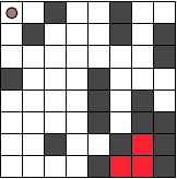
(b) #6 : unexpected

(c) #6 - mDASPAR

(d) #10: expected

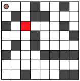
(e) #10: unexpected

(f) #10 - mDASPAR

Reachability. The expected explanations (e.g., Fig.s 4(a) and 4(d)) focus on the obstacles that surround the unreachable cells, as they prevent them from being reachable. The explanation in Fig. 4(b) puts the focus on the unreachable cells themselves, and Fig. 4(e) distinguishes a particular obstacle as a reason. When the respective abstraction mappings are given to mDASPAR, it needs to refine further to distinguish more obstacles and achieve unsatisfiability. The mark in Figure 4(e) is a possible solution to the unreachability of the cells, since removing the marked obstacle makes all the cells reachable.

In ASP, checking whether all cells are reachable is straightforward, without introducing guesses. This is also observed to be helpful for mDASPAR, as most of the resulting abstractions were similar to the gathered answers. Since in the initial abstraction, the abstract program only knows that the agent is located in the upper-left abstract region, in instance #10, mDASPAR follows a different path in refining the abstraction, and reaches the abstraction shown in Figure 4(f). Although not the same as the one given by the users, this abstraction also shows a reason for having unreachable cells.

Visitall. Most of the users pick two dead-end cells in the instances (if such occur) as an explanation for unsatisfiability. However, the explanations are given by marking these dead-end cells, instead of the obstacles surrounding them (e.g., Fig. 5(a)), which are the actual cause for them to be dead-end cells. Even with abstraction mappings that also distinguish the surrounding obstacles, the corresponding abstract program is still satisfiable. mDASPAR needs to refine further to distinguish the neighboring cells (as in Fig. 5(c)), to realize that it can only pass through one grid-cell when reaching the dead-end cells, and thus achieve unsatisfiability.

Some instances do not contain two dead-end cells, but single-cell passages to some regions. Fig. 5(d) shows an entry that distinguishes these passages, while again focusing only on the cells themselves. For these instances, the results of mDASPAR are quite different. For V${}_{\textup{KT}}$, even the abstraction mapping that extends the explanation in Fig. 5(d) by distinguishing the obstacles can not achieve unsatisfiability. This is due to guessing a set of $\mathit{move\/}$ atoms, which achieves that every cell is visited, but actually does not have a corresponding original order of movements. The abstraction does not achieve unsatisfiability for V as well. The abstract encoding is able to compute a plan that traverses over different-sized regions by avoiding the constraints due to uncertainty. Fig. 5(f) shows the best abstraction achieved for V${}_{\textup{KT}}$. It distinguishes all the cells in the one-passage-entry regions to realize that a desired action sequence can not be found.

Figure 5: Explanations for unsolvable Visitall instances

(a) #1: expected

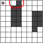
(b) #1: unexpected

(c) #1 - mDASPAR

(d) #10: expected

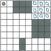
(e) #10: unexpected

(f) #10 - mDASPAR

Observations

The abstraction method can demonstrate the capability of human-like focus on certain parts of the grid to show the unsolvability reason. However, humans are also implicitly making use of their background knowledge and do not need to explicitly state the relations among the objects. Empowering the machine with such capabilities remains a challenge. The study also showed the difference in understanding the meaning of “explanation”. For some, showing the solution to get rid of unsolvability is also seen as an explanation. This difference in understanding shows that one needs to clearly specify what they want (e.g., “mark only the obstacles that cause to have unreachable cells”), which would then deviate from studying the meaning of explanation.

8 Conclusion

In this paper we introduced a novel approach for using abstraction to focus on certain aspects of problem solving in ASP. The method allows for making use of the structure in the problem for describing the abstraction, and shows an automated way of starting with an initial abstraction and achieving an abstraction with a concrete answer. We use this approach to obtain (quad-tree style) abstractions that zoom in to the reason for unsolvability of grid-cell problem instances. The user study shows that these abstractions match the intuition behind human explanations, and can be used to obtain explanations for unsolvability. Although, achieving the various levels of abstraction in human explanations is a challenge.

Related Work. The most relevant work of abstraction in AI can be seen in the planning community, which mostly focuses on abstracting the state space Sacerdoti (1974); Helmert et al. (2014); Illanes and McIlraith (2019). A syntactic approach with a hierarchical view of abstraction over the domain has not been considered. The recent work on explanations for unsolvability Sreedharan et al. (2019) focuses on projecting out irrelevant objects, similar to Saribatur and Eiter (2018).

Appendix A Computing Joint Abstract Relation Types

Abstract relations can be easily employed with abstraction mappings over several sorts in the domain as $m:D_{1}\times\dots\times D_{n}\rightarrow\hat{D}_{1}\times\dots\times\hat{D}_{n}$. If a rule has relations over the sorts, a joint abstract relation combining them must be computed.

Assuming for simplicity a uniform arity $k$, the abstract $k$-tuple relations are computed by

$$\widehat{\mathit{rel\/}}_{i}((\hat{d}_{1}^{1},...\,, \hat{d}_{1}^{n}),...\,,(\hat{d}_{k}^{1},...\,,\hat{d}_{k}^{n}))\leftarrow\mathit{rel\/}_{i}(d_{1}^{i},...\,,d_{k}^{i}),$$

$$\qquad{\textstyle\bigwedge_{j=1}^{k}}m(((d_{j}^{1},...\,,d_{j}^{n})),((\hat{d}_{j}^{1},...\,,\hat{d}_{j}^{n}))).$$

for $i=1,\ldots,n$. We compute the types of these auxiliary abstract relations, for objects $\hat{c}_{j}=(\hat{d}_{j}^{1},\dots,\hat{d}_{j}^{n}),1\leq j\leq k$.

$$\tau_{\textup{I}}^{\widehat{\mathit{rel\/}}_{i}}(\hat{c}_{1},\dots,\hat{c}_{k}) \leftarrow\widehat{\mathit{rel\/}}_{i}(\hat{c}_{1},\dots,\hat{c}_{t}),\mathit{not\/}\ \neg\widehat{\mathit{rel\/}}_{i}(\hat{c}_{1},\dots,\hat{c}_{t})$$

$$\tau_{\textup{II}}^{\widehat{\mathit{rel\/}}_{i}}(\hat{c}_{1},\dots,\hat{c}_{t}) \leftarrow\mathit{not\/}\ \widehat{\mathit{rel\/}}_{i}(\hat{c}_{1},\dots,\hat{c}_{t}),\neg\widehat{\mathit{rel\/}}_{i}(\hat{c}_{1},\dots,\hat{c}_{t})$$

$$\tau_{\textup{III}}^{\widehat{\mathit{rel\/}}_{i}}(\hat{c}_{1},\dots,\hat{c}_{t}) \leftarrow\widehat{\mathit{rel\/}}_{i}(\hat{c}_{1},\dots,\hat{c}_{t}),\neg\widehat{\mathit{rel\/}}_{i}(\hat{c}_{1},\dots,\hat{c}_{t})$$

The types of the joint abstract relation $\widehat{\mathit{rel\/}}$ over the objects $\hat{c}_{j}=(\hat{d}_{j}^{1},\dots,\hat{d}_{j}^{n}),1\leq j\leq k$ (i.e. $\tau_{\textup{I}}^{\widehat{rel}}$ and $\tau_{\textup{III}}^{\widehat{rel}}$), are then computed as below.

$$\tau_{\textup{I}}^{\widehat{rel}}(\hat{c}_{1},\dots,\hat{c}_{k}) \leftarrow\tau_{\textup{I}}^{\widehat{\mathit{rel\/}}_{1}}(\hat{c}_{1},\dots,\hat{c}_{k}),\dots,\tau_{\textup{I}}^{\widehat{\mathit{rel\/}}_{n}}(\hat{c}_{1},\dots,\hat{c}_{k})$$

$$\tau_{\textup{III}}^{\widehat{rel}}(\hat{c}_{1},\dots,\hat{c}_{k}) \leftarrow\tau_{\textup{III}}^{\widehat{\mathit{rel\/}}_{i}}(\hat{c}_{1},\dots,\hat{c}_{k}),$$

$$\quad{\textstyle\bigwedge_{j=1:j\neq i}^{n}}\mathit{not\/}\ \tau_{\textup{II}}^{\widehat{\mathit{rel\/}}_{j}}(\hat{c}_{1},\dots,\hat{c}_{k}),1\leq i\leq n.$$

Note that for the joint abstract relation $\widehat{rel}$, type $\tau_{\textup{II}}^{\widehat{rel}}$ computation is not needed, as the abstract rule construction only deals with types I and III.

References

- Brain et al. [2007] Martin Brain, Martin Gebser, Jörg Pührer, Torsten Schaub, Hans Tompits, and Stefan Woltran. Debugging ASP programs by means of ASP. In Proc. LPNMR, pp. 31–43. Springer, 2007.
- Brewka et al. [2011] Gerhard Brewka, Thomas Eiter, and Mirosław Truszczyński. Answer set programming at a glance. Comm. ACM, 54(12):92–103, 2011.
- Cabalar et al. [2014] Pedro Cabalar, Jorge Fandinno, and Michael Fink. Causal graph justifications of logic programs. TPLP, 14(4-5):603–618, 2014.
- Clarke et al. [2003] Edmund Clarke, Orna Grumberg, Somesh Jha, Yuan Lu, and Helmut Veith. Counterexample-guided abstraction refinement for symbolic model checking. J. ACM, 50(5):752–794, 2003.
- Craik [1952] Kenneth James Williams Craik. The nature of explanation, volume 445. CUP Archive, 1952.
- Erdem et al. [2016] Esra Erdem, Michael Gelfond, and Nicola Leone. Applications of answer set programming. AI Magazine, 37(3):53–68, 2016.
- Faber et al. [2004] Wolfgang Faber, Nicola Leone, and Gerald Pfeifer. Recursive aggregates in disjunctive logic programs: Semantics and complexity. In Proc. JELIA, pp. 200–212. Springer, 2004.
- Gebser et al. [2008] Martin Gebser, Jörg Pührer, Torsten Schaub, and Hans Tompits. A meta-programming technique for debugging answer-set programs. In AAAI, pp. 448–453, 2008.
- Gelfond and Lifschitz [1988] M. Gelfond and V. Lifschitz. The stable model semantics for logic programming. In ICLP/SLP, pp. 1070–1080, 1988.
- Giunchiglia and Walsh [1992] Fausto Giunchiglia and Toby Walsh. A theory of abstraction. Artificial Intelligence, 57(2-3):323–389, 1992.
- Helmert et al. [2014] Malte Helmert, Patrik Haslum, Jörg Hoffmann, and Raz Nissim. Merge-and-shrink abstraction: A method for generating lower bounds in factored state spaces. J. ACM, 61(3), 2014.
- Illanes and McIlraith [2019] León Illanes and Sheila A. McIlraith. Generalized planning via abstraction: Arbitrary numbers of objects. In AAAI, 2019.
- Johnson-Laird [1983] Philip Nicholas Johnson-Laird. Mental models: Towards a cognitive science of language, inference, and consciousness. Harvard Univ. Press, 1983.
- Kambhampati and Davis [1986] Subbarao Kambhampati and Larry Davis. Multiresolution path planning for mobile robots. IEEE Journal on Robotics and Automation, 2(3):135–145, 1986.
- Knoblock [1990] Craig A Knoblock. Learning abstraction hierarchies for problem solving. In AAAI, pp. 923–928, 1990.
- Oetsch et al. [2010] Johannes Oetsch, Jörg Pührer, and Hans Tompits. Catching the ouroboros: On debugging non-ground answer-set programs. TPLP, 10(4-6):513–529, 2010.
- Pontelli et al. [2009] Enrico Pontelli, Tran Cao Son, and Omar Elkhatib. Justifications for logic programs under answer set semantics. TPLP, 9(1):1–56, 2009.
- Sacerdoti [1974] Earl D Sacerdoti. Planning in a hierarchy of abstraction spaces. Artificial Intelligence, 5(2):115–135, 1974.
- Saitta and Zucker [2013] Lorenza Saitta and Jean-Daniel Zucker. Abstraction in artificial intelligence and complex systems, volume 456. Springer, 2013.
- Saribatur and Eiter [2018] Zeynep G. Saribatur and Thomas Eiter. Omission-based abstraction for answer set programs. In Proc. KR, pp. 42–51, 2018.
- Saribatur et al. [2019] Zeynep G. Saribatur, Peter Schüller, and Thomas Eiter. Abstraction for non-ground answer set programs. In Proc. JELIA, pp. 576–592. Springer, 2019.
- Schulz and Toni [2013] Claudia Schulz and Francesca Toni. ABA-based answer set justification. TPLP, 13(4-5-Online-Supplement), 2013.
- Sreedharan et al. [2019] Sarath Sreedharan, Siddharth Srivastava, David Smith, and Subbarao Kambhampati. Why Can’t You Do That HAL? Explaining Unsolvability of Planning Tasks. In Proc. IJCAI, 2019.