Multi-Sensor 3D Object Box Refinement for Autonomous Driving

Abstract

We propose a 3D object detection system with multi-sensor refinement in the context of autonomous driving. In our framework, the monocular camera serves as the fundamental sensor for 2D object proposal and initial 3D bounding box prediction. While the stereo cameras and LiDAR are treated as adaptive plug-in sensors to refine the 3D box localization performance. For each observed element in the raw measurement domain (e.g., pixels for stereo, 3D points for LiDAR), we model the local geometry as an instance vector representation, which indicates the 3D coordinate of each element respecting to the object frame. Using this unified geometric representation, the 3D object location can be unified refined by the stereo photometric alignment or point cloud alignment. We demonstrate superior 3D detection and localization performance compared to state-of-the-art monocular, stereo methods and competitive performance compared with the baseline LiDAR method on the KITTI object benchmark.

I INTRODUCTION

3D object detection and localization have drawn increasing attention in these years as being a core perceptual function for self-driving vehicles. Plenty of recent efforts have been made to detect 3D objects using the monocular camera [1, 2, 3, 4, 5, 6, 7], as it is low-cost and provides rich semantic information for scene understanding. However, a single camera is naturally inaccurate in 3D localization. There are also other works exploring the use of specific depth sensor such as stereo imagery [8, 9, 10, 11], which are also relatively low-cost and provide effective depth information, but have a limited sensing range; and LiDAR [12, 13, 14, 15, 16, 17, 18], which has accurate 3D localization ability, but is less informative and sensitive to reflection (e.g., rainy, car window). To achieve robust perception, modern self-driving vehicles tend to equip multiple different sensors, where the 3D information is represented in quite different ways (e.g., high-level semantic cues for the monocular image, pixel-level disparity for stereo images, sparse but geometric-aware point cloud for LiDARs). However, there is currently no explicit formulation to model the geometric relations between the object state and different kinds of raw sensor observations. As a result, naturally incorporating multiple sensors with variant characteristics brings researchers new challenges for designing a robust 3D object estimator. Although the 3D bounding box can be separately regressed in end-to-end manners, employing individual networks for each sensor leads to redundant computation, and the missing of original uncertainty information poses barriers for the future sensor fusion. In another aspect, directly learning the multi-sensor model by stacking all the sensor data into a deep neural network (DNN) might lack the interpretability and the flexibility.

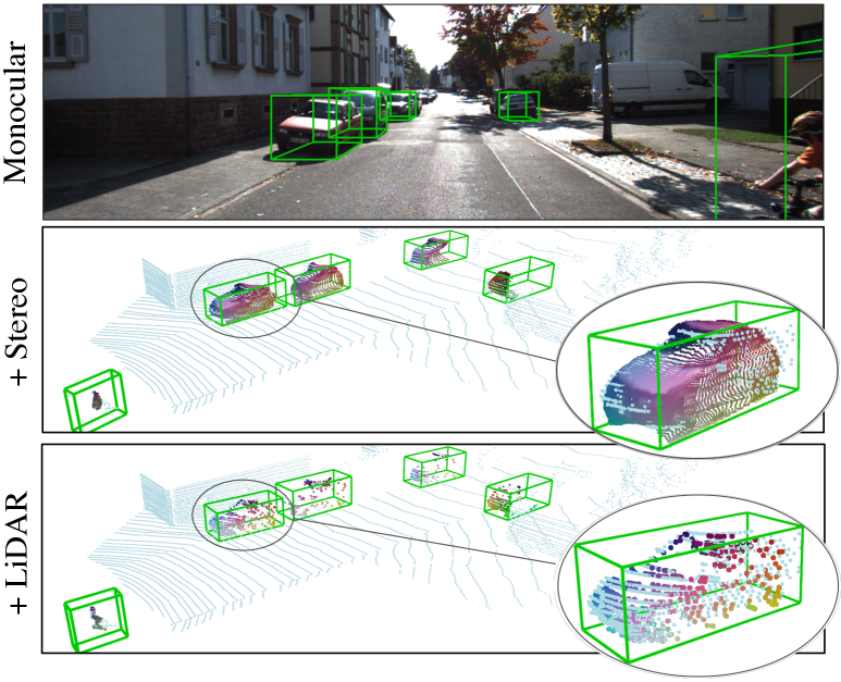
Figure 1: Example 3D object estimation results of our framework. From top to bottom: Our fundamental monocular 3D detection; Stereo refinement using the photometric alignment; LiDAR refinement using the point cloud alignment. Enlarged views show the pixel-wise or point-wise object shape which is used for geometric refinement.

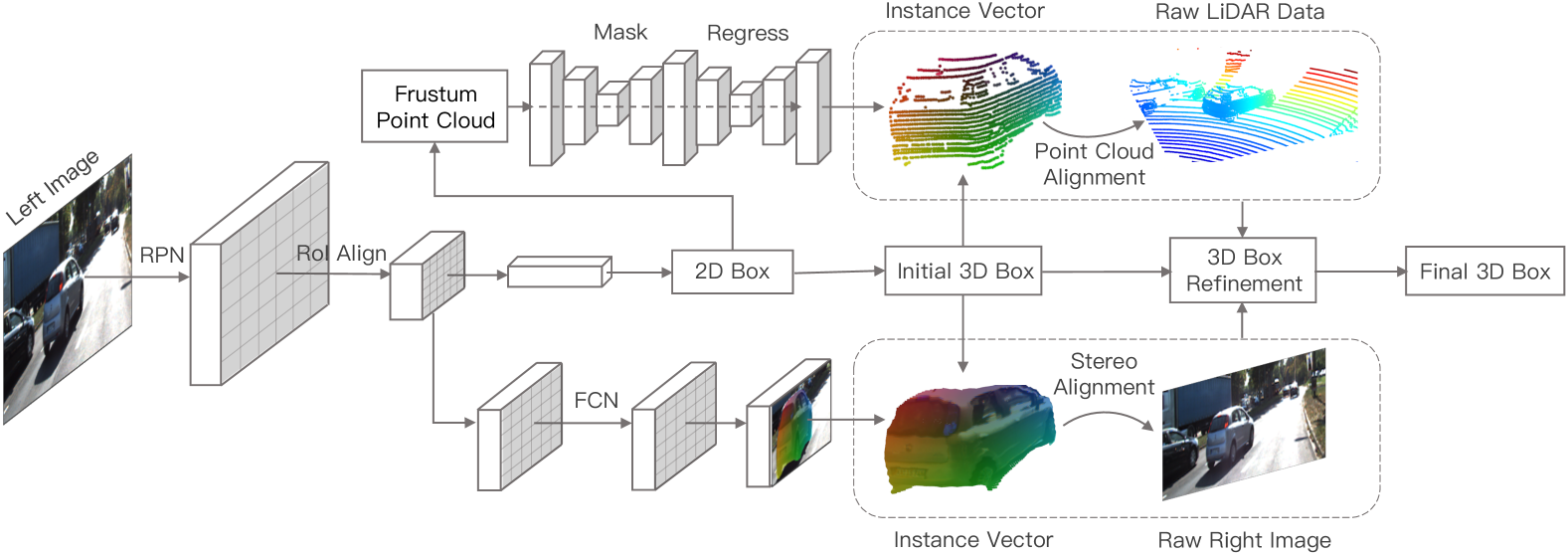
Figure 2: System architecture of our 3D object detection and refinement, where we design a light-weight monocular 3D detector (Sect. III-A) to provide 2D RoIs and initial 3D boxes. Recovering the object shape using our instance vector representation, we perform unified 3D box refinement using the stereo photometric alignment (Sect. III-B), point cloud alignment (Sect. III-C).

To this end, instead of focusing on the single modal accuracy, we aim to explicitly model the 3D geometry characterization in different sensor domain, where each sensor should be exploited their natural properties to contribute to the final 3D object estimation. Following this motivation, we design our two-stage system as shown in Fig. 2. Given a single image as the fundamental input, we extend the Faster R-CNN [19] to a light-weight monocular 3D object detector, where we predict several spatial information together with the 2D box and the object class to infer the initial 3D bounding box (Sect. III-A). To unified utilize stereo or LiDAR to refine the 3D object estimation, we model the object structural information in the image or the point cloud into a unified instance vector representation, which indicates the 3D coordinate of each raw sensor element (e.g., pixels, 3D points) respecting to the object local frame. Specifically, if stereo images are available, we employ a region-based FCN to predict the object instance vector and segmentation mask after RoIAlign [20] layer. Anchoring the masked instance vector to the initial 3D bounding box, we obtain dense object-level 3D reconstruction (bottom half of Fig. 2). The initial 3D box accuracy can then be improved by warping the shape-aware object patch from the left image to the right image and optimizing the minimum photometric error. If the point cloud is given, we adopt PointNet [21] to predict the point-wise instance vector. Similar with [13], we take the point cloud contained in the object frustum as input and perform the mask segmentation and instance vector regression sequentially. With the point-wise instance vector, each 3D point is associated with the object center to form a sparse local shape under the same representation (top half of Fig. 2). Similarly, the 3D object can be further relocalized by reprojecting the local structure to the raw LiDAR point cloud and minimizing the point-wise distance.

The instance vector has low-variance and spatial-invariant characteristics under the same object category. It is deterministically associated with the local appearance (e.g., the left-rear lamp of vehicles always appears at roughly same locations in vehicle frame) and thus considered as a suitable task for neural networks. Thanks to this unified representation, stereo cameras and the LiDAR can be treated as adaptive plug-in sensors to improve the 3D object estimation using similar energy-minimization approaches. Based on the raw sensor uncertainty, we are further able to naturally fuse multiple raw sensor measurements to jointly refine the 3D object location.

Our key contributions are summarized as 1) A simple and effective monocular 3D object detector which serves as our fundamental and backup perceptual function. 2) The first to propose a unified geometric way to utilizing the stereo images or point cloud to refine the 3D object box. 3) Demonstrate state-of-the-art 3D detection and localization performance for both monocular, stereo, and show competitive 3D performence using the LiDAR on the KITTI object benchmark.

II Related Work

II-A 3D Object Detection from Images.

Several works focus on using a single image to estimate 3D objects. They either utilize the context information such as shape prior, ground plane, and segmentation [1], or exploit geometry correspondences between 2D and 3D bounding box[2], or fit the sparse keypoint to wireframe models [4, 3]. Recently, [5, 6] propose end-to-end multi-level fusion strategies for 3D object detection, where [5] takes advantages of multidimensional input fusion, and [6] uses multi-stage feature map fusion. To complement the missed depth information in monocular images, some works exploit the stereo imagery to achieve better localization accuracy. [8, 11] take the stereo-generate depth image as input, where [8] focuses on 3D proposals generation and scoring by encoding prior and context information, and [11] processes depth into pseudo point cloud, then employs existing LiDAR-based methods [13, 15] to detect 3D objects. In another aspect, [9, 10] exploit the depth information from raw stereo images. [9] formulates spatial and temporal sparse correspondences into an object-level bundle adjustment problem. [10] takes advantage of both sparse and dense constraints in raw stereo images to achieve 3D object localization.

II-B 3D Object Detection from LiDAR.

Majority of existing 3D object detection methods rely on LiDAR to obtain accurate 3D information while representing LiDAR data in various ways. [22, 23, 24, 14, 25] quantize the raw point cloud into structured voxel grid, then use either 2D or 3D CNN to detect the 3D object. [26, 24, 27] encode the point cloud into 2D image formats by projecting raw 3D points to front view or bird’s eye view images, the 3D object detection can thereby be achieved using the regular 2D convolutional network. Benefited from the PointNet [21], [13, 28] propose to directly localize 3D objects in raw point cloud based on 2D proposals [13] or 3D proposals [28].

II-C Using Multimodal Data.

There are also some works exploiting multiple sensor fusion for 3D object detection. [12, 15] extract feature for RGB image and LiDAR-project images in separate branches then fuse the feature map by element-wise mean in the following R-CNN stage, while [16] continuously fuses the multiple sensor streams during the feature extraction stage. Instead of converting LiDAR into 2D representations, [29] processes RGB image and point cloud using ResNet [30] and PointNet [21] respectively, then employs a fusion layer to perform dense fusion. However, all the above methods realize the multimodal fusion in the network which takes specified data as input, thus are not flexible enough, i.e., one trained model weight can only be applied to a fixed sensor combination.

III 3D Object Estimation Framework

In this section, we start with our monocular 3D object detector, then describe how to extend it to the stereo and point cloud refinement. A 3D bounding box is represented with its center location $\mathbf{p}_{o}$ = $[x_{o},y_{o},z_{o}]$, dimension $\mathbf{d}$ = $[w,h,l]$, and rotation $\mathbf{R}(\theta)$ parameterized by the horizontal orientation $\theta$. As illustrated in Fig. 2, our 3D object detection framework uses the monocular image to produce 2D RoI (Region of Interest) proposals and initial 3D bounding boxes, which is described in Sect. III-A. If additional sensor inputs (e.g., stereo images, point cloud) are available, we predict element-wise mask and instance vector for each proposal, the 3D object location can then be unified refined by minimizing the stereo photometric error (Sect. III-B) or point cloud alignment error (Sect. III-C).

III-A Monocular 3D Object Detection

Our monocular 3D detector adopts a similar architecture with Faster R-CNN. We use identical region proposal network (RPN) for 2D RoIs generation. After RoI Align [20], we feed feature maps into the R-CNN head to extract high-level semantic information. Besides object classification and 2D box regression, we leverage additional fully-connected (fc) layers to predict several spatial properties to recover the 3D bounding box. Directly regressing the 3D object pose is ill-posed from the cropped image RoI due to the loss of both location and size information. We thereby employ a residual based regression to predict the 2D projection and depth of the 3D object center. Similar to 2D box prediction, we regress the normalized residual between the 2D projection of the 3D box center and the 2D RoI center:

$$\begin{aligned} \begin{array}[]{lr}\Delta u=(u_{o}-u_{\rm roi})/w_{\rm roi},\\ \Delta v=(v_{o}-v_{\rm roi})/h_{\rm roi},\end{array}\end{aligned}\rm with\begin{aligned} \begin{array}[]{lr}u_{o}=f_{x}\frac{x_{o}}{z_{o}}-u_{p},\\ v_{o}=f_{y}\frac{y_{o}}{z_{o}}-v_{p},\end{array}\end{aligned}$$ (1)

where $u_{o},v_{o}$ denote the 2D projection coordinates of the 3D object center on the image, which is determined by the object location $[x_{o},y_{o},z_{o}]$, camera focal length $f_{x},f_{y}$ and the principle point $u_{0},v_{0}$ along the $u,v$ axis respectively. $u_{\rm roi},v_{\rm roi},w_{\rm roi},h_{\rm roi}$ represent the center coordinates and the width and height of the 2D RoI. The residual of the object depth $z_{o}$ is defined as

$$\Delta z=\log(\tfrac{z_{o}}{z_{\rm roi}}),\,z_{\rm roi}=f_{y}\tfrac{h}{h_{\rm roi}},$$ (2)

where $z_{\rm roi}$ can be considered as a coarse depth which is inferred from the perspective relation between the 3D object height $h$ and 2D RoI height $h_{roi}$. We define the dimension regression term as $\Delta d=\log\frac{({d}-{p_{d}})}{\sigma_{d}},d\in(w,h,l)$, where $p_{d}$ is a dimension prior and $\sigma_{d}$ for the corresponding standard deviation. As the global orientation $\theta$ is unobservable from the local image patch [2, 31, 10], we predict the observation angle $\alpha$ which can be uniquely determined by object appearance. Inspired from [2], we employ MultiBin based orientation estimation strategy. We classify the probability that the target angle lies in k bins and regress the cosin and sine offset between the target angle and the bin’s ray direction. In summary, we have $k$ classification terms for the bin prediction, and $6+2k$ 3D box regression terms $[\Delta u,\Delta v,\Delta z,\Delta w,\Delta h,\Delta l,cos(\Delta\alpha_{i}),sin(\Delta\alpha_{i})],i\in(1,$ $\cdots,k)$ for each object category as illustrated in Fig. 3.

Figure 3: The data flow of the monocular 3D object detection. All above terms are defined in Sect. III-A.

With these predicted variables, the 3D object location can be recovered using the inverse transforming as described in Eq. 1, 2. The global orientation $\theta$ is solved by decoupling the object location and the observation angle [10]. Unlike [5] which requires depth input and [6] employs an additional network for instance depth estimation, our monocular 3D object detector is light-weight and straightforward while achieves competitive performance on the KITTI [32] benchmark. We use cross-entropy loss for object category and bin classification, smooth $L_{1}$ loss for all the regression terms. Note that we use overlapped orientation bins, so we apply the sigmoid function to the confidence outputs rather than the softmax.

III-B Stereo Photometric Alignment

The monocular image contains rich semantic information and therefore is suitable for high-level perception (e.g. foreground detection, classification). However, a single image is not able to provide accurate depth information for 3D localization. Considering this, we design our 3D object estimation framework as unified exploiting additional sensor data to refine the 3D localization.

If the stereo imagery is available, we expect to utilize it as a flexible and light-weight supplemental scheme for 3D localization enhancement instead of redeveloping a brand new stereo 3D detector. Preprocessing the stereo imagery as a dense disparity map is not only computational redundant for the only focus on the object area but also does not explicitly utilizing the object prior (e.g., object shape). Our previous work Stereo R-CNN [10] provides a heuristic for 3D bounding box refinement using raw stereo images, where the object depth is estimated according to the minimum warping cost of the object patch from the left image to the right image. However, treating the object as a regular cube unavoidably introduces shape error and limits the method to apply on general object categories (e.g., pedestrian, cyclist). To overcome this, we propose a simple approach to reconstruct the object local shape by predicting the element-wise instance vector, which represents each pixel’s normalized 3D coordinates respecting to the object instance frame, which is illustrated in Fig. 4. Similar representations are also used in [33, 34]. We normalize the physical coordinate to $[0,1]$ using the object dimension $\mathbf{d}_{o}$, which avoids the scale inconsistency issue among all pixels and multiple categories.

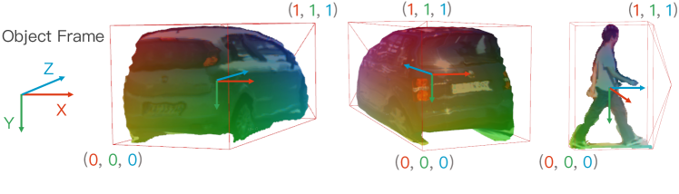
Figure 4: Illustration of the instance vector definition, where we normalize the physical coordinates to $[0,1]$ for consistency.

We adopt region-based FCN architecture proposed in [20] for element-wise instance vector prediction and mask segmentation. As illustrated in Fig. 5, after RoI Align, 14 $\times$ 14 RoI feature maps are fed to six consecutive 256-d 3 $\times$ 3 convolution layers, each followed by a ReLU layer. We use a 2 $\times$ 2 deconvolution layer with stride 2 to upsample the output scale to $28\times 28\times 4\rm c$ which contains one segmentation channel and three instance vector channels corresponding to $\rm c$ categories. Due to we predict normalized instance vector, we apply element-wise sigmoid to limit the output range between $[0,1]$.

With the masked instance vector, we are able to recover the object local shape and perform the dense stereo alignment. Let $\mathbf{u}_{i}:=[u,v]^{T}$ represents the $i^{th}$ foreground pixel in the left image, which holds the instance vector $\mathbf{v}_{i}$. We firstly recover its physical coordinate ${}^{o}\mathbf{p}_{i}$ in the object frame by scaling it with the regressed dimension $\mathbf{d}$ with element-wise multiplication $\otimes$:

$$^{o}\mathbf{p}_{i} =\mathbf{v}_{i}\otimes\mathbf{d}-\tfrac{\mathbf{d}}{2}.$$ (3)

Gathering ${}^{o}\mathbf{p}_{i}$ for all foreground pixels forms the dense object shape, the stereo alignment error $\mathbf{E}_{s}$ can then be defined as the Sum of Squared Difference (SSD) of foreground pixels over the left and right image. Let

$$\mathbf{E}_{s} :=\sum^{n}_{i=0}\left\|I_{l}(\mathbf{u}_{i})-I_{r}(\pi(^{c}\hat{\mathbf{p}}_{i}-\mathbf{b}))\right\|,$$ (4)

where we use $\pi(\mathbf{p})$ to denote projecting a 3D point $\mathbf{p}$ to the image coordinate, and $\pi^{-1}(\mathbf{u},z)$ the corresponding inverse transformation, $z$ the depth of the pixel $\mathbf{u}$. ${}^{c}\hat{\mathbf{p}}_{i}$ stands for the estimated pixel’s 3D coordinate respecting to the left camera frame, given by

$$\begin{aligned} \begin{array}[]{lr}{}^{c}\hat{\mathbf{p}}_{i}=\hat{\mathbf{p}}_{o}+\mathbf{R}(\theta)^{o}\mathbf{p}_{i},\end{array}\end{aligned}\rm with\begin{aligned} \begin{array}[]{lr}\hat{\mathbf{p}}_{o}=\pi^{-1}(\mathbf{u}_{o},\hat{z}_{o}),\end{array}\end{aligned}$$ (5)

where $\hat{\mathbf{p}}_{o}$ stands for the target 3D object location parameterized by the regressed projection $\mathbf{u}_{o}$ and the objective $\hat{z}_{o}$. Using above equations, each foreground pixel ${}^{o}\mathbf{p}_{i}$ is reprojected to the left camera frame according to the target object pose $[\hat{\mathbf{p}}_{o},\mathbf{R}(\theta)]$, further to the right camera frame according to the stereo baseline $\mathbf{b}=[b,0,0]^{T}$. As a result, we are able to rectify the 3D object depth $\hat{z}_{o}$ by minimizing the photometric error $\mathbf{E}_{o}$ of a bundle of pixel measurements.

Comparing with directly regressing the object pose in 3D space, the instance vector representation has lower variance and is associated with distinct visual cues (e.g., rear lamps, wheels). It enables us to explicitly utilize the shape prior for multi-class objects, as well as exploit geometry information in raw stereo images to achieve superior accuracy as shown in Tab.II.

Figure 5: RCNN head architecture for the pixel-wise instance vector predction and mask segmentation.

III-C Point Cloud Alignment

Based on the unified geometric relations between sensor measurements with the 3D object center (Eq. 5), we can seamlessly extend the use of instance vector representation to the raw LiDAR point cloud. To benefit from our existing monocular detection, we borrow a similar pipeline from F-PointNet [13] for the point cloud processing. As overviewed in Fig. 2, we first collect the LiDAR points inside the 2D-lifted frustum based on 2D detections. A point-wise segmentation network is then used for masking the foreground points. After that, instead of regressing object center as proposed in [13], we use PointNet [21] to predict the identical instance vector representation as defined in Fig. 4. Due to the geometric structure from the point cloud provides additional object size and orientation information, we keep the dimension and orientation regression branches in the original F-PointNet [13]. We first resample the points in the frustum to a fix number $n$, as implemented in [13]. A point-wise instance segmentation network is then employed to classify the foreground points. Using the predicted mask probability, we resample the foreground points to a fix number $m$. A light-weight T-Net [13] is then applied to predict a coarse object center, which tries to align the centroid of foreground points closer to the object center to reduce variances. We refer readers to [13] for more network details. With the aligned foreground points, we employ an instance vector regression branch which holds identical structure with the points segmentation network in parallel with the dimension and orientation regression branches. An element-wise sigmoid function is applied to the instance vector to limit its range between $[0,1]$.

Similarly with the stereo alignment, we use the point-wise instance vector $\mathbf{v}_{i}$ and the regressed dimension $\mathbf{d}$ to recover the spare local shape ${}^{o}\mathbf{p}_{i}$ using Eq. 3. The 3D object can then be relocalized by aligning the local shape to the raw point cloud. We define the point cloud alignment error $\mathbf{E}_{p}$ as the sum of Euclidean distance between reprojected foreground points with the raw point cloud. Let

$$\begin{aligned} \mathbf{E}_{p}:=\sum^{m}_{i=0}\left\|{}^{c}\mathbf{p}_{i}-{{}^{c}}\hat{\mathbf{p}}_{i}\right\|,\,\end{aligned}\rm with\begin{aligned} \begin{array}[]{lr}{}^{c}\hat{\mathbf{p}}_{i}=\hat{\mathbf{p}}_{o}+\mathbf{R}(\theta)^{o}\mathbf{p}_{i},\end{array}\end{aligned}$$ (6)

where ${}^{c}\mathbf{p}_{i}$ is the raw LiDAR point represented in the camera frame, ${{}^{c}}\hat{\mathbf{p}}_{i}$ stands for the estimated 3D point according to each point’s local coordinate ${}^{o}\mathbf{p}_{i}$ and the object pose $[\hat{\mathbf{p}}_{o},\mathbf{R}(\theta)]$. Note that we can recover the complete 3D location $\hat{\mathbf{p}}_{o}$ using the point cloud instead of only solving the center depth $\hat{z}_{o}$ in stereo alignment (refer Eq. 5). Since the orientation is regressed and treated as constant, Eq. 6 can be solved linearly. By minimizing the distance between all estimated points ${{}^{c}}\hat{\mathbf{p}}_{i}$ and the raw point cloud ${{}^{c}}{\mathbf{p}}_{i}$, we recover the accurate 3D object location which best fits the object shape, which can also be viewed in Fig. 1.

III-D Multi-Sensor Fusion

Using our 3D object estimation framework, we formulate unified spatial relations between the 3D object center and sensor elements, which are data-agnostic and operate on the raw measurement domain. We can further jointly solve the Eq. 6, 4 using raw sensor uncertainty:

$$\small\begin{split}\mathbf{p}_{o}=\operatorname*{arg\,min}_{\mathbf{p}_{o}}&\sum^{n}_{i=0}\left\|I_{l}(\mathbf{u}_{i})-I_{r}(\pi(^{c}\hat{\mathbf{p}}_{i}-\mathbf{b}))\right\|_{\sum_{s}}+\\ &\sum^{m}_{j=0}\left\|{}^{c}\mathbf{p}_{j}-{{}^{c}}\hat{\mathbf{p}}_{j}\right\|_{\sum_{p}},\end{split}\normalsize$$ (7)

where ${\scriptstyle{{\sum}_{s}}},{\scriptstyle{\sum_{p}}}$ stands for the variance of image intensity and point cloud respectively. Weighting individual error term with the raw sensor uncertainty, Eq. 7 enables us to flexibly fuse multiple sensors in a natural way to jointly refine the 3D object location $\hat{\mathbf{p}}_{o}$. Since our formulation uses unified geometric constraints from raw sensor measurements, it can be potentially applied to more general sensor configurations such as multiple stereo cameras and LiDARs.

IV Implementation Details

IV-A Loss.

Since there is no ground truth for the instance vector and mask in the KITTI object dataset [32], we calculate the label with the aid of raw LiDAR point cloud and the ground-truth 3D bounding box. We first select points which lies within the 3D bounding box as foreground samples, the point-wise instance vector $\mathbf{v}_{i}$ is then generated by

$$\mathbf{v}_{i}=({{}^{o}}\mathbf{p}_{i}+\tfrac{\mathbf{d}}{2})\oslash\mathbf{d},\,\,{{}^{o}}\mathbf{p}_{i}=\mathbf{R}(\theta)^{-1}({{}^{c}}\mathbf{p}_{i}-\mathbf{p}_{o})$$ (8)

where we transforming each LiDAR point ${{}^{c}}\mathbf{p}_{i}$ from the camera frame to the object frame ${{}^{o}}\mathbf{p}_{i}$ using the ground-truth object pose $[\mathbf{p}_{o},\mathbf{R}(\theta)]$. $\oslash$ stands for the element-wise division for normalizing the physical coordinate ${{}^{o}}\mathbf{p}_{i}$ to $[0,1]$. With the point-wise label for the foreground points from Eq. 8, we simply add an additional regression loss for the instance vector together with the other loss terms as defined in [13].

For the image, we label the sparse pixels which locate at the 2D projection of the foreground point cloud as the positive mask with the corresponding instance vector. Pixels which locate in the projection of the background points are labeled as the negative mask. We define the multi-task loss for jointly training the monocular 3D detection, the pixel-wise mask and instance vector for the image:

$$\begin{array}[]{lr}{L}=w_{rpn}L_{rpn}+w_{box}L_{box}+w_{orien}L_{orien}\\ \,\,\,\,\,\,+\,w_{loc}L_{loc}+w_{dim}L_{dim},\end{array}$$ (9)

where $L_{rpn},L_{box},L_{orien}$ denote losses for RPN, 2D detection, orientation respectively which contains both cross-entropy loss (objectness, multi-class, bin classifications) and smooth $L_{1}$ loss. $L_{loc},L_{dim}$ are smooth $L_{1}$ losses for the object location and dimension respectively. Each loss is weighted by their uncertainty as proposed in [35].

IV-B Training.

We use ResNet-101 [30] with FPN [36] as the backbone network for extracting image feature. To incorporate spatial information for 3D object inference, we concatenate pixel-wise image $u,v$ coordinates as two additional channels with the raw RGB image. For initializing the network, we simply duplicate two channels in the first convolutional layer in the imagenet-pretrained weight. We augment the data by flipping the image, where the observation angle and the instance vector are mirrored correspondingly. For point cloud, we adopt the PointNet [21] and build on top of the baseline model in [13] (denoted as v1 in the original paper).

The image and point cloud networks are trained separately since they share no feature map and gradient. We train the image network using SGD optimizer with 1 image and 512 RoIs per-batch for multi-class. The learning rate is set to 0.001 for the first 10 epochs, and reduced to 0.0001 for another 2 epochs. The PointNet is trained with exactly same hyper-parameters with the implementation in [13].

	3D Bounding Box (AP3d)									Bird’s Eye View (APbv)
	Car			Pedestrian			Cyclist			Car			Pedestrian			Cyclist
Method	Easy	Mode	Hard	Easy	Mode	Hard	Easy	Mode	Hard	Easy	Mode	Hard	Easy	Mode	Hard	Easy	Mode	Hard
Mono3D [1]	2.53	2.31	2.31	-	-	-	-	-	-	5.22	5.19	4.13	-	-	-	-	-	-
Deep3DBox [2]	5.85	4.10	3.84	-	-	-	-	-	-	9.99	7.71	5.30	-	-	-	-	-	-
Multi-Fusion [5]	10.53	5.69	5.39	-	-	-	-	-	-	22.03	13.63	11.60	-	-	-	-	-	-
MonoGRNet [6]	13.88	10.19	7.62	-	-	-	-	-	-	-	-	-	-	-	-	-	-	-
MonoPSR [7]	12.75	11.48	8.59	10.64	8.18	7.18	10.88	9.93	9.93	20.63	18.67	14.45	11.68	10.05	8.14	11.18	10.18	10.03
Ours (Mono)	16.02	13.79	12.03	10.34	9.88	9.91	13.16	11.03	11.02	20.10	16.04	15.61	10.75	10.37	10.06	13.51	11.21	11.25

TABLE I: Comparing the monocular 3D localization and detection performance with state-of-the-arts, evaluated on KITTI val set.

	3D Bounding Box (AP3d)									Bird’s Eye View (APbv)
	Car			Pedestrian			Cyclist			Car			Pedestrian			Cyclist
Method	Easy	Mode	Hard	Easy	Mode	Hard	Easy	Mode	Hard	Easy	Mode	Hard	Easy	Mode	Hard	Easy	Mode	Hard
3DOP [8]	6.55	5.07	4.10	-	-	-	-	-	-	12.63	9.49	7.59	-	-	-	-	-	-
Multi-Fusion* [5]	-	9.80	-	-	-	-	-	-	-	-	19.54	-	-	-	-	-	-	-
TLNet [37]	18.15	14.26	13.72	-	-	-	-	-	-	29.22	21.88	18.33	-	-	-	-	-	-
Stereo R-CNN [10]	54.11	36.69	31.07	-	-	-	-	-	-	68.50	48.30	41.47	-	-	-	-	-	-
Pseudo-3D [11]	56.70	37.90	34.30	23.50	19.40	15.30	28.50	19.30	18.20	74.00	54.70	47.30	32.50	27.10	23.10	35.40	23.70	22.00
Ours (Stereo)	61.96	42.03	34.57	33.65	28.60	25.47	31.60	20.58	19.12	75.13	54.19	45.12	41.62	35.95	29.74	36.30	24.02	21.85

TABLE II: Stereo 3D detection comparison using bird’s eye view AP_bv and 3D boxes AP_3d, evaluated on the KITTI val set. Multi-Fusion* [5] indicates its improved version using the stereo depth as input.

V Experiments

We evaluate our 3D object estimation framework on the KITTI object benchmark [32], which contains 7481 training samples and 7518 testing samples. Since the ground truth of test set if unavailable, we divide the training samples into train and val split following [8]. Considering the KITTI test server limits 3 submissions per month, we evaluate our monocular, stereo 3D performance on the val set as previous image-based methods do, and submit our LiDAR-based results to the test server. We compare the 3D detection (3D bounding box AP_3d) and 3D localization (bird’s eye view AP_bv) performance for car, pedestrian, cyclist with all state-of-the-are methods. We set IoU threshold to 0.7 for cars and 0.5 for pedestrians and cyclists for all experiments.

V-A Monocular Evaluation.

We first evaluate our fundamental monocular 3D detection performance. As reported in Table. I, we compare with the state-of-the-art monocular methods using Average Precision for 3D box AP_3d and bird’s eye view AP_bv on three categories, where Multi-Fusion [5] requires dense depth image as input. MonoGRNet [6] and MonoPSR [7] exploit sophisticated feature fusion strategy to encode multi-level information, while our simple-designed 3D detector is general for multiple categories and require few additional computations comparing to typical 2-stage 2D detectors. We show the overall best performance in 3D localization task and 3D detection task among car, pedestrian, and cyclist classes.

V-B Stereo Evaluation.

Benefited from our unified 3D object estimation framework, the stereo data can be seamlessly introduced into our system to refine the 3D localization accuracy. With the aid of our pixel-level stereo alignment module (Sect. III-B), the 3D detection performance can be improved significantly. The 3D bounding box AP_3d and bird’s eye view AP_3d comparison results are reported in Table. II. We list the Pseudo-3D [11] result as reported in their conference submission version, which utilizes LiDAR-based methods [15, 13] to localize the 3D object by converting the stereo-generated disparity to point cloud representation. Our previous work Stereo R-CNN [10] exploits sparse 2D bounding box and keypoints constraints to solve initial 3D box and refine object depth by dense photometric alignment. However, the box-shape approximation introduces modeling error and limits its usage on the car only. Thanks to our instance-vector based shape-aware alignment module, our method is naturally general for multiple categories objects. As Table. II reported, we show better 3D detection and localization performance compared with previous state-of-the-art stereo methods.

Note that the easier regime the object belongs, we obtain more remarkable improvements compared with other methods. This phenomenon meets our expectation since it is easier to learn a better shape for nearby objects because of more observations and denser instance vector labels. We train the car category separately for a fair comparison, all other experiments are trained jointly.

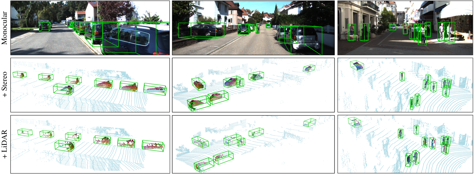
Figure 6: Qualitative examples (best view with zoom in). From top to bottom: 3D detection results using monocular, stereo images, and LiDAR point cloud, where we additionally visualize the reconstructed object shape using our instance vector representation.

V-C LiDAR Evaluation.

To demonstrate our framework is general for multiple sensors, we extend it to the use of LiDAR point cloud. We first conduct comparisons with the baseline model F-PointNet (v1) [13] which regresses the 3D object location while we solve the 3D object location by minimizing the point cloud alignment error (see Eq. 6). As shown in Table. III, when using the same 2D RoIs input, regressed orientation and dimension, our point cloud alignment method shows overall better performance on the 3D detection and localization tasks, which evidences again our instance vector based estimation is not only general for multiple sensors but also effective on the accuracy.

We further submit our result to the KITTI [32] test server. As detailed in Table. IV, we show consistent improvements comparing with the baseline F-PointNet (v1) [13]. We also list other state-of-the-art LiDAR-based methods for reference. Since our system utilizes LiDAR in the second stage only, it unavoidably underperforms the full LiDAR-based methods. Note that this letter focuses on a unified geometric 3D object estimation framework for multiple sensors and multiple categories rather than the single modal accuracy. Fully exploiting the LiDAR modality in RPN stage ([28]) or employing a more sophisticated network (e.g., PointNet++ [38]) may further improve the 3D APs while outside the scope of this work.

V-D Comparing Different Sensor Combinations.

As described Sect. III-D, our 3D estimation framework unified use different input and can perform sensor fusion in a natural way. We compare the 3D localization performance for different sensor combinations in Table. V. Same RoIs (provided in [13]) are adopted for all sensor combination to achieve clear comparison. Note that the effective range of the stereo is much smaller than the LiDAR in the KITTI setting, thus the fusion of LiDAR and stereo brings trivial improvements. We expect our uncertainty-aware estimation yields more promising gains when dealing with more general and balanced multi-sensor settings in modern self-driving cars (e.g., multiple stereos with different baseline, multiple overlapped LiDARs).

	Baseline [13]			Ours (LiDAR)
Benchmark	Easy	Mode	Hard	Easy	Mode	Hard
Car (APbv)	87.90	82.45	74.31	88.29	82.05	73.59
Pedestrian (APbv)	69.69	60.54	53.16	72.22	62.84	57.75
Cyclist (APbv)	81.00	58.61	54.55	82.48	62.68	58.30
Car (AP3d)	82.85	69.36	62.55	84.47	71.50	63.60
Pedestrian (AP3d)	65.15	55.41	48.52	67.51	57.90	50.92
Cyclist (AP3d)	76.62	54.29	50.35	78.18	57.93	54.36

TABLE III: Comparing our results with the baseline F-PointNet (v1) [13], where exactly same 2D boxes, orientation, and dimension are used for fair comparison, evaluated on the KITTI val set.

	3D Box (AP3d)			Bird’s View (APbv)
Category	Car	Ped	Cyc	Car	Ped	Cyc
VoxelNet [14]	65.11	33.69	48.36	79.26	40.74	54.76
AVOD [15]	71.88	42.81	52.18	83.79	51.05	57.48
F-PointNet (v2) [13]	70.39	44.89	56.77	84.00	50.22	61.96
PointPillar [39]	74.99	43.53	59.07	86.10	50.23	62.25
PointRCNN [28]	75.42	41.78	59.60	86.04	47.53	66.77
Baseline [13]	64.70	41.55	53.50	77.09	47.56	59.87
Ours (LiDAR)	65.33	42.87	59.40	76.65	47.78	63.72

TABLE IV: LiDAR 3D detection comparison using bird’s eye view AP_bv and 3D boxes AP_3d, reported for three categories moderate objects on the KITTI test set.

Input Data	Easy	Mode	Hard
Monocular	23.05	17.25	15.42
Monocular + Stereo	74.88	52.40	44.23
Monocular + LiDAR	88.29	82.06	73.59
Monocular + Stereo + LiDAR	88.37	82.07	73.60

TABLE V: 3D localization performance (AP_bv) of using different data, evaluated on the KITTI val set. We adopt the same 2D RoI input from [13] among all combinations for clear comparisons, the APs for the monocular and stereo thereby show slightly different performance as we reported in Table. I, II where we use our 2D detector.

V-E Qualitative Results.

We visualize some qualitative results in Fig. 6. Considering the 3D object center is invisible from raw sensor data (only the surface can be directly observed), we formulate rigorous geometric constraints between observed sensor elements with the 3D object center. Therefore, our method encourages the alignment accuracy of the nearest object surface, which is more important for obstacle avoidance in autonomous driving scenarios.

VI Conclusion and Future Work

In this latter, we aim to detect the object in the image and improve the 3D localization accuracy using multi-sensor refinement in autonomous scenarios. Using our instance vector representation, we formulate the unified spatial relations between 3D object center and raw sensor measurements. Benefited from this, we are able to exploit the individual characteristics of the different sensor while constrain the 3D object location in a unified way, which further enables us to naturally fuse multiple raw sensor data. On the 3D detection and 3D localization tasks, we outperform previous state-of-the-art monocular, stereo methods and also demonstrate competitive performance compared with the baseline LiDAR-based method.

Although our current system uses the monocular image for object proposal, our framework can seamlessly adopt 3D proposals from the point cloud to take the advantage of a high recall rate. which indicates the possible future direction of fully exploiting multiple sensors for more powerful object proposals.

References

- [1] Xiaozhi Chen, Kaustav Kundu, Ziyu Zhang, Huimin Ma, Sanja Fidler, and Raquel Urtasun. Monocular 3d object detection for autonomous driving. In European Conference on Computer Vision, 2016.
- [2] Arsalan Mousavian, Dragomir Anguelov, John Flynn, and Jana Košecká. 3d bounding box estimation using deep learning and geometry. In Computer Vision and Pattern Recognition (CVPR), 2017 IEEE Conference on, pages 5632–5640. IEEE, 2017.
- [3] Muhammad Zeeshan Zia, Michael Stark, and Konrad Schindler. Are cars just 3d boxes?-jointly estimating the 3d shape of multiple objects. In Proceedings of the IEEE Conference on Computer Vision and Pattern Recognition, pages 3678–3685, 2014.
- [4] Florian Chabot, Mohamed Chaouch, Jaonary Rabarisoa, Céline Teulière, and Thierry Chateau. Deep manta: A coarse-to-fine many-task network for joint 2d and 3d vehicle analysis from monocular image. In Proc. IEEE Conf. Comput. Vis. Pattern Recognit.(CVPR), pages 2040–2049, 2017.
- [5] Bin Xu and Zhenzhong Chen. Multi-level fusion based 3d object detection from monocular images. In IEEE CVPR, 2018.
- [6] Zengyi Qin, Jinglu Wang, and Yan Lu. Monogrnet: A geometric reasoning network for monocular 3d object localization. arXiv preprint arXiv:1811.10247, 2018.
- [7] Jason Ku, Alex D Pon, and Steven L Waslander. Monocular 3d object detection leveraging accurate proposals and shape reconstruction. In Proceedings of the IEEE Conference on Computer Vision and Pattern Recognition, pages 11867–11876, 2019.
- [8] Xiaozhi Chen, Kaustav Kundu, Yukun Zhu, Huimin Ma, Sanja Fidler, and Raquel Urtasun. 3d object proposals using stereo imagery for accurate object class detection. In TPAMI, 2017.
- [9] Peiliang Li, Tong Qin, and Shaojie Shen. Stereo vision-based semantic 3d object and ego-motion tracking for autonomous driving. In European Conference on Computer Vision, pages 664–679. Springer, 2018.
- [10] Peiliang Li, Xiaozhi Chen, and Shaojie Shen. Stereo r-cnn based 3d object detection for autonomous driving. arXiv preprint arXiv:1902.09738, 2019.
- [11] Yan Wang, Wei-Lun Chao, Divyansh Garg, Bharath Hariharan, Mark Campbell, and Kilian Weinberger. Pseudo-lidar from visual depth estimation: Bridging the gap in 3d object detection for autonomous driving. arXiv preprint arXiv:1812.07179v1, 2018.
- [12] Xiaozhi Chen, Huimin Ma, Ji Wan, Bo Li, and Tian Xia. Multi-view 3d object detection network for autonomous driving. In IEEE CVPR, volume 1, page 3, 2017.
- [13] Charles R Qi, Wei Liu, Chenxia Wu, Hao Su, and Leonidas J Guibas. Frustum pointnets for 3d object detection from rgb-d data. arXiv preprint arXiv:1711.08488, 2017.
- [14] Yin Zhou and Oncel Tuzel. Voxelnet: End-to-end learning for point cloud based 3d object detection. arXiv preprint arXiv:1711.06396, 2017.
- [15] Jason Ku, Melissa Mozifian, Jungwook Lee, Ali Harakeh, and Steven Waslander. Joint 3d proposal generation and object detection from view aggregation. arXiv preprint arXiv:1712.02294, 2017.
- [16] Ming Liang, Bin Yang, Shenlong Wang, and Raquel Urtasun. Deep continuous fusion for multi-sensor 3d object detection. In Proceedings of the IEEE Conference on Computer Vision and Pattern Recognition, pages 663–678, 2018.
- [17] Ming Liang*, Bin Yang*, Yun Chen, Rui Hu, and Raquel Urtasun. Multi-task multi-sensor fusion for 3d object detection. In CVPR, 2019.
- [18] Zhixin Wang and Kui Jia. Frustum convnet: Sliding frustums to aggregate local point-wise features for amodal 3d object detection. arXiv preprint arXiv:1903.01864, 2019.
- [19] Shaoqing Ren, Kaiming He, Ross Girshick, and Jian Sun. Faster r-cnn: Towards real-time object detection with region proposal networks. In Advances in neural information processing systems, 2015.
- [20] Kaiming He, Georgia Gkioxari, Piotr Dollár, and Ross Girshick. Mask r-cnn. In Computer Vision (ICCV), 2017 IEEE International Conference on, pages 2980–2988. IEEE, 2017.
- [21] Charles R Qi, Hao Su, Kaichun Mo, and Leonidas J Guibas. Pointnet: Deep learning on point sets for 3d classification and segmentation. Proc. Computer Vision and Pattern Recognition (CVPR), IEEE, 1(2):4, 2017.
- [22] Martin Engelcke, Dushyant Rao, Dominic Zeng Wang, Chi Hay Tong, and Ingmar Posner. Vote3deep: Fast object detection in 3d point clouds using efficient convolutional neural networks. In Robotics and Automation (ICRA), 2017 IEEE International Conference on, pages 1355–1361. IEEE, 2017.
- [23] Bo Li. 3d fully convolutional network for vehicle detection in point cloud. In Intelligent Robots and Systems (IROS), 2017 IEEE/RSJ International Conference on, pages 1513–1518. IEEE, 2017.
- [24] Wenjie Luo, Bin Yang, and Raquel Urtasun. Fast and furious: Real time end-to-end 3d detection, tracking and motion forecasting with a single convolutional net. In Proceedings of the IEEE Conference on Computer Vision and Pattern Recognition, pages 3569–3577, 2018.
- [25] Yan Yan, Yuxing Mao, and Bo Li. Second: Sparsely embedded convolutional detection. Sensors, 18(10):3337, 2018.
- [26] Bo Li, Tianlei Zhang, and Tian Xia. Vehicle detection from 3d lidar using fully convolutional network. In Robotics: Science and Systems, 2016.
- [27] Bin Yang, Wenjie Luo, and Raquel Urtasun. Pixor: Real-time 3d object detection from point clouds. In Proceedings of the IEEE Conference on Computer Vision and Pattern Recognition, pages 7652–7660, 2018.
- [28] Shaoshuai Shi, Xiaogang Wang, and Hongsheng Li. Pointrcnn: 3d object proposal generation and detection from point cloud. arXiv preprint arXiv:1812.04244, 2018.
- [29] Danfei Xu, Dragomir Anguelov, and Ashesh Jain. Pointfusion: Deep sensor fusion for 3d bounding box estimation. In Proceedings of the IEEE Conference on Computer Vision and Pattern Recognition, pages 244–253, 2018.
- [30] Kaiming He, Xiangyu Zhang, Shaoqing Ren, and Jian Sun. Deep residual learning for image recognition. In Proceedings of the IEEE conference on computer vision and pattern recognition, 2016.
- [31] Abhijit Kundu, Yin Li, and James M Rehg. 3d-rcnn: Instance-level 3d object reconstruction via render-and-compare. In Proceedings of the IEEE Conference on Computer Vision and Pattern Recognition, pages 3559–3568, 2018.
- [32] Andreas Geiger, Philip Lenz, and Raquel Urtasun. Are we ready for autonomous driving? the kitti vision benchmark suite. In Computer Vision and Pattern Recognition (CVPR), 2012 IEEE Conference on, pages 3354–3361. IEEE, 2012.
- [33] Aseem Behl, Omid Hosseini Jafari, Siva Karthik Mustikovela, Hassan Abu Alhaija, Carsten Rother, and Andreas Geiger. Bounding boxes, segmentations and object coordinates: How important is recognition for 3d scene flow estimation in autonomous driving scenarios? In Proceedings of the IEEE International Conference on Computer Vision, pages 2574–2583, 2017.
- [34] He Wang, Srinath Sridhar, Jingwei Huang, Julien Valentin, Shuran Song, and Leonidas J Guibas. Normalized object coordinate space for category-level 6d object pose and size estimation. arXiv preprint arXiv:1901.02970, 2019.
- [35] Alex Kendall, Yarin Gal, and Roberto Cipolla. Multi-task learning using uncertainty to weigh losses for scene geometry and semantics. In Proceedings of the IEEE Conference on Computer Vision and Pattern Recognition (CVPR), 2017.
- [36] Tsung-Yi Lin, Piotr Dollár, Ross B Girshick, Kaiming He, Bharath Hariharan, and Serge J Belongie. Feature pyramid networks for object detection. In CVPR, volume 1, page 4, 2017.
- [37] Zengyi Qin, Jinglu Wang, and Yan Lu. Triangulation learning network: from monocular to stereo 3d object detection. IEEE Conference on Computer Vision and Pattern Recognition (CVPR), 2019.
- [38] Charles Ruizhongtai Qi, Li Yi, Hao Su, and Leonidas J Guibas. Pointnet++: Deep hierarchical feature learning on point sets in a metric space. In Advances in Neural Information Processing Systems, pages 5099–5108, 2017.
- [39] Alex H Lang, Sourabh Vora, Holger Caesar, Lubing Zhou, Jiong Yang, and Oscar Beijbom. Pointpillars: Fast encoders for object detection from point clouds. arXiv preprint arXiv:1812.05784, 2018.